a historical analysis of natural gas demand a thesis
TRANSCRIPT

A HISTORICAL ANALYSIS OF NATURAL GAS DEMAND
A Thesis
Submitted to the Graduate Faculty
of the
North Dakota State University
of Agriculture and Applied Science
By
Nathan Richard Dalbec
In Partial Fulfillment of the Requirements
for the Degree of
MASTER OF SCIENCE
Major Department:
Agribusiness and Applied Economics
November 2014
Fargo, North Dakota

North Dakota State University
Graduate School
Title
A Historical Analysis of Natural Gas Demand
By
Nathan Richard Dalbec
The Supervisory Committee certifies that this disquisition complies with
North Dakota State University’s regulations and meets the accepted standards
for the degree of
MASTER OF SCIENCE
SUPERVISORY COMMITTEE:
Dragan Miljkovic
Chair
William Wilson
Lei Zhang
Tim Peterson
Approved:
11/21/2014 William Nganje
Date Department Chair
iii
ABSTRACT
This thesis analyzes demand in the US energy market for natural gas, oil, and coal over
the period of 1918-2013 and examines their price relationship over the period of 2007-2013.
Diagnostic tests for time series were used; Augmented Dickey-Fuller, Kwiatkowski–Phillips–
Schmidt–Shin, Johansen cointegration, Granger Causality and weak exogeneity tests. Directed
acyclic graphs were used as a complimentary test for endogeneity. Due to the varied results in
determining endogeneity, a seemingly unrelated regression model was used which assumes all
right hand side variables in the three demand equations were exogenous. A number of factors
were significant in determining demand for natural gas including its own price, lagged demand, a
number of structural break dummies, and trend, while oil indicate some substitutability with
natural gas. An error correction model was used to examine the price relationships. Natural gas
price was found not to have a significant cointegrating vector.

iv
ACKNOWLEDGMENTS
I would like to thank my advisor, Dr. Dragan Miljkovic, for his support and guidance. I
appreciate the help from my committee members, Dr. William Wilson, Dr. Lei Zhang, and Dr.
Tim Peterson for their involvement and constructive comments.
I particularly thank my lovely wife, Wenyi Dalbec, for always being there when I needed
her most. I thank my friend, Jarrett Hart, for encouraging me to get my masters. I would like to
thank all of my classmates, because without them I never would have graduated. Finally, a
special thanks to Land O’Lakes for funding this thesis.

v
TABLE OF CONTENTS
ABSTRACT ................................................................................................................................... iii
ACKNOWLEDGMENTS ............................................................................................................. iv
LIST OF TABLES ......................................................................................................................... vi
LIST OF FIGURES ...................................................................................................................... vii
INTRODUCTION .......................................................................................................................... 1
LITERATURE REVIEW ............................................................................................................... 3
LONG-RUN ECONOMIC MODEL ............................................................................................ 11
YEARLY DATA .......................................................................................................................... 12
LONG-RUN ECONOMIC PROCEDURE .................................................................................. 14
DIRECTED ACYCLIC GRAPHS ............................................................................................... 20
SEEMINGLY UNRELATED REGRESSION MODEL ............................................................. 26
SEEMINGLY UNRELATED REGRESSION RESULTS .......................................................... 28
SHORT-RUN PRICE MODEL .................................................................................................... 34
MONTHLY DATA ...................................................................................................................... 35
SHORT-RUN ECONOMETRIC PROCEDURE ......................................................................... 36
ERROR CORRECTION MODEL ............................................................................................... 42
ERROR CORRECTION RESULTS ............................................................................................ 44
CONCLUSIONS .......................................................................................................................... 48
BIBLIOGRAPHY ......................................................................................................................... 50
vi
LIST OF TABLES
Table Page
1. Augmented Dickey-Fuller Test 1918-2013 ........................................................................... 15
2. Kwiatkowski-Phillips-Schmidt-Shin Test 1918-2013 ........................................................... 16
3. Johansen Cointegration Test 1918-2013................................................................................ 17
4. Granger Causality Test 1918-2013 ........................................................................................ 18
5. Weak Exogeneity Test 1918-2013 ......................................................................................... 19
6. Correlation Matrix ................................................................................................................. 22
7. Seemingly Unrelated Regression Results .............................................................................. 29
8. Augmented Dickey-Fuller Test 2007-2013 ........................................................................... 37
9. Kwiatkowski-Phillips-Schmidt-Shin test 2007-2013 ............................................................ 37
10. Johansen Cointegration Test 2007-2013 ............................................................................... 38
11. Granger Causality Test 2007-2013 ....................................................................................... 39
12. Error Correction Results ....................................................................................................... 45
vii
LIST OF FIGURES
Figure Page
1. Consumption Graph ............................................................................................................... 11
2. PC Graph ................................................................................................................................ 23
3. GES Graph ............................................................................................................................. 24
4. Monthly Natural Gas and Oil Prices ...................................................................................... 40
5. Change in Trend and Intercept Graph .................................................................................... 41
6. Impulse Response Functions ................................................................................................. 47
1
INTRODUCTION
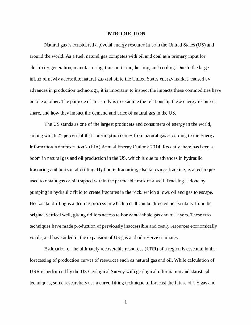
Natural gas is considered a pivotal energy resource in both the United States (US) and
around the world. As a fuel, natural gas competes with oil and coal as a primary input for
electricity generation, manufacturing, transportation, heating, and cooling. Due to the large
influx of newly accessible natural gas and oil to the United States energy market, caused by
advances in production technology, it is important to inspect the impacts these commodities have
on one another. The purpose of this study is to examine the relationship these energy resources
share, and how they impact the demand and price of natural gas in the US.
The US stands as one of the largest producers and consumers of energy in the world,
among which 27 percent of that consumption comes from natural gas according to the Energy
Information Administration’s (EIA) Annual Energy Outlook 2014. Recently there has been a
boom in natural gas and oil production in the US, which is due to advances in hydraulic
fracturing and horizontal drilling. Hydraulic fracturing, also known as fracking, is a technique
used to obtain gas or oil trapped within the permeable rock of a well. Fracking is done by
pumping in hydraulic fluid to create fractures in the rock, which allows oil and gas to escape.
Horizontal drilling is a drilling process in which a drill can be directed horizontally from the
original vertical well, giving drillers access to horizontal shale gas and oil layers. These two
techniques have made production of previously inaccessible and costly resources economically
viable, and have aided in the expansion of US gas and oil reserve estimates.
Estimation of the ultimately recoverable resources (URR) of a region is essential in the
forecasting of production curves of resources such as natural gas and oil. While calculation of
URR is performed by the US Geological Survey with geological information and statistical
techniques, some researchers use a curve-fitting technique to forecast the future of US gas and

2
oil supply. Curve-fitting methods use regression procedures to fit curves to historical trends in
production, discovery, or effort of discovery to approximate supply. These methods, however,
fail to take into account the future changes in prices, technology, or other relevant economic
factors. This shortcoming can be overcome by developing a hybrid model using econometric
techniques to estimate the relevant variables such as in the paper by Kaufmann and Cleveland
(2001).
Several papers have examined world natural gas and oil markets in order to model
production and prices. Studies of this energy market have used varying method such as linear
programing, econometrics, and curve-fitting (Hubbert, 1956; Kennedy, 1974; Krichene, 2002;
Nashawi, Malallah, and Al-Bisharah, 2010). In 2005, Dées, Karadeloglou, Kaufmann, and
Sánchez used a hybrid model that combined curve-fitting and error correction to simulate the
world oil market. This study focused primarily on the effect that OPEC countries could have on
oil prices given monopolistic or competitive behaviors. In 2002, Krichene found that there was a
significant short and long run relationship between natural gas and oil. Neither of these studies
focused strictly on the US market.
Natural gas, oil, and coal are essential to the US economy, yet no study has analyzed
these commodities together in a comprehensive way. This is also the first time directed acyclic
graphs have been used to examine the causal relationships and endogeneity issues of the US
energy market. Including the coal market in this study helps broaden the understanding of how
these energy commodities are integrated, and at what level they are substitutable with one
another. This paper focuses on the US energy market over the period of 1918-2013 using yearly
data and 2007-2013 using monthly data. For industry decision makers, this study provides
insights into the long-run relationships of natural gas demand and price.

3
LITERATURE REVIEW
The United States (US) obtains 27% of its energy from natural gas, which makes it the
second highest energy source consumed in the country (EIA Annual Energy Outlook, 2014).
During the last decade domestic natural gas and oil production have spiked due to recent
advances in hydraulic fracturing and horizontal drilling; thus the boost in production from
technological innovations led to dramatic changes in the estimation of recoverable natural gas
and oil in the US. For example, in 1995 the Bakken Shale formation in western North Dakota
was estimated to have 151 million barrels of technically recoverable oil, compared to 3.7 billion
barrels of technically recoverable oil in 2008 (Klob, 2013). These technologies have greatly
altered the energy landscape seen today in the US.
Hydraulic fracturing is a technique used to obtain gas or oil trapped within the permeable
rock of a well. The process requires hydraulic fluid which is a mixture of water, chemicals, and
proppants to be pumped down a well under high pressure to release gas and oil from the rock
bed. Proppants are usually grains of sand or similar material such as plastic pellets, steel shot,
Indian glass beads, aluminum pellets, high strength glass beads, rounded nut shells, resin-coated
sands, sintered bauxite, or fused zirconium (Klob, 2013). These materials are used to hold open
small cracks or fractures in the rock so that oil and gas can escape up the well. To date, it is
estimated that around 2.5 million fracture treatments have been performed worldwide (King &
Morehouse, 1993). Hydraulic fracturing is often used in combination with horizontal drilling.
According to a paper published by the Energy Information Agency (EIA), horizontal
drilling is a drilling process “that begins as a vertical or inclined linear bore which extends from
the surface to a subsurface location just above the target oil or gas reservoir called the "kickoff
point," then bears off on an arc to intersect the reservoir at the ‘entry point,’ and, thereafter,

4
continues at a near-horizontal attitude tangent to the arc, to substantially or entirely remain
within the reservoir until the desired bottom hole location is reached”(King & Morehouse, 1993).
In other words, horizontal drilling starts off vertically until a predetermined “kickoff point”
where the well starts to bend until it is parallel to the gas and oil deposit. Technological
breakthroughs such as downhole drilling motors and measurement equipment have made
horizontal drilling more economically feasible, which has given companies access to vast
amounts of unconventional oil and gas. Both horizontal drilling and hydraulic fracturing have
awarded producers greater access to shale gas and oil supplies.
Unconventional gas as defined by the national petroleum council in 2007 is, “natural gas
that cannot be produced at economic flow rates nor in economic volumes of natural gas unless
the well is stimulated by a large hydraulic fracture treatment, a horizontal wellbore, or by using
multilateral wellbores or some other technique to expose more of the reservoir to the wellbore.”
A major source of unconventional gas and oil is called shale gas or oil, also referred to as tight
gas or oil. These are low permeable rock formations that can be composed of sandstones,
carbonates, and shales. The EIA estimates that as of 2013 the US has roughly 223 billion barrels
of shale oil and 2,431 trillion cubic feet of technically recoverable natural gas, which makes up
26% and 27% of the world’s total shale oil and gas resources respectively (Oil Technically
Recoverable Shale, 2013).
As of 2013 the EIA estimates there are 41 countries with technically recoverable shale oil
and shale gas resources, but the US and Canada are the only two countries producing
commercially viable natural gas. There are a few reasons as to why the boom in natural gas and
oil in the US has not been replicated in other parts of the world. These include: private ownership
of mineral rights that provide an incentive for property owners to lease out their land, a large
5
number of independent competing companies and associated contractors with critical expertise,
drilling rigs, and pipeline infrastructure; access to large volumes of water for hydraulic fracturing
treatments. While there are many hurtles for countries to overcome, continued demand for
energy will drive foreign nations to consider exploiting their domestic shale gas and oil resources
(Oil Technically Recoverable Shale, 2013).
There are a variety of approaches to estimating the total supply or ultimately recoverable
resources (URR) in a particular country or region. The URR of a region can be essential in the
forecasting of production curves of resources, and can be obtained by curve-fitting historical
trends of their discovery and production. The technique of curve-fitting was established by M. K.
Hubbert (1956) in his influential article in which he forecasted the future of US oil supply by
fitting a curve to a historical production and projection data. Hubbert assumed that first,
production must decline exponentially; and second, the URR of the United States must be equal
to the area under the curve. Hubbert’s model forecasted US Oil production would peak sometime
between 1965 and 1971, and when in 1970 US production peaked many looked at Hubbert’s
method as having been correct (Strahan, 2008). Shortly after publication of his paper, several
critics produced more optimistic estimates of URR based on forecast of future drilling activity.
These discrepancies in approximating URR arise from different estimation and curve fitting
techniques.
Methods for estimating the (URR) of a region differ based on the size of the region under
study, data availability, and human resources. The methods associated with Hubbert produce
single value estimate curves fitted to historic data on production from an aggregate region, while
methods used by the US Geological Survey (USGS) yield probabilistic estimates from geological
assessments of disaggregate regions (Sorrell & Speirs, 2010). Most of the data used in methods

6
associated with Hubbert use information available in the public domain. Assessments by the US
Geological Survey extensively use geological information and complex statistical techniques
(Klett, 2005). The latter is labor intensive and usually unavailable to third parties. In other words,
Hubbert’s technique is cheaper to reproduce, faster to estimate, and easier to access since the
data used is usually publicly available.
Curve-fitting methods use regression procedures to fit curves to historical trends in
production, discovery, or effort in discovery, to estimate the URR. Each of these techniques has
a variety of strengths and weaknesses. Production over time techniques fit a curve on cumulative
production and tends to be more accurate if the production has passed its peak. The curve can
take on a variety of shapes, and one of the problems is that different functional forms often fit the
shape comparatively well but will give drastically different estimates of the URR (Ryan, 1966).
The second weakness of curve-fitting to production cycles is that they tend to have more than
one peak due to economic, technical or political changes. These changes tend to have an effect
on the shape of the curve (Laherrere, 2000). An advantage of production over time techniques is
that they rely on aggregate data rather than on information from individual fields, which tends to
be more accurate and readily available outside the US. Discovery over time techniques fit curves
to discovery trends such as proved reserves or proved and probable reserves. This method was
pioneered by Hubbert (1962) and should be more reliable because the discovery cycle is more
advanced than the production cycle. The problem with this approach is that the data is less
accessible and less reliable than production data. This process is also susceptible to reserve
growth which is when reserve estimates increase even though no new fields are discovered.
Discovery over effort techniques fit curves to an effort variable which can be measured by the
number of exploratory wells, successful exploratory wells, or length of exploratory drilling. This

7
method relies on difficult to access information, but the exploratory effort offers a better
explanatory variable than time. Finally, a major flaw shared by all of the above curve-fitting
techniques is that they require an assumption on the functional form for the production cycle.
The major flaw of curve-fitting techniques is that the assumed shape of the production or
discovery cycle is not significantly affected by the future changes in prices, technology, or other
relevant economic factors. This shortcoming is somewhat overcome by developing a hybrid
model using econometric techniques to estimate the relevant variables. In 2001, Kaufmann and
Cleveland produced a hybrid model when they included the average US production costs as an
explanatory variable, which eliminated the need to assume a functional form for the production
cycle. A weakness of this approach is that data on production costs outside the US may not be
available. The hybrid approach may be better for estimating short term supply rather than URR,
because the assumptions for estimating URR requires future values of variables (Sorrell and
Speirs 2010). While curve-fitting can be an insightful method for estimating supply, the
technological and economic unpredictability of resource discovery and reserve growth are why
this technique was not used in this study.
Some studies have attempted to forecast world oil production using different forms of the
Hubbert model but they have produced mixed results. The paper by Nashawi, Malallah, and Al-
Bisharah in 2010 used a multicycle Hubbert model to take into account technological
advancements, government regulations, economic conditions, and political events. Previous
studies have shown that a model run with one full cycle is appropriate for countries that have
production rates that do not fluctuate over time, but is not accurate in predicting production in
countries that have fluctuating rates (Ivanhou, 1995; Al-Jarri,1997; Campbell, 1998; Bartlett,
2000; Deffeyes, 2002; Szklo, Machado, Schaeffer, 2007). In their paper, peak oil production for

8
47 countries was analyzed using three procedures: correlating backdated discovery data with
production data with a shifted time lag, using known ultimate recovery, and using the method of
inflection points. The model predicted that the US, Russia, Mexico, and Canada had already
reached peak production. These predictions were solely based on conventional crude oil
production and proven reserves and did not take shale oil into account. They did not include
shale oil because it varies highly with oil prices, global economy, and available technology. Due
to this oversight, their model failed to capture the US natural gas and oil boom.
Previous approaches to modeling oil prices have used econometric techniques such as
VAR and VECM models to analyze the relation between oil prices and macroeconomic activity.
These models have attempted to demonstrate world oil markets in terms of supply and demand
equilibriums (e.g. Bacon, 1991, Al Faris, 1991). The problems that arise when modeling the
world oil markets are unique to oil, because the production from non-OPEC countries are price
takers while OPEC producing countries set their levels of production. Since OPEC determines its
level of production and installed capacity, OPECS behavior affects real oil prices (Kaufmann et
al., 2004).
To solve the problem of estimating the supply curve for OPEC countries Dées,
Karadeloglou, Kaufmann, and Sánchez in 2007 use a cartel model in which OPEC is a price
maker and a competitive model in which OPEC is a price taker. In the first model OPEC
produces only to meet demand and in the second model OPEC produces close to capacity. Oil
demand was estimated for ten global areas; US, Japan, UK, Euro area, Switzerland, other
developed economies, non-Japan Asia, transition economies, Latin America, and rest of the
world. Demand for each region was a log-linear function of real GDP, real oil prices, and a time
trend that represented technical changes in energy efficiency. Oil price was simulated using a
9
“price rule”, which measures how much OPEC must struggle to satisfy the demand for its oil and
the effect of stocks held by other nations.
The results from the study were fairly positive suggesting that it simulates real oil prices
fairly accurately. The authors simulate a price shock of 50 percent and show non-OPEC
production increase of 1.75 percent relative to the base and a 3 percent decrease in long run
demand. They also simulate a 5 percent increase in capacity which depresses the price of oil by
10 percent in the long run, which demonstrates OPEC’s reluctance to increase capacity. These
previous two cases demonstrate OPEC countries’ cooperation, but the study alternatively looked
at OPEC cooperation breaking down and production reaching 95 percent. This breakdown
caused prices to drop in the short run and demand for OPEC oil to decrease in the long run.
While this study gives valuable insight into OPEC and oil supply, it plays a small role in natural
gas markets since OPEC does not set quotas for its member states for natural gas.
In 2002 Krichene analyzed the world crude oil and natural gas output and prices during
1918-1999. He found that oil production increased steadily until 1973 when OPEC curtailed
production in an attempt to put upward pressure on prices and to prevent prices from falling out.
This shock caused non-OPEC countries to continue increasing production partially due to the
high prices. Natural gas over the same time period matched that of oil production but at a higher
rate. During the period 1973-1986 when crude oil production was stagnating, natural gas
production increased by 3.1%, signifying an increase in demand potentially due to substitution.
The study indicated that oil prices were stationary between of 1918-1973 and 1973-1999. Also
natural gas prices were non-stationary during 1918-1973, but became stationary during 1973-
1999 indicating that dynamics in the gas industry absorbed the price shocks in 1973-1986 to
bring prices back to long-term stability. A simultaneous supply and demand model was used for
10
specification and identification of elasticities. The variables used were output, prices, and real
GDP. Demand for oil in the short-run was price-inelastic and that GDP had a significant affect.
Natural gas output had a significant effect on the supply of oil, but this effect weakened after
1973, possibly due to natural gas becoming a substitute for oil given natural gas production
increased in response to oil price shocks.
Natural gas, oil, and coal are essential to the US economy, and no study has analyzed the
relationship these domestically produced commodities have with natural gas. With the recent
shale gas and oil boom exclusively in the US, it seems relevant to focus solely on the US market.
There is evidence that the fossil fuel market may be integrated since both natural gas and oil are
used in residential and commercial heating, while coal and natural gas are used heavily for
electricity generation. Since curve-fitting methods can yield inaccurate results because they do
not to take into account future changes in prices, technology, or other relevant economic factors,
they were not used in this study. There has been no study as to the impact of oil and coal on
natural gas within the US market.
11
LONG-RUN ECONOMIC MODEL
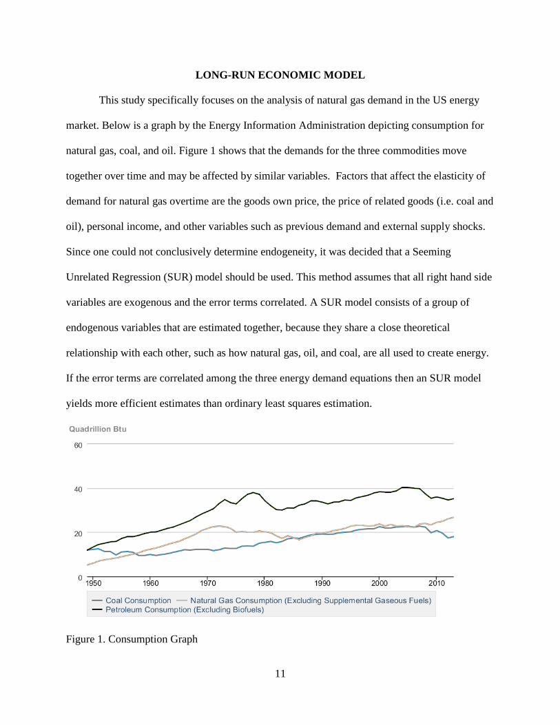
This study specifically focuses on the analysis of natural gas demand in the US energy
market. Below is a graph by the Energy Information Administration depicting consumption for
natural gas, coal, and oil. Figure 1 shows that the demands for the three commodities move
together over time and may be affected by similar variables. Factors that affect the elasticity of
demand for natural gas overtime are the goods own price, the price of related goods (i.e. coal and
oil), personal income, and other variables such as previous demand and external supply shocks.
Since one could not conclusively determine endogeneity, it was decided that a Seeming
Unrelated Regression (SUR) model should be used. This method assumes that all right hand side
variables are exogenous and the error terms correlated. A SUR model consists of a group of
endogenous variables that are estimated together, because they share a close theoretical
relationship with each other, such as how natural gas, oil, and coal, are all used to create energy.
If the error terms are correlated among the three energy demand equations then an SUR model
yields more efficient estimates than ordinary least squares estimation.
Figure 1. Consumption Graph

12
YEARLY DATA
Several variables are used in the estimation of the models: prices and consumption of
natural gas, oil, and coal, gross domestic product per capita, oil shock dummies and a time trend.
The six variables used in the study are represented as follows: natural gas price (NGP), oil price
(OILP), coal price (COALP), natural gas consumption (NGCSP), oil consumption (OILCSP),
coal consumption (COALCSP), GDP per capita (GDPPC), and oil shock dummy (OS#). The
data collected is secondary data from the Energy Information Administration, Historical
Statistics of the United States, and Bureau of Mines Minerals Yearbook. Annual data for all of
the variables was collected for the years 1918-2013, and for the US market only. Natural gas
price is based on the wellhead price, which is the price of natural gas at the wellhead including
all costs before shipment from the lease. Oil price is determined by the first purchase of crude
oil from the property. Coal price is the price of coal purchased at the mine, less freight or
shipping and insurance costs. All prices used are in nominal US dollars. Consumption for each
energy source is calculated by taking total production minus net exports. Natural gas production
is marketed production which is defined by the Energy Information Agency as, “Gross
withdrawals less gas used for repressuring, quantities vented and flared, and nonhydrocarbon
gases removed in treating or processing operations. It includes all quantities of gas used in field
and processing plant operations.” Coal production is total coal production including all types:
bituminous, subbituminous, lignite, and anthracite. Oil production is of crude oil. Quantities are
measured as follows for natural gas, oil, and coal respectively: million cubic feet, thousands of
barrels, and short tons. Prices are dollars per thousand cubic feet, dollars per barrel, and dollars
per short ton for natural gas, oil, and coal correspondingly. The oil shock dummies are used to
capture large swings in oil and natural gas prices for the following years and corresponding

13
reasons: 1920 supply shortage, 1921 gains in production from Texas, California, and Oklahoma,
1947-1948 post war demand increased due to transition to automotive transportation, 1952-1953
the end of the Korean War price controls, 1956-1957 Suez Canal crisis, 1973-1974 OPEC
embargo, 1978-1979 Iranian Revolution, 1980-1981 Iran-Iraq War, 1990-1991 First Persian Gulf
War, 1997-1998 East Asian financial crisis, 2000-2001 US recession and 911 terrorist attacks,
and 2008-2009 The Great Recession (Hamilton, 2011).

14
LONG-RUN ECONOMIC PROCEDURE
While it may seem that a relationship exists among energy commodities, it may be
difficult to accurately model it. Natural gas, oil, and coal are mined, delivered, and used in
different ways; which makes substitution difficult to show but logically plausible since they are
major energy inputs for many industries. There are five steps to test the dynamic relationship
among natural gas, oil, and coal variables which are: (1) test for unit roots to determine if the
data is stationary or follows a random walk; (2) use cointegration techniques to identify long-run
relationships; (3) test for causality among the variables using Granger causality test; (4) test for
weak exogeneity to identify variables that are determined outside the system; and (5) use a
Seemingly Unrelated Regression (SUR) model to estimate the effect and statistical significance
of exogenous variables on natural gas demand.
The Augmented Dickey-Fuller (ADF) test is used to determine if a variable has a unit
root or is stationary. A variable has a unit root, if after a shock, it does not move back to a long-
run trend. Dickey and Fuller (1979) showed that the null hypothesis of their test is that the series
has a unit root and is non-stationary. The test gives you the choice of including a constant, a
constant and a linear time trend, or none in the regression. Including the constant and trend is the
most general specification, and was the choice for this study. Also, the test allows for the
specification of the number of lagged differenced terms. A lag of one was chosen for this study
since the data is of annual prices and quantities. Based on the results of the ADF, the null
hypothesis of a unit root cannot be rejected for level data (Table 1). After the series has been
differenced once and retested, the results indicate that the null hypothesis is rejected and that the
data does not have a unit root. Thus, after first differencing all of the variables and taking the
second difference of natural gas consumption, all are integrated of order I(1) or I(2). One issue

15
with the ADF test is that it has weak power, because it only allows for the rejection of the
hypothesis that the series has a unit root rather than accepting the hypothesis that the series is
stationary.
Table 1. Augmented Dickey-Fuller Test 1918-2013
The Kwiatkowski, Phillips, Schmidt, and Shin (KPSS) test (1992) was developed to be a
complement unit root test to the ADF test. The null hypothesis of the KPSS test is that the series
is stationary which makes accepting of the null harder and gives the test a higher power. Also,
the test gives you the choice of including a constant or a constant and a linear time trend, and so
a constant and trend were chosen for the test. Based on the results of the KPSS test, the data for
all the variables, except oil price are non-stationary at the level and are stationary after first
differencing (Table 2). By using the KPSS test and ADF test one can conclude that the data does
not have a unit root and is stationary after being differenced once.
Exogenous Variables Lag Lenth ADF statistic
(levels)
ADF statistic
(first diff.)
ADF statistic
( second diff.)
NGP Constant and Trend 1 0.4834 0***
NGCSP Constant and Trend 1 0.3150 0.1875 0***
OILP Constant and Trend 1 0.9992 0***
OILCSP Constant and Trend 1 0.6874 0***
COALP Constant and Trend 1 0.8203 0.0052**
COALCSP Constant and Trend 1 0.2772 0***
* 10% significant
** 5% significant
*** 1% significant

16
Table 2. Kwiatkowski-Phillips-Schmidt-Shin Test 1918-2013
The Johansen Cointegration test is used to find the number of cointegrating vectors
among the variables (Johansen, 1991; Johansen & Juselius, 1994). Cointegration is a linear long-
run relationship between two or more variables. All of the variables must be integrated of the
same order to be cointegrated. With the results from the ADF and KPSS tests it can be concluded
that all of the variables are integrated of the order I(1). The Johansen technique uses two tests to
detect the long-run relationships; the maximal eigenvalue test and the trace test. Results from the
two tests indicate that two cointegrating vectors, at the five percent level, exist among the three
energy prices and consumptions. This means that the six variables move in response to
disequilibrium in the long run system (Table 3).
Variables Exogenous VariablesLM-Stat
(Level)
LM-Stat
(First diff.)
LM-Stat
(Second diff.)
NGP Contstant and Trend 0.233032*** 0.053528
NGCSP Contstant and Trend 0.168718* 0.107653
OILP Contstant and Trend 0.210906** 0.128380* 0.021086
OILCSP Contstant and Trend 0.192443* 0.075545
COALP Contstant and Trend .196992** 0.051226
COALCSP Contstant and Trend 0.27591*** 0.11072
* 10% significant
** 5% significant
*** 1% significant
17
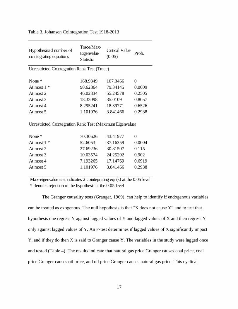
Table 3. Johansen Cointegration Test 1918-2013
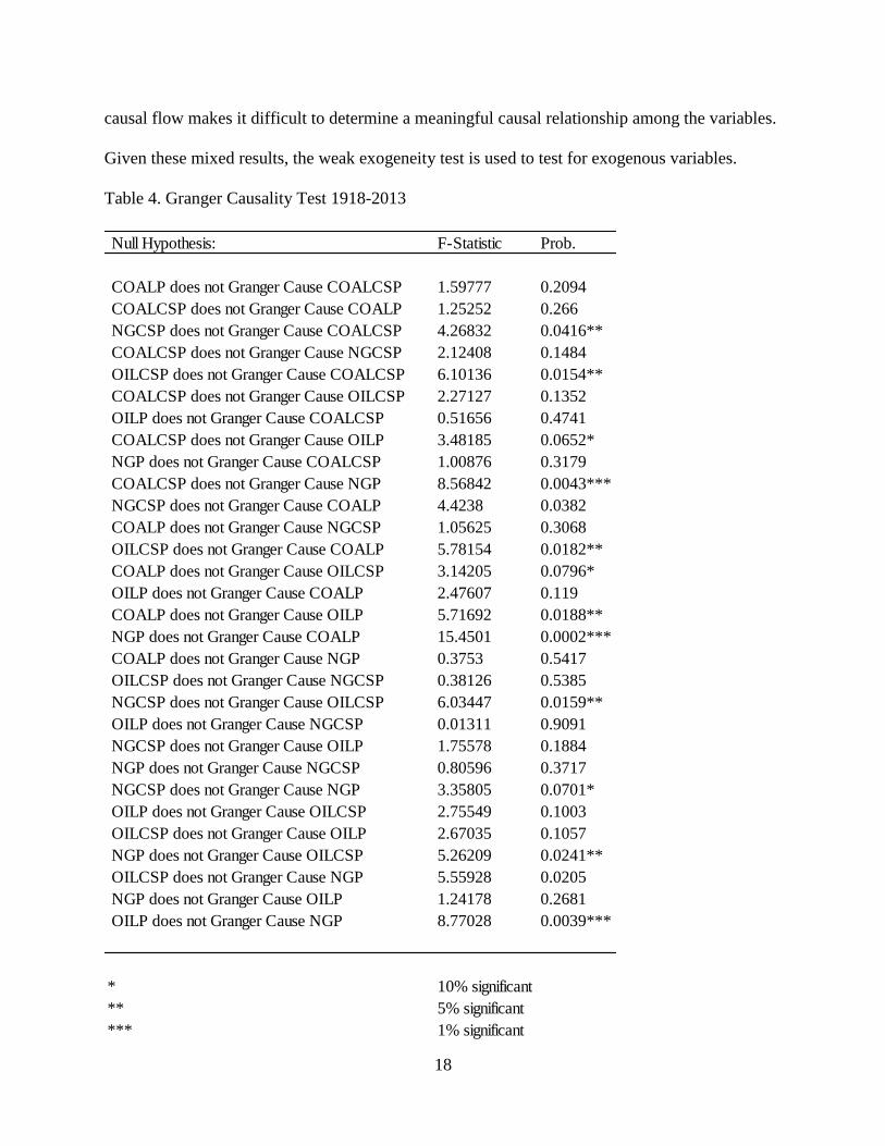
The Granger causality tests (Granger, 1969), can help to identify if endogenous variables
can be treated as exogenous. The null hypothesis is that “X does not cause Y” and to test that
hypothesis one regress Y against lagged values of Y and lagged values of X and then regress Y
only against lagged values of Y. An F-test determines if lagged values of X significantly impact
Y, and if they do then X is said to Granger cause Y. The variables in the study were lagged once
and tested (Table 4). The results indicate that natural gas price Granger causes coal price, coal
price Granger causes oil price, and oil price Granger causes natural gas price. This cyclical
Hypothesized number of
cointegrating equations
Trace/Max-
Eigenvalue
Statistic
Critical Value
(0.05)Prob.
Unrestricted Cointegration Rank Test (Trace)
None * 168.9349 107.3466 0
At most 1 * 98.62864 79.34145 0.0009
At most 2 46.02334 55.24578 0.2505
At most 3 18.33098 35.0109 0.8057
At most 4 8.295241 18.39771 0.6526
At most 5 1.101976 3.841466 0.2938
Unrestricted Cointegration Rank Test (Maximum Eigenvalue)
None * 70.30626 43.41977 0
At most 1 * 52.6053 37.16359 0.0004
At most 2 27.69236 30.81507 0.115
At most 3 10.03574 24.25202 0.902
At most 4 7.193265 17.14769 0.6919
At most 5 1.101976 3.841466 0.2938
Max-eigenvalue test indicates 2 cointegrating eqn(s) at the 0.05 level
* denotes rejection of the hypothesis at the 0.05 level
18
causal flow makes it difficult to determine a meaningful causal relationship among the variables.
Given these mixed results, the weak exogeneity test is used to test for exogenous variables.
Table 4. Granger Causality Test 1918-2013
Null Hypothesis: F-Statistic Prob.
COALP does not Granger Cause COALCSP 1.59777 0.2094
COALCSP does not Granger Cause COALP 1.25252 0.266
NGCSP does not Granger Cause COALCSP 4.26832 0.0416**
COALCSP does not Granger Cause NGCSP 2.12408 0.1484
OILCSP does not Granger Cause COALCSP 6.10136 0.0154**
COALCSP does not Granger Cause OILCSP 2.27127 0.1352
OILP does not Granger Cause COALCSP 0.51656 0.4741
COALCSP does not Granger Cause OILP 3.48185 0.0652*
NGP does not Granger Cause COALCSP 1.00876 0.3179
COALCSP does not Granger Cause NGP 8.56842 0.0043***
NGCSP does not Granger Cause COALP 4.4238 0.0382
COALP does not Granger Cause NGCSP 1.05625 0.3068
OILCSP does not Granger Cause COALP 5.78154 0.0182**
COALP does not Granger Cause OILCSP 3.14205 0.0796*
OILP does not Granger Cause COALP 2.47607 0.119
COALP does not Granger Cause OILP 5.71692 0.0188**
NGP does not Granger Cause COALP 15.4501 0.0002***
COALP does not Granger Cause NGP 0.3753 0.5417
OILCSP does not Granger Cause NGCSP 0.38126 0.5385
NGCSP does not Granger Cause OILCSP 6.03447 0.0159**
OILP does not Granger Cause NGCSP 0.01311 0.9091
NGCSP does not Granger Cause OILP 1.75578 0.1884
NGP does not Granger Cause NGCSP 0.80596 0.3717
NGCSP does not Granger Cause NGP 3.35805 0.0701*
OILP does not Granger Cause OILCSP 2.75549 0.1003
OILCSP does not Granger Cause OILP 2.67035 0.1057
NGP does not Granger Cause OILCSP 5.26209 0.0241**
OILCSP does not Granger Cause NGP 5.55928 0.0205
NGP does not Granger Cause OILP 1.24178 0.2681
OILP does not Granger Cause NGP 8.77028 0.0039***
* 10% significant
** 5% significant
*** 1% significant

19
According to Johansen and Juselius (1994), restriction to the Cointegration vector can be
used to detect structural relationships. Weak exogeneity of a variable can be tested to identify the
effect it may have on the others in the long-run. Since there are two cointegrating vectors, the
null hypothesis of weak exogeneity is accepted if the estimated coefficients of each variable in
the two cointegrating vectors are both equal to zero. Based on the results, the null hypothesis of
weak exogeneity is rejected for natural gas price, coal price, and coal consumption, while one
can accept the null for oil price, oil consumption, and natural gas consumption (Table 5). Hence,
in the long-run, the results indicate that oil price, oil consumption, and natural gas consumption
drive the price of natural gas, coal, and coal consumption.
The weak exogeneity results are inconsistent with the Granger causality test, and fail to
show any clear signs of causation or endogeneity. To further test and confirm the causal structure
of this market, directed acyclic graphs (DAGs) were used to show causality and exogeneity.
Given that DAGs examine contemporaneous causal relationships rather than lagged relationships
among variables, they complement the Granger causality and weak exogeneity tests.
Table 5. Weak Exogeneity Test 1918-2013
NGP NGCSP
Cointegration Restrictions: A(3,1) = 0 A(6,1) = 0 A(4,1) = 0 A(5,1) = 0 A(1,1) = 0 A(2,1) = 0
A(3,2) = 0 A(6,2) = 0 A(4,2) = 0 A(5,2) = 0 A(1,2) = 0 A(2,2) = 0
Chi-square(2) 21.22642 1.372653 3.885742 1.288699 27.78548 5.33744
Probability 0.000025 0.503422 0.143292 0.525004 0.000001 0.069341
Variables OILP OILCSP COALP COALCSP

20
DIRECTED ACYCLIC GRAPHS
Directed acyclic graphs (DAGs) are visual representations of defined causal flows
between and among a set of variables. These graphs were developed in the fields of artificial
intelligence and computer science. DAGs use algorithms programed into a computer to illustrate
causal relations from observational data (Lauritzen and Richardson, 2002). The recent
applications of DAGs in applied economics have been used by Roh and Bessler (1999), Bessler
and Yang (2003), and Li, Woodard, and Leatham (2013). Mathematically, these graphs represent
conditional independence as shown by the recursive product decomposition:
( ) ∏ ( ) (Eq.1)
where pr is the probability of the variables( ), and represents the realization of
some subset of the variables that cause in order ( ). The character ∏ is the
product operator. Due to the contributions by Pearl (1986, 1995), the independencies and direct
causes implied by the above equation can be translated graphically using the d-separation
criteria. Spirtes et al. (2000) was able to incorporate Pearl’s work on d-separation into algorithms
that build DAGs. D-separation can be explained using a three variable set X, Y, and Z.
Variables are said to be d-separated if the flow of information between them is blocked. This
can occur in two ways: (1) when one variable is the cause for two variables, say Y in the graph
, or when Y is the passthough variable in graph ; (2) if Y is the common
effect of two variables such as in the graph .
There are two algorithms that this study will focus on, PC and GES. The PC algorithm
starts with a complete undirected graph. An undirected graph has every variable connected to
each other with a line called an edge, which does not include any directional arrows. Then the
21
edges between the variables are removed systematically based on vanishing zero-order
correlation or higher-order correlation at a predetermined significance level of the normal
distribution. The remaining edges are directed using the theories of sepsets. There are two
problems with the PC algorithm when examining sample sizes of 100 or less; edge exclusion or
inclusion and edge direction. This can be overcome by adjusting the significance level higher to
between 20% and 30% (Spirtes et al.,p 116).
The GES algorithm uses a different approach to creating DAGs that uses Bayesian
posterior scores to search over alternative DAGs. The algorithm’s first step is to begin with a
DAG that has no edges connecting any of the variables. Then edges are added and/or directions
reversed in a search across all possible DAGs to improve the Bayesian posterior score. Once a
local maximum of the Bayesian score is found, which occurs when no edges or directions can be
added, then edges are deleted or directions reversed as long as such actions improve the Bayesian
posterior score (Chickering, 2002).
The two algorithms provide alternative approaches to analyzing empirical data. The PC
algorithm starts with completed unidirectional graph and removes edges and adds directions
based on zero correlation and partial correlations, while the GES algorithm begins with an
independent graph and adds edges and directions based on the Bayesian posterior score. These
methods were chosen for this study to give insight in to the causal relationships shared by the
variables of interest, since the results from the Granger causality test and weak exogeneity tests
were inconsistent. The PC and the GES algorithms are embedded in the software TETRAD IV,
which was used in this study.
The Directed Acyclic Graphs (DAGs) were used as an alternative way to examine causal
relationships between the variables selected for this study. The variables used for the graphs are

22
the three commodities, natural gas, oil, coal, and their prices and corresponding demands. GDP
per capita was added and is constrained in both models so that it cannot be caused by any of the
other variables, since it is assumed to be exogenous. The correlation matrix for the graphs is
displayed below.
Table 6. Correlation Matrix
This matrix is the starting point for the PC algorithm which begins with a completed
unidirectional graph and removes lines and includes directions based on zero correlation and
partial correlations. The correlation matrix shows that all of the variables are significantly
correlated with at least one other variable so it can be expected that direct and indirect casual
flows exist among the variables.
Correlation
Probability COALP COALCSP GDPPC NGP NGCSP OILCSP OILP
COALP 1.000000
-----
COALCSP 0.856419 1.000000
0.0000 -----
GDPPC 0.916216 0.943950 1.000000
0.0000 0.0000 -----
NGP 0.837725 0.860428 0.911109 1.000000
0.0000 0.0000 0.0000 -----
NGCSP 0.763920 0.701163 0.749640 0.631983 1.000000
0.0000 0.0000 0.0000 0.0000 -----
OILCSP 0.810193 0.763370 0.794607 0.693943 0.977171 1.000000
0.0000 0.0000 0.0000 0.0000 0.0000 -----
OILP 0.900357 0.741372 0.864519 0.849926 0.585654 0.608362 1.000000
0.0000 0.0000 0.0000 0.0000 0.0000 0.0000 -----

23
The DAGs for the PC algorithm are found in figure 2 at the 10 percent and 20 percent
significance levels. At the both significant levels the graph indicates that there is a causal flow
from GDP per capita to natural gas price, natural gas consumption, coal price, and coal
consumption. There are directed lines from natural gas price to oil price and natural gas
consumption to oil consumption. Finally, coal price has two causal flows from both GDP per
capita and oil consumption.
Figure 2. PC Graph
The DAG for the GES algorithm is displayed in figure 3. Recall that the GES algorithm
begins with a graph of independence among all of the variables and no choice of significance
levels. As one can see from the graph, the same exogeneity issues from the Granger causality test
and the weak exogeneity test are still present. Coal consumption is the only variable that is
completely endogenous in the system, affected by oil price, natural gas consumption, natural gas

24
price, and coal price; while the graph shows that oil price is weakly exogenous being caused by
oil consumption, natural gas consumption, natural gas price, and coal price. As seen in the PC
graph there is a causal flow from GDP per capita to natural gas price and then to oil price. The
direction of the arrow from natural gas consumption to oil consumption in the PC model is
reversed in the GES model, which indicates that demand for oil drives demand for natural gas.
Also, there is again a connection between oil demand and coal price, but it is undirected which
means the algorithm could not determine the causal flow given the available information. This
indicates that there is a variables missing between coal price and coal consumption.
Figure 3. GES Graph
To determine the appropriateness of the DAGs generated by the PC and GES algorithms,
a chi-square test is performed. The null hypothesis of the test is that, “the population covariance
matrix over all the measured variables is equal to the estimated covariance matrix over all the

25
measured variables written as a function of the free model parameters.” (TETRAD IV User’s
Manual). If one fails to reject then the causal structure estimated from the covariance matrix is
expected to be valid. Both of the PC graphs had a p-value of 0, while the GES graph had a p-
value of 0.3783, indicating that the GES graph fits the data better.
26
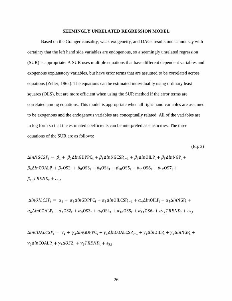
SEEMINGLY UNRELATED REGRESSION MODEL
Based on the Granger causality, weak exogeneity, and DAGs results one cannot say with
certainty that the left hand side variables are endogenous, so a seemingly unrelated regression
(SUR) is appropriate. A SUR uses multiple equations that have different dependent variables and
exogenous explanatory variables, but have error terms that are assumed to be correlated across
equations (Zeller, 1962). The equations can be estimated individuality using ordinary least
squares (OLS), but are more efficient when using the SUR method if the error terms are
correlated among equations. This model is appropriate when all right-hand variables are assumed
to be exogenous and the endogenous variables are conceptually related. All of the variables are
in log form so that the estimated coefficients can be interpreted as elasticities. The three
equations of the SUR are as follows:
(Eq. 2)

27
The oil price shock dummy variables included in the model were added based on the
paper by Hamilton (2011). The oil shocks identified by Hamilton were mostly external shocks to
the supply of oil to the United States, and were then tested using Chow’s breakpoint test to see if
these shocks caused a structural change in the demand for natural gas, oil and coal. The Chow
test splits the equation at the breakpoint into two subsamples and then compares the fit of each
subsample to the original equation (Chow, 1960). The test compares the sum of squared residuals
from the fitted single equation to the entire sample’s sum of squared residuals from each
subsample’s equations. A significant difference in the estimated equations indicates that a
structural change in the relationship has occurred. One drawback of the Chow test is that it
requires that each subsample have at least as many observations as the number of coefficients in
the estimated equation. This causes problems when trying to estimate structural changes near the
beginning or end of a data set.
28
SEEMINGLY UNRELATED REGRESSION RESULTS
The SUR model can be seen in table 7 and is estimated in logarithms, thus the results are
in the form of elasticities. This model is a simultaneous equation model representing three
endogenous demand variables; natural gas consumption, oil consumption, and coal consumption.
The equation of primary interest is natural gas consumption which represents the quantity
demand and supply in equilibrium. Note that the R2 for the natural gas equation is .568 which
means that over 56 percent of the variation in natural gas consumption is explained by the model.
Also, the intercept is positive and significant. The Durbin H statistic was calculated to test for
serial correlation due to the presence of lagged dependent variables. The results indicate that we
can accept the null hypothesis of no serial correlation for the oil and coal equations and reject the
null for the natural gas equation at the 5 percent level. By assuming the error terms are correlated
across all endogenous variables, the SUR model improves the efficiency of the natural gas
equation by including the oil and coal equations.

29
Table 7. Seemingly Unrelated Regression Results
NGCSP OILCSP COALCSP
0.056936*** .048354*** -0.03639**
[5.049704] [3.543052] [-2.20534]
0.525871*** 0.304855*** 1.045606***
[7.169425] [3.301611] [8.526436]
0.163838**
[2.224516]
0.061023
[.727294]
-0.27408***
[-3.93528]
-0.07791** 0.034416 -0.03249
[-2.38476] [0.831201] [-0.61518]
0.067098** -0.07472** 0.008534
[2.448328] [-2.13154] [0.186359]
-0.07741 0.132325* -0.01145
[-1.3126] [1.785134] [-0.13448]
0.029431 0.027635 0.022112
[0.904779] [.662965] [0.403017]
0.009311 0.018916
[0.298259] [.501794]
0.01508 -0.024624
[.490475] [-0.6549]
-0.06231 -0.07665*
[-0.164196] [-1.65232]
-0.048759** -0.06743**
[-2.0984] [-2.37896]
0.010937
[.372423]
-0.00091*** -0.00073*** -0.0000227
[-4.90222] [-3.15643] [-0.9387]
R-squared 0.56864 0.302731 0.511912
Adj. R-squared 0.503936 0.208041 0.471717
Durbin H Statistic 1.701 1.163 -0.403
OS5
OS6
OS7
TREND
OS2
OS4
COALCSP(-1)
NGP
OILP
COALP
OS3
OILCSP(-1)
Independent Variables Dependent Variables
Intercept
GDPPC
NGCSP(-1)

30
The first variable of interest is Gross Domestic Product per capita (GDPPC), which is
significant and positive. Since the dependent and independent variables are in logarithmic form,
the coefficients of the variables can be interpreted as a percentages change in the independent
variables causes a percentage change in the dependent variable. Thus, the coefficient for the
GDPPC can be interpreted as a 10 increase in GDPPC causes a 5.258 percent increase in
quantity demanded. As stated earlier, the value of the coefficient for GDPPC can be interpreted
as income elasticity of demand, and is defined mathematically in the following equation:
(Eq. 3)
Income elasticity of demand can be defined as a percentage change in quantity demanded given a
percentage change in income. Since the coefficient of GDPPC is between 0 and 1 it has low-
income elasticity, which means that an increase in income increases quantity demanded but by a
proportionately lower amount. Goods that increase in demand when income increases are
considered normal goods; while goods that increase in demand when income increases, but at a
proportionally less amount, are considered necessary goods. Necessary goods are goods that are
needed to survive and are not demanded less when income decreases, for example food, water,
and energy. This is observed in Engel’s law, when the percentage of income spent on food
decreases as income increases. Since, natural gas is used in heating and electricity generation one
can conclude that it is a necessity that is not purchased proportionately more when income rises.
The next variable that is significant and positive is lagged natural gas consumption
(NGCSP). The coefficient can be interpreted as a 10 percent increase in the previous year’s
natural gas demand causes a 1.638 percent increase in current demand. This increase in current
demand may be due to habits formed the previous year, affecting the current year’s demand.

31
Similarly, the previous increase in demand may be reinforcing the need for the commodity to be
consumed.
The next set of variables, natural gas, oil, and coal price represent price and cross-price
elasticities of demand. Price elasticity of demand measures the percentage change in quantity
demanded given a percentage change in a good’s own price, and cross-price elasticity of demand
measures the percentage change in the quantity demanded of a good given a percentage change
in the price of a different good. The mathematical formulas for price elasticity (Eq. 4) and cross-
price elasticity (Eq. 5) are as follows:
(Eq. 4)
(Eq. 5)
The price elasticity is almost always negative, which conforms to the law of demand, except in
the case of Giffen goods. Cross-price elasticities can be either positive or negative depending on
whether the goods are substitutes or complements.
The coefficient of natural gas price can be interpreted as an own price elasticity that is
negative and statistically significant. This represents the expected downward sloping demand
curve where price is on the Y-axis and quantity is on the X-axis. Since, the variable is own price
elasticity it can be interpreted as a 10 percent increase in the price of natural gas causes a .7791
percent decrease in quantity demanded. The percentage change in quantity demanded of natural
gas is proportionally less than the percentage change to the price, which indicates that natural gas

32
is relatively inelastic when it comes to its own price. Natural gas being inelastic relative to its
own price suggests that consumers are not very sensitive to changes in the price of natural gas.
The oil price variable represents the cross-price elasticity of demand between oil and
natural gas. The coefficient is significant and positive which suggests that natural gas and oil are
substitutes. If natural gas and oil are substitutes, then a 10 percent increase in the price of oil
decreases quantity demanded for oil, which causes quantity of demand for natural gas to increase
by .6709 percent and shifts the demand curve for natural gas to the right. These results suggest
that these commodities are substitutable producer goods that are both used in heating and
electricity, but given the magnitude of the value their substitutability is minimal or potentially
nonexistent.
The last cross-price elasticity to interpret is coal price, which is insignificant and
negative. This means that a 10 percent increase in the price of coal decreases quantity demanded
for coal, which causes demand for natural gas to decrease by .7741 percent and shifts the demand
curve for natural gas to the left. Coal and natural gas are complementary goods given the
negative sign of the coefficient, but these results are of low magnitude and are insignificant.
The last two significant variables are the oil shock dummy (OS6) which covered the
1978-79 Iranian revolution and the 1980-81 Iran-Iraq war, and the time trend. To interpret the
trend and the oil shock coefficients, some calculations must be made to increase the accuracy,
because as the change in the log (NGCSP) becomes disproportionately larger as the trend
increases. A more accurate estimation is obtained by using the following formula:
( ) ) (Eq. 6)

33
Using the above formula, natural gas consumption decreases by .95 percent after 10 years. This
decrease in consumption over time may be due to increased energy efficiency or more energy
commodities entering the market such as nuclear power, bio fuels, solar, and wind energies.
The Iranian oil shock represents a negative and significant 4.76 percent decrease in the
quantity demand for natural gas. This corresponds to the large increase in the price of natural gas
during this period and is explained by the own price elasticity of natural gas being negative.
Thus, the increase in price during the Iranian oil crises explains the decrease in quantity
demanded of natural gas in the United States over that time.
34
SHORT-RUN PRICE MODEL
The second portion of this thesis focuses on the price relationship shared among natural
gas, oil, and coal. The data covers the period 2007:1-2013:12 and encompasses the global
financial crises and the production boom from shale gas and oil. Examining the price relationship
natural gas shares with oil and coal is important to our understanding of how these prices behave
in the short-run. An error correction model was used in this section to take advantage of the lag
structure of the price variables and to examine the long and short-run dynamics of fossil fuel
prices.

35
MONTHLY DATA
The variables used in the model are oil price, natural gas price, coal price, an overall time
trend, net energy exports (EEXP), GDP per capita (GDPPC), US dollar index (USD), Dow Jones
Industrial Average (DOW), natural gas from fracking (FRACK), and an intercept (C2) and trend
change (T2) dummies. Monthly data for all of the variables was collected for the period between
January 2007 and December 2013 with a total of 84 observations. Energy prices and net energy
exports were obtained from the Energy Information Administration website (EIA.gov). GDP per
capita was obtained from ycharts.com and the Bureau of Economic Analysis. The US dollar
index was also found at ycharts.com. The monthly average for the Dow Jones Industrial average
was taken from yahoo finance. Natural gas from fracking was taken from the Energy Information
Agency website. Natural gas price is based on the Industrial price which is, “The price of natural
gas used for heat, power, or chemical feedstock by manufacturing establishments or those
engaged in mining or other mineral extraction as well as consumers in agriculture, forestry,
fisheries and construction.” (EIA.com). Oil price is determined by the first purchase of crude oil
from the original property. Coal price is the price of Sandy Barge 12000btu bituminous coal, less
freight or shipping and insurance costs. All prices used are in nominal US dollars. Prices are
dollars per thousand cubic feet, dollars per barrel, and dollars per short ton for natural gas, oil,
and coal correspondingly. Finally, all of the variables were logged except the net energy exports

36
SHORT-RUN ECONOMETRIC PROCEDURE
While it may seem that a relationship exists among energy commodities, it may be
difficult to accurately model them. Natural gas, oil, and coal are mined, delivered and used in
different ways, which makes substitution difficult to show but logically plausible since there is
some overlap. There are five steps to test the dynamic relationship among natural gas, oil, and
coal. These variables are: (1) test for unit roots to determine if the data is stationary or follows a
random walk; (2) use cointegration techniques to identify long-run relationships; (3) test for
weak exogeneity to find variables that are determined outside the system; (4) test for causality
among the variables using Granger causality test; and (5) use the Perron method to test for a
structural break in the series.
The Augmented Dickey-Fuller (ADF) test is used to determine if a variable has a unit
root or is stationary. Including the constant and trend is the most general specification, and was
the choice for this study. Also, the test allows for the specification of the number of lagged
differenced terms. A lag of one was chosen for this study based on the lowest values of the
Schwarz Information Criterion (SIC). Based on the results of the ADF test on each of the
variables, the null hypothesis of a unit root cannot be rejected for level data (Table 8). Once the
series is differenced once and retested, the results indicate that the null hypothesis is rejected and
that the data does not have a unit root. Thus, after first differencing, all of the variables are
integrated of order I(1).

37
Table 8. Augmented Dickey-Fuller Test 2007-2013
The Kwiatkowski, Phillips, Schmidt, and Shin (KPSS) test (1992) was developed to be a
complement unit root test to the ADF test. The null hypothesis of the KPSS test is that the series
is stationary. Also, the test gives you the choice of including a constant or a constant and a linear
time trend. As stated previously, a constant and trend were chosen for the test. Based on the
results of the KPSS test, the null hypothesis is not rejected for all the variables after first
differencing (Table 9). By using the KPSS test and ADF test it can be concluded that the data
does not have a unit root and is stationary after being differenced once.
Table 9. Kwiatkowski-Phillips-Schmidt-Shin test 2007-2013
The Johansen Cointegration test is used to find the number of cointegrating vectors
among the variables (Johansen, 1991; Johansen & Juselius, 1994). Cointegration is a linear long-
run relationship between two or more variables. All of the variables must be integrated of the
Exogenous Variables Lag Lenth ADF statistic
(levels)
ADF statistic
(first diff.)
NGP Constant and Trend 1 0.1494 0***
OILP Constant and Trend 1 0.0296** 0***
COALP Constant and Trend 4 0.0072*** 0.0048***
* 10% significant
** 5% significant
*** 1% significant
Variables Exogenous VariablesLM-Stat
(Level)
LM-Stat
(First diff.)
NGP Contstant and Trend 0.290431*** 0.044676
OILP Contstant and Trend 0.209999*** 0.027813
COALP Contstant and Trend 0.136533* 0.030205
* 10% significant
** 5% significant
*** 1% significant
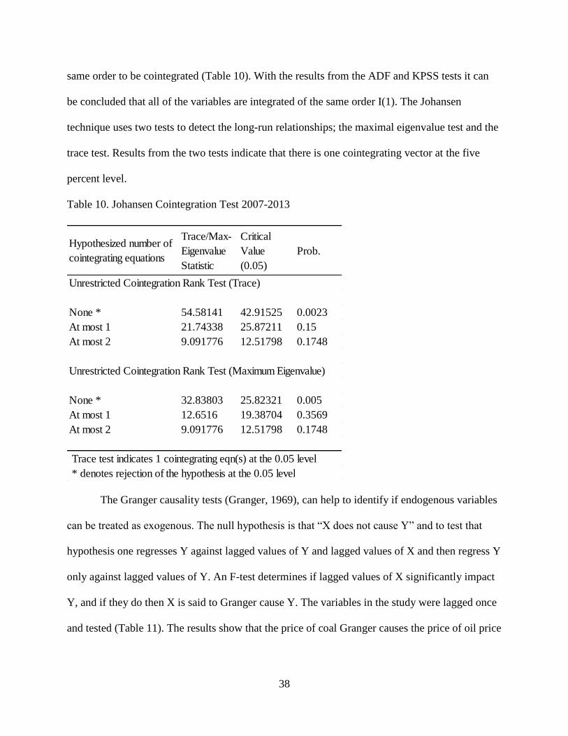
38
same order to be cointegrated (Table 10). With the results from the ADF and KPSS tests it can
be concluded that all of the variables are integrated of the same order I(1). The Johansen
technique uses two tests to detect the long-run relationships; the maximal eigenvalue test and the
trace test. Results from the two tests indicate that there is one cointegrating vector at the five
percent level.
Table 10. Johansen Cointegration Test 2007-2013
The Granger causality tests (Granger, 1969), can help to identify if endogenous variables
can be treated as exogenous. The null hypothesis is that “X does not cause Y” and to test that
hypothesis one regresses Y against lagged values of Y and lagged values of X and then regress Y
only against lagged values of Y. An F-test determines if lagged values of X significantly impact
Y, and if they do then X is said to Granger cause Y. The variables in the study were lagged once
and tested (Table 11). The results show that the price of coal Granger causes the price of oil price
Hypothesized number of
cointegrating equations
Trace/Max-
Eigenvalue
Statistic
Critical
Value
(0.05)
Prob.
Unrestricted Cointegration Rank Test (Trace)
None * 54.58141 42.91525 0.0023
At most 1 21.74338 25.87211 0.15
At most 2 9.091776 12.51798 0.1748
Unrestricted Cointegration Rank Test (Maximum Eigenvalue)
None * 32.83803 25.82321 0.005
At most 1 12.6516 19.38704 0.3569
At most 2 9.091776 12.51798 0.1748
Trace test indicates 1 cointegrating eqn(s) at the 0.05 level
* denotes rejection of the hypothesis at the 0.05 level

39
and oil price Granger causes coal price. Given these results, coal price can be treated as
endogenous.
Table 11. Granger Causality Test 2007-2013
The Perron method tests whether a time series has a single structural break characterized
by a change in intercept, trend, or both trend and intercept (Perron, 1989). The null hypothesis is
that the series has a unit root and possibly nonzero drift. This is generalized into three different
models: one that allows an exogenous change in the intercept, one that allows for an exogenous
change in the rate of growth, and one that allows for both a change in the intercept and rate of
growth. The third situation was chosen after running all three models, because the third case had
the lowest SIC.
Null Hypothesis: F-Statistic Prob.
NGP does not Granger Cause COALP 1.84005 0.1771
COALP does not Granger Cause NGP 1.87914 0.1726
OILP does not Granger Cause COALP 13.5627 0.0003***
COALP does not Granger Cause OILP 5.27409 0.0231**
OILP does not Granger Cause NGP 0.05315 0.818
NGP does not Granger Cause OILP 1.99921 0.1596
* 10% significant
** 5% significant
*** 1% significant

40
Figure 4. Monthly Natural Gas and Oil Prices
When analyzing figure 4 showing natural gas and oil prices over our sample period
2002:1-2013:12, it can be understood that starting in February 2009, there was a structural break
in the intercept and trend. This break occurs during the peak of the financial crisis when the stock
market was at its lowest and the beginning of significant amounts of shale gas and oil entering
the market. This break is then tested by introducing a dummy variable that takes the value of 0
before and on 2009:2 and 1 thereafter, and a trend variable is added that takes the value of 0
before and on 2009:2 and the value (t-88) after 2009:2 (2009:2 is the 88th
observation in the
sample). Then the intercept, change in intercept, trend, and change in trend are regressed against
the price of natural gas using the Ordinary Least Squares (OLS) method. The results from the
regression displayed in figure 5 shows that the change in intercept dummy is significant at the
5% level and that the change in trend is significant at the 1% level. These results indicate that
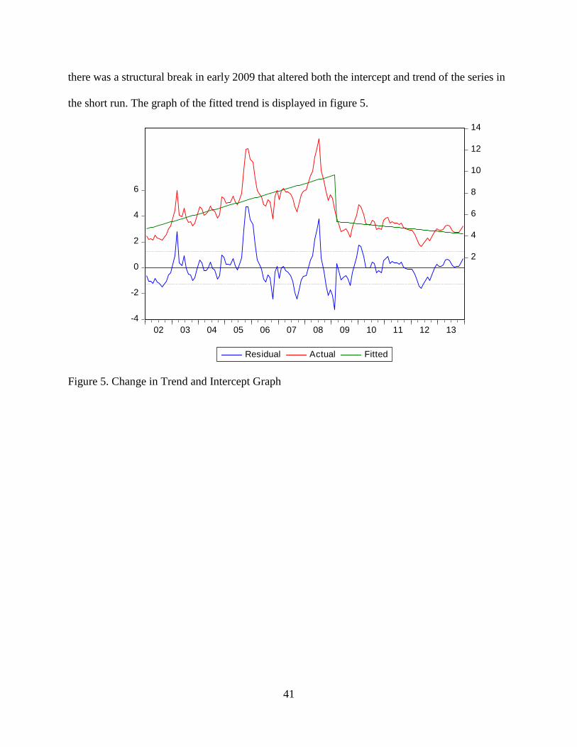
41
there was a structural break in early 2009 that altered both the intercept and trend of the series in
the short run. The graph of the fitted trend is displayed in figure 5.
Figure 5. Change in Trend and Intercept Graph
-4
-2
0
2
4
6
2
4
6
8
10
12
14
02 03 04 05 06 07 08 09 10 11 12 13
Residual Actual Fitted

42
ERROR CORRECTION MODEL
A variable is considered to be integrated d of order d (or I(d)) if it must be differenced “d-
times” in order for the variable to become stationary. If linear combination of two or more I(1)
variables are found to be stationary, a long-run relationship between the variables exists amongst
them and they are considered to be cointegrated (Engle and Granger; 1987). An important aspect
of cointegrated variables is that over time they are influenced by any deviation from the long-run
equilibrium. For the system to return to the long-run equilibrium, some variables must shift to
respond to the movement of the disequilibrium. Engle and Granger (1987) have proved that a
well-defined error correction mechanism (ECM) exists when two or more variables are
cointegrated. The ECM term explains the short-run adjustment that the cointegrated variables
must make in order to return to the long-run equilibrium. A Vector Error Correction (VEC)
model is appropriate for this study because the specification has an ECM built into it so that the
endogenous variables are restricted to their long-run relationship and allowed to make short-run
adjustments.
Using a Vector Error Correction (VEC) model, information can be obtained on the short-
run dynamics of the variables in a system. The VEC model used in this study consists of three
endogenous variables (natural gas price (NGP), oil price (OILP), and coal price (COALP)), with
one cointegrating vector based on the results of table 9, and eight exogenous variables (net
energy exports (EEXP), GDP per capita (GDPPC), US dollar index (USD), Dow Jones Industrial
Average (DOW), natural gas from fracking (FRACK), trend, change in trend (T2), and change in
intercept (C2)). The two equations of the VEC are:

43
(Eq. 7)
( ) ∑
∑
∑
( ) ∑
∑
∑
( ) ∑
∑
∑
where t is years, i is the number of lags, and , are parameters to be estimated,
and , j=1, are estimated parameters from the cointegration vectors, and are errors.
The errors and all of the terms involving , are stationary.
Thus, the linear combination of the lagged variables ( )
must be stationary and represent the long-run equilibrium among the two variables. In this model
there is only one error correction term that corresponds to the cointegration vector. In the long-
run equilibrium the error correction term will equal zero, but if NGP, OILP, and COALP break
from the long-run equilibrium, the error correction term will be nonzero and each variable will
adjust to reestablish the equilibrium relation. Finally, the coefficient measures the speed at
which the k-th endogenous variable adjusts toward equilibrium based on the cointegration vector
j, j=1.

44
ERROR CORRECTION RESULTS
The Vector Error Correction (VEC) model can be viewed in table 12. Although the VEC
model displays outputs for the three endogenous variables, natural gas price, oil price, and coal
price, the primary endogenous variable of interest is natural gas price. Note that the R2
is low, so
it explains only about 27 percent of the variation in the price of natural gas. This indicates that
there are factors outside the scope of this study affecting the monthly fluctuations in the price of
natural gas, potentially well reserves or the number of heating and cooling days in the year. The
VEC model explains historical price changes and allows forecasting of natural gas price
movements after exogenous shocks.

45
Table 12. Error Correction Results
The underlying dynamic price relationships affecting the movements of natural gas price
are of primary interest. The impact of changes in natural gas prices from the previous month, t-1,
is significant and positive indicating that a 10 percent increase in the previous month’s natural
gas price causes a 2.7 percent increase in the current month’s natural gas price. The US dollar
Explanatory Variables Equation
Δ(NGP) Δ(OILP) Δ(COALP)
CointEq1 -0.007647 0.151661*** 0.002422
[-0.28705] [ 8.96859] [ 0.09849]
Δ(NGP(-1)) 0.276012** 0.028467 0.196495*
[ 2.23869] [ 0.36373] [ 1.72649]
Δ(OILP(-1)) -0.132675 0.312543*** 0.200353*
[-1.00867] [ 3.74320] [ 1.65009]
Δ(COALP(-1)) -0.20522 0.008912 -0.322049***
[-1.58613] [ 0.10851] [-2.69645]
C 1.646279 32.89157*** 6.708674
[ 0.16897] [ 5.31829] [ 0.74593]
Trend -0.00303 -0.003902 0.002793
[-0.65118] [-1.32088] [ 0.65020]
C2 -0.599247 1.935409*** 0.418366
[-0.84120] [ 4.27994] [ 0.63621]
T2 0.007458 -0.018742*** -0.004114
[ 0.96851] [-3.83409] [-0.57871]
EEXP 0.086415 0.060701 -0.012563
[ 1.04560] [ 1.15704] [-0.16467]
GDPPC -0.511765 3.650799*** 0.429185
[-0.51566] [ 5.79497] [ 0.46847]
USD -0.775266* -0.791794*** -0.755209*
[-1.70109] [-2.73692] [-1.79512]
DOW -0.076454 0.657362*** 0.18948
[-0.31874] [ 4.31731] [ 0.85575]
FRACK -0.18861* 0.096794 -0.09304
[-1.69758] [ 1.37242] [-0.90716]
R-squared 0.274934 0.730351 0.36732
Adj. R-squared 0.152388 0.684777 0.260388

46
index was negative and significant at the 10 percent level. This index is a weighted geometric
mean of the US dollar’s value relative to a batch of foreign currencies: euro, yen, pound,
Canadian dollar, Krona, and the Swiss franc. These results imply that a ten point increase in the
US dollar index causes a 7.7 percent drop in the price of natural gas. Since 1957, the US has
been a net importer of natural gas which means that a stronger dollar decreases the relative cost
of imports. Natural gas produced from fracking was also shown to be significant and implies that
a 10 percent increase in shale gas production from fracking decreases the current price of natural
gas by 1.8 percent.
The coefficient of the long-run adjustment equation identified by the cointegration tests
indicate that there is not long term adjustment in natural gas price when exogenous shocks affect
the relationship among the three endogenous variables. The coefficient for the cointegrating
equation is insignificant and negative, indicating that natural gas prices responds negatively
when oil and coal prices diverge from their long-run cointegrating relationship.
Finally, impulse response graphs were generated to observe the reaction of the fossil fuel
prices to endogenous shocks. The results from the impulse response functions are presented in
figure 6. The graphs show that natural gas price responds positively to a positive shock in its own
price. Natural gas responds negatively to a positive shock in oil price in the first two months,
and then becomes and remains negative after 12 months. Lastly, natural gas price responds
negatively to a positive shock in coal prices before staying negative after 8 months. The impulse
response functions show how the price of natural gas does not move back to the original price
given a one standard deviation shock to any of the three prices, and this helps explain the
insignificance of the cointegrating equation for natural gas in the ECM.

47
Figure 6. Impulse Response Functions
-.04
.00
.04
.08
.12
2 4 6 8 10 12 14 16 18 20 22 24
Response of NGP to NGP
-.04
.00
.04
.08
.12
2 4 6 8 10 12 14 16 18 20 22 24
Response of NGP to OILP
-.04
.00
.04
.08
.12
2 4 6 8 10 12 14 16 18 20 22 24
Response of NGP to COALP
-.02
.00
.02
.04
.06
2 4 6 8 10 12 14 16 18 20 22 24
Response of OILP to NGP
-.02
.00
.02
.04
.06
2 4 6 8 10 12 14 16 18 20 22 24
Response of OILP to OILP
-.02
.00
.02
.04
.06
2 4 6 8 10 12 14 16 18 20 22 24
Response of OILP to COALP
.00
.02
.04
.06
.08
2 4 6 8 10 12 14 16 18 20 22 24
Response of COALP to NGP
.00
.02
.04
.06
.08
2 4 6 8 10 12 14 16 18 20 22 24
Response of COALP to OILP
.00
.02
.04
.06
.08
2 4 6 8 10 12 14 16 18 20 22 24
Response of COALP to COALP
48
CONCLUSIONS
The United States (US) obtains 27% of its energy from natural gas, 35% from petroleum,
and 18% from coal which makes fossil fuels the primary energy sources consumed in the country
(EIA Annual Energy Outlook, 2014). Due to this large interdependence of fossil fuels, this study
estimated demand equations simultaneously for all three energy commodities. Instead of
focusing strictly on recent observations, long run relationships among energy commodities were
investigated using annual data covering 1918 through 2013. The 95 years of data incorporates
early periods of technological development and significant price volatility. Directed Acyclic
graphs were used for the first time to show precisely the causal relationship among fossil fuels,
and illustrated the endogeneity issue between the selected variables.
Due to the endogeneity problem of the data set, the findings from the Granger Causality
test, weak exogeneity test, and DAGs supported the use of the Seeming Unrelated Regression
method. The SUR model demonstrated that there was substitutability among fossil fuels, but the
small magnitude of the substitution indicates that demand for natural gas, oil, and coal are
independent of each other within the US market. The results found that lagged natural gas
demand, GDP per capita, natural gas price, oil price, and the Iranian oil shock were all
significant factors in determining natural gas demand over the past 95 years. Natural gas was
found to be a normal good that is income inelastic, and also a weak substitute with oil. The
analysis of these three fossil fuels together allowed for a more accurate model of the dynamic
energy market in the United States.
The short run price analysis of fossil fuel prices in the US market between 2007 and 2013
captured the large structural break between natural gas and oil prices. The model indicated that
the price of natural gas did not share a long run cointegrating price relationship with oil and coal.

49
This finding was supported by the long run analysis that showed the independent demand
structures of fossil fuels. The ECM did show that the price of natural gas is significantly affected
by the prior month’s natural gas price. The natural gas price was also significantly affected by
the strength of the US dollar which indicates that a strong dollar decreases the domestic price of
natural gas. Finally, natural gas from fracking was shown to have a significant negative affect on
the price of natural gas.
It is interesting to note the lack of a lag structure for the three prices. This possibly could
be due to large amounts of speculation in the energy market. One major issue with the model is
the low explanatory power of the natural gas equation which indicates that volatility in natural
gas price is being caused by variables outside the scope of this study. The impulse response
functions show that a one standard deviation shock to oil and coal prices has a dynamic and
permanent negative effect on the price of natural gas. This result potentially is capturing the
structural break in 2009.
While this study analyzes both the long and short term aspects of the US fossil fuel
market, there is room for future research. Since the R2
for the monthly natural gas price equation
was so low, further study into short term causes of natural gas price is nedcessary. Given that
energy prices can be heavily affected by the weather, future models may include adjustments for
fluctuations in temperature, possible weather shocks, and other short term price shocks.

50
BIBLIOGRAPHY
Al-Jarri, AS, and RA Startzman. "Worldwide Petroleum-Liquid Supply and Demand (Includes
Associated Papers 52597 and 52598)." Journal of Petroleum Technology 49, no. 12
(1997): 1,329-1,38.
Al‐Faris, A. "The Determinants of Crude Oil Price Adjustment in the World Petroleum
Market."OPEC review 15, no. 3 (1991): 215-28.
Bacon, Robert. "Modelling the Price of Oil." Oxford Review of Economic Policy (1991): 17-34.
Bartlett, Albert A. "An Analysis of Us and World Oil Production Patterns Using Hubbert-Style
Curves." Mathematical Geology 32, no. 1 (2000): 1-17.
Bessler, David A, and Jian Yang. "The Structure of Interdependence in International Stock
Markets." Journal of international money and finance 22, no. 2 (2003): 261-87.
Campbell, Colin J, and Jean H Laherrère. "The End of Cheap Oil." Scientific American 278, no.
3 (1998): 60-5.
Carter, Susan B, Scott S Gartner, Michael R Haines, Alan L Olmstead, Richard Sutch, and
Gavin Wright. "Historical Statistics of the United States: Millennial Edition."
Cambridge: Cambridge University Press, 2006.
Chickering, David Maxwell. "Optimal Structure Identification with Greedy Search." The
Journal of Machine Learning Research 3 (2003): 507-54.
EIA. 2014. Retrieved May 11, 2014 from Energy Information Agency: htpp://www.eia.gov
Chow, Gregory C. "Tests of Equality between Sets of Coefficients in Two Linear
Regressions."Econometrica: Journal of the Econometric Society (1960): 591-605.
51
Dees, Stéphane, Pavlos Karadeloglou, Robert K Kaufmann, and Marcelo Sanchez. "Modelling
the World Oil Market: Assessment of a Quarterly Econometric Model." Energy
Policy 35, no. 1 (2007): 178-91.
Deffeyes, Kenneth S. "World's Oil Production Peak Reckoned in near Future." Oil & gas
journal100, no. 46 (2002): 46-48.
Dickey, David A, and Wayne A Fuller. "Distribution of the Estimators for Autoregressive Time
Series with a Unit Root." Journal of the American statistical association 74, no. 366a
(1979): 427-31.
EIA, US. "Annual Energy Outlook 2013." US Energy Information Administration, Washington,
DC(2013).
Engle, Robert F, and Byung Sam Yoo. "Forecasting and Testing in Co-Integrated
Systems."Journal of econometrics 35, no. 1 (1987): 143-59.
Hamilton, James D. "Historical Oil Shocks." National Bureau of Economic Research, 2011.
Holditch, S, K Perry, and J Lee. "Unconventional Gas Reservoirs—Tight Gas, Coal Seams, and
Shales, Working Document of the National Petroleum Council on Global Oil and Gas
Study."National Petroleum Council (2007).
Hubbert, Marion King. "Energy Resources: A Report to the Committee on Natural Resources of
the National Academy of Sciences--National Research Council." National Academy of
Sciences-National Research Council, Washington, DC (USA), 1962.
———. Nuclear Energy and the Fossil Fuels. Vol. 95: Shell Development Company,
Exploration and Production Research Division Houston, TX, 1956.
Ivanhoe, LF. "Future World Oil Supplies: There Is a Finite Limit." World Oil 216 (1995): 77-
77.

52
Johansen, Søren. "Estimation and Hypothesis Testing of Cointegration Vectors in Gaussian
Vector Autoregressive Models." Econometrica: Journal of the Econometric
Society (1991): 1551-80.
Johansen, Søren, and Katarina Juselius. "Identification of the Long-Run and the Short-Run
Structure an Application to the Islm Model." Journal of Econometrics 63, no. 1 (1994):
7-36.
Kaufmann, Robert K, and Cutler J Cleveland. "Oil Production in the Lower 48 States:
Economic, Geological, and Institutional Determinants." Energy Journal 22, no. 1 (2001).
Kaufmann, Robert K, Stephane Dees, Pavlos Karadeloglou, and Marcelo Sanchez. "Does Opec
Matter? An Econometric Analysis of Oil Prices." The Energy Journal (2004): 67-90.
Kennedy, Michael. "An Economic Model of the World Oil Market." The Bell Journal of
Economics and Management Science (1974): 540-77.
King, Robert F, and David Morehouse. "Drilling Sideways—a Review of Horizontal Well
Technology and Its Domestic Application." Gas Energy Review 21 (1993): 21-28.
Klett, Timothy R, Donald L Gautier, and Thomas S Ahlbrandt. "An Evaluation of the Us
Geological Survey World Petroleum Assessment 2000." AAPG bulletin 89, no. 8 (2005):
1033-42.
Kolb, Robert W. The Natural Gas Revolution: At the Pivot of the World's Energy Future:
Pearson Education, 2013.
Krichene, Noureddine. "World Crude Oil and Natural Gas: A Demand and Supply
Model." Energy Economics 24, no. 6 (2002): 557-76.

53
Lauritzen, Steffen L, and Thomas S Richardson. "Chain Graph Models and Their Causal
Interpretations." Journal of the Royal Statistical Society: Series B (Statistical
Methodology)64, no. 3 (2002): 321-48.
Li, Yarui, Joshua D Woodard, and David J Leatham. "Causality among Foreign Direct
Investment and Economic Growth: A Directed Acyclic Graph Approach." Journal of
Agricultural and Applied Economics 45, no. 04 (2013).
Nashawi, Ibrahim Sami, Adel Malallah, and Mohammed Al-Bisharah. "Forecasting World
Crude Oil Production Using Multicyclic Hubbert Model." Energy & Fuels 24, no. 3
(2010): 1788-800.
Oil, Technically Recoverable Shale. "Shale Gas Resources: An Assessment of 137 Shale
Formations in 41 Countries Outside the United States." URL: http://www. eia.
gov/analysis/studies/worldshalegas (2013).
Pearl, Judea. "Causal Diagrams for Empirical Research." Biometrika 82, no. 4 (1995): 669-88.
———. "Fusion, Propagation, and Structuring in Belief Networks." Artificial intelligence 29,
no. 3 (1986): 241-88.
Perron, Pierre. "The Great Crash, the Oil Price Shock, and the Unit Root
Hypothesis."Econometrica: Journal of the Econometric Society (1989): 1361-401.
Roh, Jae-Whak, and David A Bessler. "Occupant Death: A Study with Directed
Graphs." Applied Economics Letters 6, no. 5 (1999): 303-06.
Ryan, JM. "Limitations of Statistical Methods for Predicting Petroleum and Natural Gas
Reserves and Availability." Journal of Petroleum Technology 18, no. 03 (1966): 281-87.
Scheines, Richard, Peter Spirtes, Clark Glymour, and Christopher Meek. Tetrad IV: Users
Manual: Lawrence Erlbaum Associates, Hillsdale, NJ, 1994.

54
Sorrell, Steve, Richard Miller, Roger Bentley, and Jamie Speirs. "Oil Futures: A Comparison of
Global Supply Forecasts." Energy Policy 38, no. 9 (2010): 4990-5003.
Sorrell, Steve, and Jamie Speirs. "Hubbert’s Legacy: A Review of Curve-Fitting Methods to
Estimate Ultimately Recoverable Resources." Natural resources research 19, no. 3
(2010): 209-30.
Spirtes, Peter, Clark N Glymour, and Richard Scheines. Causation, Prediction, and Search. Vol.
81: MIT press, 2000.
Strahan, David. The Last Oil Shock: A Survival Guide to the Imminent Extinction of Petroleum
Man: John Murray, 2008.
Szklo, Alexandre, Giovani Machado, and Roberto Schaeffer. "Future Oil Production in Brazil—
Estimates Based on a Hubbert Model." Energy policy 35, no. 4 (2007): 2360-67.
Yahoo Finance. 2014. Retrieved May 11, 2014 from Yahoo: http://finance.yahoo.com
YCharts. 2014. Retrieved May 11, 2014 from YCharts: http://www.ycharts.com
Yearbook 1949-1975, Minerals. "Bureau of Mines." United States Department of the Interior,
US Government Printing Office, Washington, DC (1971).
Zellner, Arnold. "An Efficient Method of Estimating Seemingly Unrelated Regressions and
Tests for Aggregation Bias." Journal of the American statistical Association 57, no. 298
(1962): 348-68.