a heuristic approach to creating an annual delivery
TRANSCRIPT

A Heuristic Approach to Creating anAnnual Delivery Program for an LNGProducer with Transshipment
Ingrid Horpedal BuggeMaulisha Thavarajan
Industrial Economics and Technology Management
Supervisor: Peter Schütz, IØTCo-supervisor: Ruud Egging, IØT
Department of Industrial Economics and Technology Management
Submission date: June 2018
Norwegian University of Science and Technology


Purpose of Master’s Thesis
The purpose of this thesis is to create an Annual Delivery Program (ADP) foran LNG producer and its customers. The ADP describes delivery schedules tocustomers located in different continents. Due to limited availability of routesfrom the producer to the customers, the cargo can be delivered either directly orvia a transshipment port.
The deliveries are determined based on annual demand stated in long-term con-tracts. The annual demand must be fulfilled for each long-term customer andis further divided into periodic demand. The periodic demand allows over- andunder-deliveries. Both over- and under-delivery are penalized. Excess LNG can besold in the spot market.
The producer seeks to minimize the costs of operation when fulfilling the long-term contracts. Selling LNG in the spot market can be considered as a negativecost. In addition, inventory constraints are considered at the producer and thetransshipment port. The problem of creating an ADP can be categorized as aMaritime Inventory Routing Problem (MIRP).
MIRPs are difficult to solve. So far in the existing literature, similar problems havebeen solved with exact methods and heuristics. Heuristics are able to solve largerinstances and provide good solutions. This thesis therefore focus on heuristics inorder to create an ADP.
i

ii

Preface
This Master’s thesis is the concluding work of our Master of Science at the Norwe-gian University of Science and Technology. Our field of specialization is ManagerialEconomics and Operations Research at the Department of Industrial Economicsand Technology Management.
This thesis was written during the spring semester of 2018 and is a continuationof our specialization work from the fall semester of 2017 (Bugge and Thavarajan,2017).
We would like to express our deepest gratitude to our supervisors, Peter Schutzand Ruud Egging, for excellent feedback and guidance. We appreciate your sincereenthusiasm towards the thematics in the thesis. The thesis has been written incooperation with Tieto, and we would like to thank Jørgen Glomvik Rakke foractively contributing with his insights, and Lars Petter Bjørgen for his valuableinputs.
Trondheim, June 11th, 2018
Ingrid Horpedal Bugge Maulisha Thavarajan
iii

iv
Abstract
In this thesis, an Annual Delivery Program (ADP) planning problem is studied.The objective of the ADP planning problem is to create a cost-efficient deliveryschedule for a liquefied natural gas (LNG) producer, who has a fleet of heteroge-neous vessels. The fleet of vessels consists of ice-going vessels and conventionalvessels. The LNG producer has entered long-term contracts with customers indifferent parts of the world, and is committed to fulfill the demands stated in thecontracts.
Voyages to the customers are either direct or via a transshipment port. The directvoyages to the customers in Asia depend on the opening periods of the NorthernSea Route. If the NSR is closed, the ice-going vessels travel to the transshipmentport to transfer the cargo onto a conventional vessel, which then continues thejourney via the Suez Canal. Only ice-going vessels are permitted to use the NSR.
The size of the storage tank at the transshipment port is a challenging factor inthe ADP planning problem, and thus partial loading is implemented to avoid abottleneck caused by residual LNG left in the tank. Partial loading only appliesto the ice-going vessels sent from the producer’s port, and the filling levels in thevessel tanks are regulated to reduce the effects of sloshing.
The ADP planning problem can be classified as an industrial shipping problemwith decision making on a tactical planning level. Relevant literature is presentedto illustrate how certain properties of the problem, such as partial loading, isimplemented in other works, and how different solution methods have been usedto solve LNG inventory routing problems (LNG-IRP). The ADP planning problemis a maritime inventory routing problem (MIRP). MIRPs are numerically complexto solve and usually require heuristic solution methods to produce good solutions.
A mixed integer programming (MIP) formulation of the ADP planning problemis developed based on the aforementioned factors, where partial loading and boil-off considerations are explicitly handled in the model formulation for some of thevessels.
Because of the long planning horizon of the ADP planning problem, a rollinghorizon heuristic (RHH) is proposed to solve the problem. Several strategies forthe different periods within a sub-horizon are tested to solve the ADP planning
v

problem efficiently. In addition to the RHH, an aggregation and disaggregationheuristic (ADH) is proposed as an alternative approach to solving a reduced size ofthe problem. The intention behind both methods is to reduce the complexity of theproblem during the solution process, by either solving the problem in shorter sub-horizons or by reducing the number of nodes in the network. The solution methodsare combined to create an ADP quickly. Results from these solution methods arecompared with a solution from a corresponding case solved by exact method.
The RHH obtains the best result for the ADP planning problem. The heuristicimproves both the ADP-objective and computational time compared to the exactsolution method. When the ADH is combined with the RHH to solve the aggregatedcase, the computational time can be decreased further. Despite the improvedsolution time, the RHH-ADH did not improve the solution compared with theexact solution method.
The results show that the performance of the ADH depends on several factors; thechosen aggregation strategy, the solution method used for solving the aggregatedcase, and the amount of over- and under-deliveries in the solution for the aggregatedcase.
vi

Sammendrag
Denne masteroppgaven omhandler et arlig leveringsprogram–planleggingsproblem(ADP-planleggingsproblem). Malet med et slikt problem er a lage en kostnadsef-fektiv leveringsplan for en flytende naturgassprodusent (LNG-produsent) som haren heterogen flate. Flaten bestar av isgaende skip og konvensjonelle skip. LNG-produsenten har inngatt langtidskontrakter med kunder over hele verden, og erforpliktet til a tilfredsstille etterspørselen som er spesifisert i kontraktene.
En sjøreise kan enten ga direkte til kundene eller via en omlastningshavn til kun-dene. Direkteturer til kunder i Asia avhenger av apningstidene til den nordligesjørute (NSR). Dersom NSR er stengt ma de isgaende skipene reise til omlastning-shavnen for a overføre last til konvensjonelle skip. De konvensjonelle skipene fort-setter seilasen til Asia gjennom Suez-kanalen. Det kun er tillatt a bruke isgaendeskip i NSR.
Størrelsen pa lagertanken i omlastningshaven er en utfordring i ADP- planleg-gingsproblemet. Delvis lasting er innført for a unnga en flaskehals-problematikksom skyldes gjenværende mengder av LNG i lagertanken. Delvis lastning er kunaktuelt for de isgaende skipene som seiler mellom produsenten og omlastningshav-nen. Selv om skipene kan lastes delvis kreves det at mengden last ombord er overet minimumskrav for a redusere effektene av sloshing.
ADP-planleggingsproblemet kan klassifiseres som et industrielt skipsfartsproblem,med beslutningstaking innenfor en taktisk planleggingshorisont. Relevant litteraturer presentert for a illustrere hvordan visse aspekter av problemet er implementerti annen litteratur. I tillegg er det ønskelig a vise hvordan ulike løsningsmetoder erbenyttet for a løse kombinerte LNG lagerstyrings- og ruteplanleggingsproblemer.ADP-planleggingsproblemet er et kombinert maritimt lagerstyrings- og ruteplan-leggingsproblem (MIRP). MIRP er numerisk komplekse og krever ofte en heuristiskløsningsmetode for a kunne gi gode løsninger.
Et blandet heltallsprogram er formulert basert pa ADP-planleggingsproblemet.Denne formuleringen inkluderer tidligere nevnte faktorer, der delvis lastning ogavdamping av LNG er en eksplisitt del av modellformuleringen for noen av skipene.
Grunnet den lange planleggingshorisonten for ADP-planleggingsproblemet er enrullende horisont-heuristikk (RHH) foreslatt for a løse problemet. Flere strate-
vii

gier for de ulike periodene innenfor en sub-horisont er testet for a kunne fa eneffektiv løsningsprosess. I tillegg til RHH, er en aggregering og disaggregerings-heuristikk (ADH) utviklet for a løse en mindre instans av problemet. Intensjo-nen med begge metodene er a redusere kompleksiteten til problemet, enten veda løse det i mindre sub-horisonter eller ved a redusere antall noder i nettverket.Løsningsmetodene kombineres for a raskt kunne produsere en ADP. Resultatene frabegge løsningsmetoder sammenliknes med en løsning fra tilsvarende probleminstansløst med eksakt metode.
RHH gir de beste resultatene for ADP-planleggingsproblemet. Heuristikken forbedrerbade malfunksjonen til ADP og løsningstiden sammenliknet med eksakt metode.Dersom ADH kombineres med RHH (RHH-ADH) for a løse den aggregerte prob-leminstansen, kan løsningstiden reduseres ytterligere. Til tross for en forbedretløsningstid gir ikke RHH-ADH en bedre løsningsverdi sammenliknet med den ek-sakte løsningsmetoden.
Ytelsen til ADH avhenger av flere faktorer; valg av aggregeringsstrategi, løsningsmetodebrukt for a løse den aggregerte probleminstansen, og mengden over- og underlev-ering i løsningen til den aggregerte instansen.
viii

Contents
1 Introduction 1
2 Background 52.1 LNG Market . . . . . . . . . . . . . . . . . . . . . . . . . . . . . . . 5
2.1.1 Imports . . . . . . . . . . . . . . . . . . . . . . . . . . . . . . 62.1.2 Exports . . . . . . . . . . . . . . . . . . . . . . . . . . . . . . 7
2.2 Value Chain . . . . . . . . . . . . . . . . . . . . . . . . . . . . . . . . 82.3 Contracts and Trading . . . . . . . . . . . . . . . . . . . . . . . . . . 9
2.3.1 Short-term Trading . . . . . . . . . . . . . . . . . . . . . . . . 92.4 Annual Delivery Program . . . . . . . . . . . . . . . . . . . . . . . . 102.5 Arctic LNG . . . . . . . . . . . . . . . . . . . . . . . . . . . . . . . . 11
2.5.1 The Northern Sea Route and Vessels . . . . . . . . . . . . . . 122.5.2 Storage Limitations at the Transshipment Port . . . . . . . . 13
3 Literature Review 153.1 Shipping Modes . . . . . . . . . . . . . . . . . . . . . . . . . . . . . . 153.2 Planning Levels . . . . . . . . . . . . . . . . . . . . . . . . . . . . . . 163.3 Annual Delivery Program . . . . . . . . . . . . . . . . . . . . . . . . 183.4 Partial Loading . . . . . . . . . . . . . . . . . . . . . . . . . . . . . . 193.5 Transshipment . . . . . . . . . . . . . . . . . . . . . . . . . . . . . . 213.6 Solution Methods . . . . . . . . . . . . . . . . . . . . . . . . . . . . . 21
4 Problem Description 234.1 The ADP Planning Problem . . . . . . . . . . . . . . . . . . . . . . . 234.2 Seasonal Routes and Vessels . . . . . . . . . . . . . . . . . . . . . . . 254.3 LNG Cargo and Partial Loading . . . . . . . . . . . . . . . . . . . . 26
4.3.1 Boil-off . . . . . . . . . . . . . . . . . . . . . . . . . . . . . . 264.3.2 Partial Loading . . . . . . . . . . . . . . . . . . . . . . . . . . 26
5 Mathematical Model 295.1 Assumptions . . . . . . . . . . . . . . . . . . . . . . . . . . . . . . . 295.2 Notation . . . . . . . . . . . . . . . . . . . . . . . . . . . . . . . . . . 305.3 Model Description . . . . . . . . . . . . . . . . . . . . . . . . . . . . 325.4 Model Formulation . . . . . . . . . . . . . . . . . . . . . . . . . . . 36
6 Solution Methods 39
ix

CONTENTS
6.1 Rolling Horizon Heuristic . . . . . . . . . . . . . . . . . . . . . . . . 396.2 Aggregation and Disaggregation Heuristic . . . . . . . . . . . . . . . 42
6.2.1 Description of Disaggregation Procedure . . . . . . . . . . . . 446.2.2 Discussion . . . . . . . . . . . . . . . . . . . . . . . . . . . . . 45
7 Input Data 477.1 Ports . . . . . . . . . . . . . . . . . . . . . . . . . . . . . . . . . . . . 477.2 Vessels . . . . . . . . . . . . . . . . . . . . . . . . . . . . . . . . . . . 49
7.2.1 Traveling Time . . . . . . . . . . . . . . . . . . . . . . . . . . 497.2.2 Operative Costs . . . . . . . . . . . . . . . . . . . . . . . . . 507.2.3 Boil-off . . . . . . . . . . . . . . . . . . . . . . . . . . . . . . 51
7.3 Penalty Costs . . . . . . . . . . . . . . . . . . . . . . . . . . . . . . . 527.4 Planning Horizon and Initial Values . . . . . . . . . . . . . . . . . . 53
8 Computational Study 558.1 Rolling Horizon Heuristic Settings . . . . . . . . . . . . . . . . . . . 558.2 Full Case . . . . . . . . . . . . . . . . . . . . . . . . . . . . . . . . . 59
8.2.1 Exact Method . . . . . . . . . . . . . . . . . . . . . . . . . . 598.2.2 Rolling Horizon Heuristic . . . . . . . . . . . . . . . . . . . . 61
8.3 Aggregated Case . . . . . . . . . . . . . . . . . . . . . . . . . . . . . 658.3.1 Aggregation Strategies . . . . . . . . . . . . . . . . . . . . . . 668.3.2 ADH . . . . . . . . . . . . . . . . . . . . . . . . . . . . . . . . 71
8.4 Comparison of Solution Methods . . . . . . . . . . . . . . . . . . . . 75
9 Concluding Remarks 79
10 Future Research 81
Bibliography 83
Appendices 89
A Derivation of Boil-Off Constraints 91
B Graphs Showing Monthly Over- and Under-deliveries 95B.1 RHH Full Case . . . . . . . . . . . . . . . . . . . . . . . . . . . . . . 95B.2 Aggregated Case . . . . . . . . . . . . . . . . . . . . . . . . . . . . . 96B.3 E-ADH After Post-processing . . . . . . . . . . . . . . . . . . . . . . 97B.4 RHH-ADH After Post-processing . . . . . . . . . . . . . . . . . . . . 98
x

List of Figures
2.1 Overview of global net imports in 2017 . . . . . . . . . . . . . . . . . 62.2 Overview of global net exports in 2017 . . . . . . . . . . . . . . . . . 72.3 The LNG value chain . . . . . . . . . . . . . . . . . . . . . . . . . . 82.4 Spot and short-term trade in recent years . . . . . . . . . . . . . . . 102.5 Map of the routes . . . . . . . . . . . . . . . . . . . . . . . . . . . . . 12
4.1 Penalty costs as a function of deviations in volume. . . . . . . . . . . 244.2 Overview of routes and vessels . . . . . . . . . . . . . . . . . . . . . 26
6.1 The rolling horizon heuristic . . . . . . . . . . . . . . . . . . . . . . . 406.2 Overview of the Aggregation Disaggregation Heuristic . . . . . . . . 43
8.1 End of central period-problem at the transshipment port . . . . . . . 588.2 Annual deviations from the 13-months instance and 14-months in-
stance . . . . . . . . . . . . . . . . . . . . . . . . . . . . . . . . . . . 618.3 Annual deviation obtained for the full case with the rolling horizon
heuristic . . . . . . . . . . . . . . . . . . . . . . . . . . . . . . . . . . 628.4 Solutions obtained in the iterations in RHH . . . . . . . . . . . . . . 648.5 Aggregation Strategies . . . . . . . . . . . . . . . . . . . . . . . . . . 668.6 Annual deviation after ADH, given aggregation with Strategy 1 . . . 688.7 Annual deviation after ADH, given aggregation with Strategy 2 . . . 708.8 Annual deviation after ADH, given aggregation with Strategy 3 . . . 718.9 Annual deviation from E-ADH and RHH-ADH . . . . . . . . . . . . 728.10 Monthly deviations from E-ADH and RHH-ADH before destination
swap . . . . . . . . . . . . . . . . . . . . . . . . . . . . . . . . . . . . 738.11 Annual deviations after post-processing the ADH solutions . . . . . 74
B.1 Monthly deviations full case . . . . . . . . . . . . . . . . . . . . . . . 95B.2 Monthly deviations Strategy 1 . . . . . . . . . . . . . . . . . . . . . 96B.3 Monthly deviations Strategy 2 . . . . . . . . . . . . . . . . . . . . . 96B.4 Monthly deviations Strategy 3 . . . . . . . . . . . . . . . . . . . . . 97B.5 Monthly deviations E-ADH after post-processing . . . . . . . . . . . 97B.6 Monthly deviations RHH-ADH after post-processing . . . . . . . . . 98
xi

LIST OF FIGURES
xii

List of Tables
7.1 Conversion between units . . . . . . . . . . . . . . . . . . . . . . . . 477.2 Overview of ports and customers considered in the problem . . . . . 487.3 Operative Costs . . . . . . . . . . . . . . . . . . . . . . . . . . . . . . 507.4 Costs used for annual over- and under-deliveries . . . . . . . . . . . . 53
8.1 Tested strategies for RHH . . . . . . . . . . . . . . . . . . . . . . . . 568.2 Number of variables and constraints for the full case before and after
applying Presolve. . . . . . . . . . . . . . . . . . . . . . . . . . . . . 608.3 Results from solving the full case by exact methods. . . . . . . . . . 608.4 Results from the rolling horizon heuristic . . . . . . . . . . . . . . . 628.5 Time used in each iteration for RHH . . . . . . . . . . . . . . . . . . 638.6 Results from testing the aggregation strategies. . . . . . . . . . . . . 668.7 Solutions from the ADH without post-processing . . . . . . . . . . . 728.8 Solutions from the ADH before and after destination swaps . . . . . 748.9 Comparison of solution methods . . . . . . . . . . . . . . . . . . . . 75
xiii

Chapter 1
Introduction
The demand for liquefied natural gas (LNG) has increased significantly during thepast decade. In 2017, global imports peaked at 289.8 million tons (MT) (GIIGNL,2018). Natural gas is increasingly used as an energy source in electric power andindustrial sector, and emits almost half as much CO2 per unit of energy comparedto coal (EIA, 2017a,b). By converting natural gas to liquid state, the volume isreduced by a factor of 1:625, which enables the transportation of large amounts ofnatural gas more efficiently.
Increasing contribution from the supply side in recent years has motivated buyers topush for more flexibility in existing long-term contracts, such as more frequent re-negotiations on pricing terms, delivery quantities and destination flexibility (Gloys-tein, 2018). With new participants entering the demand side of the LNG markets,the demand side is becoming increasingly more diverse and complex.
In the capital intensive LNG industry, LNG producers typically enter contracts witha duration of around 20 years to minimize the risks from investment and guaranteereturn on the investments. But with a growing LNG demand and buyers pushingfor more flexibility, the traditional, rigid contracting schemes are now challengedby developments in short-term trades and sales in spot markets. More frequentre-negotiations on contractual terms may further complicate the delivery scheduleprocesses of the LNG producers.
The LNG producers usually plan the deliveries up to a year ahead. The result ofthe scheduling processes is an Annual Delivery Program (ADP), which is a deliveryschedule with a 12 month horizon. Since the producers are responsible for largeparts of the value chain, inventory constraints in different parts of the value chainare taken into account during scheduling to minimize idle capacities in the chainTusiani and Shearer (2007).
The scheduling processes have for a long time been carried out manually, mostlybased on experience and industry know-hows. Now that the changes in market
1

CHAPTER 1. INTRODUCTION
dynamics are confronting the traditional industry practices, LNG producers seethe monetary benefits in creating delivery schedules to satisfy the customer termsand at the same time, utilize central parts the LNG value chain.
Such a complex task necessitates the development of decision support tools thatcreate optimal delivery schedules with the above-mentioned factors in mind. It itcommon to create ADPs in-office during contract negotiations, and thus speed andquality are essential for such a decision support tool.
In this Master’s thesis, the goal is to develop a decision support tool that createsan ADP for an LNG producer situated in north of the Arctic Circle. Despite thechallenging arctic conditions, around 30% of undiscovered natural gas resources areexpected to be located within the Arctic Circle, making it an area of interest forLNG producers. Climate changes have lead to a reduction in sea ice levels overthe years, thus enabling longer navigation periods along the Northern Sea Route(NSR).
The LNG producer has entered long-term contracts with customers in Europe andAsia. The location of the production facilities enables the opportunity of using theNSR to reach the customers in Asia in a shorter amount of time.
Due to sea ice, navigation in the NSR is subject to strict regulations. This entailsthat vessels are permitted to sail along the route as long as they fulfill the technicalrequirements. The producer operates with heavily equipped, costly, ice-going ves-sels that fulfill these requirements. They are necessary to use along the ice-coveredparts of the routes. When the NSR is closed, the ice-going vessels need to use theconventional Suez route to reach the customers in Asia. To avoid using the ice-going vessels more than necessary, the producer has invested in a storage tank ata transshipment port in Europe to transfer cargo onto less expensive, conventionalvessels.
The ADP planning problem is an industrial shipping problem with a tactical plan-ning horizon, and falls under the category of maritime inventory routing problems(MIRPs). MIRPs are hard to solve due to the numerical complexity, and existingliterature on MIRPs and ADPs solve the problems with the use of exact methodsor heuristical approaches. The seasonal availability of NSR, voyages via a trans-shipment port and large distances between the producer and customers, introduceadditional complexity to the ADP planning problem. Therefore, in this Master’sthesis, we develop solution methods to improve the computational time of solvingthe ADP planning problem.
Rolling horizon heuristics have been applied in the existing ADP literature, andare able to solve scheduling problems with long time horizons efficiently. To theextent of our knowledge, aggregation and disaggregation techniques are not widelyused in recent MIRP literature. The combination of both solution methods is thusa novel twist to existing solution methods in the ADP literature.
2
The structure of the Master’s thesis is as following: in Chapter 2 several aspects ofthe LNG industry and the ADP planning problem are described, before reviewingexisting literature in Chapter 3. Chapter 4 presents a problem description of theADP planning problem, which is then formulated as a mathematical model inChapter 5. The two solution approaches that we use to solve the ADP planningproblem are described in 6. Relevant data and case instances are presented inChapter 7, before presenting the results and a discussion on the different solutionmethods in Chapter 8. Chapter 9 concludes the study we have carried out, andChapter 10 presents possible extensions for further research.
Due to a confidentiality agreement between the authors and Tieto, case specificdata and information are withheld from the thesis. Even though parts of the caseinstances and data have been constructed by the authors, these are omitted toavoid any implications.
3

CHAPTER 1. INTRODUCTION
4

Chapter 2
Background
Before introducing the ADP planning problem, an introduction to relevant conceptsfor the problem is presented in this chapter. Most of the information is based on thereport by Bugge and Thavarajan (2017) and has been adapted to this thesis. First,the current state of the LNG industry is presented in Chapter 2.1. An overview ofthe LNG value chain is then presented in Chapter 2.2. Contracts and developmentsin short-term trade play an important part in the trading aspect and are discussedin Chapter 2.3, before proceeding to ADPs in Chapter 2.4. Lastly, Chapter 2.5discusses the specific properties of the case and introduces challenges related to theADP planning problem.
2.1 LNG Market
There is an increasing demand in energy. The U.S. Energy Information Admin-istration (2017) presents an assessment on the developments of the global energymarkets based on a reference case with a timespan from 2015 to 2040. During thistime horizon, the report expects an increase of 28% in world energy consumption.Renewables turn out to be the fastest growing source of energy, with an increasein global consumption by 2.3% per year. Among the fossil fuels, natural gas isthe fastest growing energy source and is projected to increase by 1.4% annuallyin global consumption. Due to stable long-term economic growth in non-OECDcountries, these countries are expected to be the main drivers for the increasingenergy demand (EIA, 2017a).
5

CHAPTER 2. BACKGROUND
2.1.1 Imports
In 2017, the global LNG imports peaked at 289.8 million tons (MT), a substantialincrease from 263.6 MT the previous year. As shown below in Figure 2.1, theAsia-region has a 72.9% market share in global imports in 2017 and is drivingthe demand growth. Japan remains the leading importer of LNG, contributingwith a market share of 28.8% in 2017 (GIIGNL, 2018). China’s energy demandis changing. Air pollution is a serious problem in China, and the authorities aretrying to reduce the emissions. As of 2017, the Chinese Government imposed strictregulations known as the “2+26”-policy. The policy was enforced in the wintermonths of 2017 and 2018 and reduced the coal consumption, which is a majorenergy source in both industrial and private sector (Tremblay, 2017). The countrychose to rely more on LNG imports. In fact, GIIGNL (2018) reports an increase inthe country’s imports by 42.3% in 2017, thus overtaking the position as the secondleading importing country of LNG in Asia from South Korea. Since LNG as anenergy source has lower CO2 emissions compared to coal and other fossil fuels, itis not unlikely that the demand for LNG will increase in the future, especially forChina (EIA, 2017b). In Europe, the net LNG imports increased by 7.5 MT mainlydue to increased demand for power generation (GIIGNL, 2018).
Figure 2.1: Overview of global net imports in 2017. Based on data from GIIGNL (2018).
6

2.1. LNG MARKET
2.1.2 Exports
GIIGNL (2018) reports 2017 as the year with the strongest supply growth since2010, with 289.8 MT in global exports. The number of exporting countries in-creased to 20, and a total of five new onshore liquefaction trains were commissionedin Australia, the US, and Russia. Australia increased the global LNG supply by10.7 MT, while the US contributed with an additional 9.6 MT. Qatar has been aleading exporter of LNG for several years. In 2017, the country supplied 26.7% ofglobal LNG, compared to 30% from the previous year, due to maintenance. TheUS has increased its export as a result of new liquefaction plants coming online andsupplied 25 countries in 2017, compared to 13 in the previous year. Following theinitiations of new projects in 2016, Australia remains the second largest LNG ex-porter globally, contributing with 55.56 MT in 2017, an increase by 10.7 MT fromthe previous year. With the initiation of the first of three new trains in Russia,the country stood for 11.49 MT in 2017. The report is expecting an increase inthe supply share from the Atlantic Basin, mainly due to the initiation of severalprojects in the US.
Figure 2.2: Overview of global net exports in 2017. Based on data from GIIGNL (2018).
7
CHAPTER 2. BACKGROUND
2.2 Value Chain
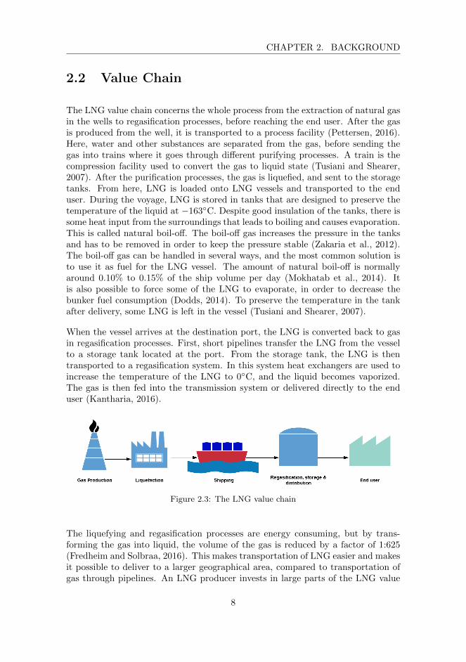
The LNG value chain concerns the whole process from the extraction of natural gasin the wells to regasification processes, before reaching the end user. After the gasis produced from the well, it is transported to a process facility (Pettersen, 2016).Here, water and other substances are separated from the gas, before sending thegas into trains where it goes through different purifying processes. A train is thecompression facility used to convert the gas to liquid state (Tusiani and Shearer,2007). After the purification processes, the gas is liquefied, and sent to the storagetanks. From here, LNG is loaded onto LNG vessels and transported to the enduser. During the voyage, LNG is stored in tanks that are designed to preserve thetemperature of the liquid at −163◦C. Despite good insulation of the tanks, there issome heat input from the surroundings that leads to boiling and causes evaporation.This is called natural boil-off. The boil-off gas increases the pressure in the tanksand has to be removed in order to keep the pressure stable (Zakaria et al., 2012).The boil-off gas can be handled in several ways, and the most common solution isto use it as fuel for the LNG vessel. The amount of natural boil-off is normallyaround 0.10% to 0.15% of the ship volume per day (Mokhatab et al., 2014). Itis also possible to force some of the LNG to evaporate, in order to decrease thebunker fuel consumption (Dodds, 2014). To preserve the temperature in the tankafter delivery, some LNG is left in the vessel (Tusiani and Shearer, 2007).
When the vessel arrives at the destination port, the LNG is converted back to gasin regasification processes. First, short pipelines transfer the LNG from the vesselto a storage tank located at the port. From the storage tank, the LNG is thentransported to a regasification system. In this system heat exchangers are used toincrease the temperature of the LNG to 0◦C, and the liquid becomes vaporized.The gas is then fed into the transmission system or delivered directly to the enduser (Kantharia, 2016).
Figure 2.3: The LNG value chain
The liquefying and regasification processes are energy consuming, but by trans-forming the gas into liquid, the volume of the gas is reduced by a factor of 1:625(Fredheim and Solbraa, 2016). This makes transportation of LNG easier and makesit possible to deliver to a larger geographical area, compared to transportation ofgas through pipelines. An LNG producer invests in large parts of the LNG value
8

2.3. CONTRACTS AND TRADING
chain, since the operations require production facilities, vessels, and receiving ter-minals. This leads to high investment costs, but the additional transportation costsare lower compared to the cost of pipelines. Therefore, LNG transportation is moreprofitable than pipelines (Pettersen, 2016).
2.3 Contracts and Trading
The LNG trade has for a long time been characterized by long-term contracts.There are mainly two types of contractual obligations: long-term and short-term.Long-term contracts have a duration of typically 5 to 20 years, while short-termcontracts typically last less than 5 years (International Gas Union, 2017). TheLNG-business is capital intensive due to high investment costs in facilities, equip-ment and vessels. By entering long-term contracts, the producers are secured moresteady cash-flows in a longer time horizon.
During negotiations, buyer and seller agree on a fixed volume of LNG to be deliv-ered annually, which is specified as an annual contractual quantity (ACQ) in thecontracts. However, the deliveries are not always met exactly. Differences in vesseltank capacities and maintenance are examples of how a producer might deviatefrom the ACQ. ACQs are normally specified as ”take-or-pay”, which means thatthe buyer is obligated to pay for the cargo to be delivered even if not taken. So, inthe unfortunate case where under-delivery occurs, i.e. due to plant maintenance,the buyer still pays for the shortfall. The producer would then have to deliver themissed volume later or the following year. When over-delivery occurs, for instanceas a result of improved plant performance, the contracts normally contain clausesthat specify which party has the preferential rights to claim the excess LNG. Over-delivery is profitable for buyer and seller (Tusiani and Shearer, 2007). Accordingto Gloystein (2018), most Asian long-term contracts state the destination of theLNG cargo explicitly, which would prevent Asian buyers from selling LNG, or morespecifically excess LNG, to third parties.
2.3.1 Short-term Trading
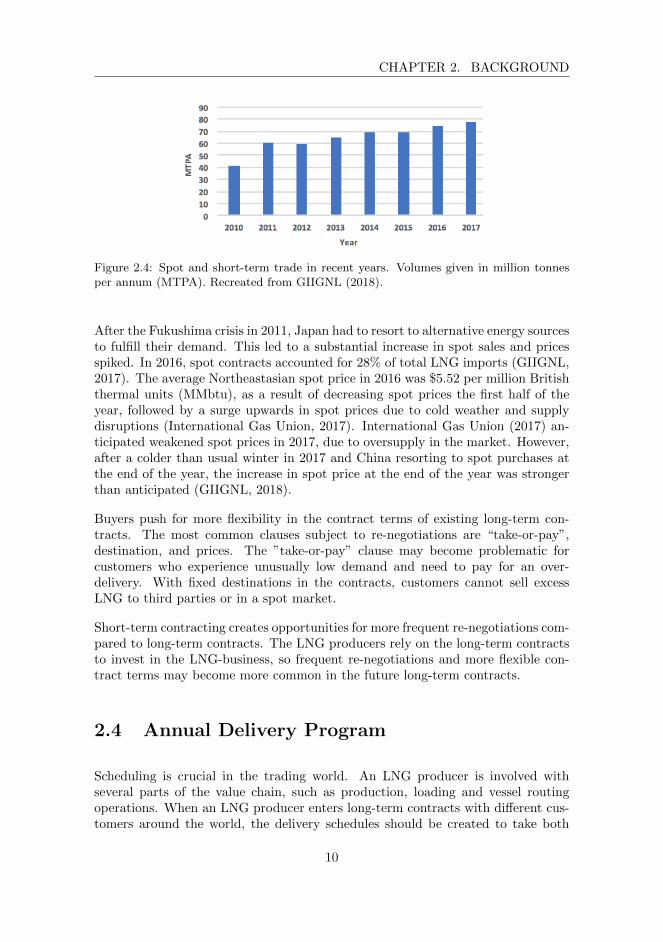
Sales in spot markets and contracts with short-term commitments have becomemore common in the past decade and challenge the traditional long-term contracts.Spot markets are characterized by the immediate trade of commodities or “tradeon the spot”. The price of the commodities is determined by the market. Figure2.4 shows the global spot and short-term trades in recent years.
9
CHAPTER 2. BACKGROUND
Figure 2.4: Spot and short-term trade in recent years. Volumes given in million tonnesper annum (MTPA). Recreated from GIIGNL (2018).
After the Fukushima crisis in 2011, Japan had to resort to alternative energy sourcesto fulfill their demand. This led to a substantial increase in spot sales and pricesspiked. In 2016, spot contracts accounted for 28% of total LNG imports (GIIGNL,2017). The average Northeastasian spot price in 2016 was $5.52 per million Britishthermal units (MMbtu), as a result of decreasing spot prices the first half of theyear, followed by a surge upwards in spot prices due to cold weather and supplydisruptions (International Gas Union, 2017). International Gas Union (2017) an-ticipated weakened spot prices in 2017, due to oversupply in the market. However,after a colder than usual winter in 2017 and China resorting to spot purchases atthe end of the year, the increase in spot price at the end of the year was strongerthan anticipated (GIIGNL, 2018).
Buyers push for more flexibility in the contract terms of existing long-term con-tracts. The most common clauses subject to re-negotiations are “take-or-pay”,destination, and prices. The ”take-or-pay” clause may become problematic forcustomers who experience unusually low demand and need to pay for an over-delivery. With fixed destinations in the contracts, customers cannot sell excessLNG to third parties or in a spot market.
Short-term contracting creates opportunities for more frequent re-negotiations com-pared to long-term contracts. The LNG producers rely on the long-term contractsto invest in the LNG-business, so frequent re-negotiations and more flexible con-tract terms may become more common in the future long-term contracts.
2.4 Annual Delivery Program
Scheduling is crucial in the trading world. An LNG producer is involved withseveral parts of the value chain, such as production, loading and vessel routingoperations. When an LNG producer enters long-term contracts with different cus-tomers around the world, the delivery schedules should be created to take both
10

2.5. ARCTIC LNG
contract specifications and value chain management into consideration. Failure tooptimize the delivery schedules can result in big losses for both producer and cus-tomer. Neither party wishes to leave idle capacity unused (Tusiani and Shearer,2007). This motivates LNG producers to create delivery schedules that take inven-tory management, loading operations, vessel routing and scheduling, and contractspecifications into account.
An ADP is a complete sailing schedule that considers the above-mentioned factorswith a planning horizon of typically 12 to 18 months. The ADP is a result ofthe planning problem the LNG producer faces, and is created with regards tothe Annual Contractual Quantities (ACQ) in the long-term contracts. It providesinformation about every voyage such as the loading location, departure date, arrivaldate at the customer’s terminal and which vessel to use. The initial ADP is createdin-office and used during contract negotiations with the customers. If the customersdo not accept the suggested delivery dates given by the initial ADP, the plan isadapted until both parties agree on the delivery dates (Rakke et al., 2011). Asidefrom the contractual obligations, an ADP can be adjusted to include the possibilityof selling excess LNG in the spot markets. The ADP planning problem would inthis case produce an ADP with suggested departure dates for spot voyages. It isthen up to the decision maker to decide whether the suggested spot sales shouldtake place or not.
2.5 Arctic LNG
The problem described in this paper concerns an LNG producer located north of theArctic Circle. The upstream part of the LNG value chain is here challenged by harshclimate conditions most of the year and restricted transportation opportunities,which in turn lead to high transportation costs. Despite these challenges, around30% of undiscovered natural gas resources are expected to be located in the ArcticCircle, making it an area of interest for LNG producers (EIA, 2012).
The climate change during the past decades has decreased the level of sea ice inthe Arctic. This enables the possibility of using the Northern Sea Route (NSR)to reach customers in Asia quicker and more cost-efficient compared to using theconventional routes via the Suez Canal (Schøyen and Brathen, 2011). In orderto transport LNG from the Arctic to customers, LNG carriers specially designedto handle the Arctic ice waters, known as ice-going vessels, pick up LNG at theproduction port. Depending on the ice conditions, the vessels are able to useNSR from the producer to customers in Asia. When the NSR is closed, the LNGproducer needs to use the conventional route.
Ice-going vessels are expensive to operate. Therefore, the producer has chosen touse transshipment to transfer the cargo onto a less expensive vessel when the ice-going vessel is no longer needed. The ice-going vessels travel to a transshipment
11

CHAPTER 2. BACKGROUND
port in Europe and unload the cargo into a storage tank. The cargo is then pickedup by a chartered conventional vessel and continues the voyage to the customer.
2.5.1 The Northern Sea Route and Vessels
The Northern Sea Route (NSR) is located in the Arctic waters and is part of theNortheast Passage, as shown in Figure 2.5. The NSR is approximately 4.800 kmlong, and is 40% shorter than the conventional route through the Suez Canal. Theroute is covered by sea ice most of the year, so the possibility of using the NSR issubject to seasonality. The time windows denoting when the route is open dependson the prevailing ice conditions, and may vary from year to year. From the secondhalf of November to the beginning to July, the ice conditions are usually bad andthe route is hence closed (CHNL, 2018d).
Navigation in the NSR is controlled by the Northern Sea Route Administration(NSRA), which is under the jurisdiction of the Russian Government. To ensuresafe navigation, strict regulations are imposed upon the vessels that travel in seaice. Vessels are permitted to navigate the route as long as they fulfill the technicalrequirements.
Figure 2.5: The red route shows the conventional route, while the blue shows the NortheastPassage. The NSR is part of the blue route. By Collin Knopp-Schwyn and Turkish Flame,CC BY 4.0, https://commons.wikimedia.org/w/index.php?curid=7865628. Downloaded14.05.2018
12
2.5. ARCTIC LNG
According to the guidelines of the NSRA, only vessels that have a specific ice class(or higher) are permitted to travel the NSR. An ice class denotes technical charac-teristics that a vessel should possess when traveling in sea ice, such as strengthenedhull. The higher the ice class, the more heavily equipped and more qualified it isto handle tough sea ice conditions. The ice-going vessels we consider in this thesisare built according to two different ice classes. Vessels of the highest ice class arepermitted to use the NSR in the whole opening period, while vessels of the lower iceclass have a shorter navigation period. The latter is also required to use icebreakerconvoys when the ice conditions are at the worst when NSR is open. This doesnot apply to the vessels with the highest ice class, since they are built based ona double acting concept. The double acting concept enable the ship to use asternmovement to break the sea ice when the ice conditions are challenging.
2.5.2 Storage Limitations at the Transshipment Port
The vessels that are sent from the production port are ice-going and have highoperational costs. They are only needed in parts of the route that are covered byice, since conventional vessels are unable to handle these conditions. Therefore, theLNG producer is using transshipment as a way to cut operational costs by switchingto a conventional vessel when the ice-going vessel is no longer needed. As of now,the current practice is ship-to-ship (STS) transfers, but transshipment is going toreplace STS soon. The producer has invested in a storage tank at a transshipmentport in Europe for this purpose (J. G. Rakke, personal communication, May 15th,2018). The size of the storage tank is roughly equal to the size of one of the largesticebreakers in the global LNG fleet. During transshipment, the arriving icebreakerunloads the cargo into the storage tank. This is later picked up by a conventionalvessel and transported to a customer. The common industry practice is to fullyload and unload a vessel. If the capacities of the ice-going vessels and conventionalvessels differ, there might be some residual left in the storage tank after a while.
If the residual is large enough to prevent unloading a full ship load, and too smallto be loaded onto a conventional vessel, the producer might unload the ship loadpartially. This implies that the vessel is fully loaded at the production port andunloads enough to fill the storage tank at the transshipment port up to maximumcapacity. The vessel then travels back to the production port with a partiallyloaded tank, and pick up LNG to refill the vessel tank fully. The vessel would thenbe rerouted to a new destination (J. G. Rakke, personal communication, May 15th,2018).
Partial ship loads introduce a technical challenge for the vessel tanks. Partial shiploads increase the risk of sloshing in the vessel cargo tanks. Sloshing occurs becauseof increased fluid movement inside the tanks, which creates high impact pressureon the tank surface (DNV GL AS, 2016). When the filling levels are more than 70percent or less than 10 percent of the tank volume during a voyage, the sloshing
13

CHAPTER 2. BACKGROUND
impact may damage the structure of the tanks (Kuo et al., 2009). The producermight in this case risk to have an amount of cargo on the return trip that couldincrease the sloshing impact. The producer would in this case only unload enoughto avoid a considerate sloshing risk.
14

Chapter 3
Literature Review
In this chapter, we present an overview of existing literature within maritime trans-portation and LNG inventory routing problems (LNG-IRP). The general classifica-tions within maritime transportation problems are first presented in Section 3.1 and3.2, before introducing LNG-IRPs. Section 3.4 presents split-deliveries in industrialshipping problems, and how the sloshing risk is handled in the LNG-IRPs. Sincewe use heuristics to solve the Annual Delivery Program (ADP) planning problem,Section 3.6 presents literature that use rolling horizon approaches to solve similarscheduling problems.
For a comprehensive review on maritime transportation problems, see Christiansenet al. (2007).
3.1 Shipping Modes
The literature on maritime transportation problems commonly categorize the prob-lems according to the following modes of operations: liner, tramp or industrial(Lawrence, 1972).
Within liner shipping, the operations depend on published schedules, where voyagesare planned by fixing vessels to routes, just like a bus schedule. The liner operatorusually controls the fleet of vessels. In tramp shipping, the operator controls afleet of vessels and picks up and delivers available cargos, similar to taxi services.Unlike the two former modes, the operator in industrial shipping controls both thefleet of vessels and cargo. Industrial operators are usually manufacturers that shipmaterials from a production area to a consumption area. They normally seek tominimize the costs of operations, which is different from liner and tramp operators,who usually seek to maximize profits (Christiansen et al., 2007).
15

CHAPTER 3. LITERATURE REVIEW
A maritime transportation problem may have characteristics from several modesof operations, so this categorization is not necessarily strict. The ADP planningproblem in this thesis bears resemblance to the industrial case the most. Theoperator is an LNG producer who owns a heterogeneous fleet of vessels used toship LNG to long-term customers, and seeks to minimize the operational costs.
Hence for the remainder of this chapter, only literature concerning industrial op-erations is described.
3.2 Planning Levels
The literature on maritime transportation may further be classified according toplanning levels. Each planning level deals with decision making in different timehorizons. Christiansen et al. (2007) use a general classification of planning levels,where the planning horizon considered in maritime problems indicates whetherthe problems are strategic, tactical or operational. Note that decisions made ona planning level can create implications for the business on the other levels. Forthe ADP planning problem, the literature on tactical planning level is the mostrelevant, and hence there is less emphasis on the two other levels. We brieflydescribe problems on a strategic or operational level to highlight the diversity ofthe planning problems that exists in the LNG value chain.
The strategic planning level address decision making that create long-term impli-cations on the business, with a time horizon commonly from 15 years and above.Fleet size and mix problems and contract analysis are typical examples of problemswith a strategic time horizon. In a fleet size and mix problem, the decision makerseeks to determine the optimal fleet for the operations. This usually entails anextension or reduction of the existing fleet of vessels, and rarely an investment ofa new fleet of vessels. In a contract analysis problem, the negotiable terms in apotential contract are analyzed, and based on this, the aim is to determine whetherthe decision maker should accept or decline the contract. Recall from Section 2.3that the LNG industry is capital intensive and LNG producers typically enter long-term contracts with a time horizon of 20-30 years. In the context of the LNG valuechain, the two planning problems mentioned so far can be interconnected, in thesense that the expiry or acceptance of new long-term contracts might lead to anadjustment of the existing fleet of vessels.
The decisions made on the operational level have a short-term impact on the busi-ness. Christiansen et al. (2007) and Christiansen et al. (2013) provide an overviewof common operational problems encountered in a maritime setting and discussthese in depth. Disruption management, speed selection, operational schedulingand booking of single orders are examples of typical short-term decisions. Withinthe context of the LNG industry, a typical short-term decision is to re-route a voy-age to the spot market. These decisions are usually made three to four months in
16

3.2. PLANNING LEVELS
advance (Rakke et al., 2011).
Problems on a tactical planning level concern decision making on a medium-termbasis, usually around a year or two. Routing and scheduling problems normally fallinto this category. Routing problems deal with the assignment of port sequencesfor a fleet of vessels, while scheduling adds temporal aspects to the problems.Within industrial shipping, it is not uncommon to take inventory management intoaccount when scheduling. Problems that combine the routing and scheduling aspectwith inventory management in maritime transportation, are known as MaritimeInventory Routing Problems (MIRP). MIRPs have been studied extensively in thepast decade and are numerically complex to solve with exact methods. Hence,the focus has been on developing heuristics or other tailor-made approaches tosolve the problems. For a more in-depth discussion on MIRPs, we recommend thecomprehensive reviews by Christiansen et al. (2013) and Christiansen et al. (2007).
The LNG producer is committed to make deliveries based on the contractual terms,in addition to managing large parts of the LNG value chain. The routing andscheduling problems that take these aspects into account are referred to as LNGinventory routing problems (LNG-IRP) and fall into the category of MIRPs.
Goel et al. (2012) address an LNG-IRP problem, which is formulated as an integermulti-commodity network flow problem. The problem shares similar characteristicsto our ADP planning problem, such as seasonal travel times, heterogeneous fleetof vessels, inventory constraints at the producer’s, and restricted berth capacity.Additionally, inventory management at the customers is considered. The authorsdevelop a Large Neighborhood Search (LNS) to find good solutions fast. The LNSconsists of three components: a construction heuristic, a time window improvementheuristic and a two-ship improvement heuristic. Based on the results, the authorsconsider the proposed solution method to be computationally efficient.
Shao et al. (2015) attempts to improve the solutions from the abovementionedproblem, by developing a hybrid heuristic strategy. The construction heuristic iscreated based on a greedy randomized adaptive search procedure (GRASP) and arolling time horizon approach, while the improvement heuristic consists of a suiteof singleton swaps. The hybrid heuristic strategy finds better solutions for theproblem instances, compared to Goel et al. (2012).
Based on the discussions on shipping modes and planning levels so far, we cancategorize our ADP planning problem as an industrial shipping problem, withdecision making on a tactical planning level.
17

CHAPTER 3. LITERATURE REVIEW
3.3 Annual Delivery Program
Unlike the LNG-IRPs discussed so far, the planning horizon of the ADPs are muchlonger. The distinction between the two problem types is not necessarily strict. Inthe literature, the ADP planning problems specifically deal with a tactical plan-ning horizon, whereas the LNG-IRPs consider a shorter time horizon, but decisionmaking on a tactical level. In a way, ADPs fall under the category of LNG-IRP,but schedules for a longer time horizon. Most of the ADPs discussed in this sectionare quite similar to the ADP planning problem in this thesis.
Halvorsen-Weare and Fagerholt (2013) are the first in the literature to solve anADP planning problem. Unlike our ADP planning problem, there are no revenuesassociated with spot sales. The authors argue that spot sales should only takeplace to control the inventory levels. They first formulate the problem as an arc-flow formulation, before decomposing it into a feasibility scheduling problem androuting subproblems. The routing subproblems are solved with branch-and-bound.For the real-life instances, branch-and-bound is unable to solve the subproblems,and hence a multi start search heuristic is used.
In Halvorsen-Weare et al. (2013), a cargo-based approach to the ADP planningproblem described above is presented. With this formulation, the authors arguethat the instances used for comparison are solved to optimality within a CPU timeof 30 minutes, while the arc-flow formulation in Halvorsen-Weare and Fagerholt(2013) can only solve small instances. Uncertainty in the daily production ratesand sailing times is introduced to the problem. The authors develop a simulationwith a re-course procedure to test four different robustness strategies. Differentfrom our problem, no penalty costs incur in case of deviations in deliveries. Instead,the authors implement hard constraints with time windows to enforce the deliverydates.
Stalhane et al. (2012), Rakke et al. (2012) and Andersson et al. (2015) all studythe same ADP planning problem, but develops different of solution methods toeffectively create an ADP for one of the largest LNG producers in the world. Theobjective is to create an ADP that minimizes the costs from fulfilling the long-termcontracts, while maximizing the revenue from spot sales. The deviations from con-tractual demands are punished in the objective. In Stalhane et al. (2012) a multi-start local search heuristic is created and performs well on large case instances.While our ADP planning problem penalizes over- and under-deliveries, Stalhaneet al. (2012) only penalize the under-deliveries. Rakke et al. (2012) formulate theproblem based on delivery patterns and use a branch-and-price approach to solveit. Symmetry breaking constraints and three types of valid inequalities are addedto the formulation to remove symmetric solutions and strengthen the LP-relaxationrespectively. The delivery inequalities cut off partial deliveries in the LP-relaxation,the loading inequalities limit the number of loading processes in a given time inter-val, while the timing inequalities prevent vessels from departing with partial loads.
18

3.4. PARTIAL LOADING
The authors report better lower bounds than in Stalhane et al. (2012). Anderssonet al. (2015) use the inequalities in their branch-and-cut method to improve thelower bounds.
The ADP planning problems mentioned so far do not incorporate partial loadingor split-delivery. In the next section, industrial problems that deal with partiallyfilled tanks are presented.
3.4 Partial Loading
The ADP planning problem in this thesis incorporates partial loading for the voy-ages from the producer’s port to the transshipment port. Due to the occurence ofa bottleneck at the transshipment storage tank, Bugge and Thavarajan (2017) arenot able to solve the ADP planning problem for the whole planning horizon. Thus,in this thesis we implement partial loading to solve the inventory bottleneck. Someof the literature on LNG-IRPs implement split-deliveries and deal with partial fill-ing levels. If there is a considerable difference between the customer demands andthe vessel capacities, split-delivery can used as a way of avoiding substantial over-and under-deliveries. We first present split-delivery as an extension to industrialshipping problems in general, before LNG-IRPs with split-delivery are introduced.The underlying assumption for the LNG-IRPs with split-deliveries is that the ves-sels have several distinct cargo tanks, so that individual cargo tanks can be fullyunloaded as a split-delivery. This is an attempt to minimize the sloshing risk withpartial filling levels.
In Christiansen (1999), an inventory pickup and delivery problem with time win-dows (IPDPTW) is described. Since the problem takes inventory management intoaccount, it resembles a MIRP. The IPDPTW concerns an ammonia producer thattransports a single product type between the production port and different con-sumption ports. The loading quantities can vary, and cargo may be split amongdifferent consumption ports during a single voyage, which is a split-delivery ex-tention. Christiansen (1999) decomposes the problem and solves the decomposedmodel with Dantzig-Wolfe. Due to the complexity of the problem, the solutionmethod is only able to solve small case instances.
In Lee and Kim (2015) an industrial ship routing problem with split delivery issolved with the use of an adaptive large neighborhood search (ALNS) heuristic.The problem concerns a steel manufacturing company that ships different typesof cargo from the multiple supplier ports to a set of delivery ports. Each cargohas a time window for pick-up and delivery. Split loading of a cargo is possible,as long as the time windows of the cargo at the pickup and delivery port is notviolated. Tramp ships are chartered for spot sales. The authors argue that splitdelivery is necessary for this problem due to demands being larger than the vesselcapacities. Local search heuristics are applied to reduce the number of tramp vessels
19

CHAPTER 3. LITERATURE REVIEW
chartered, and to merge unnecessarily split cargos given by an initial solution. Thesolution framework produces near optimal solutions on the data instances, but thecomputational time remains an area of improvement. Unlike the problem describedabove, inventory levels are not taken into consideration.
Grønhaug and Christiansen (2009) are the first to study an LNG-IRP in the liter-ature and formulate both arc-flow and path-flow formulations. A path denotes ageographical route and schedule for a vessel. The path incorporates ship inventorymanagement, boil-off and the amount of cargo picked up and unloaded at ports.The problem bears some similarities to our ADP planning problem, but considersadditional parts of the LNG value chain, such as determining the LNG produc-tion volumes and the level of demand fulfillment. The planning horizon is twomonths, which is much shorter than the planning horizon of our ADP planningproblem. Since the vessels in their problem have several cargo tanks, split deliveryis permitted, as long as only whole cargo tanks are unloaded. These character-istics makes the LNG-IRP complex to solve. The authors use branch-and-boundas a solution method, but because of the complexity of the problem, only smallproblem instances are solved. The arc-flow formulation finds the initial solutionfaster than the path-flow formulation, while the path-flow formulation solves theinstances faster.
Grønhaug et al. (2010) solve a similar LNG-IRP with split-deliveries, but thistime, with Branch-and-Price. The problem is decomposed into a master problemthat handles inventory routing, and subproblems that handle the ports and ships.Dynamic programming is used to solve the subproblems. This solution methodyields better solutions than the approach by Grønhaug and Christiansen (2009).
Mutlu et al. (2016) implement split-delivery in their ADP planning problem andaim to develop a comprehensive ADP for an LNG producer. The authors arguethat incorporating split-deliveries leads to substantial cost reductions in the up-stream LNG supply chain, and their results strengthen their claim. They furtheruse the guidelines by the American Bureau of Shipping to regulate the filling levelsin order to minimize the sloshing risks. Since commercial solvers cannot provide afeasible solution to the real-life instances, a vessel routing heuristic is created to con-struct multiple solutions that can be improved with the use of commercial solvers.Similarly to Halvorsen-Weare and Fagerholt (2013), spot revenues are excludedfrom the objective, since the purpose of spot sales in this problem is to controlthe inventory levels. Contractual deviations are handled in the objective, where apenalty cost incurs for every under- or over-delivery. For deliveries made outsideof a specified delivery time window, a piece-wise increasing penalty cost incurs.Furthermore, valid inequalities are added to the formulation to reduce binary flowvariables, making this ADP planning problem possibly the most comprehensive inthe ADP-literature so far.
20

3.5. TRANSSHIPMENT
3.5 Transshipment
The literature on transshipment in industrial maritime transportation problems isscarce. To the extent of our knowledge, we are only aware of one paper addressinga MIRP with transshipment. None of the ADPs and LNG-IRPs mentioned sofar includes transshipment, and thus our thesis contributes with the aspect oftransshipment in LNG inventory routing problems.
Shen et al. (2011) consider a distributor who ships crude oil from a supply centerto several customers. The objective is to determine the numbers of tankers to rent,number of tankers to dispatch on each route, and quantity of crude oil throughthe pipelines. The problem is complex due to the inclusion of both pipelines andtankers, multiple routes, and several transshipment ports. Like our ADP planningproblem, the planning horizon considered is 12 months. The distributor controls theinventory levels at the transshipment ports and at the customer ports. The authorssolve the problem with the combination of Lagrangian relaxation and a rollinghorizon approach, and finds good solutions. They also solve a variant of the originalmodel that includes partial loading for voyages to the transshipment ports, in thecases where the capacity of the storage tanks is limiting. The heuristic performsbetter when solving the partial ship load variant compared to the original problemwith full ship loads, due to flexibility in cargo sizes. Unlike our ADP planningproblem, they do not take any sloshing risk into consideration when formulatingthe partial load variant.
3.6 Solution Methods
Rolling horizon heuristics (RHH) are widely used to solve scheduling problems inthe literature. The concept of RHH is to solve a planning problem in sub-horizons,and iteratively re-optimize when new information becomes available. For planningproblems with long time horizons, this method might provide some computationalefficiency.
Merce and Fontan (2003) use a RHH approach to solve a multi-item capacitatedlot sizing problem. Two variants of the RHH is developed, which differ in thechoice of freezing strategies. The first freezes all of the decisions made in thecentral period, while the second only freezes the production periods and not theproduction quantities. The second variant yields better solutions than the first,due to a significant reduction in the number of binary variables and computationaltime. Even though the problem is not in a maritime setting, the choice of freezingstrategies is highly relevant for the rolling horizon heuristic we develop.
Rakke et al. (2011) solves their ADP planning problem with a rolling horizon ap-proach. In order to keep the computational time within reasonable limits, they
21

CHAPTER 3. LITERATURE REVIEW
set the length of the central period to one month, while the length of the forecastperiod is set to two months. The freezing strategy involves freezing all the decisionsthat are made in the central period, as a way of reducing the size of the problem.In the forecast period, the binary variables are relaxed to reduce computationaleffort, in exchange for reduced information from the forecast period. Due to thesize of the problem, the authors argue that the length of the forecast period shouldstay minimal. They point out that the length, at the same time, should be longenough to let the decisions at the central period be affected by the forecast decisionsand to let the forecast decisions be affected by the central period. Deviations arepenalized on a monthly and annual basis. Since the deliveries might deviate fromthe monthly demands due to differences in vessel capacities in the fleet, the devi-ations from the previous central period are transferred to the new central period.This way the the future demands are adjusted so that they depend on previouslymade decisions. While our ADP planning problem penalizes deviations monthlyand annually, Rakke et al. (2011) penalize monthly deviations and deviations pertime window. On top of the RHH, a mixed integer programming (MIP) basedimprovement heuristic is used to identify improving solutions and further explorethe solution space of the whole horizon. Their results show that the RHH yieldshigh quality solutions for real-world instances.
Another approach to reduce the size of the problem is aggregation and disaggre-gation (AD). Rogers et al. (1991) presents a review on AD techniques used in theoptimization literature and develops a general framework for AD. These conceptsare used to develop a heuristic solution method for the ADP planning problem inthis thesis.
22
Chapter 4
Problem Description
In this chapter, we present a description of the Annual Delivery Program (ADP)planning problem for a Liquefied Natural Gas (LNG) producer. The output gen-erated by the ADP planning problem is a delivery schedule that takes demandfulfillment, and berth, inventory and routing constraints into account. First, thegeneral specifics on creating the ADP is presented in Section 4.1. The more casespecific parts of the problem are then considered in Section 4.2 and 4.3.
4.1 The ADP Planning Problem
The objective of the problem in this thesis is to create an ADP that minimizes theoperational costs for an LNG producer. The ADP is an annual delivery schedulefor one year with a time resolution of a day. It suggests departure days, whichvessels to send, and pickup and delivery points for the whole planning horizon.The relevant costs to consider when creating the ADP are traveling costs, penaltycosts for deviations from contractual demands, and revenue from selling excessLNG in the spot marked. The latter is considered as a negative cost. The travelingcosts include variable costs such as crew and vessel charter costs, and fixed costssuch as the Suez Canal fee and icebreaker support.
The LNG producer is committed to deliver the amount of LNG stated in thecontracts with long-term customers. This is usually specified as an annual demand,which can be divided into monthly demands. Based on the contracts, the targetdeliveries are distributed on a monthly basis throughout the planning horizon, andthus deliveries are planned for each month.
There is some flexibility in the delivery volumes for each time interval, but theflexibility comes at a cost. When the LNG producer deviates from the contractualdemand on a monthly or annual basis, the producer is subject to pay a penalty fee.
23

CHAPTER 4. PROBLEM DESCRIPTION
Annual deviations are penalized differently from monthly deviations, where thelatter is penalized with a constant unit cost. If the producer deviates less than ashipload for the whole planning horizon, a small unit penalty cost is imposed uponthe annual deviation volume. However, if the annual deviation volume surpasses ashipload, the unit penalty fee increases tremendously. This is shown in Figure 4.1.It is more undesirable for long-term customers to receive an under-delivery ratherthan an over-delivery, and consequently the unit penalty fee for an under-deliveryis higher than an over-delivery.
Figure 4.1: Penalty costs as a function of deviations in volume.
There is an estimated production rate at the liquefaction plant, which is given as adaily rate. For the whole planning horizon, the annual production might be largerthan the sum of annual demands the producer has committed to fulfill. This resultsin excess LNG that can be sold in the spot markets. We assume that the unit pricefor LNG sold in spot markets is known when creating the ADP.
Close by the producer’s port, there are several storage tanks with capacity limitsthat store the produced LNG. LNG is loaded onto vessels from these tanks, andthen transported from the producer’s port to a set of customers located in Europeand Asia. Every long-term customer is connected to a port, where the delivery ofcargo takes place. The loading and unloading processes between vessel and portare estimated to one day. The producer has the opportunity to transship the cargoat a transshipment port. In order to transfer the cargo onto another vessel, astorage tank is used. The capacity of this storage tank is also limited. In additionto transshipment, the port also functions as a delivery point for customers. Thus,when cargo is unloaded at the transshipment port, it is either stored in the tankor delivered directly to a customer.
Every customer port has one or multiple storage tanks. The capacity limits of thesetanks are not considered in this problem and are assumed to be non-limiting forthe ADP scheduling. At the producer’s port and the transshipment port, there isonly one berth available for use, and therefore only one vessel may dock at a time.The berth availability at the customers’ ports are assumed to be non-limiting as
24
4.2. SEASONAL ROUTES AND VESSELS
well.
4.2 Seasonal Routes and Vessels
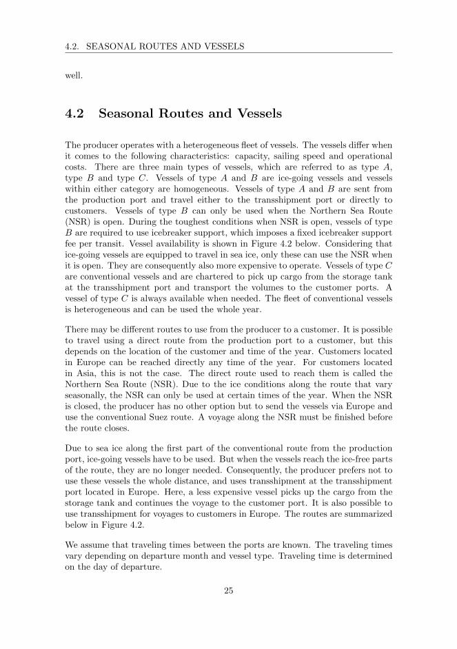
The producer operates with a heterogeneous fleet of vessels. The vessels differ whenit comes to the following characteristics: capacity, sailing speed and operationalcosts. There are three main types of vessels, which are referred to as type A,type B and type C. Vessels of type A and B are ice-going vessels and vesselswithin either category are homogeneous. Vessels of type A and B are sent fromthe production port and travel either to the transshipment port or directly tocustomers. Vessels of type B can only be used when the Northern Sea Route(NSR) is open. During the toughest conditions when NSR is open, vessels of typeB are required to use icebreaker support, which imposes a fixed icebreaker supportfee per transit. Vessel availability is shown in Figure 4.2 below. Considering thatice-going vessels are equipped to travel in sea ice, only these can use the NSR whenit is open. They are consequently also more expensive to operate. Vessels of type Care conventional vessels and are chartered to pick up cargo from the storage tankat the transshipment port and transport the volumes to the customer ports. Avessel of type C is always available when needed. The fleet of conventional vesselsis heterogeneous and can be used the whole year.
There may be different routes to use from the producer to a customer. It is possibleto travel using a direct route from the production port to a customer, but thisdepends on the location of the customer and time of the year. Customers locatedin Europe can be reached directly any time of the year. For customers locatedin Asia, this is not the case. The direct route used to reach them is called theNorthern Sea Route (NSR). Due to the ice conditions along the route that varyseasonally, the NSR can only be used at certain times of the year. When the NSRis closed, the producer has no other option but to send the vessels via Europe anduse the conventional Suez route. A voyage along the NSR must be finished beforethe route closes.
Due to sea ice along the first part of the conventional route from the productionport, ice-going vessels have to be used. But when the vessels reach the ice-free partsof the route, they are no longer needed. Consequently, the producer prefers not touse these vessels the whole distance, and uses transshipment at the transshipmentport located in Europe. Here, a less expensive vessel picks up the cargo from thestorage tank and continues the voyage to the customer port. It is also possible touse transshipment for voyages to customers in Europe. The routes are summarizedbelow in Figure 4.2.
We assume that traveling times between the ports are known. The traveling timesvary depending on departure month and vessel type. Traveling time is determinedon the day of departure.
25

CHAPTER 4. PROBLEM DESCRIPTION
Figure 4.2: The figure shows the different routes from the producer’s port, and whichvessels that may use which route.
4.3 LNG Cargo and Partial Loading
4.3.1 Boil-off
When an LNG vessel has embarked on a voyage, the cargo is reduced daily with afixed natural boil-off rate. This means that the amount of cargo picked up differsfrom the amount of cargo unloaded at a port. For vessels of type A and B, bothnatural and forced boil-off occur. The latter is a fixed amount of LNG from thetanks that is purposely ”forced” to use as fuel. Since the vessels are in dock duringloading and unloading processes, the forced boil-off amount is lower than duringsailing. Cargo transported by vessels of type C are only subject to a fixed dailynatural boil-off rate.
4.3.2 Partial Loading
The LNG volume loaded onto a vessel at the production port depends on whetherthe vessel is headed to the transshipment port or directly to a customer.
The common industry practice is to operate with full ship loads. However, due toquite limited storage space in the tank at the transshipment port, some residualmight be left after loading and unloading operations. The residual amount mightbecome big enough to prevent a vessel from unloading a full ship load and creates abottleneck. Instead of unloading the ship load partially at the transshipment portand travel back to the production port with partial loads, an alternative approachcould be to load the vessels partially at the production port. In this case, theproducer may load the vessel with a volume that is just enough to fully unloadthe cargo at the transshipment port. This is called partial loading. Partial loading
26

4.3. LNG CARGO AND PARTIAL LOADING
would operate with the same amount of LNG as for partial deliveries. Since thestorage tank at the transshipment port is only operated by the LNG producer, weassume that the producer is aware of the inventory level during the whole planninghorizon. In order to prevent sloshing, the loading volume should be at least γpercent of the vessel’s total tank volume.
Partial loading only applies to the voyages between the production and transship-ment ports. Voyages directly to customers or spot markets deal with full shiploadsonly.
27

CHAPTER 4. PROBLEM DESCRIPTION
28
Chapter 5
Mathematical Model
In this chapter, we formulate the ADP planning problem as a mixed integer pro-gramming (MIP) model. The mathematical model presented here is based on themodel in Bugge and Thavarajan (2017), but some changes are made. A majorchange is the implementation of partial loading.
5.1 Assumptions
The following assumptions and simplifications are made in order to reduce thecomplexity of the problem. Some of these assumptions and simplifications are alsopresented in Bugge and Thavarajan (2017).
• The duration of a one-way trip, Tijvt is assumed to be integer. Tijvt includesthe day when cargo is loaded onto the vessel at the loading port and 2Tijvtincludes both the loading day and the day when the cargo is unloaded at thetransshipment port or at a customer.
• There are four types of conventional vessels, with a given number of eachtype. However, the total amount of all the conventional vessels are assumedto be non-limiting, and there is at least one conventional vessel available topick up cargo at the transshipment port.
• During a day, only one operation is possible. This implies that on a givenday, a vessel is either sailing, loading cargo, unloading cargo or idle.
29

CHAPTER 5. MATHEMATICAL MODEL
5.2 Notation
Indices
i, j Origin and destination point.
m Time interval.
v Vessel.
t Time period.
Sets
C Set of customers.
CA Set of customers, both long-term and spot, that cannot be visiteddirectly, when the NSR is closed, CA ⊂ C.
CD Set of customers, both long-term and spot, that can be visiteddirectly or via transshipment, CD ⊂ C.
CLT Set of customers with long-term contracts. It is mandatory toserve these customers, CLT ⊂ C.
CS Set of spot markets. CS ⊂ C.M Set of time intervals.
P Set of ports.
PO Set of producer ports, PO ⊂ P.
PT Set of transshipment ports, PT ⊂ P.
V Set of vessels.
VA Set of vessels of type A, VA ⊆ V.
VB Set of vessels of type B, VB ⊆ V.
VC Set of conventional vessels, VC ⊆ V.
T Set of time periods.
T Set of time periods used for the parameter describing when theNorthern Sea Route is open.
T ijvt Set of departure times where the arrival time is outside theplanning horizon, that is t ∈ T ijvt if t + Tijvt >| T | andt ∈ T , T ijvt ⊂ T .
Tm Set of time periods in time interval m, Tm ⊂ T .
Note that the set of customers, C, can be divided into two subsets based on customertype, CLT , CS . The set of ports P, can be divided into the subsets PO and PT .
30

5.2. NOTATION
Parameters
Bi Number of berths available at port i.
Cijvt Shipping costs for vessel v embarking on a round trip from i to jat time t.
C+j Annual penalty cost for over-delivery below one shipload at cus-
tomer j.
C−j Annual penalty cost for under-delivery below one shipload at cus-tomer j.
C+
j Annual penalty cost for over-delivery above one shipload at cus-tomer j.
C−j Annual penalty cost for under-delivery above one shipload at cus-
tomer j.
C+jm Penalty cost for over-delivery at customer j in time interval m.
C−jm Penalty cost for under-delivery at customer j in time interval m.
Djm Total demand at customer j during the time interval m.
FL Forced boil-off when loading or unloading.
FS Forced boil-off when sailing.
Nvt An indicator parameter. Is equal to 1 if the Northern Sea Routeis open at time t for vessel type v, 0 otherwise. t ∈ T .
O Remaining percentage of cargo in vessel v due to natural boil-off.O = 1− daily boil-off rate .
Pt LNG production rate at the producer during time t.
RSjt Revenue from selling a unit of LNG in the spot market located atcustomer j at time t.
Si Upper storage limit at port i.
Si Lower storage limit at port i.
si0 Initial storage level at port i.
Tijvt Travel time from i to j using vessel v. The travel time includesloading time t at port i and depends on t. Unloading at port jis not included in Tijvt. 2Tijvt describes the total travel time forthe round trip.
Qj Lowest possible cargo delivered to customer j.
Qv Amount of cargo collected by vessel v.
Qijvt Cargo transported from port i and delivered at customer j, byvessel v. The cargo is picked up by vessel v at time t.
αijvt Parameter used for calculating cargo delivered to port PT fromPO.
31

CHAPTER 5. MATHEMATICAL MODEL
βijvt Parameter used for calculating cargo delivered to port PT fromPO.
γ Parameter used for calculating lower bound on cargo picked upwhen sailing from port PO to PT . In order to avoid sloshing, γ isset equal to 0.7
Decision Variables
a+j Total over-delivery to customer j ∈ CLT above one ship load, forthe whole planning horizon.
a−j Total under-delivery to customer j ∈ CLT above one shipload, forthe whole planning horizon.
lijvt Cargo picked up when sailing from i ∈ PO to j ∈ PT at timet ∈ T for vessel v ∈ VA ∪ VB .
sit Storage level at port i ∈ P at the end of time period t.
xijvt Is 1 if vessel v picks up cargo at port i ∈ PO ∪ PT the followingday, at time t ∈ T and travels to j ∈ PT ∪ C, 0 otherwise. Notethat i 6= j.
y+j Total over-delivery to customer j ∈ CLT below one shipload, forthe whole planning horizon.
y−j Total under-delivery to customer j ∈ CLT below one shipload, forthe whole planning horizon.
y+jm Over-delivery to customer j ∈ CLT in time interval m ∈M.
y−jm Under-delivery to customer j ∈ CLT in time interval m ∈M.
zijvt Cargo unloaded at port j ∈ PT at time t ∈ T , when travelingfrom i ∈ PO with vessel v ∈ VA ∪ VB .
5.3 Model Description
Objective
min∑
i∈PO∪PT
∑j∈{C∪PT |j 6=i}
∑v∈V
∑t∈T
Cijvtxijvt +∑j∈CLT
(C+
j a+j + C
−j a−j )
+∑j∈CLT
(C+j y
+j + C−j y
−j ) +
∑j∈CLT
∑m∈M
(C+jmy
+jm + C−jmy
−jm)
−∑
i∈PO∪PT
∑j∈CS
∑v∈V
|T |−Tijvt∑t=1
RSjtQijvtxijvt
(5.1)
32

5.3. MODEL DESCRIPTION
The objective function (5.1), aims to minimize the costs related to fulfilling thelong term contracts. It consist of costs related to transportation, penalty due toover- and under-delivery, and sales in spot markets. Over- and under-delivery existboth on monthly and annual basis, while sales in the spot market are consideredas negative costs. Operative costs related to sailing are considered in the firstterm in the objective. The second and the third term describes the cost related toover- and under-delivery on an annual basis. The second terms provides a positivecontribution to the objective value if total over- or under-delivery exceeds one shipload, while the third term provides costs if they are lower. Monthly over- andunder-delivery is included in the fourth term, while revenue from sales in spotmarkets are considered in the fifth term.
Routing Constraints
∑i∈PO∪PT
∑j∈{C∪PT |j 6=i}
∑{τ∈T |max(1, t−2Tijvτ+1)≤τ≤t}
xijvτ ≤ 1 v ∈ V, t ∈ T
(5.2)
Constraints (5.2) make sure that each vessel returns before making a new trip.Note that the traveling time for one vessel to a given customer is dependent onloading day, and vary throughout the planning horizon.
∑j∈C∪PT
∑v∈V
xijvt ≤ Bi, i ∈ PO, t ∈ T (5.3)
∑i∈PO
∑v∈VA∪VB
∑{τ∈T |τ+Tijvτ=t}
xijvτ +∑i∈C
∑v∈VC
xjivt ≤ Bj , j ∈ PT , t ∈ T
(5.4)
Constraints (5.3) and (5.4) ensure that the number of vessels loading or unloadingat the origin and transshipment port not exceeds the berth capacity at the port. Atorigin, the berth capacity concerns vessels loading cargo, while the berth capacityat the transshipment port deals with both loading and unloading.
2Tijvtxijvt ≤∑
t≤τ<t+2Tijvt
Nvτ , i ∈ PO, j ∈ CA, v ∈ VA, t ∈ T (5.5)
When the Northern Sea Route is open, vessels of type A may travel directly tocustomers located in Asia, if the route is open during the whole voyage. Thisis handled in constraints (5.5). Note that the summation of τ may exceed theplanning horizon.
33

CHAPTER 5. MATHEMATICAL MODEL
2Tijvtxijvt ≤∑
t≤τ<t+2Tijvt
Nvτ , i ∈ PO, j ∈ C ∪ PT , v ∈ VB , t ∈ T (5.6)
Vessel B cannot be used at all when the Northern Sea Route is closed. Thus,constraints (5.6) make sure that vessels of type B can only be used when the routeis open. Note that the summation of τ may exceed the planning horizon.
Demand Fulfillment Constraints
∑i∈PO∪PT
∑v∈V
∑{t∈T |t+Tijvt∈Tm}
Qijvtxijvt + y−jm − y+jm = Djm, j ∈ CLT , m ∈M
(5.7)∑i∈PO∪PT
∑v∈V
∑t∈T
Qijvtxijvt + y−j + a−j − y+j − a
+j =
∑m∈M
Djm, j ∈ CLT (5.8)
Demand fulfillment is handled in constraints (5.7) and (5.8). The periodical de-mand is handled for each time interval in constraints (5.7) while the total demandis handled in (5.8). The constraints are formulated as soft constraints, which allowsover- and under-deliveries.
y−j ≤ Qj , j ∈ CLT (5.9)
y+j ≤ Qj , j ∈ CLT (5.10)
Constraints (5.9) and (5.10) ensure that the y−j and y−j are below one shipload,
and that a+j and a−j are above.
Inventory Constraints
sit−si(t−1) +∑j∈C
∑v∈VA∪VB
Qvxijvt+∑j∈PT
∑v∈VA∪VB
lijvt−Pt = 0, i ∈ PO, t ∈ T
(5.11)
sjt − sj(t−1) −∑i∈PO
∑v∈VA∪VB
zijvt +∑
i∈CA∪CD
∑v∈VC
Qvxjivt = 0,
j ∈ PT , t ∈ T(5.12)
34

5.3. MODEL DESCRIPTION
Si ≤ sit ≤ Si, i ∈ PO ∪ PT , t ∈ T (5.13)
Constraints (5.11)-(5.13) handle the inventory level at the origin and transshipmentport. Constraints (5.11) describes the inventory level at the origin port as a resultof production rate, cargo picked up and the storage level from the previous timeperiod. The constraints consist of two parts describing cargo picked up, Qvxijvtand lijvt. The first part is cargo picked up for delivery to customers or to the spotmarket. The second, describes cargo picked up for delivery to the transshipmentport. The cargo delivered to the transshipment port is not necessarily a full shipload. Constraints (5.12) handle the inventory level of the storage tank at thetransshipment port. This inventory level is formulated as result of cargo deliveredfrom origin, cargo picked up and the inventory level from the previous time period.
Partial Loading Constraints
zijv(t+Tijvt) = αijvtlijvt−βijvtxijvt, i ∈ PO, j ∈ PT , v ∈ VA∪VB , t ∈ T \T ijvt(5.14)
Constraints (5.14) describe the z-variable as the amount of cargo unloaded at thetransshipment port. t+ Tijvt is the day the unloading process occurs, and the daythe vessel occupies the berth at the port. As a result of boil-off, the z-variableis smaller than the l-variable. The cargo delivered to the transshipment port, isequal to cargo picked up at the origin multiplied with a rate αijvt, minus βijvt.αijvt and βijvt are results of both forced and natural boil-off. The derivation ofαijvt and βijvt is presented in Appendix A, and the expressions are: αijvt = OTijvt
and βijvt = FLOTijvt +FS(OTijvt−1O−1 − 1) +FL + FS
O (( 1O )Tijvt−1−1
1O−1
), where O is the
remaining percentage of cargo in vessel v due to natural boil-off. O = 1− dailyboil-off rate.
lijvt −Qvxijvt ≤ 0, i ∈ PO, j ∈ PT , v ∈ VA ∪ VB , t ∈ T (5.15)
lijvt − γQvxijvt ≥ 0, i ∈ PO, j ∈ PT , v ∈ VA ∪ VB , t ∈ T (5.16)
Constraints (5.15)-(5.16) are big-m and small-m formulations used to connect thecontinuous l-variables with the binary x-variables. (5.15) ensure that if xijvt = 1,lijvt gets a value smaller or equal to Qv. However, constraint (5.16) prevent lijvtfrom being smaller than γQv.
35
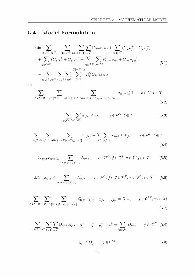
CHAPTER 5. MATHEMATICAL MODEL
5.4 Model Formulation
min∑
i∈PO∪PT
∑j∈{C∪PT |j 6=i}
∑v∈V
∑t∈T
Cijvtxijvt +∑j∈CLT
(C+
j a+j + C
−j a−j )
+∑j∈CLT
(C+j y
+j + C−j y
−j ) +
∑j∈CLT
∑m∈M
(C+jmy
+jm + C−jmy
−jm)
−∑
i∈PO∪PT
∑j∈CS
∑v∈V
|T |−Tijvt∑t=1
RSjtQijvtxijvt
(5.1)
s.t ∑i∈PO∪PT
∑j∈{C∪PT |j 6=i}
∑{τ∈T |max(1, t−2Tijvτ+1)≤τ≤t}
xijvτ ≤ 1 v ∈ V, t ∈ T
(5.2)
∑j∈C∪PT
∑v∈V
xijvt ≤ Bi, i ∈ PO, t ∈ T (5.3)
∑i∈PO
∑v∈VA∪VB
∑{τ∈T |τ+Tijvτ=t}
xijvτ +∑i∈C
∑v∈VC
xjivt ≤ Bj , j ∈ PT , t ∈ T
(5.4)
2Tijvtxijvt ≤∑
t≤τ<t+2Tijvt
Nvτ , i ∈ PO, j ∈ CA, v ∈ VA, t ∈ T (5.5)
2Tijvtxijvt ≤∑
t≤τ<t+2Tijvt
Nvτ , i ∈ PO, j ∈ C ∪ PT , v ∈ VB , t ∈ T (5.6)
∑i∈PO∪PT
∑v∈V
∑{t∈T |t+Tijvt∈Tm}
Qijvtxijvt + y−jm − y+jm = Djm, j ∈ CLT , m ∈M
(5.7)
∑i∈PO∪PT
∑v∈V
∑t∈T
Qijvtxijvt + y−j + a−j − y+j − a
+j =
∑m∈M
Djm, j ∈ CLT (5.8)
y−j ≤ Qj , j ∈ CLT (5.9)
36

5.4. MODEL FORMULATION
y+j ≤ Qj , j ∈ CLT (5.10)
sit−si(t−1) +∑j∈C
∑v∈VA∪VB
Qvxijvt+∑j∈PT
∑v∈VA∪VB
lijvt−Pt = 0, i ∈ PO, t ∈ T
(5.11)
sjt − sj(t−1) −∑i∈PO
∑v∈VA∪VB
zijvt +∑
i∈CA∪CD
∑v∈VC
Qvxjivt = 0,
j ∈ PT , t ∈ T(5.12)
Si ≤ sit ≤ Si, i ∈ PO ∪ PT , t ∈ T (5.13)
zijv(t+Tijvt) = αijvtlijvt−βijvtxijvt, i ∈ PO, j ∈ PT , v ∈ VA∪VB , t ∈ T \T ijvt(5.14)
lijvt −Qvxijvt ≤ 0, i ∈ PO, j ∈ PT , v ∈ VA ∪ VB , t ∈ T (5.15)
lijvt − γQvxijvt ≥ 0, i ∈ PO, j ∈ PT , v ∈ VA ∪ VB , t ∈ T (5.16)
xijvt ∈ {0, 1}, i ∈ PO, j ∈ C ∪ PT , v ∈ V, t ∈ T (5.17)
y+j , y−j , a+j , a−j ≥ 0, j ∈ CLT (5.18)
y+jm, y−jm ≥ 0, j ∈ CLT , m ∈M (5.19)
lijvt, zijvt ≥ 0, i ∈ PO, j ∈ PT , v ∈ VA ∪ VB , t ∈ T (5.20)
37

CHAPTER 5. MATHEMATICAL MODEL
38

Chapter 6
Solution Methods
In this chapter, we present two solution methods to solve the ADP planning prob-lem. A rolling horizon heuristic (RHH) is described Section 6.1, while an aggrega-tion and disaggregation heuristic (ADH) that solves a reduced instance of the fullproblem is discussed in Section 6.2.
6.1 Rolling Horizon Heuristic
The goal of the planning problem in this thesis is to create a cost effective ADP forthe LNG-producer over a long time horizon. The length of the time horizon itself isa challenge when it comes to computational efficiency. As discussed in Chapter 3,rolling horizon methods can be applied to scheduling problems in order to producegood solutions within reasonable time. The heuristic solves the ADP planningproblem in sub-horizons, which means that we solve smaller problems iteratively.RHH as a solution method provided good solutions for the ADP planning problemstudied by Rakke et al. (2011), which motivates us to use the same approach.
Description
The idea behind RHH is to divide the planning horizon into shorter sub-horizonsand solve the ADP planning problem through a series of iterations. In each iter-ation, the MIP is solved for one sub-horizon. Since the complexity of solving theproblem is reduced by considering one sub-horizon at a time, the overall compu-tational time may be improved. When the heuristic terminates, a feasible solutionto the ADP planning problem for the whole planning horizon is returned, whichconsists of the solutions from solving each sub-horizon.
When solving the ADP planning problem, we divide the planning horizon into sub-
39
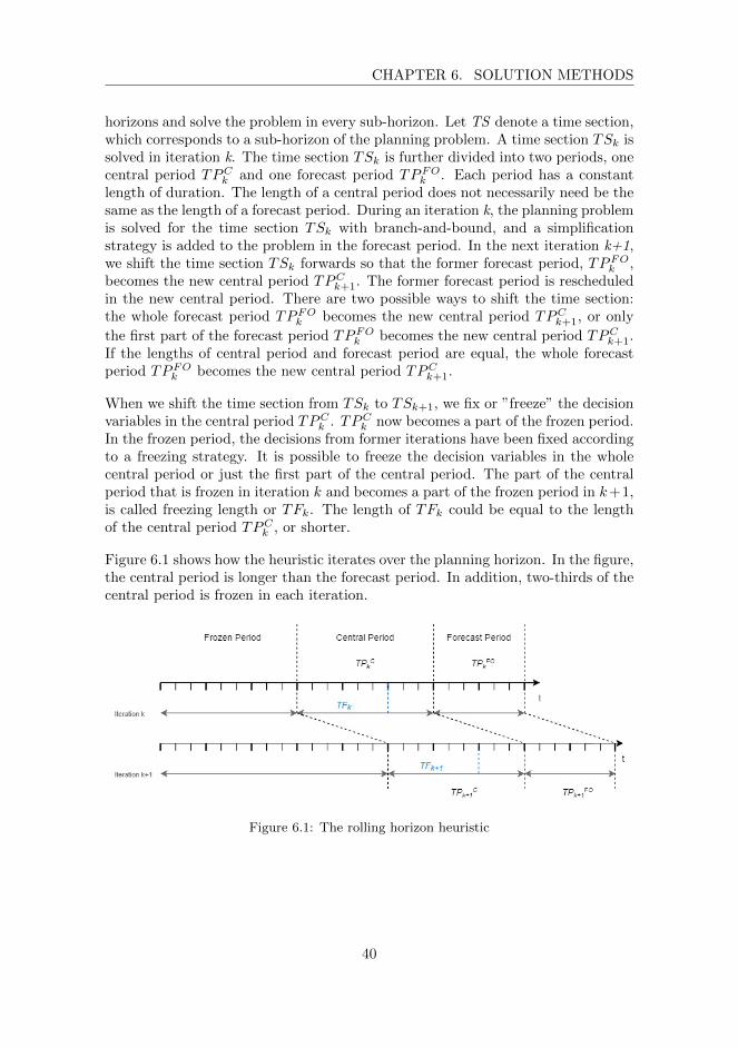
CHAPTER 6. SOLUTION METHODS
horizons and solve the problem in every sub-horizon. Let TS denote a time section,which corresponds to a sub-horizon of the planning problem. A time section TSk issolved in iteration k. The time section TSk is further divided into two periods, onecentral period TPCk and one forecast period TPFOk . Each period has a constantlength of duration. The length of a central period does not necessarily need be thesame as the length of a forecast period. During an iteration k, the planning problemis solved for the time section TSk with branch-and-bound, and a simplificationstrategy is added to the problem in the forecast period. In the next iteration k+1,we shift the time section TSk forwards so that the former forecast period, TPFOk ,becomes the new central period TPCk+1. The former forecast period is rescheduledin the new central period. There are two possible ways to shift the time section:the whole forecast period TPFOk becomes the new central period TPCk+1, or only
the first part of the forecast period TPFOk becomes the new central period TPCk+1.If the lengths of central period and forecast period are equal, the whole forecastperiod TPFOk becomes the new central period TPCk+1.
When we shift the time section from TSk to TSk+1, we fix or ”freeze” the decisionvariables in the central period TPCk . TPCk now becomes a part of the frozen period.In the frozen period, the decisions from former iterations have been fixed accordingto a freezing strategy. It is possible to freeze the decision variables in the wholecentral period or just the first part of the central period. The part of the centralperiod that is frozen in iteration k and becomes a part of the frozen period in k+1,is called freezing length or TFk. The length of TFk could be equal to the lengthof the central period TPCk , or shorter.
Figure 6.1 shows how the heuristic iterates over the planning horizon. In the figure,the central period is longer than the forecast period. In addition, two-thirds of thecentral period is frozen in each iteration.
Figure 6.1: The rolling horizon heuristic
40

6.1. ROLLING HORIZON HEURISTIC
The Central Period
For each central period, we update the accumulated deviation in deliveries. Theaccumulated deviation in deliveries describe the total over- or under-delivery deliv-ered to a customer during a period of time. In each central period, the accumulateddeviation is equal to the sum of monthly deviations from the previous iterationsand deviations in the current central period. At the end of the planning horizon,the accumulated deviation for a customer will be equal to the annual demand lessthe amount of cargo delivered in the whole planning horizon.
We update the accumulated deviations by calculating the difference in demandand cargo delivered, for all previous and the current central period. If we let T CPdenote the set of time periods in the central period,MCP the set of time intervalsin the central period, T F the set of time intervals in the frozen period, and letMF
be the set of time intervals in the frozen period, the annual demand-constraints(5.8) can be reformulated as:∑
i∈PO∪PT
∑v∈V
∑{t∈T |t+Tijvt∈T CP }
Qijvtxijvt + y−j + a−j − y+j − a
+j =
∑m∈MF∪MCP
Djm −∑
i∈PO∪PT
∑v∈V
∑{t∈T F |t+Tijvt∈T F }
Qijvtxijvt, j ∈ CLT
Where y−j , a−j , y+j , a+j is used to describe the accumulated deviation in deliveriesfor one customer.
The Frozen Period
The decision variables from the central period are frozen according to a freezingstrategy before proceeding to the next iteration. There are two relevant freezingstrategies to consider: we either freeze all of the decision variables or only thebinary decision variables from the central period. The first option reduces thesolution space for the next iteration considerably, since vessels are fixed to a voy-age and cannot be used again before return time. This also prevents the modelfrom changing the loading volumes for transshipment and storage values in lateriterations.
The Forecast Period
In the forecast period, a simplification strategy is applied to the problem. Thereare two things to consider when designing the forecasting period. The first is thesimplification strategy, while the second concerns the length.
When we select a simplification strategy, we determine whether to relax the binary
41

CHAPTER 6. SOLUTION METHODS
restrictions on the decision variables in the forecast period or not. According toRakke et al. (2011), when the decision variables take on continuous values, we riskless accurate forecasting information for the next periods. But in return, we mightreduce some computational effort during the solution process. When it comes tothe length of the forecast period, Rakke et al. (2011) argue that the forecast lengthshould be long enough to be affected by and affect decisions made in the centralperiod. It is worth mentioning that the length of the forecast period also affectsthe size of the problem we solve in each iteration. Therefore, in order to reducethe computational time, the forecast period should be rather short. At the sametime, if a voyage has a departure day during the central period and a return dayafter the end of the central period, the forecast period should be long enough toinclude the return day.
Transfer of Information
At the end of each iteration, some information is transferred to the next iteration.When the accumulated deviations are updated in each iteration, the departures inthe frozen period must be known.
In addition to accumulated deviations, other information should be transferredbetween the iterations. The storage level on the last day in TFk becomes the theinitial storage level in the central period TPCk+1 and should therefore be transferred.In iteration k+ 1 the model should also be aware of departed vessels that have notreturned by the end of the previous central period TPCk . These decisions affect thevessel availability in iteration k + 1 and should thus be included in the iteration.
6.2 Aggregation and Disaggregation Heuristic
In the previous section, RHH is proposed as an approach to solve the ADP planningproblem by solving a reduced version of the problem iteratively. Another approachto reduce the size of the problem is to aggregate the nodes in a problem and solvethe reduced case. The solution to the reduced problem is then disaggregated. Wedevelop an Aggregation and Disaggregation Heuristic (ADH) for this purpose.
The ADH consists of two components: the aggregation of nodes in a probleminstance and disaggregation of a solution to the reduced problem instance. Theprocedure is shown below in Figure 6.2. Customers, or nodes, are clustered to-gether and becomes an aggregated customer. The aggregation of nodes is basedon the geographic area of the customers. The aggregated problem instance is thensolved with branch-and-bound to get a set of feasible solutions. The solutions arethen given as input to a Disaggregation Heuristic (DH), which disaggregates the so-lution by rerouting the voyages to aggregated nodes to individual customers. With
42

6.2. AGGREGATION AND DISAGGREGATION HEURISTIC
exact methods, the computational time increase exponentially when the number ofnodes increase. A reduction of the number of nodes in the network can lead to areduction in the computational time, and consequently produce a delivery schedulein a shorter amount of time (Rogers et al., 1991). The ADH may be used to givethe producer an idea of a potential ADP when the number of buyers increase ordecrease, or when demands are adjusted.
Figure 6.2: Overview of the Aggregation Disaggregation Heuristic
According to Rogers et al. (1991), the nodes should be grouped according to aclustering strategy. The clustering strategies are based on similarities, so thaterror or data loss is minimized during the aggregation and disaggregation process.We choose to cluster the long-term customers located in the same geographic areas:Europe and Asia. If we were to cluster the nodes without having geographic areasin mind, the disaggregated solution would consist of substantial spread in traveltimes. The two aggregated, long-term, customers are denoted as LT-EU and LT-Asia.
Besides the long-term customers, there is one spot customer in each geographicarea. The producer may send a ship load to spot customers when there is excessLNG left in the production tanks, while for the long-term customers, the produceris obligated to send ship loads every month to fulfill the demand stated in thecontracts. Hence, due to differences in delivery purposes, the spot-customers arenot clustered together with the long-term customers.
The next step is to decide how the parameter values of each individual node ishandled during aggregation. The demand of one aggregated customer is equalto the sum of the demands of each individual customer that is “included” in theaggregated customer. The aggregated customers are assigned the longest traveltimes among their individual customers to prevent routing infeasibility when thevessels are rerouted. This way, the vessels are rerouted so that they arrive beforeor at the same time as the solution of the aggregated case. After aggregation, thereduced problem instance is solved with branch-and-bound.
Since we cluster the nodes according to geographic areas, the disaggregation isa straightforward procedure. Voyages scheduled to an aggregated customer arererouted to the individual customers in the same geographic area. Algorithm 1below shows the disaggregation procedure. When the heuristic disaggregates thevoyages in the initial solution, it needs to take berth, inventory and routing feasibil-ity into consideration. For the voyages where partial loading applies, the heuristicdoes not change the value of the cargo picked up.
43

CHAPTER 6. SOLUTION METHODS
Algorithm 1: Disaggregation of Voyages
Initialization:Let Sa be the set of voyages from the initial solution of the aggregated caseS = ∅Let M be the set of months in the planning horizonLet C be the set of customers in the larger casefor m ∈M do
if m = 0 or m = NSR open or m = NSR closed thenSort C based on travel times
endfor s ∈ Sa do
if s goes to spot customer or transshipment port thenS ← S ∪ s
endelse
for c ∈ C doif customer c has unfulfilled demand in month m then
sr ← reroute the voyage to customer cS ← S ∪ srUpdate remaining demand in month m for customer c
endif initial voyage s is not assigned to any customers then
sr ← reroute the voyage to a spot customer in the samegeographic areaS ← S ∪ sr
end
end
end
endCalculate the deviation in month m for all customers
endCalculate annual deviation for all customersCalculate objectivereturn S
6.2.1 Description of Disaggregation Procedure
The heuristic starts with reading the initial solution Sa from the aggregated case.The solution contains planned voyages and departure times to the aggregated cus-tomers, and the heuristic reroutes the voyages and determines the new destinationand new arrival time. Sa is sorted chronologically by departure times. Since eachaggregated customer is assigned the longest travel time from the producer’s or
44

6.2. AGGREGATION AND DISAGGREGATION HEURISTIC
transshipment port, we avoid the issue of new arrival dates ending up in the nextmonth after rerouting, thus missing the demand for the current month.
The algorithm is initiated with an empty set of distributed voyages S. There isalso a set of customers C for each aggregated customer, where these customersare in the same geographical area as the aggregated customer. The customers areprioritized by travel times in decreasing order, so that customers with the longesttravel times are prioritized first. In combination with Sa sorted chronologically,this should prevent the new arrival dates from being set the previous month m-1,if the initial voyage s has departure time in month m-1 and arrival time in monthm.
The algorithm then begins iterating through the list of voyages with arrival timesin month m. If the voyage is headed to an aggregated customer, the heuristicuses the set of customers that are in the same geographic area as the aggregatedcustomer and proceeds to rerouting. If the voyage on the other hand, heads to thetransshipment port or to a spot customer, the voyage is added to the result set Sand the heuristic proceeds to the next voyage.
At the rerouting stage, the heuristic first chooses a customer c from the set ofcustomers C. If the customer has been assigned enough voyages to satisfy themonthly demand, the heuristic proceeds to the next customer in the list. Otherwise,the customer is assigned the voyage. If a voyage cannot be rerouted to any ofthe customers, the voyage is rerouted to a spot customer in the same geographicarea as the corresponding aggregated customer. This is the case if a customer islocated at the transshipment port and cannot be assigned a voyage departing fromthe transshipment port, and the other customers have been assigned their voyages.The following attributes of the rerouted voyage sr need to be updated: destination,travel time, boil-off adjusted amount of cargo delivered, and vessel availability. Themodified voyage sr is then added to the result set S.
When the heuristic finishes the rerouting stage, the customer is assigned the newvoyage with arrival in month m, and the remaining demand for customer c inmonth m is updated. After assigning all the initial voyages with arrival times inmonth m, the heuristic calculates the monthly deviations for each customer.
When all voyages from the initial solutions are rerouted, the objective value of theresult set is calculated.
6.2.2 Discussion
The aggregated customers are assigned pessimistic travel times. After disaggre-gation, the idle time for the vessels may increase due to the spread between thepessimistic travel time and the travel times of the individual customers. Amongthe Asian customers, the differences in travel times are 1 or 2 days. For the Eu-
45

CHAPTER 6. SOLUTION METHODS
ropean customers, the spread is bigger, and depends on whether the voyages aremostly via transshipment or direct. Since one of the European customers has theirdelivery destination at the transshipment port, transshipment is not needed, andconsequently the travel time is shorter. A bigger difference between the traveltimes of the customers in an aggregated node can lead to increased idle time forthe vessels in the ADP. Therefore, the travel times should affect the choice of aggre-gation strategy. Due to the choice of pessimistic travel times, the ADH producesa conservative and feasible ADP.
The pessimistic travel times may also lead to over-deliveries to the individual cus-tomers, as a result of smaller loss in cargo due to boil-off when the travel timesbecome shorter during rerouting.
Post Processing
Another consequence of the pessimistic travel times are the rerouted arrival dates.If the solution of the aggregated problem instance contains voyages with arrivaltimes in the beginning of a month m, the voyage might be rerouted so that the newarrival time ends up in the previous month m-1 because of shorter travel time. Thisleads to an under delivery in month m and an over delivery the previous monthm-1. Therefore, a possibility could be to postpone the departure of the voyage atleast t days, while ensuring that the new departure day is inventory, berth androuting feasible (the vessel has to finish the new round trip before embarking on alater voyage).
In addition to shorter traveling times, the choice of vessels can lead to a greatamount of under- and over-deliveries to the customers. After all the voyages arererouted, the deliveries to each customer are evaluated. If customers are sufferingfrom huge over-or under-deliveries, it may be possible to change the destinationfor some of the voyages in order to adjust the amount of cargo delivered. Twovessels that arrive two different customers in the same month are allowed to switchdestinations. We call this a swap. The customers must be a part of the sameaggregated customer, to guarantee that the swap is feasible. In addition, as wewant to improve the solution, the new arrival dates should be within the originalarrival month.
46

Chapter 7
Input Data
This chapter presents an overview of the input data used in the model. Parts of thedata in this chapter are similar to the data described in (Bugge and Thavarajan,2017). For the sake of completeness, a summary of the data is also presentedhere. Problem specific information is not included in this chapter due to non-disclosure agreements. Storage capacities at the producer and transshipment portand characteristics for vessel A and B are therefore not specified in this chapter.Most of the data related to the commodity can be given in m3, tonnes or MMBtu.A table with the conversion rates is shown below in Table 7.1. The data listed inthe table are based on a conversion table in GIIGNL (2018).
Table 7.1: Conversion between units
m3 LNG (liquid) tonnes LNG MMBtu
m3 LNG (liquid) - 0.45 23.12
tonnes LNG 2.21 - 51.02
MMBtu 0.0433 0.0196 -
7.1 Ports
Table 7.2 shows an overview of the ports considered in the problem. The locationsof the customers are chosen based on descriptions in Section 2.1.2, and do notnecessarily reflect the real-life situation. Three types of ports are listed in the table:Production, Transshipment and Customer. The customers are further divided intolong-term and spot customers.
47

CHAPTER 7. INPUT DATA
Table 7.2: Overview of ports and customers considered in the problem. LT denotes thelong-term customer, and S is the spot customers.
Name Customer Type Area
Production - -
Transshipment - Europe
Customer 1 LT Europe
Customer 2 LT Europe
Customer 3 LT Asia
Customer 4 LT Asia
Customer 5 LT Asia
Customer 6 LT Asia
Spot Customer 1 S Europe
Spot Customer 2 S Asia
Production and Transshipment Port
The producer located at the production port yields an annual production of LNG.This annual production is divided into a fixed daily production. There is only oneberth at the production port and the transshipment port.
Long Term Customers
Each of the long-term customers listed in Table 7.2 have a monthly demand thatmust be fulfilled. The customers are located in different parts of the world. Eachcustomer should be visited every month, but the cargo delivered differs from cus-tomer to customer, due to different travel times and boil-off. The sum of themonthly demand for all customers during a year is approximately 90% of the an-nual production.
Spot Customers
Table 7.2 includes two spot customers; one in Europe and one in Asia. Sales tothe spot customers are included as revenue in the planning of the ADP. In 2016,the average spot price in Asia was $5.52/MMBtu (International Gas Union, 2017).The revenue from spot sales to the Asian spot customer is based on average spotprice in Asia and set to be equal to $128 per m3.
Recall from Section 2.1, that the amount of LNG imported to Europe are signifi-
48

7.2. VESSELS
cantly lower than the Asian imports. Based on this, we assume that the revenuefrom spot sales in Europe is smaller compared to the same amount sold in the Asianmarket. It should therefore be preferable to sell the spot cargo in the Asian marketinstead of the European. However, if some of the spot cargoes depart near the endof the planning horizon, it may not be possible to reach the Asian market withinthe planning horizon. In these cases, the LNG should be sold in the Europeanmarket. In 2016, the UK spot price hit a low of $ 3.67/MMBtu (International GasUnion, 2017). Based on this, the revenue from spot sales in Europe is set equal to50 % of the Asian spot price.
7.2 Vessels
The fleet in this problem consists of 41 LNG carriers. The vessels within classifica-tion A and within classification B share the same characteristics, while the vesselsof type C are heterogeneous. Four set of different characteristics are created forvessel C.
LNG carriers do usually have a maximum speed of 21 knots in open water (GIIGNL,2009), and therefore the selected speed range for vessels of type C lies between 15and 20 knots. The selected capacities for the vessels of type C attempt to reflectthe variations in the world LNG tanker fleet, and varies between 135,000 to 161,000m3. The selected capacities are similar to capacities listed in the comprehensiveoverview of the total LNG carrier fleet of 2017, by GIIGNL (2018).
7.2.1 Traveling Time
The traveling time between the ports is calculated for each type of the vessels.When the traveling time is calculated, vessel speed, sea ice level, and distance aretaken into consideration.
The distance between the ports is generated using a tool provided by Marine Traffic(2018). The tool suggests different routes between two ports, where the path withthe shortest distance is chosen. For the voyages between the transshipment portand the Asian customers, the vessels travel through the Suez Canal.
One of the vessel characteristics affecting the traveling time is the vessels’ abilityto travel in harsh sea conditions. Recall from Chapter 4, that only vessels of typeA and B can travel from the producer and that type B is only usable when NSRis open. Due to the distinctive vessel characteristics for the types, the openingmonths for NSR are different for vessels A and B. Vessels of type A can use theroute eastwards from July to November, while type B can use the route from Julyto October. The opening periods are determined based on the Admittance Criteria
49

CHAPTER 7. INPUT DATA
for Navigation stated at the websites of Centre for High North Logistics (CHNL)(CHNL, 2018c).
To evaluate the travel conditions along NSR the Sea Ice Index Animation Tool atthe websites of the National Snow and Ice Data Center is used. The tool showsa graphical image of the median ice edge on a monthly basis from 1978 to 2017,as well as the median ice edge calculated from 1981 to 2010 (National Snow &Ice Data Center, 2018). The graphical image indicates the extent of the ice cover.These areas may require lower speed which influences the traveling time.
7.2.2 Operative Costs
The operative costs differ between the types of vessels. The operative costs we areinterested in can be divided into crew costs, charter cost, canal cost and the costof icebreaker support. The costs are summarized in Table 7.3.
Table 7.3: Operative Costs
Vessel Type Cost Type Cost($)
A & B Crew costs 9,222 per day
B Icebreaker support229,561 or
459,140 per round trip
C Charter costs 55,000-60,000 per day
C Canal costs 350,000 per round trip
For vessels of type A and B crew cost are considered. The crew cost is based onan example given in Lopac (2008). In addition to crew cost, the cost of icebreakersupport is included in the operative costs for vessel B.
When NRS is open, vessel B can use the route. The ice-conditions may vary duringthe opening season, and when the ice-conditions are at the toughest, the vesselsneed icebreaker support. The cost for one transit through the NSR is determinedby the number of navigation zones a vessel pass through, the vessel’s ice class andgross tonnage (CHNL, 2018a). Gross tonnage is a measure of a ships total interiorvolume (Dinsmore, 2011). The cost of icebreaker support is chosen based on a costestimation at the websites of the Centre for High North Logistics (CHNL, 2018b).When the vessels are traveling westwards in July, the fee is estimated to $229,140per round trip, while the cost is estimated to $459,140 per round trip eastwards inJuly and both ways in October.
50

7.2. VESSELS
For the vessels of type C, we only consider a daily charter cost and canal costs. Weassume that the charter cost includes all the operative costs except canal cost. Thecharter cost for vessels of type C is based on an example given in Lopac (2008), andvary in the range between $55,000-$60,000. The canal costs are estimated based onthe vessel type, cargo transported and loading condition (Suez Canal Authority,2017a). A toll calculator is available on the web pages of Suez Canal Authority.Using this calculator, the canal fee is estimated to be $350,000 for a round trip forall the vessels of type C (Suez Canal Authority, 2017b).
Fuel costs are not considered for any of the types of vessels, as we assume vesselA and B use forced boil-off as fuel. For vessel C, we assume that fuel costs areincluded in the charter costs.
7.2.3 Boil-off
The cargo delivered to the customers must be adjusted for boil-off. Here, wedistinguish between natural boil-off and forced boil-off. Natural boil-off is theLNG that vaporizes due to the heat exchange from the soundings, while forcedboil-off implies that some additional LNG are forced into vaporization and used asfuel.
When the conventional vessels depart from the transshipment port, they are fullyloaded. Recall from the previous section that charter costs are assumed to includefuel costs, and we assume that the conventional vessels do not use LNG as fuel.Thus, the reduction of cargo on board these vessels is reduced daily by a fixed ratecaused by natural boil-off. The daily boil-off rate is set to be 0.11%. As mentionedin Chapter 2.2, some LNG should be left in the vessel after delivery, to preservethe temperature in the tank. We assume that the difference in cargo picked upand cargo delivered, is equal to the total amount of natural boil-off for the wholeround trip. Cargo delivered to the customers has been pre-processed beforehandusing the boil-off function shown below.
For the conventional vessels, the boil-off function is given as:
ft = Of(t−1)
Where ft describes the amount of LNG in the vessels on day t, and O = 1−0.0011.
We assume that vessels of type A and B are using forced boil-off as the only typeof fuel. In addition to forced boil-off, the cargo is reduced due to natural boil-off.The daily fuel consumption must be known in order to calculate the amount ofcargo removed as forced boil-off.
To determine the fuel consumption for the vessels, we evaluate the daily fuel con-sumption for a conventional LNG vessel with a capacity of 138 000 m3. With a
51

CHAPTER 7. INPUT DATA
travel speed of 19 knots, the daily fuel consumption is 160 tonnes, and when load-ing or unloading the daily use is 3 tonnes (Lopac, 2008). Vessels A and B are moreheavily equipped and can travel in harsher sea conditions than the conventionalvessels referred to by Lopac (2008). We thus choose to use a fuel consumptionrate for travel speed that is higher than the one used in (Lopac, 2008). The fuelconsumption for type A and B is assumed to be 250 tonnes when traveling and 3tonnes when loading or unloading.
Dodds (2014) presents a factor called Fuel Oil Equivalent Factor. This factor is theconversion ratio between m3 of LNG and the equivalent mass of fuel oil in tones(Dodds, 2014). In (Dodds, 2014), the factor is used for conventional vessels, butwe assume it to be similar for vessels of type A and B. Based on this factor, theamount of cargo removed each day, due to forced boil-off is 520 m3 when the vesselsare sailing, and 6.25 m3 when the vessels are loading or unloading.
The cargo on board vessels of type A and B is reduced daily due to both naturaland forced boil-off. The natural boil-off reduces the amount of cargo each day bya given rate. Hence, the cargo on board the vessel can be given as a recursivefunction of time, when the vessel is sailing:
ft = O(f(t−1) − FS)
where ft is the current amount of cargo in a vessel on day t, O = 1 − 0.0011 ,and FS is the reduction of cargo due to forced boil-off when sailing, FS = 520 m3.When the vessels are traveling between the supplier and customers, it is possibleto pre-process the amount of cargo delivered to the customers. The expression isgiven below, and the derivation can be found in Appendix A.
Qijv(t+Tijvt) = QvOTijvt−FLOTijvt−FS(
OTijvt − 1
O − 1−1)−FL−F
S
O(( 1O )Tijvt−1 − 1
1O − 1
)
Qijv(t+Tijvt) is the cargo delivered to customer j on day t + Tijvt, t is the loading
day, Tijvt the traveling time and FL is the reduction of cargo due to forced boil-off when the vessel is loading or unloading. FL = 6.25m3. When the vesselsare sailing between the supplier and the transshipment port, it is not possibleto pre-process the amount of cargo delivered, as it depends on cargo picked up.Constraints (5.14) are used instead when the vessels are traveling between originand the transshipment port.
7.3 Penalty Costs
In the problem described in this thesis, two kinds of penalty costs exist. Over-and under-deliveries in each month are penalized, in addition to over- and under-deliveries for the entire time horizon. Recall from Chapter 4 that the producer is
52
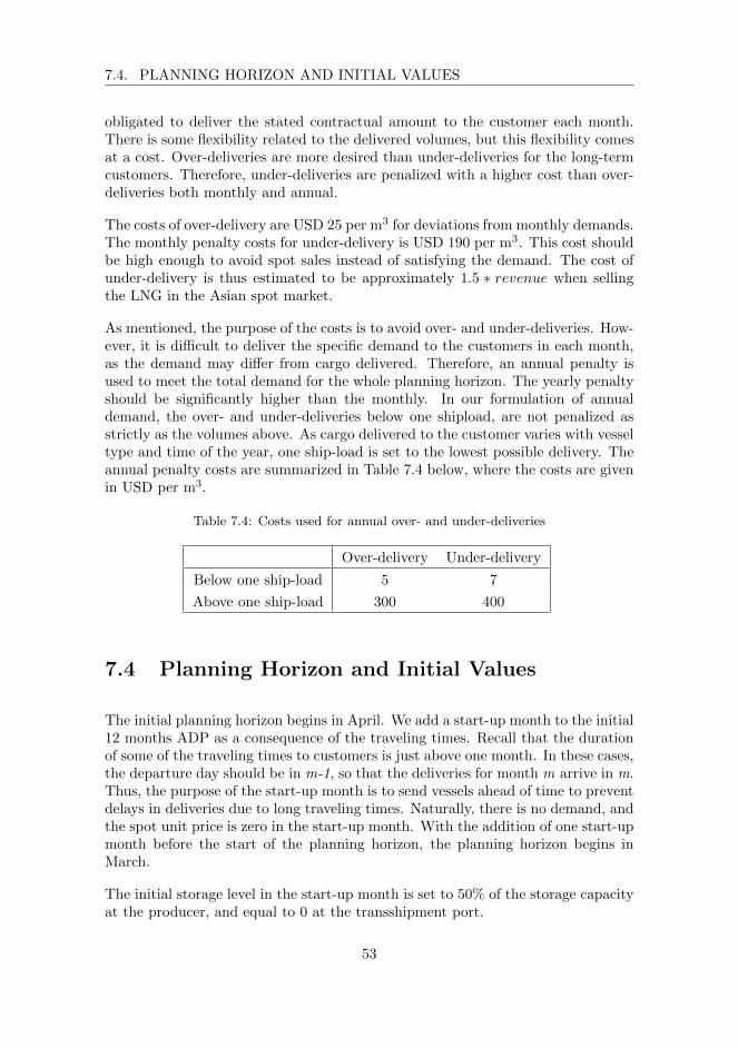
7.4. PLANNING HORIZON AND INITIAL VALUES
obligated to deliver the stated contractual amount to the customer each month.There is some flexibility related to the delivered volumes, but this flexibility comesat a cost. Over-deliveries are more desired than under-deliveries for the long-termcustomers. Therefore, under-deliveries are penalized with a higher cost than over-deliveries both monthly and annual.
The costs of over-delivery are USD 25 per m3 for deviations from monthly demands.The monthly penalty costs for under-delivery is USD 190 per m3. This cost shouldbe high enough to avoid spot sales instead of satisfying the demand. The cost ofunder-delivery is thus estimated to be approximately 1.5 ∗ revenue when sellingthe LNG in the Asian spot market.
As mentioned, the purpose of the costs is to avoid over- and under-deliveries. How-ever, it is difficult to deliver the specific demand to the customers in each month,as the demand may differ from cargo delivered. Therefore, an annual penalty isused to meet the total demand for the whole planning horizon. The yearly penaltyshould be significantly higher than the monthly. In our formulation of annualdemand, the over- and under-deliveries below one shipload, are not penalized asstrictly as the volumes above. As cargo delivered to the customer varies with vesseltype and time of the year, one ship-load is set to the lowest possible delivery. Theannual penalty costs are summarized in Table 7.4 below, where the costs are givenin USD per m3.
Table 7.4: Costs used for annual over- and under-deliveries
Over-delivery Under-delivery
Below one ship-load 5 7
Above one ship-load 300 400
7.4 Planning Horizon and Initial Values
The initial planning horizon begins in April. We add a start-up month to the initial12 months ADP as a consequence of the traveling times. Recall that the durationof some of the traveling times to customers is just above one month. In these cases,the departure day should be in m-1, so that the deliveries for month m arrive in m.Thus, the purpose of the start-up month is to send vessels ahead of time to preventdelays in deliveries due to long traveling times. Naturally, there is no demand, andthe spot unit price is zero in the start-up month. With the addition of one start-upmonth before the start of the planning horizon, the planning horizon begins inMarch.
The initial storage level in the start-up month is set to 50% of the storage capacityat the producer, and equal to 0 at the transshipment port.
53

CHAPTER 7. INPUT DATA
54

Chapter 8
Computational Study
In this chapter, we present the results obtained with the different solutions methods.First, the settings used for the rolling horizon heuristic is determined in Section8.1. Four versions of the heuristic is tested in this section. In Section 8.2 theresults from solving the full case are presented. We solve the full case with anexact solution method in Section 8.2.1 and with the rolling horizon heuristic inSection 8.2.2. In order to create a solution for the full case with the aggregationdisaggregation heuristic (ADH), the aggregated case must be solved. Differentaggregation strategies are discussed and evaluated in Section 8.3.1, before Section8.3.2 presents the results obtained from the heuristic. In Section 8.4 the solutionmethods are compared and evaluated.
For both the exact solution method and RHH, Fico Xpress with Xpress Mosel Ver-sion 4.6.0 and Xpress Optimizer Version 31.01.09 is used. The instances are runon a Elite Desk 800 G2 SFF, with 64-bit Windows 10 Operating System, proces-sor Inter(R) Core(TM) i7-6700 CPU 3.40 GHz and 32.0 GB RAM. The ADH isimplemented in Java version 8.0, with Eclipse Neon as integrated development en-vironment, and run on a Mac OSx environment with 2.6GHz Intel Core i5 processorand 8GB RAM.
8.1 Rolling Horizon Heuristic Settings
In this section, we discuss the different settings for the RHH presented in Chapter6.1. Based on the discussion and results obtained during testing, one strategy ischosen for the heuristic.
When testing the settings, the following stop criteria are set in each iteration:
• Optimality Gap: In each iteration, a limit on the gap between the best so-
55
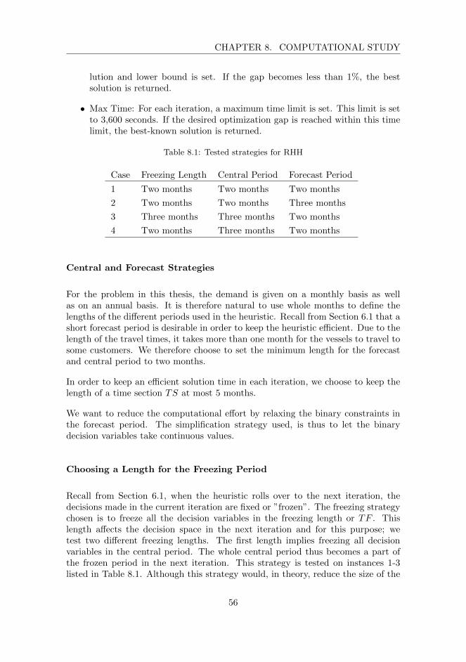
CHAPTER 8. COMPUTATIONAL STUDY
lution and lower bound is set. If the gap becomes less than 1%, the bestsolution is returned.
• Max Time: For each iteration, a maximum time limit is set. This limit is setto 3,600 seconds. If the desired optimization gap is reached within this timelimit, the best-known solution is returned.
Table 8.1: Tested strategies for RHH
Case Freezing Length Central Period Forecast Period
1 Two months Two months Two months
2 Two months Two months Three months
3 Three months Three months Two months
4 Two months Three months Two months
Central and Forecast Strategies
For the problem in this thesis, the demand is given on a monthly basis as wellas on an annual basis. It is therefore natural to use whole months to define thelengths of the different periods used in the heuristic. Recall from Section 6.1 that ashort forecast period is desirable in order to keep the heuristic efficient. Due to thelength of the travel times, it takes more than one month for the vessels to travel tosome customers. We therefore choose to set the minimum length for the forecastand central period to two months.
In order to keep an efficient solution time in each iteration, we choose to keep thelength of a time section TS at most 5 months.
We want to reduce the computational effort by relaxing the binary constraints inthe forecast period. The simplification strategy used, is thus to let the binarydecision variables take continuous values.
Choosing a Length for the Freezing Period
Recall from Section 6.1, when the heuristic rolls over to the next iteration, thedecisions made in the current iteration are fixed or ”frozen”. The freezing strategychosen is to freeze all the decision variables in the freezing length or TF . Thislength affects the decision space in the next iteration and for this purpose; wetest two different freezing lengths. The first length implies freezing all decisionvariables in the central period. The whole central period thus becomes a part ofthe frozen period in the next iteration. This strategy is tested on instances 1-3listed in Table 8.1. Although this strategy would, in theory, reduce the size of the
56

8.1. ROLLING HORIZON HEURISTIC SETTINGS
decision space for the next iteration, problems arise regarding the inventory levelat the transshipment storage tank.
Voyages to the transshipment port with departure times near the end of the centralperiod may cause inconveniences to the inventory level at the port. With a freezinglength equal to the central period, these departures are frozen in the next iterationwhile the corresponding arrival times become parts of the central period. Thestorage capacity is limited at the transshipment port, and since the cargo deliveredto the port may differ from cargo picked up, some departures can become infeasiblewhen the heuristic rolls over the time horizon. Let the following example illustrateone of the problems that may occur at the transshipment port:
Consider iteration k where a vessel departs from the producer at the end of thecentral period, and arrives at the transshipment port on day t in the forecast period.We let the storage level at the transshipment port be at maximum at the start ofthe forecast period. Note that the problem may arise with other storage levels aswell.
If the cargo delivered to the transshipment port on day t is more than the capacityof the vessels picking up cargo at the port, two vessels must depart before the cargocan be delivered on day t. One vessel can depart fully loaded on day t− 2, and theremaining amount of LNG can be removed by another vessel using partial loadingon day t−1. Recall from the previous section that partial loading is allowed in theforecast period due to the simplification strategy.
When the time horizon shifts in iteration k+1, partial loading is no longer allowedon day t − 1, as the day is within the central period. The vessels must be fullyloaded to depart from the transshipment port, and thus the residual amount ofLNG in the tank cannot be removed. Neither is it possible to change the amountof cargo delivered to the port on day t, as the departure corresponding to the arrivaltime on day t is in the frozen period. As a result, the solution obtained in iterationk will become infeasible in iteration k+ 1. Figure 8.1 shows the problem, and howit leads to an infeasible problem in iteration k + 1 when the storage level exceedsmaximum capacity. This is marked with a red line in the figure on the right-handside.
57

CHAPTER 8. COMPUTATIONAL STUDY
Figure 8.1: End of central period-problem at the transshipment port. The left figureshows the inventory level at the transshipment port in iteration k, while the right showsthe inventory level in iteration k + 1.
A possible way to get around this issue is to allow the heuristic to modify theamount of cargo loaded onto vessels traveling between the producer and transship-ment port in the last month of the frozen period. When we test the combinations1-3 listed in Table 8.1, we freeze all the decision variables except for the l-variablesfor the last month in central period. In the next iteration, it is therefore possible tochange the amount of cargo loaded onto the vessels traveling between the producerand transshipment port.
Even though it is possible to modify the cargo picked up at the producer, this maynot be enough to avoid infeasible solutions. We still have strict limits on the l-variables, and the allowed reduction of the variables may not be enough to preventthe infeasible storage level at the transshipment port. Another drawback with theproposed changing of cargo picked up is that a reduction of the l-variable leadsto an increased storage level at the producer. The required modification of cargopicked up may not be possible, as the storage level at the producer can exceedmaximum capacity.
In addition to the infeasibility issues described above, the results obtained from thisstrategy show a tendency towards selecting vessels of type C that are less suitablethan other available vessels on a long-term basis. When the heuristic is planning thedepartures satisfying the demand in the forecast period, some of these departuresare set to central period. In the forecast period, the binary constraints for x-valuesare relaxed. Over- and under-deliveries are thus easily avoided in this period. Inaddition, if a vessel is partially used, the operating costs of using the vessel aremultiplied with the partial x-value. These circumstances make the prioritizing ofvessel of type C different, and vessels that are less suitable on a long-term basismay be chosen.
58

8.2. FULL CASE
The second freezing length tested implies only freezing the first part of the centralperiod in each iteration. The last part of the central period is solved two timeswithout the simplification strategy. This freezing length is tested as case 4 inTable 8.1. When the last month in the central period in iteration k becomes thefirst month in the central period in iteration k+ 1, we avoid the infeasibility issuesdescribed above. It is therefore not necessary to allow changes in the frozen period.This freezing length also avoids the problem related to unsuitable vessels of typeC, as the last month in the central period is rescheduled in the next iteration.
When choosing a strategy, the performance of the tests listed in Table 8.1 areevaluated. Based on the performance we choose to set the forecast period to 2months, and the central period to 3 months. However, in order to avoid end ofcentral period-problems, the freezing length is two months. This strategy providesthe best objective value and lowest deviations from the contractual demands.
With a freezing length of two months, the produced ADP consists of an evennumber of months. Due to the required start-up month described in Section 7.4,we are interested in an ADP consisting of at least 13 months. We thus use seveniterations to create an ADP with a 14-months planning horizon.
8.2 Full Case
In this section, we present the results from solving the full case. The full case consistof the customers listed in Table 7.2 in Section 7.1. The exact solution method ispresented first, before proceeding to the RHH. We consider a 13-months and 14-months planning horizon to create a 12-months ADP as a result of a required start-up month and the choice of RHH-strategies respectively. For the exact method,the case is run until it reaches optimality or a maximum time limit. The maximumtime limit is set to 36,000 seconds.
To evaluate the performance of the RHH, we use the best objective value of theexact method as a lower bound. We therefore present the results of solving theADP planning problem with a 14-months planning horizon by exact method hereas well.
8.2.1 Exact Method
Presolve is a function in Xpress that generates cuts to reduce the number of vari-ables and constraints before the solution process begins. Since the size of the ADPplanning problem affects the computational efficiency, enabling Presolve would re-duce the size of the problem in Xpress by eliminating redundant variables andconstraints early. The size of the problem before and after Presolve is applied, is
59
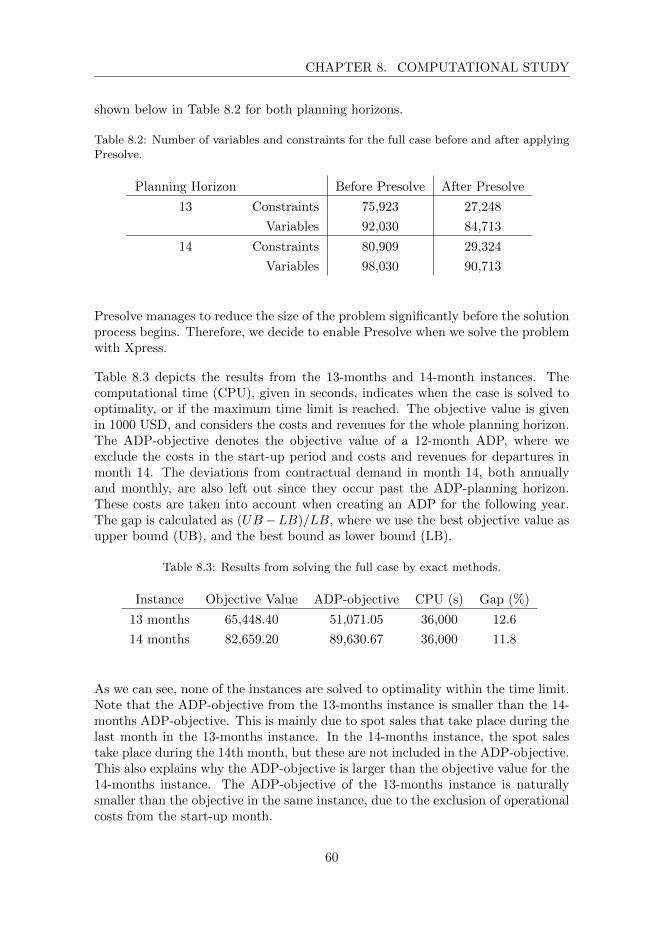
CHAPTER 8. COMPUTATIONAL STUDY
shown below in Table 8.2 for both planning horizons.
Table 8.2: Number of variables and constraints for the full case before and after applyingPresolve.
Planning Horizon Before Presolve After Presolve
13 Constraints 75,923 27,248
Variables 92,030 84,713
14 Constraints 80,909 29,324
Variables 98,030 90,713
Presolve manages to reduce the size of the problem significantly before the solutionprocess begins. Therefore, we decide to enable Presolve when we solve the problemwith Xpress.
Table 8.3 depicts the results from the 13-months and 14-month instances. Thecomputational time (CPU), given in seconds, indicates when the case is solved tooptimality, or if the maximum time limit is reached. The objective value is givenin 1000 USD, and considers the costs and revenues for the whole planning horizon.The ADP-objective denotes the objective value of a 12-month ADP, where weexclude the costs in the start-up period and costs and revenues for departures inmonth 14. The deviations from contractual demand in month 14, both annuallyand monthly, are also left out since they occur past the ADP-planning horizon.These costs are taken into account when creating an ADP for the following year.The gap is calculated as (UB−LB)/LB, where we use the best objective value asupper bound (UB), and the best bound as lower bound (LB).
Table 8.3: Results from solving the full case by exact methods.
Instance Objective Value ADP-objective CPU (s) Gap (%)
13 months 65,448.40 51,071.05 36,000 12.6
14 months 82,659.20 89,630.67 36,000 11.8
As we can see, none of the instances are solved to optimality within the time limit.Note that the ADP-objective from the 13-months instance is smaller than the 14-months ADP-objective. This is mainly due to spot sales that take place during thelast month in the 13-months instance. In the 14-months instance, the spot salestake place during the 14th month, but these are not included in the ADP-objective.This also explains why the ADP-objective is larger than the objective value for the14-months instance. The ADP-objective of the 13-months instance is naturallysmaller than the objective in the same instance, due to the exclusion of operationalcosts from the start-up month.
60

8.2. FULL CASE
The annual deviations are shown in Figure 8.2 below, where the deviations areless than 25% of a ship load in both case instances. Customer 4 receives morein annual over-delivery in the 13-months instance than in the 14-months instance,which leads to higher penalty costs in the former. However, it should be mentionedthat the operational costs contribute the most in the objective values. Due tovoyages in the 14-months instance with departure times during the 14th month,the operational costs are much higher in the 14-months solution compared to the13-months solution, which explains the difference between the objective values of13- and 14-months solutions.
Figure 8.2: Annual deviations in m3 from the 13-months instance on the left side, and14-months instance on the right side
Considering that the annual deviations are low and the optimality gaps are lessthan 13%, the exact method produces a good ADP for the LNG producer in bothcase instances. However, this solution method is time consuming and we strive toproduce an ADP in a shorter amount of time.
8.2.2 Rolling Horizon Heuristic
In this section, we solve the full case using the RHH. Recall from Chapter 3, thatthis solution method is able to find good solutions within a reasonable time for otherscheduling problems. By using this heuristic to solve the full case we attempt toimprove both the solution time and the solution quality. As discussed in Chapter6, the heuristic creates a solution for the whole time horizon by repeatedly solvinga MIP for every sub-horizon. For each iteration, the maximum time limit is 3,600seconds. However, if the gap between the best bound and the best solution becomesless than 1% during an iteration, the heuristic proceeds to the next iteration.
The RHH-strategy chosen in Section 8.1, creates an ADP for 14 months. These14 months include the start-up month. As described in Section 8.2, we are onlyinterested in a 12-months ADP, and remove the associated costs and revenuesfrom voyages with departure time during the start-up month or departure timesduring the 14th month. Table 8.4 gives an overview over the costs for a 12 months
61
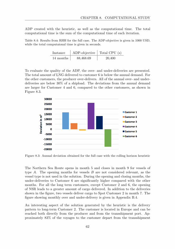
CHAPTER 8. COMPUTATIONAL STUDY
ADP created with the heuristic, as well as the computational time. The totalcomputational time is the sum of the computational time of each iteration.
Table 8.4: Results from RHH for the full case. The ADP-objective is given in 1000 USD,while the total computaional time is given in seconds.
Instance ADP-objective Total CPU (s)
14 months 88,468.69 20,400
To evaluate the quality of the ADP, the over- and under-deliveries are presented.The total amount of LNG delivered to customer 6 is below the annual demand. Forthe other customers, the producer over-delivers. All of the annual over- and under-deliveries are below 30% of a shipload. The deviations from the annual demandare larger for Customer 4 and 6, compared to the other customers, as shown inFigure 8.3.
Figure 8.3: Annual deviation obtained for the full case with the rolling horizon heuristic
The Northern Sea Route opens in month 5 and closes in month 9 for vessels oftype A. The opening months for vessels B are not considered relevant, as thevessel type is not used in the solution. During the opening and closing months, theunder-deliveries to Customer 6 are significantly higher compared with the othermonths. For all the long term customers, except Customer 2 and 6, the openingof NSR leads to a greater amount of cargo delivered. In addition to the deliveriesshown in the figure, two vessels deliver cargo to Spot Customer 2 in month 7. Thefigure showing monthly over and under-delivery is given in Appendix B.4.
An interesting aspect of the solution generated by the heuristic is the deliverypattern to long-term Customer 2. The customer is located in Europe and can bereached both directly from the producer and from the transshipment port. Ap-proximately 83% of the voyages to the customer depart from the transshipment
62

8.2. FULL CASE
port. The remaining voyages travel directly from the producer, and arrives in the2nd and 11th month. These months have a greater amount of over-deliveries to thecustomer.
Keep in mind that the rolling horizon heuristic constructs a solution by solving theproblem in sub-horizons. In order to evaluate the solution for the total planninghorizon, we should be aware of the behavior of the solutions found in the sub-problems. The computational time and gap found in each iteration, is summarizedbelow in Table 8.5. In iteration 2 and 3, the gap is less than 1%, and the compu-tational time is therefore below the maximum limit. Note that in iteration 4, thegap is significantly higher than the gap in the other iterations. In this iteration,the problem is solved for a time horizon from month 7 to month 11, where month7, month 8, and month 9 are within the central period. As seen from the figure inAppendix B.4, all of the customers are facing over-deliveries in month 7 and 8.
Table 8.5: Gap and time used in each iteration for the RHH
Instance Iteration Gap (%) Time in Iteration (s)
Full Case
1 4.50 3,600
2 0.55 < 100
3 1.00 2,300
4 77.32 3,600
5 7.95 3,600
6 5.85 3,600
7 10.62 3,600
Figure 8.4 displays the improving solutions found in each iteration. Despite thatfive of the iterations use the maximum time-limit, improving solutions after 500seconds was only found in iteration 5 and 6. In iteration 3, the best solution isfound after 230 seconds. During the next 2,000 seconds, the lower bound increasesand the iteration stops after approximately 2,300 seconds due to the value of thegap.
63

CHAPTER 8. COMPUTATIONAL STUDY
Figure 8.4: Solutions obtained in the iterations in RHH. The x-axis displays the compu-tation time for the solution, while the y-axis shows the objective-value for each solution.
The figure shows that for each iteration, the best solutions are remarkably differentin the objective value and in solution time. The objective value is a measure ofthe total costs for the time horizon within the iteration. The objective for an
64

8.3. AGGREGATED CASE
iteration also includes the cost of the total accumulated deviations in demands forthe frozen and central period. When the heuristic rolls over the sub-horizons fromone iteration to another, the frozen period increases. This implies that the totalaccumulated deviations in one iteration depends on accumulated deviations in theprevious iterations. However, in the last iteration, this cost is below 10% of theobjective for the best solution within the iteration.
As the sub-problems solve the problem for different months, seasonality is an im-portant aspect of the solutions. When the NSR is open, the travel times from theproducer to the customers are shorter, and in addition, it is possible to reach allcustomers within a month. With a lower travel time, more cargo is delivered toeach destination, and the sum of the daily costs decreases. When the cargo deliv-ered to each destination decreases, the total revenue per ship load delivered to thespot market also increases, due to the constant spot price.
Another important contribution to the objective value in the iterations is the in-going storage level. Recall from Section 6.1, that some information should betransferred from one iteration to another. The storage level at the producer andthe transshipment port are depended on the inventory level the previous day. Thestorage level the last day in the frozen period should therefore be known. Thisvalue is used to calculate the storage level the first day of the central period. If thein-going storage level is low, the amount of excess cargo available is small, and lesscargo can be delivered to the spot market during the central and forecast period.
Figure 8.4 can be used to evaluate the best solution found in iteration 4. As theNRS is open the first part of iteration, the best solution should be better than theone in iteration 5. In iteration 3 two spot sales occur in the central period andthe NSR is open during the whole sub-horizon. These two spot sales are the onlyspot sales included in the solution for the whole planning horizon. The solution initeration 4 should therefore be worse than best solution in iteration 3. Based onthe plots in Figure 8.4, we can conclude that the best objective in iteration 4 seemsreasonable if it is compared with the best solutions in the other iterations.The largegap in iteration 4 may be caused by the change of structure in the problem, whenthe NSR closes the first day of the forecast period.
8.3 Aggregated Case
In this section, we use the aggregation disaggregation heuristic (ADH) presented inChapter 6 to create an ADP. The ADH consists of two main components: solvingthe aggregated version of the full case and disaggregating the solution to producean ADP for the full case. As discussed in Chapter 6, several aggregation strategiesexist for this ADP planning problem. We test three different strategies for theinput in the ADH, and based on the results, we select the strategy that yields theADP with the lowest penalty costs.
65

CHAPTER 8. COMPUTATIONAL STUDY
8.3.1 Aggregation Strategies
Each aggregation strategy is solved by the exact method. The aggregation strate-gies are mainly based on geographic areas, but vary with respect to transshipmentfor customers located in Europe. As mentioned in Chapter 6, we choose two ge-ographic areas: Europe and Asia. Long-term customers located in Europe areclustered together, while long-term customers in Asia are clustered together. Theaggregated customers are denoted as LT-EU and LT-Asia respectively. Addition-ally, a spot customer is located in each geographic area. We test the followingstrategies:
• Strategy 1: 2 aggregated customers: LT-EU and LT-Asia. Only direct voy-ages to LT-EU are permitted.
• Strategy 2: 2 aggregated customers: LT-EU and LT-Asia. Transshipmentand direct voyages to LT-EU are permitted.
• Strategy 3: 1 aggregated customer: LT-Asia. The customers in Europe re-main individual customers, and voyages to Customer 1 can only be direct.
The strategies are visualized in Figure 8.5.
Figure 8.5: Aggregation Strategies
Table 8.6 shows the results from the aggregation strategies, where the computa-tional time (CPU) and optimality gap are from the exact method. The maximumtime limit is 36,000 seconds. The penalty costs are from the resulting ADP af-ter disaggregation. None of the strategies where solved to optimality within themaximum time limit. All of the strategies consider a 13-months planning horizon.
Table 8.6: Results from testing the aggregation strategies.
Aggregation strategy Penalty Costs CPU Exact (s) Optimality Gap Exact (%)
Strategy 1 21,754.56 36,000 9.15
Strategy 2 21,611.59 36,000 9.14
Strategy 3 13,071.06 36,000 16.7
66
8.3. AGGREGATED CASE
In order to evaluate and select the best strategy, we use the penalty costs anddeviations. After the disaggregation procedure, the operational costs are mostlikely to decrease as a result of the pessimistic travel times. However, the penaltycosts may increase due to changes in cargo delivered. We denote the resultingsolution after ADH as ADH-solution, while a solution from the aggregated case isdenoted as input solution.
Aggregation Strategy 1
The ADH with Strategy 1 produces an ADP with the highest penalty costs. Af-ter disaggregation, the penalty costs increase as a result of over-deliveries to thecustomers with travel times shorter than the aggregated travel times. Recall thatthe aggregated customers are assigned the most pessimistic travel times among thecustomers that constitute an aggregated customer. If the travel time of a reroutedvoyage is shorter than the pessimistic travel time, the amount of cargo delivered islarger due to decreased boil-off loss. This is problematic for the European customerwith the shorter travel times.
For the long-term customers in Asia, the differences in travel times are not as largeas for the case in Europe. In fact, the difference between the one-way pessimistictravel time and the shortest travel time among the Asian customers is 2 days.Among the European customers on the other hand, the difference is 4 days.
In Chapter 6, we discuss the possibility of premature arrival dates after disaggrega-tion, as a result of the conservative travel times in the aggregated case. One of thererouted voyages in the ADH solution is affected by the large spread in travel timesamong the customers in Europe. Here, the original voyage to LT-EU has an arrivaltime during month m. When the voyage is rerouted to Customer 1, the new arrivaltime ends up in month m-1, because of the large difference in travel times. Cus-tomer 1 has already been assigned a delivery from a voyage with arrival in monthm-1, so the heuristic reroutes the voyage to Spot Customer 1 instead, resulting inunder-delivery for Customer 1 in month m. We carry out a post-processing stepto rectify this. We postpone the departure day of the voyage with at least thedifference between the pessimistic travel time and the travel time to Customer 1,TLTEU – TCustomer1 days, as long as the postponed voyage is inventory, routingand berth feasible.
67

CHAPTER 8. COMPUTATIONAL STUDY
Figure 8.6: Annual deviation after ADH, given aggregation with Strategy 1
In Figure 8.6, the annual deviations after disaggregation are presented. The sub-stantial amount of over-delivery to Customer 2 is a result of the occurrences ofover-deliveries every month. Since Customer 2 and LT-EU have the same traveltimes, one would therefore assume that the change in deviation between the ag-gregated case and Customer 2 would be smaller. However, the monthly demandof Customer 2 is smaller than the cargo delivered in a given month, leading toover-deliveries. Customer 1, on the other hand, has a larger monthly demand andshorter travel time. The amount of cargo delivered each month is not far from thedemand, which leads to small over-deliveries.
Customer 4 experiences quite a big amount of under-deliveries in months 6, 7 and10 due to the vessel choice in the input solution (see Appendix B.2). Vessels oftype B, which have lower tank capacities, are used in month 6 and 7, and arererouted to Customer 4. In the input solution, the voyages carried out with vesselsof type B have the departure day in the previous month and arrival day in thenext. The departure day determines the travel time and consequently the amountof cargo delivered. Since the travel time in the departure month is longer than inthe arrival month, the amount of cargo delivered is smaller. The cargo deliveredfrom this voyage in combination with the other deliveries that are made with vesselsof type A in the arrival month, is close to the aggregated demand. But when thevoyages are disaggregated, the deliveries made by vessels of type B deviate fromthe demand of the individual customers in Asia. As a result of this, Customer 4experiences large under-deliveries in months 6 and 7.
In month 10, a conventional vessel with the smallest capacity in the fleet is sentto LT-Asia. The conventional vessels with both larger capacity and best cost-to-capacity ratio are at this time occupied, so the smallest conventional, which hasthe second best in cost-to-capacity ratio, is therefore sent instead. Here, a similarproblem, where differences between the cargo delivered and individual demandafter disaggregation as a result of vessel choice, occurs. The small conventionalvessel is rerouted to Customer 4, which explains the substantial under-delivery inmonth 10.
68

8.3. AGGREGATED CASE
The monthly demand of Customer 6 is the largest among the customers in Asia.After the disaggregation, Customer 6 experiences large monthly under-deliveriesmore frequently due to difference in cargo delivered and vessel capacity. If wecompare the deviation with the full case 13-months instance solved by exact method(see Figure 8.2) and by the RHH (see Figure 8.3), Customer 6 faces a large annualunder-delivery in these solutions as well. This shows that it is challenging tosatisfy the monthly demand of Customer 6 due to differences in demand and vesselcapacity.
Besides the large spread in travel times for the European customers, another short-coming with this strategy is that transshipment to customers in Europe is not per-mitted. The purpose of using transshipment as a way of transferring cargo ontoconventional vessels is ignored. For this reason, we do not proceed further withStrategy 1.
Aggregation Strategy 2
In this aggregation strategy, transshipment is added as a possibility for the ag-gregated customer in Europe. There are some similarities in the ADH-solutionproduced with Strategy 2 as in the ADH-solution produced from Strategy 1.
The direct voyages to LT-EU remains the dominating routing choice from theaggregated solution, where 87.5% of the voyages to LT-EU are direct. The reasonbehind is the aggregated demand. Here, the sum of the direct deliveries in a givenmonth to LT-EU is closer to the monthly aggregated demand than the deliveries viatransshipment. Recall that the conventional vessels have smaller capacities thanthe ice-going vessels and deliver less in every voyage. So, when a direct voyage isrerouted to Customer 2, the delivery volume is larger than the monthly demand,which in turn leads to over-deliveries. The few transshipment voyages to the LT-EUoccurring in the solution are rerouted to Customer 2, since voyages to Customer 1can only be direct.
Unlike the ADH-solution from the aggregated case with Strategy 1, all of the indi-vidual customers in Asia receive under-deliveries on an annual basis. In this case,the main reason behind is the input solution, where Customer LT-Asia experienceunder-deliveries more frequently compared to the input solution from Strategy 1.This leads to increased under-deliveries to Customer 3, 5 and 6. Customer 4 doesnot suffer from the choice of vessels as much as in the previous input solution withStrategy 1, and hence the amount of under-deliveries has decreased substantially.If we compare the vessel choice for the month where one of the deliveries to LT-Asiaare made with a vessel of type B in Strategy 1, we see that only vessels of type Aare used, and departure and arrival times are in the same month. Therefore, thevessel choice is better in the input solution of Strategy 2.
69

CHAPTER 8. COMPUTATIONAL STUDY
Figure 8.7: Annual deviation after ADH, given aggregation with Strategy 2
A drawback with this strategy is when voyages to LT-EU only use transshipment ina given month. These voyages cannot be rerouted to Customer 1 without modifyingthe other decision variables. A potential rerouting to Customer 1 implies that thecargo picked up and cargo delivered values need to be changed to prevent inventoryinfeasibility at the production and transshipment storage tanks. The disaggregationprocedure would therefore reroute voyages to a spot customer instead Customer 1,which leads to an under-delivery.
Aggregation Strategy 3
We see that the aggregation of the two long-term customers in Europe in accor-dance with strategies 1 and 2 lead to substantial over-deliveries for the individ-ual customers after disaggregation. The ADH-solutions of both strategies containconsiderable over-deliveries for the individual customers in Europe. Additionally,Strategy 1 overlooks the transshipment aspect of the planning problem for the Eu-ropean customers. As a consequence of these factors, Strategy 3 only aggregatesthe long-term customers in Asia.
As Table 8.6 shows, the total penalty costs are much lower with Strategy 3, sincethe travel times and demands of the individual customers in Europe are now takeninto account when solving the aggregated case by exact method. Around 83% ofthe voyages go to Customer 2 go via the Transshipment port, where the cargois transferred onto a conventional vessel with smaller capacity than the ice-goingvessel. The cargo delivered by the conventional vessel is closer to the monthlydemand of Customer 2, compared to the direct voyages from previous strategies.As shown in Figure 8.8, the monthly deviations for the customers in Europe aremuch smaller compared to the results from the aggregated cases with Strategy 1and 2.
70

8.3. AGGREGATED CASE
Figure 8.8: Annual deviation after ADH, given aggregation with Strategy 3
The annual deviations for customers 1, 2 and 3 are reduced when Strategy 3 isused, compared to Strategy 1 and 2. Because of frequent over-deliveries to LT-Asia in the input solution, Customer 4 and 5 receive frequent over-deliveries aswell, leading to an over-delivery on an annual basis. On the other hand, Customer6, who has the largest demand among the customers in Asia, experiences frequentunder-deliveries in all of the strategies.
Note that the gap from solving the aggregated case with Strategy 3 is slightly worsecompared to the gaps of the other aggregation strategies. Since the customers inEurope are not aggregated, the complexity increases due to the increased numberof nodes in the problem, thus increasing the computational effort. However, thepenalty costs are lower than the penalty costs from the other strategies, whichmakes the solution a good input for the disaggregation procedure.
Since Strategy 3 discerns between the European long-term customers by takingtransshipment explicitly into account and has lower penalty costs, we choose toproceed with this aggregation strategy.
8.3.2 ADH
So far, the aggregated case has been solved by exact method. The result is usedas input to the disaggregation procedure to create a solution for the full case. Thecomputational time of the disaggregation procedure is minimal, which implies thatthe solution method used to solve the aggregated case is the sole contributor to thecomputational time of the ADH. Based on the results in Table 8.6, we see that theexact method is time consuming. Considering that the RHH is able to solve theADP planning problem quicker than the exact method, we use the RHH to solvethe aggregated case before disaggregation.
The combination of RHH and ADH is denoted as RHH-ADH, while the combina-
71

CHAPTER 8. COMPUTATIONAL STUDY
tion of exact method and ADH is denoted as E-ADH. In order to compare thesetwo solution method combinations, the E-ADH is solved for a 14-month planninghorizon like the RHH-ADH. Since we are only interested in a 12-month ADP, weremove the start-up month and the last month from the results to get an ADP-objective. The results from both solution method combinations are presented belowin Table 8.7.
Table 8.7: Solutions from the ADH without post-processing. The ADP-objective is givenin 1000 USD and the CPU in seconds.
Solution Method ADP-objective CPU (s)
E-ADH 91,724.041 36,000
RHH-ADH 102,047.131 18,150
The objective value of RHH-ADH is worse compared to the objective value ofE-ADH. The input solution from the RHH has more frequent under-deliveries toLT-Asia than the input solution from the exact method. Monthly over- and under-deliveres are displayed in Figure 8.10. In the RHH-ADH solution, the difficultiesarise in months 6, 7 and 12. In month 7, Customer 3 and 6 suffer from substantialunder-deliveries, while Customer 5 experiences quite a big under-delivery in month12. The big under-delivery in month 12 is a result of the input solution, where themonthly deviation to LT-Asia is about 18,000m3 in under-delivery. Customer 4, onthe other hand, receives almost twice the amount of over-delivery in the RHH-ADHsolution as in the E-ADH solution, which is illustrated in Figure 8.9.
Figure 8.9: Annual deviation from E-ADH and RHH-ADH
Destination Swap
To reduce the over- and under-deliveries, we consider the possibilities for modifyingthe destinations of some of the voyages in the ADH-solution. The fleet of vessels isheterogeneous and by swapping the rerouted destination for vessels heading to the
72

8.3. AGGREGATED CASE
same geographic area, we may reduce some of the over- or under-deliveries. A swapimplies a switch of the destination between two voyages. When two destinationsare swapped, we must ensure that the new arrival days are in the same month asin the ADH-solution before the swap.
In the solution obtained from E-ADH, we see that Customer 4 receives substantialover-deliveries, while Customer 6 faces substantial under-deliveries. Therefore, weswap some of the voyages between Customer 4 and 6, in an attempt to improve thesolution. Figure 8.10 depicts the monthly over- and under-deliveries. We see thatit is beneficial to swap the voyages with arrival days in month 9, 10 and 12 for thesecustomers due to the difference in the vessels’ capacities. These rearrangements ofthe departures decreases the costs of under- and over-delivery with 14.0%.
Figure 8.10: Monthly deviations from E-ADH and RHH-ADH before destination swap
73

CHAPTER 8. COMPUTATIONAL STUDY
In the solution given by RHH-ADH, we evaluate the departures to Customer 3,4 and 6, as these customers are suffering from the highest deviations. Three ofthe departures to Customer 4 can be switched with two departures to Customer6, and one to Customer 3. This post-processing step decreases the cost of under-and over-delivery by 11.8%.
Table 8.8 below shows how the post-processing of the solutions decreases the ADP-objective. The new annual deviations are illustrated in Figure 8.11. Note that thepost-processing of the solutions has decreased the over-delivery to Customer 4 andthe under-delivery to Customer 6 significantly for both the E-ADH and RHH-ADH.
Table 8.8: Solutions from the ADH before and after destination swaps
Solution Method ADP-objective before swaps ADP-objective after swaps
E-ADH 91,724.041 89,475.70
RHH-ADH 102,047.131 99,014.31
Figure 8.11: Annual deviations after post-processing the ADH solutions
The resulting ADP from RHH-ADH is not as cost-efficient as the ADP createdwith E-ADH. However, as Table 8.7 and 8.8 depict, RHH-ADH only uses half ofthe computational time of E-ADH to produce a solution, whereas E-ADH stopswhen the maximum time limit is reached.
The RHH has a maximum time limit for each iteration and produces an ADP in ashorter amount of time compared to exact method. An advantage with the RHH isthat we can adjust the time limit on the iterations, which makes it flexible to use.A longer iteration time length may lead to an ADP of higher quality, while shortiteration time lengths may reduce the quality. The RHH is also more predictablethan the exact method, in the sense that we have an upper bound on how long ittakes to create an ADP since we operate with a time limit for each iteration.
74
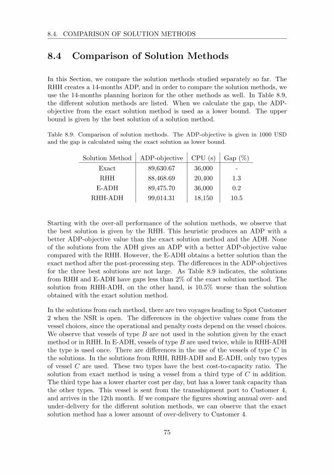
8.4. COMPARISON OF SOLUTION METHODS
8.4 Comparison of Solution Methods
In this Section, we compare the solution methods studied separately so far. TheRHH creates a 14-months ADP, and in order to compare the solution methods, weuse the 14-months planning horizon for the other methods as well. In Table 8.9,the different solution methods are listed. When we calculate the gap, the ADP-objective from the exact solution method is used as a lower bound. The upperbound is given by the best solution of a solution method.
Table 8.9: Comparison of solution methods. The ADP-objective is given in 1000 USDand the gap is calculated using the exact solution as lower bound.
Solution Method ADP-objective CPU (s) Gap (%)
Exact 89,630.67 36,000 -
RHH 88,468.69 20,400 1.3
E-ADH 89,475.70 36,000 0.2
RHH-ADH 99,014.31 18,150 10.5
Starting with the over-all performance of the solution methods, we observe thatthe best solution is given by the RHH. This heuristic produces an ADP with abetter ADP-objective value than the exact solution method and the ADH. Noneof the solutions from the ADH gives an ADP with a better ADP-objective valuecompared with the RHH. However, the E-ADH obtains a better solution than theexact method after the post-processing step. The differences in the ADP-objectivesfor the three best solutions are not large. As Table 8.9 indicates, the solutionsfrom RHH and E-ADH have gaps less than 2% of the exact solution method. Thesolution from RHH-ADH, on the other hand, is 10.5% worse than the solutionobtained with the exact solution method.
In the solutions from each method, there are two voyages heading to Spot Customer2 when the NSR is open. The differences in the objective values come from thevessel choices, since the operational and penalty costs depend on the vessel choices.We observe that vessels of type B are not used in the solution given by the exactmethod or in RHH. In E-ADH, vessels of type B are used twice, while in RHH-ADHthe type is used once. There are differences in the use of the vessels of type C inthe solutions. In the solutions from RHH, RHH-ADH and E-ADH, only two typesof vessel C are used. These two types have the best cost-to-capacity ratio. Thesolution from exact method is using a vessel from a third type of C in addition.The third type has a lower charter cost per day, but has a lower tank capacity thanthe other types. This vessel is sent from the transshipment port to Customer 4,and arrives in the 12th month. If we compare the figures showing annual over- andunder-delivery for the different solution methods, we can observe that the exactsolution method has a lower amount of over-delivery to Customer 4.
75

CHAPTER 8. COMPUTATIONAL STUDY
In general, the solutions obtained with the RHH have a higher amount of over-and under-deliveries compared to the solutions obtained with the exact solutionmethod. For the RHH and the exact solution method there are small differencesin total under-deliveries, but the RHH solution delivers approximately 15,000m3
more to the customers than the solution of the exact method. Recall from Section8.3.2 that this is also the case for the ADH. After the disaggregation procedure,the over- and under-deliveries increase. Despite the increase in deviations, it isworth mentioning that none of the customers in all of the solutions suffer from adeviation of more than half a ship load.
The delivery pattern to long-term Customer 2 differs in each solution. Customer 2can be reached directly from the producer and from the transshipment port. In thesolutions from the exact method, RHH, and E-ADH, the same delivery pattern tothe customer is created, where 83.5% of the arrivals departs from the transshipmentport. These voyages use the same type of vessel C. In the RHH-ADH solution,the number of voyages departing from the transshipment port to the customer is75%. Figure 8.9 and 8.11 show that a reduction in voyages departing from thetransshipment port leads to increased over-deliveries to the customer. This is dueto the transfer of cargo onto a smaller conventional vessel with a capacity closer tothe monthly demand of the customer.
Table 8.9 also shows the computational time for the solutions. The RHH-ADH usethe shortest computational time to create an ADP. Recall that the computationaltime for the disaggregation procedure is reckoned to be minimal, so the compu-tational time of solving for the aggregated case is the main contributor. Becausethe number of nodes are reduced in the aggregated case, the computational timeof solving the aggregated case with RHH is shorter than solving the full case withRHH. In both cases, two of the iterations reached the optimality gap limit, butfor the aggregated case this occurs faster than for the full case. Both the exactsolution method and E-ADH have a computational time of 36,000 seconds.
The RHH provides a better solution within a shorter amount of time, than theexact method. A drawback with the heuristic is that in each iteration, only a partof the total planning horizon is evaluated. Deliveries to the customers are adjustedfor over and under-deliveries in earlier iterations, but deliveries in the consecutiveiterations are not considered. As we can see from Figure 8.4, the quality of thesolutions found in each iteration depend on seasonality. Recall from Section 8.2.2,that when the NSR closed between the central and the forecast period, the gapwas significant higher compared to the other iterations. The somewhat myopicexploration of the planning horizon in combination with seasonal effects in routingchoice, may be the reason behind the higher amount of over and under-deliveries.In spite of the RHH creating what we consider good solutions for the ADP-problem,these solutions may not be suitable as input in the ADH due to the higher amountof over and under-deliveries.
The ADH improves the operational costs from the input solution due to the pes-
76
8.4. COMPARISON OF SOLUTION METHODS
simistic travel times, but the deviations from annual demand are not improved.When the RHH-ADH reroutes the vessels, the deviations increase compared tothe aggregated input solution. For E-ADH, the total difference in over and- under-deliveries are small compared with the exact method. The amount of over-deliveriesare 8000m3 less than the exact method, while the under-deliveries are 2000m3 more.Despite the deviations, the E-ADH provides a better objective than the exact so-lution within the same computational time.
The biggest advantage with the ADH, is that the computational time dependsonly on the computational time of the aggregated solution. The aggregated case issmaller and hence the complexity is significantly lower compared to the full case.As the RHH obtains a solution faster for the aggregated case than for the fullcase, this improves the solution time for the RHH-ADH. However, the reduction ofcomputation time comes at the expense of the solution quality. The ADH providesbetter results after the post-processing of the departures, but the solution is worsecompared to the solutions from other methods.
In order to evaluate the total performance of the solution methods, the intended useof the ADP can be considered. The ADP can either be a draft used for negotiationswith the customers, or a suggested plan made after the negotiations. If the ADP isused as a draft, the ADH can be useful due to the computational time. RHH-ADHhave the shortest computational time and can produce an ADP faster than theother solution methods. RHH is the best option if the ADP is should be optimizedafter the negotiations. Even though the RHH does not solve the ADP planningproblem with the shortest computational time, it produces the most cost-efficientADP.
77

CHAPTER 8. COMPUTATIONAL STUDY
78
Chapter 9
Concluding Remarks
The problem in this thesis is to solve an annual delivery program (ADP) planningproblem for an LNG producer with a heterogeneous fleet of vessels. The goal is tocreate an ADP that fulfills the contractual demands at a minimum cost. Operativecosts for the vessels and penalty costs related to over- and under-deliveries areincluded in the objective. Revenue from selling excess LNG in the spot markets isconsidered as a negative cost.
The producer is located north of the Arctic Circle, while the customers can befound in different areas of the world. Specialized ice-going vessels travel fromthe producer either directly to the customers or to a transshipment port. TheNorthern Sea Route is used to reach customers located in Asia directly. When theroute is closed, the ice-going vessels must travel to Europe and unload the cargoat the transshipment port. From this port, conventional LNG-vessels are usedfor delivery to the customers in Asia. The problem is formulated as a mixedinteger programming (MIP) model that allow partial loading when the vesselsare traveling from the producer to the transshipment port. The purpose of thisthesis is to use heuristic approaches to minimize the costs of the ADP. Solutiontime is also an important consideration for the producer, and should be evaluatedalong with the objective value. Three different solution methods are tested andcompared to find the best solution for the problem. The exact solution methodusing branch-and-bound did not obtain a gap below 10% within a computationaltime of 36,000 seconds. Two heuristics are used to create better solutions andreduce the computational time. The first one tested, is a rolling horizon heuristic(RHH), similar to the one presented in Rakke et al. (2011). The RHH reduces boththe computational time and the objective value compared to the exact solutionmethod.
An aggregation disaggregation heuristic (ADH) is developed to reduce the compu-tational time even further. In the ADH, the customers are aggregated accordingto an aggregation strategy. The aggregated case is then solved with the exactsolution method (E-ADH) and RHH (RHH-ADH). Afterwards, the solutions are
79
CHAPTER 9. CONCLUDING REMARKS
disaggregated.
The performance of the ADH depends on several factors:
• Aggregation strategy: after testing different aggregation strategies, the strat-egy leading to best results includes an aggregation of customers based ongeography and routing choice.
• Solution method used for the aggregated case: as the computational timein the disaggregation procedure is minimal, the total computational time forthe heuristic depends on the time used to solve the aggregated case.
• Over- and under-deliveries in the solution for the aggregated case: the com-putational study in Chapter 8 shows that the amount of over- and under-deliveries increases after the disaggreation procedure. For the ADH to be ableto produce high quality solutions, the amount of over- and under-deliveriesin the input solution from the aggregated case should be limited.
The results obtained from the ADH differ. The E-ADH obtained better solutionswithin the same computational time as the exact method. For RHH-ADH thecomputational time is further decreased, but the objective value is worse. NeitherE-ADH or RHH-ADH yields a better objective value than RHH. RHH-ADH, onthe other hand, solves the problem with shorter computational time than RHH dueto the aggregation.
The aggregated case has a reduced complexity compared to the full case, and asdescribed in Chapter 8, the RHH produces a solution faster for the aggregatedcase. The RHH-ADH can thus be a suitable decision tool when quick feedbackis important. In addition, if the decision maker is familiar with an estimateddistribution of the demand, and want to obtain solutions for alternative demandscenarios, the ADH is well suited. Once a solution for the aggregated case is found,solutions for different distributions of the demand within the aggregated customersare quickly obtained.
80
Chapter 10
Future Research
There are several areas of improvement when it comes to solving the ADP planningproblem.
Two heuristic solutions methods have been developed to create an Annual DeliveryProgram effectively. The quality of the solution from the Aggregation Disaggrega-tion Heuristic (ADH) highly depends the input solution from the aggregated case.The penalty costs increase after disaggregation, so if the input solution has largedeviations, the solution after disaggregation becomes worse. The vessel choice inthe input solution is not optimal for the disaggregated solution due to different in-dividual customer demands. A vessel combination may be close to the demand ofan aggregated customer, but during disaggregation, the vessels are assigned to cus-tomers to avoid premature deliveries. A vessel with smaller capacity that is oftenrerouted to a customer with higher demand leads to substantial under-deliveriesannually. Therefore, departure times should be modified to avoid considerablepenalty costs. Therefore, the ADH can be improved with a re-optimization proce-dure after disaggregation, such as a neighborhood search heuristic or a MIP-basedimprovement heuristic, to modify vessel choice and departure times.
Matheuristics is a more recent solution methodology within the field of heuristic so-lution approaches. Here, mathematical programming concepts are combined withheuristics used to create or improve solutions. A neighborhood search in combi-nation with a matheuristic could have been added on top the ADH and RHH toimprove the solutions.
An interesting extension to the ADP planning problem is disrupting management.The Northern Sea Route is characterized by varying sea ice levels and uncertaintyin weather conditions, which introduces the potential for creating robust ADPs. Byincluding uncertainty in travel times, the producer needs to re-schedule an ADP tominimize the costs of disruption. The ADP planning problem can be reformulatedas a two-stage stochastic model, where the first stage generates an initial ADP,while the second stage is a recourse problem that re-optimizes the ADP based on
81
CHAPTER 10. FUTURE RESEARCH
the realization of stochastic parameters.
The rolling horizon heuristic (RHH) can be adapted to a scenario based approachthat solves a two-stage stochastic ADP planning problem. As the heuristic rollsover, a scenario is realized with a probability distribution. Based on new infor-mation that arrives in every central period, the recourse problem is solved, andpredictions are made for the rest of the horizon. Considering the length of theplanning horizon, a RHH approach for a two-stage stochastic ADP planning prob-lem sems ideal.
Another solution method to a two-stage stochastic ADP planning problem is tocombine optimization with simulation. In this case, the simulation procedure isused to evaluate the solution from the optimization procedure. The simulationprocedure should then re-optimize the proposed schedule as a consequence of sce-nario realizations.
82

Bibliography
H. Andersson, M. Christiansen, G. Desaulniers, and J. G. Rakke. Creating annualdelivery programs of liquefied natural gas. Optimization and Engineering, 18(1):299–316, Mar 2015. ISSN 1573-2924. doi: 10.1007/s11081-015-9305-y.
I. H. Bugge and M. Thavarajan. Creating an Annual Delivery Program For anLNG Producer with Transshipment. Project Report, Dec 2017.
CHNL. Icebreakers Assistance, 2018a. URL http://www.arctic-lio.com/nsr icebreakersassistance. (Accessed: June 7th, 2018).
CHNL. Admittance criteria and Icebreaker Tariffs, 2018b. URL http://
www.arctic-lio.com/nsr tariffsystem. (Accessed: Dec 3th, 2017).
CHNL. Ice Class Criteria, 2018c. URL http://www.arctic-lio.com/nsr iceclasscriteria. (Accessed: June 7th, 2018).
CHNL. NSR - General Area Description, 2018d. URL http://www.arctic-lio.com/nsr generalareadescription. (Accessed: June 7th, 2018).
M. Christiansen. Decomposition of a combined inventory and time constrainedship routing problem. Transportation Science, 33(1):3–16, 1999. ISSN 00411655,15265447. URL http://www.jstor.org/stable/25768842.
M. Christiansen, K. Fagerholt, B. Nygreen, and D. Ronen. Chapter 4 Mar-itime Transportation. In Transportation, volume 14 of Handbooks in Opera-tions Research and Management Science, pages 189 – 284. Elsevier, 2007. doi:https://doi.org/10.1016/S0927-0507(06)14004-9.
M. Christiansen, K. Fagerholt, B. Nygreen, and D. Ronen. Ship routing andscheduling in the new millennium. European Journal of Operational Re-search, 228(3):467 – 483, 2013. ISSN 0377-2217. doi: https://doi.org/10.1016/j.ejor.2012.12.002.
B. Dinsmore. A Guide to Understanding Ship Weight and Tonnage Measurements,2011. URL http://www.themaritimesite.com/a-guide-to-understanding-ship-weight-and-tonnage-measurements/. (Accessed: June 7th, 2018).
DNV GL AS. Sloshing analysis of LNG membrane tanks, february edition, Feb2016. URL https://rules.dnvgl.com/docs/pdf/DNVGL/CG/2016-02/DNVGL-CG-0158.pdf. (Accessed: May 3rd 2018).
83

BIBLIOGRAPHY
M. P. Dodds. The difference with LNG? It’s about boil-off isn’t it? Technical re-port, Reed Smith, 2014. URL https://www.reedsmith.com/en/perspectives/2014/06/the-difference-with-lng--its-just-about-boiloff-is. (Ac-cessed: June 7th, 2017).
EIA. Arctic Oil and Natural Gas Resources, January 2012. URL https://
www.eia.gov/todayinenergy/detail.php?id=4650. (Accessed: Dec 19th 2017).
EIA. International Energy Outlook 2017, sep 2017a. URL https://www.eia.gov/outlooks/ieo/. (Accessed: June 7th, 2017). Report Number: DOE/EIA-0484(2017).
EIA. How much carbon dioxide is produced when different fuels are burned?,Jun 2017b. URL https://www.eia.gov/tools/faqs/faq.php?id=73&t=11. (Ac-cessed: June 8th 2018).
A. Fredheim and E. Solbraa. Gas Processing Part 1, Offshore gas processing forrich gas transport. In TEP4185-Natural Gas Technology. NTNU Department ofEnergy and Process Engineering, 2016.
GIIGNL. LNG Information Paper No. 3 LNG Ships. Technical report, The In-ternational Group of Liquefied Natural Gas Importers, 92200 Neuilly-sur-Seine,France, 2009.
GIIGNL. The LNG industry GIIGNL ANNUAL REPORT 2017. Technical report,The International Group of Liquefied Natural Gas Importers, 92200 Neuilly-sur-Seine, France, 2017.
GIIGNL. The LNG industry GIIGNL ANNUAL REPORT 2018. Technical report,The International Group of Liquefied Natural Gas Importers, 92200 Neuilly-sur-Seine, France, 2018.
H. Gloystein. Factbox: The three sticking points of long-term LNG contracts,February 2018. URL https://www.reuters.com/article/us-asia-lng-arbitration-factbox/factbox-the-three-sticking-points-of-long-
term-lng-contracts-idUSKBN1FX0MM. (Accessed: May 5th, 2018).
V. Goel, K. C. Furman, J.-H. Song, and A. S. El-Bakry. Large neighborhood searchfor lng inventory routing. Journal of Heuristics, 18(6):821–848, Dec 2012. ISSN1572-9397. doi: 10.1007/s10732-012-9206-6. URL https://doi.org/10.1007/s10732-012-9206-6.
R. Grønhaug and M. Christiansen. Supply Chain Optimization for the LiquefiedNatural Gas Business. In J. A. Nunen, M. G. Speranza, and L. Bertazzi, editors,Innovations in Distribution Logistics, pages 195–218, Berlin, Heidelberg, 2009.Springer Berlin Heidelberg. ISBN 978-3-540-92944-4.
R. Grønhaug, M. Christiansen, G. Desaulniers, and J. Desrosiers. A Branch-and-Price Method for a Liquefied Natural Gas Inventory Routing Problem. Trans-portation Science, 44(3):400–415, 2010. ISSN 00411655, 15265447.
84

BIBLIOGRAPHY
E. E. Halvorsen-Weare and K. Fagerholt. Routing and scheduling in a liquefiednatural gas shipping problem with inventory and berth constraints. Annals ofOperations Research, 203(1):167–186, Mar 2013. ISSN 1572-9338. doi: 10.1007/s10479-010-0794-y.
E. E. Halvorsen-Weare, K. Fagerholt, and M. Ronnqvist. Vessel routing andscheduling under uncertainty in the liquefied natural gas business. Comput-ers & Industrial Engineering, 64(1):290 – 301, 2013. ISSN 0360-8352. doi:https://doi.org/10.1016/j.cie.2012.10.011.
International Gas Union. 2017 World LNG Report, 2017. URLhttps://www.igu.org/sites/default/files/103419-World IGU Report no%
20crops.pdf. (Accessed: Sep 29th, 2017).
R. Kantharia. How Does LNG Terminal Works?, 2016. URL http://
www.marineinsight.com/ports/how-does-lng-terminal-works/. (Accessed:Sep 27th, 2017).
J. F. Kuo, R. B. Campbell, Z. Ding, S. M. Hoie, A. J. Rinehart, R. E. Sandstrom,T. W. Yung, M. N. Greer, and M. A. Danaczko. LNG Tank Sloshing AssessmentMethodology – The New Generation. In Proceedings of the Nineteenth (2009)International Offshore and Polar Engineering Conference. International Societyof Offshore and Polar Engineers, June 2009. ISSN 1098-618.
S. A. Lawrence. International Sea Transport: The Years Ahead. 1972. ISBN0669843199.
J. Lee and B.-I. Kim. Industrial ship routing problem with split delivery and twotypes of vessels. Expert Systems with Applications, 42(22):9012 – 9023, 2015.ISSN 0957-4174. doi: https://doi.org/10.1016/j.eswa.2015.07.059.
A. A. Lopac. Recent trends in transporting of LNG, liquefied natural gas. InICTS2008-Transport Policy, 2008.
Marine Traffic. Voyage Planner, 2018. URL https://www.marinetraffic.com/no/voyage-planner. (Accessed: June 7th, 2018).
C. Merce and G. Fontan. MIP-based heuristics for capacitated lotsizing problems.International Journal of Production Economics, 85(1):97 – 111, 2003. ISSN0925-5273. doi: https://doi.org/10.1016/S0925-5273(03)00090-2. Planning andControl of Productive Systems.
S. Mokhatab, J. Y. Mak, J. V. Valappil, and D. A. Wood. Handbook of LiquefiedNatural Gas. Gulf Professional Publishing, 2014. ISBN 9780124045859. doi:https://doi.org/10.1016/C2011-0-07476-8.
F. Mutlu, M. K. Msakni, H. Yildiz, E. Sonmez, and S. Pokharel. A comprehensiveannual delivery program for upstream liquefied natural gas supply chain. Euro-pean Journal of Operational Research, 250(1):120 – 130, 2016. ISSN 0377-2217.doi: https://doi.org/10.1016/j.ejor.2015.10.031.
85

BIBLIOGRAPHY
National Snow & Ice Data Center. Sea Ice Index Animation Tool, 2018. URLhttp://nsidc.org/data/seaice index/archives/image select. (Accessed:June 7th, 2018).
J. Pettersen. Compendium LNG Technology 3rd edition. In TEP4185-Natural GasTechnology. NTNU Department of Energy and Process Engineering, 2016.
J. G. Rakke, M. Stalhane, C. R. Moe, M. Christiansen, H. Andersson, K. Fager-holt, and I. Norstad. A rolling horizon heuristic for creating a liquefied naturalgas annual delivery program. Transportation Research Part C: Emerging Tech-nologies, 19(5):896 – 911, 2011. ISSN 0968-090X. doi: https://doi.org/10.1016/j.trc.2010.09.006. Freight Transportation and Logistics (selected papers fromODYSSEUS 2009 - the 4th International Workshop on Freight Transportationand Logistics).
J. G. Rakke, H. Andersson, M. Christiansen, and G. Desaulniers. Branch-price-and-cut for creating an annual delivery program of multi-product liquefied naturalgas. Les Cahiers du GERAD, Apr 2012. ISSN 0711–2440.
D. F. Rogers, R. D. Plante, R. T. Wong, and J. R. Evans. Aggregation and Disag-gregation Techniques and Methodology in Optimization. Operations Research,39(4):553–582, 1991. ISSN 0030364X, 15265463. URL http://www.jstor.org/stable/171164.
H. Schøyen and S. Brathen. The northern sea route versus the suez canal: casesfrom bulk shipping. Journal of Transport Geography, 19(4):977 – 983, 2011. ISSN0966-6923. doi: https://doi.org/10.1016/j.jtrangeo.2011.03.003.
Y. Shao, K. C. Furman, V. Goel, and S. Hoda. A hybrid heuristic strategyfor liquefied natural gas inventory routing. Transportation Research Part C:Emerging Technologies, 53:151 – 171, 2015. ISSN 0968-090X. doi: https://doi.org/10.1016/j.trc.2015.02.001.
Q. Shen, F. Chu, and H. Chen. A lagrangian relaxation approach for a multi-mode inventory routing problem with transshipment in crude oil transportation.Computers & Chemical Engineering, 35(10):2113 – 2123, 2011. ISSN 0098-1354.doi: https://doi.org/10.1016/j.compchemeng.2011.01.005.
M. Stalhane, J. G. Rakke, C. R. Moe, H. Andersson, M. Christiansen, and K. Fager-holt. A construction and improvement heuristic for a liquefied natural gas in-ventory routing problem. Computers & Industrial Engineering, 62(1):245 – 255,2012. ISSN 0360-8352. doi: https://doi.org/10.1016/j.cie.2011.09.011.
Suez Canal Authority. Marketing Policies, 2017a. URLhttps://www.suezcanal.gov.eg/English/Tolls/Pages/MarketingPoliciesAndTollRebates.aspx. (Accessed: June 7th, 2018).
Suez Canal Authority. Tolls Calculator, 2017b. URL https:
//www.suezcanal.gov.eg/English/Tolls/Pages/TollsCalculator.aspx.(Accessed: Dec 3th, 2017).
86

BIBLIOGRAPHY
J.-F. Tremblay. China looks to restore the blue skies. Chemical & EngineeringNews, 95(26):30–34, June 2017. URL https://cen.acs.org/articles/95/i26/China-looks-restore-blue-skies.html. (Accessed: June 7th, 2017).
M. D. Tusiani and G. Shearer. LNG: A Nontechnical Guide. Penwell Corporation,Tulsa, Oklahoma, USA, 2007. ISBN 978-0-87814-885-1.
M. S. Zakaria, K. Osman, and M. N. Musa. Boil-Off Gas Formation inside LargeScale Liquefied Natural Gas (LNG) Tank Based on Specific Parameters. AppliedMechanics and Materials, 229-231:690–694, 2012.
87

BIBLIOGRAPHY
88

Appendices
89


Appendix A
Derivation of Boil-OffConstraints
In this appendix αijvt and βijvt in constraints (5.14) are derived. In order to derivethe expressions, some new notation are introduced. In addition, some of the indicesare reduced in order to simplify the notation during the derivation.
Let lt describe the inventory level at a vessel when traveling between the producerand the transshipment port. Note that the definition of lt differs from the definitionof lijvt used in Section 5.4. lijvt is the cargo loaded onto the vessel, while lt is the
cargo on board the vessel when traveling. In this section, we let l0 be the amountof cargo loaded onto the vessel. The inventory level in a vessel when travelingbetween two ports is given by:
lt+1 = (lt − FS)O (A.1)
Where FS is cargo used as fuel when sailing (forced boil-off) and O is the remainingpercentage of cargo in vessel due to natural boil-off.
If we let t = t denote the day the vessel picks up cargo, and lt the amount of cargoloaded into the vessel at day t, the expression can be formulated as:
lt+1 = (lt − FS)O (A.1)
Where the cargo on-board the vessel at time t is given by:
lt = (l0 − FL)O (A.2)
FL is the forced boil-off when loading or unloading.
91

APPENDIX A. DERIVATION OF BOIL-OFF CONSTRAINTS
Similarly, the inventory level at day t+ 2:
lt+2 = (lt+1 − FS)O
= (((l0 − FL)O − FS)O − FS)O
= l0O3 − FLO3 − FSO2 − FSO
(A.3)
And the inventory level at t = n, given that n > t:
ln = l0On−t+1 − FLOn−t+1 − FSOn−t − FSOn−t−1 − . . .− FSO
= l0On−t+1 − FLOn−t+1 − FSR,(A.4)
WhereR = On−t +On−t−1 + . . .+O (A.5)
R + 1 is a geometric sequence, as each therm is multiplied by a fixed non-zeronumber. In this case the non-zero number is O. It is therefore possible to expressR as a finite sum. Since R + 1 is a geometric sequence it is possible to find thesummation of the sequence. For a geometric sequence, the summation of all thetherms up to the n-th therm is given by:
Sn =kn − 1
k − 1, given that k 6= 1, where k is the fixed non-zero number.
R =
n−t∑i=1
Oi =⇒ R = Sn−t+1 − 1 =On−t+1 − 1
O − 1− 1 (A.6)
Equation (A.1) is valid as long as the vessel is sailing. If the vessel loads at t = t,it unloads at t = t+T , and the last sailing day before unloading is at t = t+T −1.Where T is the traveling time between the ports. The inventory level at the lastsailing day before unloading is then:
lt+T−1 = l0OT − FLOT − FSOT−1 − . . .− FSO
= l0OT − FLOT − FS(OT − 1
O − 1− 1)
(A.7)
At the end of the unloading day, we have the expression for the inventory level:
lt+T = (lt+T−1 − FL − zt+T )O (A.8)
where FL is the forced boil-off when unloading, and zt+T is the cargo unloaded.
92
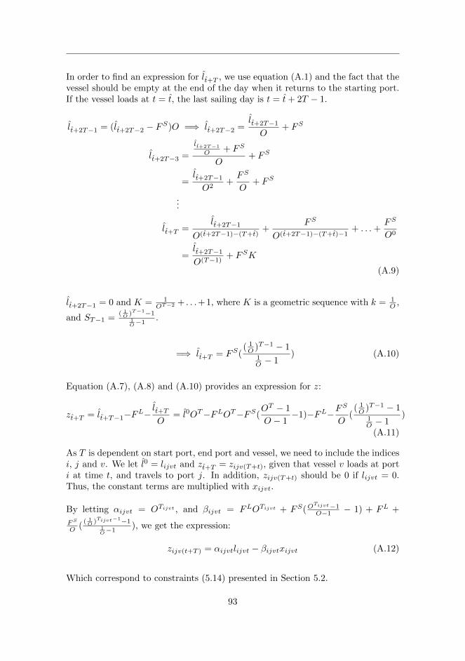
In order to find an expression for lt+T , we use equation (A.1) and the fact that thevessel should be empty at the end of the day when it returns to the starting port.If the vessel loads at t = t, the last sailing day is t = t+ 2T − 1.
lt+2T−1 = (lt+2T−2 − FS)O =⇒ lt+2T−2 =
lt+2T−1O
+ FS
lt+2T−3 =
lt+2T−1
O + FS
O+ FS
=lt+2T−1O2
+FS
O+ FS
...
lt+T =lt+2T−1
O(t+2T−1)−(T+t)+
FS
O(t+2T−1)−(T+t)−1+ . . .+
FS
O0
=lt+2T−1O(T−1) + FSK
(A.9)
lt+2T−1 = 0 and K = 1OT−2 + . . .+1, where K is a geometric sequence with k = 1
O ,
and ST−1 =( 1O )T−1−1
1O−1
.
=⇒ lt+T = FS(( 1O )T−1 − 1
1O − 1
) (A.10)
Equation (A.7), (A.8) and (A.10) provides an expression for z:
zt+T = lt+T−1−FL−
lt+TO
= l0OT−FLOT−FS(OT − 1
O − 1−1)−FL−F
S
O(( 1O )T−1 − 1
1O − 1
)
(A.11)
As T is dependent on start port, end port and vessel, we need to include the indicesi, j and v. We let l0 = lijvt and zt+T = zijv(T+t), given that vessel v loads at porti at time t, and travels to port j. In addition, zijv(T+t) should be 0 if lijvt = 0.Thus, the constant terms are multiplied with xijvt.
By letting αijvt = OTijvt , and βijvt = FLOTijvt + FS(OTijvt−1O−1 − 1) + FL +
FS
O (( 1O )Tijvt−1−1
1O−1
), we get the expression:
zijv(t+T ) = αijvtlijvt − βijvtxijvt (A.12)
Which correspond to constraints (5.14) presented in Section 5.2.
93

APPENDIX A. DERIVATION OF BOIL-OFF CONSTRAINTS
94

Appendix B
Graphs Showing MonthlyOver- and Under-deliveries
B.1 RHH Full Case
Figure B.1: Monthly deviations full case
95

APPENDIX B. GRAPHS SHOWING MONTHLY OVER- ANDUNDER-DELIVERIES
B.2 Aggregated Case
Aggregation Strategy 1
Figure B.2: Monthly deviations Strategy 1
Aggregation Strategy 2
Figure B.3: Monthly deviations Strategy 2
96

B.3. E-ADH AFTER POST-PROCESSING
Aggregation Strategy 3
Figure B.4: Monthly deviations Strategy 3
B.3 E-ADH After Post-processing
Figure B.5: Monthly deviations E-ADH after post-processing
97

APPENDIX B. GRAPHS SHOWING MONTHLY OVER- ANDUNDER-DELIVERIES
B.4 RHH-ADH After Post-processing
Figure B.6: Monthly deviations RHH-ADH after post-processing
98