a hands-on training session on matlab for signal...

FDP on Electronic Design Tools - MATLAB for Signal Processing 13/12/2017

Dr. A. Ranjith Ram – [email protected] 1

Resource Person : Dr. A. Ranjith RamAssociate Professor, ECE Dept.

Govt. College of Engineering KannurCell : 94476 37667

e-mail : [email protected]

Objectives : Study of Signals, Systems and Transforms

Design of FIR and IIR Filters

Advanced tools for Signal Processing

A Hands-on Training Session on

MATLAB for Signal ProcessingIn Connection with the FDP on Electronic Design Tools @ GCE Kannur

11th – 15th December 2017

Study of Signals, Systems and Transforms

30 Minutes


30 Minutes

Advanced tools for Signal Processing

30 Minutes

13 December 2017 2MATLAB for Signal Processing



Outline

Signals in MATLAB Environment

Correlation & Convolution

Laplace Transform & Z-Transform

Circular Convolution and Parseval’s Theorem

Systems – Impulse Response & Frequency Response

Transfer Function and Pole-Zero Plots


Advanced Tools : wvtool, fvtool, fdatool and sptool


ECE – Toolboxes of Interest

Signal Processing Toolbox

Communications System Toolbox

Computer Vision System Toolbox

DSP System Toolbox

Wavelet Toolbox

Image Acquisition Toolbox

Image Processing Toolbox

Data Acquisition Toolbox


Fuzzy Logic Toolbox

Symbolic Math Toolbox

Statistics Toolbox

Phased Array System Toolbox

Neural Network Toolbox

Optimization Toolbox

RF Toolbox

Control System Toolbox



Useful Built-in Functions exp()

dirac()

sinc()

erf()

erfc()

gamma()

xcorr()

corr()

laplace()

ztrans()

fft()

dct()

hilbert()


filter()

conv()

cconv()

impz

step()

freqz()

fir1()

firpm()

butter()

buttord()

cheby1()

cheby2()

sptool()

Signal Input to MALAB Three methods of inputting signals to MATLAB :

generated by using MATLAB functions itself

from memory

read an audio file

read a speech file

from I/O devices

input from a sensor

input from an instrument

Input from a microphone




Signal Input – Examples

x = rand(1, 200);

[x fs] = wavread(‘aud.wav’);

S = load(‘filemname’);

import menu – import a file


Signal Output from MATLAB

Three methods of outputting signals from MATLAB :

directly showing in the command window

to memory

create and write an audio file from a MATLAB variable

write an array of samples from a MATLAB variable

to I/O devices

output to a DAC

output to a loudspeaker

output to a display




Signal Output – Examples

sprintf(‘The signal is %d', x) or display(x)

fid = fopen('exp.txt','w');

fprintf(fid,'%6.2f %12.8f\n',y);

fclose(fid);

wavwrite(s,fs,‘au.wav’)

save(‘filename’, var)

save menu


/ sound(s,fs)

Generating Basic Analog Signals


>> t = 1:20;

>> a = 0.2;

>> x = exp(a*t);

>> plot(x);

Define the time span

Define other parameters

Generate the signal and plot it

Generate & plot an analog signum function

Generate & plot an analog sinc function

Generate & plot an analog gaussian function



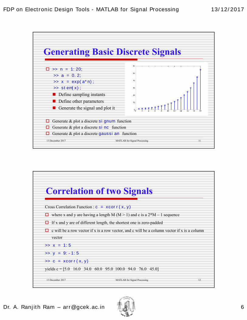
Generating Basic Discrete Signals


>> n = 1:20;

>> a = 0.2;

>> x = exp(a*n);

>> stem(x);

Define sampling instants

Define other parameters

Generate the signal and plot it

Generate & plot a discrete signum function

Generate & plot a discrete sinc function

Generate & plot a discrete gaussian function

Correlation of two Signals


Cross Correlation Function : c = xcorr(x,y)

where x and y are having a length M (M > 1) and c is a 2*M – 1 sequence

If x and y are of different length, the shortest one is zero-padded

c will be a row vector if x is a row vector, and c will be a column vector if x is a column

vector

>> x = 1:5

>> y = 9:-1:5

>> c = xcorr(x,y)

yields c = [5.0 16.0 34.0 60.0 95.0 100.0 94.0 76.0 45.0]



Autocorrelation function


ACF is given by c = xcorr(x), where x is a vector

when x is an M x N matrix, is a large matrix with 2*M – 1 rows whose N^2 columns

contain the cross-correlation sequences for all combinations of the columns of x

The zeroth lag of the output correlation is in the middle of the sequence, at element or

row M

>> x = 1:5

>> c = xcorr(x)

yields c = [5.0 14.0 26.0 40.0 55.0 40.0 26.0 14.0 5.0 ]

Convolution of two Signals


Convolution and polynomial multiplication : conv(x,y)

c = conv(x, y) convolves vectors x and y

c is a vector of length length(x) + length(y) – 1

If x and y are vectors of polynomial coefficients, convolving them is equivalent to

multiplying the two polynomials

>> x = 1:5

>> y = 9:-1:5

>> c = conv(x,y)

yields c = [9 26 50 80 115 96 74 50 25]



Transforms – Laplace & Z


The Laplace Transform gives the representation of a continuous time signal/system in

s domain

The Z Transform gives the representation of a discrete signal/system in z domain

One can say that t is transformed to s and n is transformed to z. Both s & z are

complex variables

Both needs no numerical computation, but an integration/summation of a

signal/sequence

To cope with such a situation, MATLAB supports another type of variable – the

symbolic variable

The Symbolic Math Toolbox


In MATLAB, symbolic variables are also possible, which do not possess any values,

but only symbolic in nature

Symbolic Math Toolbox provides functions for solving and manipulating symbolic

math expressions and performing variable-precision arithmetic

One can analytically perform differentiation, integration, simplification, transforms,

and equation solving. Also, one can generate code for MATLAB and Simulink from

symbolic math expressions.

>> syms x

>> diff(sin(x^2))

>> ans = 2*x*cos(x^2)



Laplace Transform


Laplace Transform : laplace(); Inverse LT : ilaplace()

>> syms t n

>> f = t^2;

>> disp(f);

>> F = laplace(f);

>> disp(F);

>> disp('Inverse Laplace transform is')

>> f1 = ilaplace(F);

>> disp(f1);

Z-Transform


Z-Transform : ztrans(); Inverse ZT : iztrans()

>> x = 0.5^n;

>> disp(x);

>> X = ztrans(x);

>> disp(X);

>> disp('Inverse Z-Transform is');

>> x1 = iztrans(X);

>> disp(x1);



Discrete Fourier Transform


Discrete (Fast) Fourier Transform : fft(); Inverse DFT : ifft()

fft(x) is the discrete Fourier transform (DFT) of vector x

For matrices, the fft operation is applied to each column

fft(x, N) is the N-point FFT, padded with zeros if x has less than N points and

truncated if it has more.

>> n = 1:50;

>> x = cos((pi/8)*n) + cos((pi/20)*n); plot(x)

>> X = fft(x); stem(abs(X))

>> xcap = ifft(X); plot(xcap)

Circular Convolution


Modulo-N circular convolution : cconv()

c = cconv(x, y, N) circularly convolves vectors x and y.

c is of length N. If omitted, N defaults to length(x) + length(y) – 1

When N = length(x) + length(y) – 1, the circular convolution is equivalent to the linear

convolution computed by conv()

>> a = [1 2 -1 1];

>> b = [1 1 2 1 2 2 1 1];

>> c = cconv(a,b,11)

>> cref = conv(a,b)



Parseval’s Theorem


The energy of a signal/sequence is a constant, irrespective of the domain

Steps:

Find out the energy in time domain

Transform the signal to frequency domain

Find out the energy of the spectra

Both values should be the same

>> x = [2 1 -2 3 4 -3 1 2];

>> e = sum(x.^2); % Energy from samples

>> X = fft(x);

>> E = sum(abs(X).^2)/8; % Energy from spectra

Discrete Time Systems – Impulse Response


Discrete Impulse Response : impz(b,a)

b : numerator vector; a : denominator vector

>> b=[0.0013 0.0064 0.0128 0.0128 0.0064 0.0013];

>> a=[1 -2.9754 3.8060 -2.5453 0.8811 -0.1254];

>> h = impz(b,a); % Impulse Response, h(n)

>> stem(h);

>> grid on;

>> title('Impulse Response');

>> ylabel('Response');

>> xlabel('n');



Systems – Transfer Function


>> sys = tf(b,a) creates a continuous-time transfer function SYS with numerator b

and denominator a.

>> sys = tf(b,a,TS) creates a discrete-time transfer function with sampling time

TS (set TS = -1 if the sampling time is undetermined).

>> b = [0.0013 0.0064 0.0128 0.0128 0.0064 0.0013];

>> a = [1 -2.9754 3.8060 -2.5453 0.8811 -0.1254];

>> sys = tf(b,a)

sys =

0.0013 s^5 + 0.0064 s^4 + 0.0128 s^3 + 0.0128 s^2 + 0.0064 s + 0.0013

s^5 - 2.975 s^4 + 3.806 s^3 - 2.545 s^2 + 0.8811 s - 0.1254

Systems – Frequency Response


[H,W] = freqz(b,a,N) returns the N-point complex frequency response vector

H and the N-point frequency vector W in radians/sample of the digital system

>> b = [0.0013 0.0064 0.0128 0.0128 0.0064 0.0013];

>> a = [1 -2.9754 3.8060 -2.5453 0.8811 -0.1254];

>> freqz(b,a)



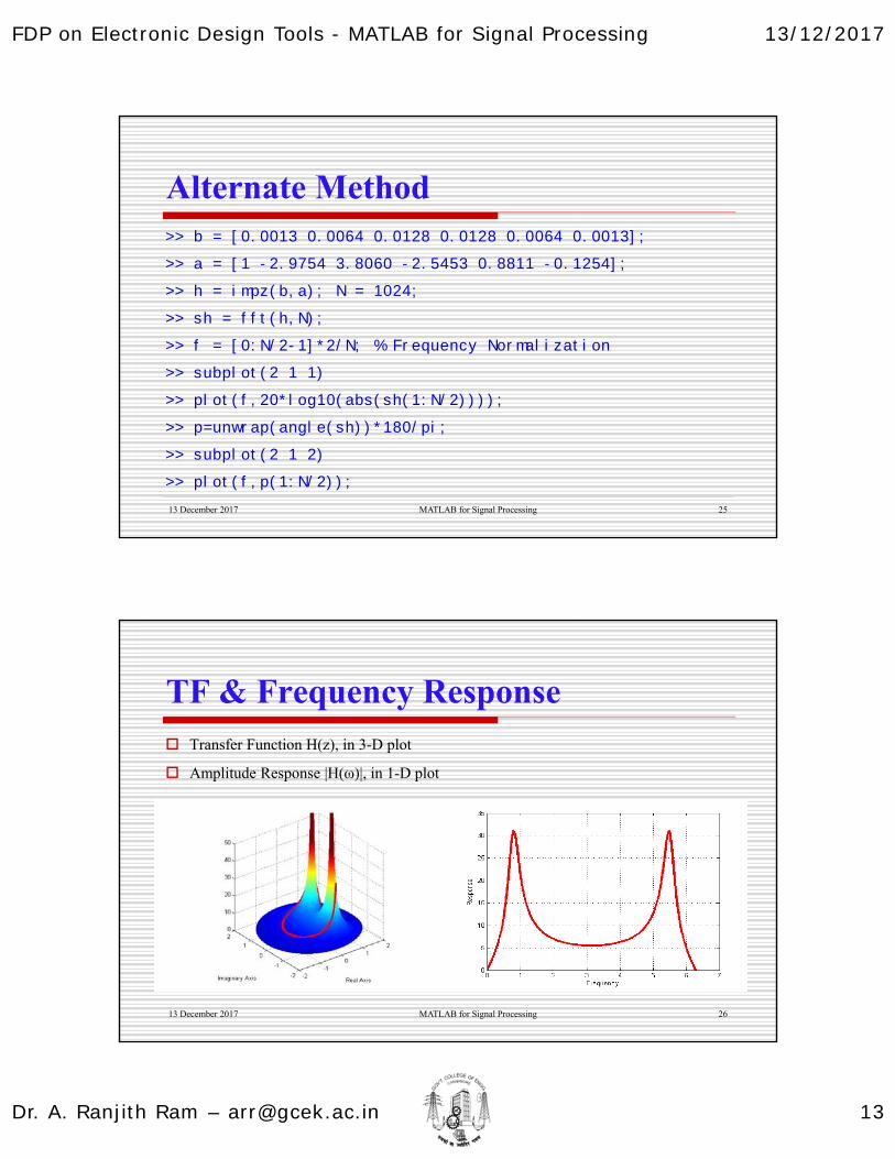
Alternate Method


>> b = [0.0013 0.0064 0.0128 0.0128 0.0064 0.0013];

>> a = [1 -2.9754 3.8060 -2.5453 0.8811 -0.1254];

>> h = impz(b,a); N = 1024;

>> sh = fft(h,N);

>> f = [0:N/2-1]*2/N; % Frequency Normalization

>> subplot(2 1 1)

>> plot(f,20*log10(abs(sh(1:N/2))));

>> p=unwrap(angle(sh))*180/pi;

>> subplot(2 1 2)

>> plot(f,p(1:N/2));

TF & Frequency Response


Transfer Function H(z), in 3-D plot

Amplitude Response |H(ω)|, in 1-D plot



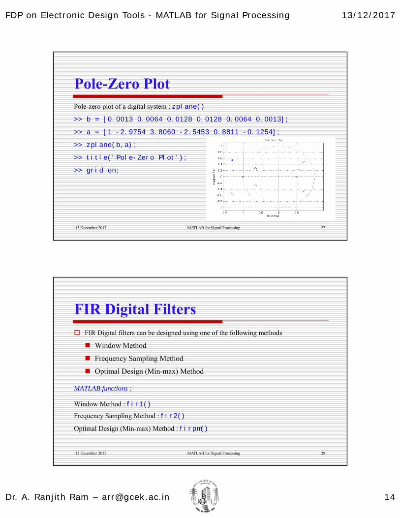
Pole-Zero Plot


Pole-zero plot of a digital system : zplane()

>> b = [0.0013 0.0064 0.0128 0.0128 0.0064 0.0013];

>> a = [1 -2.9754 3.8060 -2.5453 0.8811 -0.1254];

>> zplane(b,a);

>> title('Pole-Zero Plot');

>> grid on;

FIR Digital Filters


FIR Digital filters can be designed using one of the following methods

Window Method

Frequency Sampling Method

Optimal Design (Min-max) Method

MATLAB functions :

Window Method : fir1()

Frequency Sampling Method : fir2()

Optimal Design (Min-max) Method : firpm()



FIR Filter Design – Window Method


FIR filters are linear phase discrete time systems

Since the FIR systems are having bn’s only (an’s are zeros except a0), the task is in finding bn’s – the numerator coefficients

FIR filters can be designed classically by windowing technique

Here the impulse response of the ideal filter is windowed to get a finite duration sequence

If hd(n) is the impulse response of the desired (ideal) filter, the designed (actual) impulse response is given by h(n) = hd(n) . w(n) where w(n) is the window function

The transition band of the filter directly determines its order

The selection of the window is based on the minimum stop band attenuation required

FIR Filter Design – Window Method


b = fir1(N,wn) designs an N'th order lowpass FIR digital filter

It returns the filter coefficients in length N+1 vector b

The cut-off frequency wn must be between 0 < wn < 1.0, with 1.0 corresponding to half the sample rate

The filter b is real and has linear phase. The normalized gain of the filter at wn is –6 dB

b = fir1(N,wn,'high') designs an N'th order high-pass filter

If wn is a two-element vector, wn = [w1 w2], fir1 returns an order N band-pass filter with pass-band w1 < w < w2

One can also specify b = fir1(N,wn,'bandpass')

If wn = [w1 w2], b = fir1(N,wn,'stop') will design a band-stop filter



FIR Filter Design (Contd…)


b = fir1(N,wn,window) designs an N-th order FIR filter using the N+1 length

window vector of the impulse response

If empty or omitted, fir1 uses a Hamming window of length N+1

For a complete list of available windows, see the help for the window function

Kaiser and Chebwin can be specified with an optional trailing argument

For example, b = fir1(N,Wn,kaiser(N+1,4)) uses a Kaiser window with

beta = 4

b = fir1(N,wn,'high',chebwin(N+1,r)) uses a Chebyshev window with

r decibels of relative side-lobe attenuation

FIR Filter Design (Contd…)


For filters with a gain other than zero at fs/2, e.g., high-pass and band-stop filters, N

must be even. Otherwise, N will be incremented by one

In this case the window length should be specified as N+2

By default, the filter is scaled so the center of the first pass band has magnitude exactly

one after windowing

Use a trailing 'noscale' argument to prevent this scaling, e.g.,

b = fir1(N,Wn,'noscale')

b = fir1(N,Wn,'high','noscale')

b = fir1(N,Wn,wind,'noscale')

We can also specify the scaling explicitly, e.g. fir1(N,wn,'scale')



FIR Filter Design – example


% Design a 48th-order FIR band-pass filter with

% pass-band 0.35 <= w <= 0.65

b = fir1(48,[0.35 0.65]);

freqz(b,1,512)

If N (Order) is not Given ?


Mitra's book for Digital Signal Processing quotes Kaiser with a simple estimate

N = [-20 * log10 (sqrt (rp * rs)) - 13] / [14.6 (ws - wp) / 2π]

where rp and rs are the pass-band ripple peak and stop-band ripple peak values, ws and wp are the stop-band and pass-band edges (which are normalized to 2π, where 2π = fs).

So, N is a direct function of the ripple peaks and an inverse function of the normalized transition band width)

If rp and rs are both 0.01 and (ws - wp) / 2π = 0.1 then

N = [-20 * log10 (sqrt (10 ^ -4)) - 13] / [1.46]

= [-20 * -2 - 13] / 1.46

= 27/1.46 = 18.5 or, rounded up to 19.



Optimal Design of FIR Filters


Parks-McClellan optimal equi-ripple FIR filter design : firpm()

b = firpm(N,F,A) returns a length N+1 linear phase (real, symmetric

coefficients) FIR filter which has the best approximation to the desired frequency

response described by F and A in the mini-max sense

F is a vector of frequency band edges in pairs, in ascending order between 0 and 1

1 corresponds to the Nyquist frequency or half the sampling frequency

At least one frequency band must have a non-zero width

A is a real vector, the same size as F which specifies the desired amplitude of the

frequency response of the resultant filter B



The desired response is the line connecting the points (F(k), A(k)) and (F(k+1), A(k+1))

for odd k; firpm treats the bands between F(k+1) and F(k+2) for odd k as transition

bands or don't care regions

Thus the desired amplitude is piecewise linear with transition bands

The maximum error is minimized.

For filters with a gain other than zero at fs/2, e.g., high-pass and band-stop filters, N

must be even. Otherwise, N will be incremented by one

Alternatively, you can use a trailing 'h' flag to design a type 4 linear phase filter and

avoid incrementing N.

b = firpm(N,F,A,W) uses the weights in W to weight the error





>> % Example of a length 31 low-pass filter

>> h=firpm(30,[0 .1 .2 .5]*2,[1 1 0 0]);

>> freqz(h,1,512)

gives the frequency response :

IIR Filters


IIR systems are not having any linear phase property

Occur as having recursive structures

Since the IIR systems are having both an’s and bn’s, the task is in finding both of the numerator and denominator coefficients

Classical analog filter design theory could be used for designing IIR filters

Hence there are many approximations – Butterworth, Chebyshev, Elliptical, etc.

Butterworth approximation is having a smooth passband as well as a stopband

But a Chebyshev approximation is either the passband having a ripple (Type-I) or the stopband having a ripple (Type-II)



IIR Filters – Transfer Function


Zero-pole-gain to second-order sections model conversion : zp2sos()

[sos, g] = zp2sos(z,p,k) finds a matrix sos in second-order sections form

and a gain g which represent the same system H(z) as the one with zeros in vector z,

poles in vector p and gain in scalar k

The poles and zeros must be in complex conjugate pairs

sos is an L by 6 matrix with the following structure :

[b01 b11 b21 1 a11 a21

b02 b12 b22 1 a12 a22

...

b0L b1L b2L 1 a1L a2L]

IIR Transfer Function (Contd…)


Each row of the sos matrix describes a 2nd order transfer function H(z) :

(b0k + b1k z^-1 + b2k z^-2)

(1 + a1k z^-1 + a2k z^-2) , where k is the row index.

g is a scalar which accounts for the overall gain of the system

If g is not specified, the gain is embedded in the first section

The second order structure thus describes the system H(z) as:

H(z) = g H1(z) H2(z) ... HL(z)

Embedding the gain in the first section when scaling a direct-form II structure is not

recommended and may result in erratic scaling. To avoid embedding the gain, use

zp2sos with two outputs.



IIR Transfer Function (Contd…)


Zero-pole to transfer function conversion : zp2tf()

[b,a] = zp2tf(z,p,k) forms the transfer function b(s)/a(s), given a set of zero

locations in vector z, a set of pole locations in vector p, and a gain in scalar k

Vectors b and a are returned with numerator and denominator coefficients in

descending powers of s.

Zero-pole to state-space conversion : zp2ss()

[A,B,C,D] = zp2ss(z,p,k) calculates a state-space model

x = Ax + Bu

y = Cx + Du, the A,B,C,D matrices are returned in block diagonal form

IIR Filter Design – Butterworth


Butterworth digital and analog filter design : butter()

[b, a] = butter(N,wn) designs an Nth order lowpass Butterworth filter and

returns the filter coefficients in length N+1 vectors b and a

The coefficients are listed in descending powers of z. The cutoff frequency Wn must be

0 < wn < 1, with 1 corresponding to half the fs

If wn is a two-element vector, wn = [w1 w2], butter returns an order 2N bandpass

filter with passband w1 < w < w2

[b,a] = butter(N,Wn,'high') designs a highpass filter; [b,a] =

butter(N,Wn,'low') designs a lowpass filter and [b,a] =

butter(N,Wn,'stop') is a bandstop filter if wn = [w1 w2]



IIR Filter Design – butter & buttord


When used as [z,p,k] = butter(…), the zeros and poles are returned in length N

column vectors z and p, and the gain in scalar k

When used with four left-hand arguments, as in [A,B,C,D] = butter(...),

state-space matrices are returned

butter(N,wn,'high','s') designs an analog HP Butterworth filter. In this case,

wn is in [rad/s] and it can be > 1

Butterworth filter order selection : buttord()

[N, wn] = buttord(wp,ws,rp,rs) returns the order N of the lowest order

digital Butterworth filter which has a passband ripple of no more than rp dB and a

stopband attenuation of at least rs dB

IIR Filter Design – Buttord


wp and ws are the passband and stopband edge frequencies, normalized from 0 to 1

(where 1 corresponds to pi radians/sample). e.g., Lowpass: wp = 0.1, ws = 0.2 &

Bandstop: wp = [0.1 .8], ws = [0.2 0.7]

buttord also returns wn, the Butterworth natural frequency (or, the 3 dB frequency) to

use with butter to achieve the specifications

[N, wn] = buttord(wp, ws, rp, rs, 's') does the computation for an

analog filter, in which case wp and ws are in radians/second

When rp is chosen as 3 dB, the wn in butter is equal to wp in buttord



IIR Filter Design – Butterworth Example


>> % For data sampled at 1000 Hz, design a lowpass

>> % filter with less than 3 dB of ripple in the

>> % passband, defined from 0 to 40 Hz, and at least

>> % 60 dB of attenuation in the stopband, defined

>> % from 150 Hz to the Nyquist frequency (500 Hz)

>> Wp = 40/500;

>> Ws = 150/500;

>> [n,Wn] = buttord(Wp,Ws,3,60); % Gives the order

>> [b,a] = butter(n,Wn); % Butterworth filter design

>> freqz(b,a,512,1000);% Plots the frequency response

IIR Filter Design – Chebyshev


[N,wp] = cheb1ord(wp,ws,rp,rs) returns the order N of the lowest order

digital Chebyshev Type-I filter which has a passband ripple of no more than rp dB and a

stopband attenuation of at least rs dB

[b,a] = cheby1(N,r,wp) designs an Nth order lowpass digital Chebyshev filter

with r decibels of peak-to-peak ripple in the passband

[N,ws] = cheb2ord(wp,ws,rp,rs) returns the order N of the lowest order

digital Chebyshev Type-II filter which has a passband ripple of no more than rp dB and

a stopband attenuation of at least s dB

[b,a] = cheby2(N,r,wst) : Nth order LP digital Chebyshev filter with the

stopband ripple r dB down and stopband-edge frequency wst



1-D Filtering Process


One-dimensional digital filtering : filter()

y = filter(b,a,x) filters the data in vector x with the filter described by vectors

a and b to create the filtered data y

The filter is a Direct Form II Transposed implementation of the standard difference

equation, a(1)y(n) = b(1)x(n) + b(2)x(n-1) + ... + (nb+1)x(n-nb) – a(2)y(n-1) – ... –

a(na+1)y(n-na)

If a(1) is not equal to 1, filter normalizes the filter coefficients by a(1).

filter() always operates along the first non-singleton dimension, namely

dimension 1 for column vectors and non-trivial matrices, and dimension 2 for row

vectors

1-D Filtering Process – Example


>> wp=0.3; ws=0.4; rp=1; rs=10; % Specifications

>> [n,wn] = buttord(wp,ws,rp,rs); % Order selection

>> [b,a] = butter(n,wn); % IIR filter design

>> figure(1); freqz(b,a);

>> title('The frequency response of LP IIR filter');

>> t=1:100;

>> sig1 = sin(0.1*pi*t); % Signal inside the PB

>> sig2 = sin(0.6*pi*t); % Signal inside the SB

>> sig = sig1 + sig2;

>> filsig = filter(b,a,sig); figure(2); plot(filsig)




>> % Analysis of a single window

>> w = chebwin(64,100);

>> wvtool(w);

>> % Analysis of multiple vectors

>> w1 = bartlett(64);

>> w2 = hamming(64);

>> wvtool(w1,w2);

Window Visualization Tool – wvtool

Filter Visualization Tool – fvtool


[b,a] = butter(5, 0.5);

h1 = fvtool(b, a);



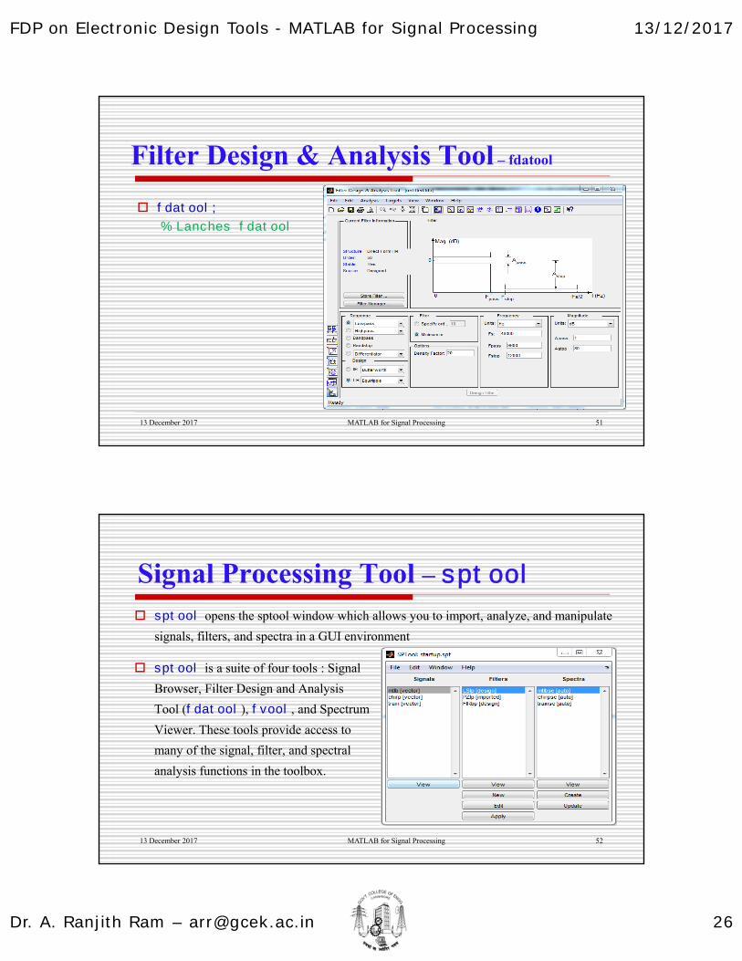
Filter Design & Analysis Tool – fdatool


fdatool;

% Lanches fdatool

Signal Processing Tool – sptool


sptool opens the sptool window which allows you to import, analyze, and manipulate

signals, filters, and spectra in a GUI environment

sptool is a suite of four tools : Signal

Browser, Filter Design and Analysis

Tool (fdatool), fvool, and Spectrum

Viewer. These tools provide access to

many of the signal, filter, and spectral

analysis functions in the toolbox.



Thanks

[email protected]


a hands-on training session on matlab for signal...

Documents