1

A Hands-On Introduction to SAS Programming Casey Cantrell, Clarion Consulting, Los Angeles, CA

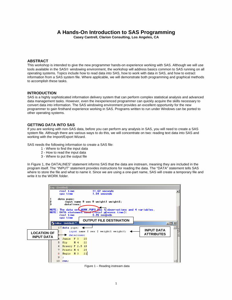
ABSTRACT This workshop is intended to give the new programmer hands-on experience working with SAS. Although we will use tools available in the SAS® windowing environment, the workshop will address basics common to SAS running on all operating systems. Topics include how to read data into SAS, how to work with data in SAS, and how to extract information from a SAS system file. Where applicable, we will demonstrate both programming and graphical methods to accomplish these tasks. INTRODUCTION SAS is a highly sophisticated information delivery system that can perform complex statistical analysis and advanced data management tasks. However, even the inexperienced programmer can quickly acquire the skills necessary to convert data into information. The SAS windowing environment provides an excellent opportunity for the new programmer to gain firsthand experience working in SAS. Programs written to run under Windows can be ported to other operating systems. GETTING DATA INTO SAS If you are working with non-SAS data, before you can perform any analysis in SAS, you will need to create a SAS system file. Although there are various ways to do this, we will concentrate on two: reading text data into SAS and working with the Import/Export Wizard. SAS needs the following information to create a SAS file: 1 - Where to find the input data 2 - How to read the input data 3 - Where to put the output file In Figure 1, the DATALINES” statement informs SAS that the data are instream, meaning they are included in the program itself. The “INPUT” statement provides instructions for reading the data. The “DATA” statement tells SAS where to store the file and what to name it. Since we are using a one-part name, SAS will create a temporary file and write it to the WORK folder.

Figure 1 – Reading instream data

LOCATION OF INPUT DATA

OUTPUT FILE DESTINATION

INPUT DATA ATTRIBUTES

2

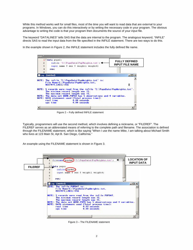
While this method works well for small files, most of the time you will want to read data that are external to your programs. In Windows, you can do this interactively or by writing the necessary code in your program. The obvious advantage to writing the code is that your program then documents the source of your input file. The keyword “DATALINES” tells SAS that the data are internal to the program. The analogous keyword, “INFILE” directs SAS to read the input data from the file specified in the INFILE statement. There are two ways to do this. In the example shown in Figure 2, the INFILE statement includes the fully defined file name.

Figure 2 – Fully defined INFILE statement

Typically, programmers will use the second method, which involves defining a nickname, or “FILEREF”. The FILEREF serves as an abbreviated means of referring to the complete path and filename. The association is defined through the FILENAME statement, which is like saying “When I use the name Mike, I am talking about Michael Smith who lives at 123 Main St, Apt B. San Diego, California.” An example using the FILENAME statement is shown in Figure 3.

Figure 3 – The FILENAME statement

FULLY DEFINED INPUT FILE NAME

LOCATION OF INPUT DATA

FILEREF

3

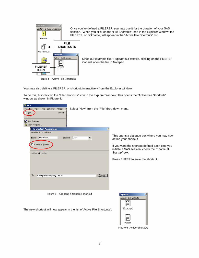
Once you’ve defined a FILEREF, you may use it for the duration of your SAS session. When you click on the “File Shortcuts” icon in the Explorer window, the FILEREF, or nickname, will appear in the “Active File Shortcuts” list.

Since our example file, “Pupdat” is a text file, clicking on the FILEREF icon will open the file in Notepad.

Figure 4 – Active File Shortcuts

You may also define a FILEREF, or shortcut, interactively from the Explorer window. To do this, first click on the “File Shortcuts” icon in the Explorer Window. This opens the “Active File Shortcuts” window as shown in Figure 4.

Select “New” from the “File” drop-down menu.

This opens a dialogue box where you may now define your shortcut.

If you want the shortcut defined each time you

initiate a SAS session, check the “Enable at Startup” box.

Press ENTER to save the shortcut.

Figure 5 – Creating a filename shortcut

The new shortcut will now appear in the list of Active File Shortcuts”.

Figure 6- Active Shortcuts

FILEREF ICON

FILE SHORTCUTS

4

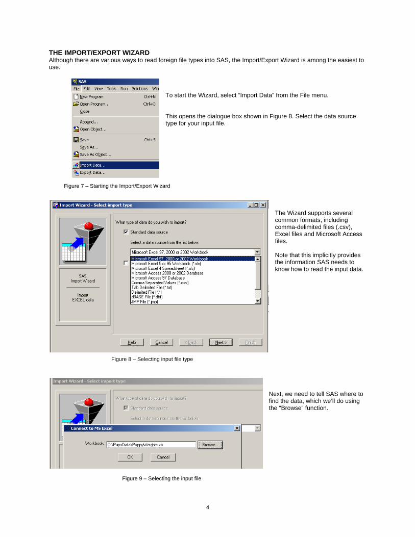
THE IMPORT/EXPORT WIZARD Although there are various ways to read foreign file types into SAS, the Import/Export Wizard is among the easiest to use. To start the Wizard, select “Import Data” from the File menu.

This opens the dialogue box shown in Figure 8. Select the data source type for your input file.

Figure 7 – Starting the Import/Export Wizard

The Wizard supports several common formats, including comma-delimited files (.csv), Excel files and Microsoft Access files. Note that this implicitly provides the information SAS needs to know how to read the input data.

Figure 8 – Selecting input file type

Next, we need to tell SAS where to find the data, which we’ll do using the “Browse” function.

Figure 9 – Selecting the input file

5

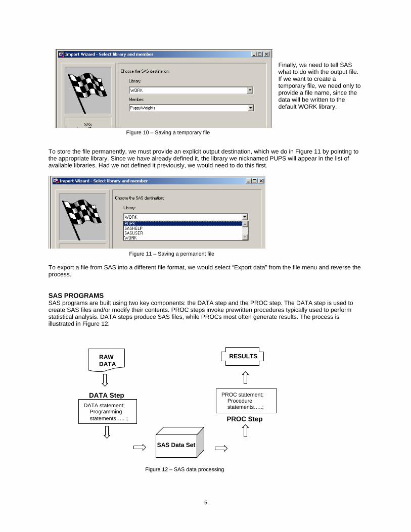
Finally, we need to tell SAS what to do with the output file. If we want to create a temporary file, we need only to provide a file name, since the data will be written to the default WORK library.

Figure 10 – Saving a temporary file

To store the file permanently, we must provide an explicit output destination, which we do in Figure 11 by pointing to the appropriate library. Since we have already defined it, the library we nicknamed PUPS will appear in the list of available libraries. Had we not defined it previously, we would need to do this first.

Figure 11 – Saving a permanent file To export a file from SAS into a different file format, we would select “Export data” from the file menu and reverse the process. SAS PROGRAMS SAS programs are built using two key components: the DATA step and the PROC step. The DATA step is used to create SAS files and/or modify their contents. PROC steps invoke prewritten procedures typically used to perform statistical analysis. DATA steps produce SAS files, while PROCs most often generate results. The process is illustrated in Figure 12.

Figure 12 – SAS data processing

RAW DATA

DATA statement; Programming statements….. ;

DATA Step

SAS Data Set

PROC statement; Procedure statements…..;

PROC Step

RESULTS

6

There are two important things to keep in mind. First, your data must be in SAS system file format before you can run any SAS procedures. Second, you may not mix DATA and PROC steps.

THE DATA STEP DATA steps are made up of programming statements, which may include assignment statements, conditional operations and/or subsetting operations. DATA steps always begin with the keyword DATA, followed by the name you want to give the file you are building. Remember that all SAS data files have two part names. If you want to create a permanent file you need to provide both the filename and the library name. Assignment statements assign values to new or existing variables. These values may be:

A constant The value of another variable The results of a mathematical expression

Conditional operations perform operations on:

Some, but not all, records Some, but not all, conditions IF condition is met THEN action

Subsetting operations:

Include only specific records in the output file IF condition is met THEN include record

SAS PROCEDURES SAS procedures begin with the keyword PROC followed by the name of the procedure and the name of the file you want to use in the procedure. Procedures may include options and/or optional statement specific to the procedure. Although there are myriad procedures in the SAS system, we will discuss the following five, which you are certain to use: PROC CONTENTS - Display information about file and its contents PROC PRINT - Print some or all records, some or all variables PROC SORT - Rearrange the order of records PROC UNIVARIATE- Generate descriptive statistics PROC FREQ - Generate frequency tables and cross-tabs For the next set of exercises, we will be working with a SAS system file named “CLASS” which is stored in the SASHELP library. The SASHELP library is automatically defined each time SAS is started. The two-part name for the file is then “SASHELP.CLASS”. PROC CONTENTS First, let’s examine the contents of the file. We can do this interactively using FSVIEW as previously discussed, or we can write a program to provide similar information by running PROC CONTENTS as shown in Figure 13.

Figure 13 – PROC CONTENTS

PROC NAME

SAS FILE NAME

7

PROC CONTENTS lists variables in the file in alphabetical order (Figure 14). We may request an additional list showing variables in the order they appear in the file by including the POSITION option in our program (Figure 15).

Figure 14 – PROC CONTENTS listing

Figure 15 – Using the POSITION option in PROC CONTENTS

Figure 16 – Variables listed in POSITION order

PROC PRINT While PROC CONTENTS provides information about the file, the PRINT procedure actually prints the data. The default action for PROC PRINT is to print every variable for every record in the file, plus an observation number. Figures 17 and 18 show a PROC PRINT program and the output it generates.

Figure 17 – PROC PRINT Figure 18 – PROC PRINT listing

POSITION OPTION

8

We can control both content and format of PROC PRINT output by using any of several optional statements. The program shown in Figure 19 suppresses the observation number and uses the variable NAME instead by using the ID statement.

Figure 19 – Using the ID statement in PROC PRINT To select which variables are printed, we will use the VAR statement. In Figure 20, we have elected to print only two variables: NAME and AGE. Figure 20 – Using the VAR statement in PROC PRINT PROC UNIVARIATE Since it is always a good idea to run exploratory analysis before working with a file, we’ll run PROC UNIVARIATE to get some additional information about our data. As seen in Figure 22, UNIVARIATE provides several basic statistics, including mean, mode, median, and standard deviation. When we run UNIVARIATE without any options or optional Figure 21 – The VAR statement in PROC UNIVARIATE statements, the procedure generates statistics for every numeric variable in the file. We may request statistics for specific variables by listing them in the VAR statement. An example is shown in Figure 21.

9

Figure 22 – Output from PROC UNIVARIATE CREATING NEW VARIABLES Now that we have an idea what our data set looks like, we are ready to work with the file. First, we’ll create some new variables. Since we are changing the data file, our program must include two statements: the DATA statement, which names the new file and specifies its output destination, and the SET statement, which names the SAS input data set and indicates its location. The SET statement also provides implicit instructions about how to read the data, since SET is the keyword that tells SAS we are reading an existing SAS data set. Information about the data structure is already stored in the descriptor portion of the file. We need only to tell SAS where the file is stored. In the program below we are creating a new file named “students”. Since we have not given it a two part name, SAS will store it in the WORK library, and delete the file when we terminate the SAS session. Our input file is the existing SAS file named CLASS, found in the SASHELP library folder. We are adding three new variables to the file.

Figure 23 - Creating new variables in SAS

NEW OUTPUT

FILE

TEMPORARYINPUT SAS

FILE

CONSTANT

RESULT OF OPERATION

VALUE FROM EXISTING VARIABLE

10

SAVING YOUR PROGRAM Since there were no syntax errors in our program, let’s save it before we continue. Remember that we must explicitly save anything we want to keep since we are running interactively.

First, make sure the Program Editor is the active window, then select “Save as” from the “File” menu. This opens a dialogue box where you may browse to the desired destination folder.

Figure 24 – Saving a program

In this example, we will save the file in a folder called “ClassData”. Since the file is a SAS program, we will name it “Height.sas”. Click “Save” to complete the process.

Figure 25 – Saving a SAS program

Note that the program name now appears at the top of the Program Editor window.

Figure 26 – Program name shown in the Program Editor

11

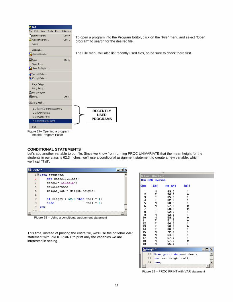
To open a program into the Program Editor, click on the “File” menu and select “Open program” to search for the desired file. The File menu will also list recently used files, so be sure to check there first.

Figure 27– Opening a program into the Program Editor CONDITIONAL STATEMENTS Let’s add another variable to our file. Since we know from running PROC UNIVARIATE that the mean height for the students in our class is 62.3 inches, we’ll use a conditional assignment statement to create a new variable, which we’ll call “Tall”.

Figure 28 – Using a conditional assignment statement This time, instead of printing the entire file, we’ll use the optional VAR statement with PROC PRINT to print only the variables we are interested in seeing.

Figure 29 – PROC PRINT with VAR statement

RECENTLY USED

PROGRAMS

12

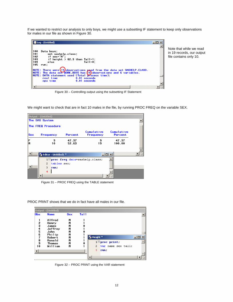
If we wanted to restrict our analysis to only boys, we might use a subsetting IF statement to keep only observations for males in our file as shown in Figure 30.

Note that while we read in 19 records, our output file contains only 10.

Figure 30 – Controlling output using the subsetting IF Statement

We might want to check that are in fact 10 males in the file, by running PROC FREQ on the variable SEX.

Figure 31 – PROC FREQ using the TABLE statement PROC PRINT shows that we do in fact have all males in our file.

Figure 32 – PROC PRINT using the VAR statement

13

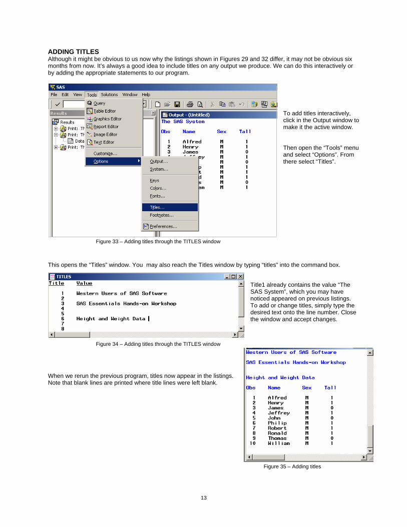
ADDING TITLES Although it might be obvious to us now why the listings shown in Figures 29 and 32 differ, it may not be obvious six months from now. It’s always a good idea to include titles on any output we produce. We can do this interactively or by adding the appropriate statements to our program.

To add titles interactively, click in the Output window to make it the active window. Then open the “Tools” menu and select “Options”. From there select “Titles”.

Figure 33 – Adding titles through the TITLES window

This opens the “Titles” window. You may also reach the Titles window by typing “titles” into the command box.

Title1 already contains the value “The SAS System”, which you may have noticed appeared on previous listings. To add or change titles, simply type the desired text onto the line number. Close the window and accept changes.

Figure 34 – Adding titles through the TITLES window When we rerun the previous program, titles now appear in the listings. Note that blank lines are printed where title lines were left blank.

Figure 35 – Adding titles

14

Titles entered using the “TITLES” window are global, meaning they remain in effect for the duration of the session and will appear in every listing. Since this may not be appropriate for every table, you may prefer to add titles statements to your program instead. The titles statement begins with the keyword TITLE followed by the appropriate line number, then the desired text enclosed in double quotation marks. Don’t forget the semi-colon!

TITLEn “Title for line number n “;

You may add up to 10 titles. In the example shown Figure 36, titles print on lines 1, 2 and 4, leaving a blank line since no title was specified for title 3.

Figure 36 – Writing TITLES statements

Note that when you change a TITLE (TITLEn), all titles which came after it (TITLE>n) will be cleared. PROC SORT The SORT procedure allows us to rearrange the order of records in the file based on values for the variables named in the BY statement.

PROC SORT DATA = filename; BY variable;

The program shown in Figure 37 sorts the file by Sex. Character variables are, of course, sorted alphabetically.

Figure 37 – PROC SORT

15

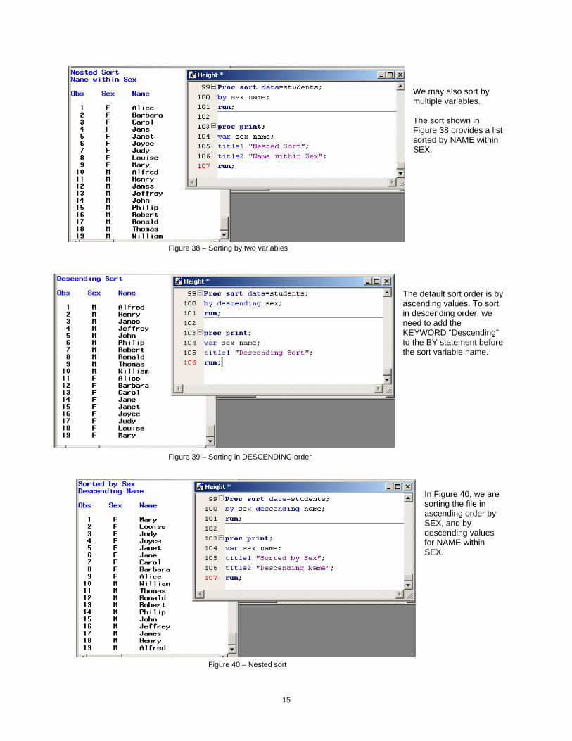
We may also sort by multiple variables. The sort shown in Figure 38 provides a list sorted by NAME within SEX.

Figure 38 – Sorting by two variables

The default sort order is by ascending values. To sort in descending order, we need to add the KEYWORD “Descending” to the BY statement before the sort variable name.

Figure 39 – Sorting in DESCENDING order

In Figure 40, we are sorting the file in ascending order by SEX, and by descending values for NAME within SEX.

Figure 40 – Nested sort

16

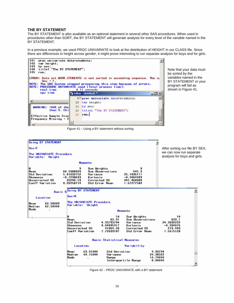
THE BY STATEMENT The BY STATEMENT is also available as an optional statement in several other SAS procedures. When used in procedures other than SORT, the BY STATEMENT will generate analysis for every level of the variable named in the BY STATEMENT. In a previous example, we used PROC UNIVARIATE to look at the distribution of HEIGHT in our CLASS file. Since there are differences in height across gender, it might prove interesting to run separate analysis for boys and for girls.

Note that your data must be sorted by the variables named in the BY STATEMENT or your program will fail as shown in Figure 41.

Figure 41 – Using a BY statement without sorting

After sorting our file BY SEX, we can now run separate analysis for boys and girls.

Figure 42 – PROC UNIVARIATE with a BY statement

17

PROC FREQ Although we have used PROC PRINT to look at our data, PROC FREQ will give us greater detail and more practical information. Although this procedure is typically used to generate frequency listings and cross tabulations, FREQ also generates useful statistics, such as chi-square values, odds ratios, and kappa coefficients. No preliminary analysis should be considered complete until we have looked at the distribution of variables by running PROC FREQ. Like PROC PRINT, when we run PROC FREQ without including any options or optional statements, we will get frequency listings for every variable in the file. To select specific tables, we will use the optional statement TABLES followed by the variable names. The TABLES statement is similar in this way to the VAR statement used in PRINT and UNIVARIATE. An example is shown in Figure 43.

Figure 43 – Simple frequencies

To generate cross tabs, we need only to insert an asterisk between the two variable names. In addition to simple frequencies, our listing includes column and row percentages as well.

Figure 44 – Cross tabulations using PROC FREQ

18

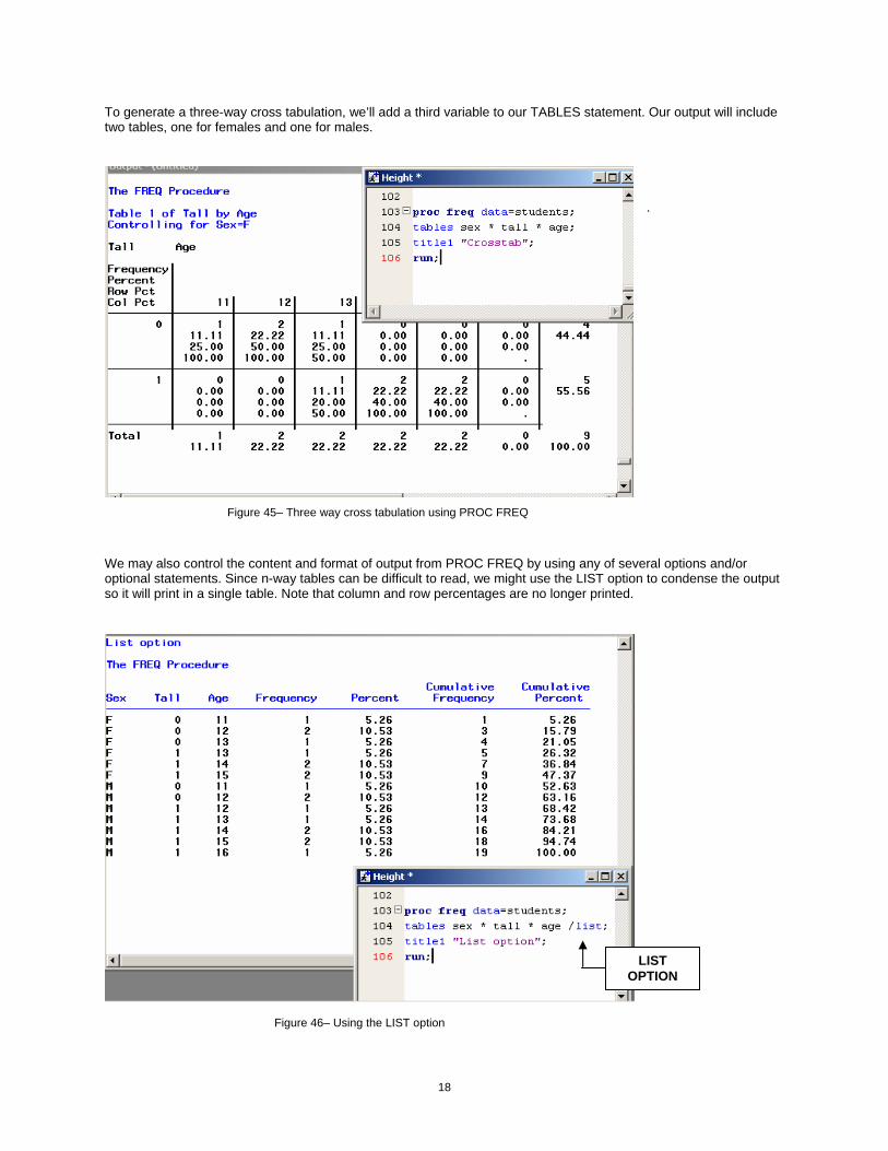
To generate a three-way cross tabulation, we’ll add a third variable to our TABLES statement. Our output will include two tables, one for females and one for males.

.

Figure 45– Three way cross tabulation using PROC FREQ We may also control the content and format of output from PROC FREQ by using any of several options and/or optional statements. Since n-way tables can be difficult to read, we might use the LIST option to condense the output so it will print in a single table. Note that column and row percentages are no longer printed.

Figure 46– Using the LIST option

LIST OPTION

19

Another alternative is to use the BY STATEMENT. Remember the BY STATEMENT will generate separate tables for each value of the variable named in the BY STATEMENT. The file must be sorted by the variables named in the BY statement.

Figure 47– Using the BY statement with PROC FREQ

By default, PROC FREQ does not print missing values. The MISSING option will add them to the table. In the example in Figure 48, one student has missing values for SEX and AGE, while another is missing SEX.

Figure 48– Using the MISSING option

MISSING OPTION

20

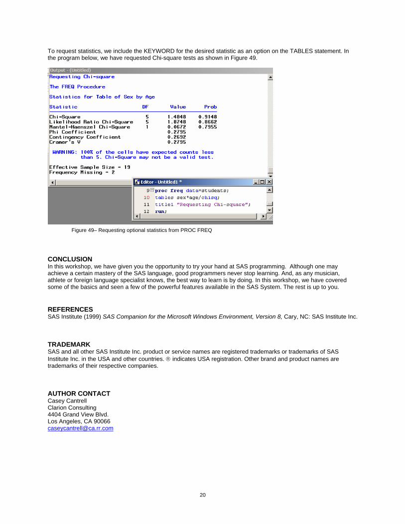
To request statistics, we include the KEYWORD for the desired statistic as an option on the TABLES statement. In the program below, we have requested Chi-square tests as shown in Figure 49.

Figure 49– Requesting optional statistics from PROC FREQ CONCLUSION In this workshop, we have given you the opportunity to try your hand at SAS programming. Although one may achieve a certain mastery of the SAS language, good programmers never stop learning. And, as any musician, athlete or foreign language specialist knows, the best way to learn is by doing. In this workshop, we have covered some of the basics and seen a few of the powerful features available in the SAS System. The rest is up to you. REFERENCES SAS Institute (1999) SAS Companion for the Microsoft Windows Environment, Version 8, Cary, NC: SAS Institute Inc.

TRADEMARK SAS and all other SAS Institute Inc. product or service names are registered trademarks or trademarks of SAS Institute Inc. in the USA and other countries. ® indicates USA registration. Other brand and product names are trademarks of their respective companies. AUTHOR CONTACT Casey Cantrell Clarion Consulting 4404 Grand View Blvd. Los Angeles, CA 90066 caseycantrell@ca.rr.com

21