a half-space problem in the theory of fractional order ...€¦ · space problem in the theory of ....

$: A half-space problem in the theory of fractional order ...€¦ · space problem in the theory of . fractional order thermoelasticity with diffusion. 1,2. Moustafa M. Salama, 1,3A.M$
International Journal of Scientific & Engineering Research, Volume 6, Issue 1, January-2015 358

ISSN 2229-5518

IJSER © 2015

http://www.ijser.org

A half-space problem in the theory of fractional order thermoelasticity with

diffusion. 1,2Moustafa M. Salama, 1,3A.M. Kozae, 1M. A. Elsafty,1,3S.S. Abelaziz

Abstract We consider in this work the problem of thermoelastic half-space with a permeating substance in contact

with the bounding plane by employing the fractional order theory of thermoelasticity, the bounding surface of the half -

space is taken to be traction free and subjected to a time dependent thermal shock. The chemical potential is also

assumed to be a known function of time on the bounding plane. for the inversion of the Laplace transform based on

Fourier expansion techniques. The temperature, displacement, stress, and concentration as well as the chemical

potential are obtained. Numerical computations are carried out and represented graphically.

Index Terms—Generalized thermoelasticity, Thermal shock, Thermoelastic diffusion, fractional order thermoelasticity,

diffusion.

—————————— ——————————

1. Introduction

Biot [1] developed the coupled theory of

thermoelasticity to deal with a defect of the uncoupled

theory that mechanical causes have no effect on the

temperature. However, this theory shares a defect of

the uncoupled theory in that it predicts infinite speeds

of propagation for heat waves.

Lord and Shulman [2] introduced the theory of

generalized thermoelasticity with one relaxation time

for the special case of an isotropic body. This theory

was extended by Dhaliwal and Sherief [3] to include

the anisotropic case. In this theory, a modified law of

heat conduction including both the heat flux and its

time derivative replaces the conventional Fourier’s

law. The heat equation associated with this theory is

hyperbolic and hence eliminates the paradox of

infinite speeds of propagation inherent in both the

uncoupled and coupled theories of thermoelasticity.

For this theory, Ignaczak [4] studied uniqueness of

solution; Sherief [5] proved uniqueness and stability.

Anwar and Sherief [6] and Sherief [7] developed the

state-space approach to this theory. Anwar and Sherief

[8] completed the integral equation formulation.

Sherief and Hamza [9, 10] solved some two-

dimensional problems and studied wave propagation.

Sherief and El-Maghraby [11, 12] solved two crack

problems. Sherief [13] solved thermoelastic half-space

with a permeating substance in contact with the

bounding plane in the context of the theory of

—————————————————————————————————— 1,2

Moustafa M. Salama, Math.

1Dept., Faculty of Science, Taif University 888, Saudi Arabia.

2Department of Computer-Based Engineering Applications,

Informatics Research Institute, City of Scientific Research and Technology Applications, Egypt, E-mail: [email protected] 1,

3 A.M. Kozae, Math. Dept., Faculty of Science, Tanta Uni., Tanta, Egypt, E-mail: [email protected] 1M. A. Elsafty , E-mail: [email protected]

IJSER

[email protected]


ISSN 2229-5518

IJSER © 2015


generalized thermoelastic diffusion with one

relaxation time.

El-Maghraby [14–16] solved some two-

dimensional problems for media affected by heat

sources and body forces.

Diffusion can be defined as the random walk, of an

ensemble of particles, from regions of high

concentration to regions of lower concentration. There

is now a great deal of interest in the

study of this phenomenon, due to its many

applications in geophysics and industrial applications.

In integrated circuit fabrication, diffusion is used to

introduce “dopants” in controlled amounts into the

semiconductor substrate. In particular, diffusion is

used to form the base and emitter in bipolar

transistors, form integrated resistors, and form the

source/drain regions in MOS transistors and dope

poly-silicon gates in MOS transistors. In most of these

applications, the concentration is calculated using

what is known as Fick’s law. This is a simple law that

does not take into consideration the mutual interaction

between the introduced substance and the medium into

which it is introduced or the effect of the temperature

on this interaction.

Nowacki [17–20] developed the theory of

thermoelastic diffusion. In this theory, the coupled

thermoelastic model is used. This implies infinite

speeds of propagation of thermoelastic waves.

Recently, Sherief et al. [21] developed the theory of

generalized thermoelastic diffusion that predicts finite

speeds of propagation for thermoelastic and diffusive

waves.

Fractional calculus has been used successfully to

modify many existing models of physical processes.

The first application of fractional derivatives was given

by Abel who applied fractional calculus in the solution

of an integral equation that arises in the formulation of

the tautochrone problem. One can state that the whole

theory of fractional derivatives and integrals was

established in the 2nd half of the 19th century. Caputo

and Mainardi [22-25] found good agreement with

experimental results when using fractional derivatives

for description of viscoelastic materials and established

the connection between fractional derivatives and the

theory of linear viscoelasticity. Right now there are

five different generalizations of the coupled theory of

thermoelasticity the details can be found in Hetnarski

and Ignaczak [26]. All five theories are based on

assumptions of one kind or another. Also, all these

theories model the problem of heat conductions in

solids as a purely wave propagation phenomenon.

Povstenko [13] made a review of thermoelasticity that

uses fractional heat conduction equation. The theory of

thermal stresses based on the heat conduction

equation with the Caputo time-fractional derivative is

used by Povstenko [27] to investigate thermal stresses

in an infinite body with a circular cylindrical hole.

Povstenko proposed and investigated new models that

use fractional derivative in [28,30]. Sherief et al. [31]

developed a new theory of thermoelasticity is derived

using the methodology of fractional calculus, proved a

uniqueness theorem and derived a reciprocity relation

and a variational principle. The theories of coupled

thermoelasticity and of generalized thermoelasticity

with one relaxation time follow as limit cases. A

uniqueness theorem for this model is proved. A

variational principle and a reciprocity theorem are

derived.

Sherief and Abd El-Latief [32]applied the fractional

order theory of thermoelasticity to a 2D problem for a

half-space.

2. Formulation of The Problem

We consider the problem of an isotropic

IJSER


ISSN 2229-5518

IJSER © 2015


thermoelastic half-space (x ≥ 0) with a permeating

substance (such as a gas) in contact with the upper

plane of the half-space (x = 0). The x-axis is taken

perpendicular to the upper plane pointing inwards.

This upper plane of the half-space is taken to be

traction free and is subjected to a time- dependent

thermal shock. The chemical potential is also

assumed to be a known function of time on the upper

plane. All considered functions are assumed to be

bounded and vanish as x → ∞.

The equation of motion in the absence of body

forces is given by [22]

i i , j j j ,i j , i , i1 2 = + ( + ) - - .u u u C

,

(1)

where ui are the components of the displacement

vector, T is the absolute temperature, C is the

concentration of the diffusive material in the elastic

body, λ, µ are Lamé’s constants, ρ is the density, and

β1 and β2 are the material constants given by

1 = (3+2) t and 2 = (3+2) c ,

t is the coefficient of linear thermal expansion, and

c is the coefficient of linear diffusion expansion.

The energy equation has the form [21] and it can

be written in fraction order as:

1 1 1

1 1 1

2

E 0 0 0 0 01k T =ρ +τ + T + τ + aT +τ ,βc

t t tt t t

T T e e C C

D

, (2)

where k is the thermal conductivity, 10 α , cE is

the specific heat at constant strain, τ0 is the thermal

relaxation time, ‘a’ is a measure of the

thermodiffusion effect, T0 is a reference temperature

assumed to obey the inequality 1T/)TT( 00

and eij are the components of the strain tensor given by

) u + u( 2

1 = e i, jj , iij . (3)

The diffusion equation has the form Sherief et al

(2004)

0 = C b D C + C + ,T a D + e D ii,iiiikk,2 , (4)

where D is the diffusion coefficient, b is a measure of

diffusive effect and is the diffusion relaxation time.

The constitutive equations have the form Sherief et al

(2004)

C )TT( e + e 2 = 201kkijijij ,

(5a)

)TT( a C b + e = P 0kk1

, (5b)

where ij are the components of the stress tensor and P is

the chemical potential.

It follows from the description of the problem

that all considered functions will depend on x and t only.

We thus obtain the displacement components of the

form,

ux = u(x,t) , uy = uz = 0 . (6)

The strain components are given by

x x y y zz xy yz zx = , = = = = = 0 e e e e e eDu

where x

=

D

The cubical dilatation e = ekk is equal to

. u = e D (7)

IJSER


ISSN 2229-5518

IJSER © 2015


From equation (5a), it follows that the stress tensor

components have the form

x x 1 2 = = ( + 2 ) u - - C , D (8a)

y y z z 1 2 = = u - - C , D (8b)

0 z xy zy x (9)

Equations (1), (2) and (4) thus reduce to

2

1 2 u = u + ( + ) e T C D D D D

,(10)

1 1 1

1 1 12

E 0 0 0 0 01k T =ρ +τ + T + τ + aT +τ ,βc

t t tt t t

T T e e C C

D

(11)

.0 = C b D C τ + C + Ta D+ e β D 222

2DDD

(12)

By using equation (7), equations (10) - (12) can be

written as

2

1 22

u = ( + 2 ) e - - ,

tT C

D D D

(13)

1 1 1

1 1 1

2

E 0 0 0 0 01k T =ρ +τ + T + τ + aT +τ ,βc

t t tt t t

T T e e C C

D

(14)

2

2 2 2

2 2

D e + D a + ( + - D b ) C = 0 .

t tT

D D D

(15)

The governing equations can be put in a more convenient

form by using the following non-dimensional variables

xcx η1* , ucu η1

* , tct ααη21* ,

0

2

1

*

0 τητ ααc , τητ αα21

* c ,

* 1 0( )

2

T T

,

2C 2*

C, *

2

PP

,

2

*

ijij ,

where /)2(c21 , k/cE .

Using the above non-dimensional variables

equations (13) - (15), take the following form where we

have dropped the asterisks for convenience

Cθuu 2 DDD , (16)

Cet∂

∂

t∂

∂11

1

0

2

D,

(17)

0CCCe 2

32

2

1

2 DDD ,

(18)

where

)(

2c

T

E

0

2

1

,

21

1

2a

)( ,

D

222

,

2

2

3

2b

)( .

Also equations (5b) and (8) take the form

Cexx

, (19a)

,C - ) 2

- 1 ( = = 2zz yy

e (19b)

13

eCP , (20)

where /)( 22 .

The initial conditions of the problem are taken to be

homogeneous while the boundary conditions are

, 0 = |) t ,x ( , 0 = |) t ,x (=x =x

uh (21)

IJSER


ISSN 2229-5518

IJSER © 2015


1 x = 0 x =

( x , t )( x , t ) = ( t ) , = 0 ,| |fh

x

(22)

2 x = x =

( x , t )P( x , t ) = ( t ) , = 0 ,| |fh

C

x

(23)

where f1(t) and f2(t) are known functions of t .

where f1(t) and f2(t) are known functions of t . This

means that the upper surface is traction free and acted

upon by two shocks.

2.1. SOLUTION IN THE LAPLACE

TRANSFORM DOMAIN

Introducing the Laplace transform defined by

the formula

dt f(t) e = (s)f ts

0

,

into equations (16)-(19) and (20) and using the

homogeneous initial conditions, we obtain

Cuus DDD 22

, (24)

Cess

1

1

0

2 D,(25)

02

3

2

2

2

1

2 Csse DDD ,

(26)

Ce

xx

, (27a)

y y z z 12

2 = = ( 1 - ) - C ,e

(27b)

3 1

P C e

.

(28)

Taking the divergence of equation (24), we obtain

2 2 22( ) e C = 0s D D D . (29)

Eliminating Cande between equations (25), (26) and

(29), we obtain

6 4 2

1 2 3( - + - ) = 0 .a a a D D D, (30)

where

s)s()(εα)(αεα)sτ(α

sa

323110

3

111121

1

,

)s(s)s)((εsαsε)sτ(α

sa

1111

1223

2

10

3

2

. -

) s( ) s( s = a

3

0

4

3

1

112

In a similar manner we can show that C and e satisfy

the equations

. 0 = ) a - a + a - ( 321 246 DDD,

(31)

6 4 2

1 2 3( - + - ) = 0 .a a a CD D D (32)

Equation (30) can be factorized as

2 2 22 2 2

1 2 3( - ) ( - ) ( - ) = 0 ,k k k D D D (33)

where 321 kandk,k are the roots with positive real

parts of the characteristic equation

0

3

2

2

4

1

6 akakak. (34)

IJSER


ISSN 2229-5518

IJSER © 2015


The solution of Eq. 33 has the form,

, e = ) s,x (3

1 = i

xk

iiA

, (35)

where Ai = Ai (s) are parameters depending on s

only.Similarly, the solution of Eqs. 31 and 32 can be

written as

e = )(x, '3

1 = i

xk

iiAse

, (36)

e = )(x, "3

1 = i

xk

iiAsC

, (37)

where Ai'' are parameters depending only on s.

Substituting from equations (35)-(37) into equations (25),

(26) and (29), we get

A ] s - k) ([ ) s + s(

)] s + s( ) ( k[ k =A i2

11

2

i0

02

2

i

2

i'

i

1

11

1

(38 )

2 1 2 14 2

i i 0 0"

i1 22

i0 1 1

- [ ( 1) (s + ) ] + ( + )s s s sk k = .

( s + ) [(1 ) - ]s ski

sA A

(39)

We thus have

ee] s - k) ([ ) s + s(

)] s + s( ) ( k[ k = ) s ,x (e xk

i

xk

i2

11

2

i0

02

2

i

2

i3

1 =i

ii B A

1

11

1

,

(40)

2 1 2 14 23

i i 0 0

1 22i = 1

i0 1 1

- [ ( 1) ( s + )] + ( + )s s s sk k( x ,s ) = e

( s + ) [(1 ) - ]s sk

ik x

i

sC A

.

(41)

Integrating both sides of equation (7) from x to infinity,

and assuming that u vanishes at infinity, we obtain upon

using the relation (40)

e ] )[( ) s + s (

)] s + s ( ) ( [ = s)(x,

3

1 = i

xki2

1

2

i11

0

101

2

ii iAsk1

1kku

. (42)

Substituting from equations (35), (40) and (41)

into equations (27a) and (28), we get

e ] )[(

)] s + s ( ) ( [

) + (= s)(x,

3

1 = i

xki2

1

2

i1

101

2

i

0

xxiA

sk1

1k

s1

s

(43)

e ] )[(

) s + ( s + ] ) s + s ( )( s [ k - k

) s + (

) s + (= s)(x, 00

22i

4i

3

1 = i

xki2

1

2

i1

121

0

2xx iA

sk1

s1

1

1P

.

(44)

In order to evaluate the unknown parameters A1, A2 and

A3, we shall use the Laplace transform of the boundary

conditions (21)-(23) together with equations (35), (43)

and (44). We thus arrive at the following set of linear

equations

0sk1

1kAi2

12i1

101

2i

] )[(

)] s + s ( ) ( [

3

1 = i ,

(45)

, ) s ( f= 1

3

1 = iAi

(46)

.

) + (

) s + () s (f =

] )[(k

] )s + (ss + ) ) s + (s 1) + ( + s ( k- k [

02

2i

0022

i4i

3

1 = i

s1

1

sk1

2

i2

1

2

i1

121

A

(47)

Solving the linear system of equations (45)-

(47), we can obtain the parameters A1-A3.This completes

the solution of the problem in the Laplace transform

domain.

INVERSION OF Laplace Transform

We shall now outline the numerical inversion

method used to find the solution in the physical

domain. Let )s,x(f be the Laplace transform of a function f(x, t). First, we use the inversion formula of the Laplace transform expression )s,x(f of the form[22]

IJSER


ISSN 2229-5518

IJSER © 2015


ic

ic

st ds)s,x(fei

)t,x(f2

1

where c is an arbitrary real number greater than all the

real parts of the singularities of (s)f . Taking s = c +

iy, the above integral takes the form

dyiycxfeπ

etxf ity

ct

),(2

),(

.

Expanding the function h(x,y,t) = exp(-ct)f(x, t) in a

Fourier series in the interval [0,2T], we obtain the

approximate formula [23]

DEtxftxf ),(),(,

where

20for ),(),(),(1

021 Tttxctxctxf

kk

,

(48)

and

,....2,1,0)],/,(Re[ / kTπikdxfe

T

dte

kc Ttπik

(49)

ED, the discretization error, can be made arbitrarily

small by choosing d large enough [15]. Since the

infinite series in equation (48) can only be summed up

to a finite number N of terms, the approximate value

of f(x, t) becomes

20for 1

021 Ttcc)t,x(f

N

kkN

(50)

Using the above formula to evaluate f(x, t), we

introduce a truncation error ET that must be added to

the discretization error to produce the total

approximation error.

Two methods are used to reduce the total

error. First, the “Korrecktur” method is used to reduce

the discretization error. Next, the -algorithm is used to

reduce the truncation error and hence to accelerate

convergence.

The Korrecktur method uses the following formula

to evaluate the function f(x, t) :

DcT EtTxfetxftxf

)2,(),(),( 2

,

where the discretization errors DD EE [23].

Thus, the approximate value of f(x, t) becomes

)2,(),(),( 2 tTxfetxftxf N

cTNNK

,(51)

N´ is an integer such that N´ < N.

We shall now describe the -algorithm that is

used to accelerate the convergence of the series in

equation (53). Let N=2q+1 where q is a natural

number, and let

m

1kkm cs

be the sequence of partial sums of equation (50). We

define the -sequence by

mm,1m,0 s,0

and

p+1,m = p-1,m+1 + 1/ (p,m+1-p,m) ,

p=1,2,3,...

It can be shown that [23], the sequence

1,1 , 3,1 , 5,1 , ... , N,1

converges to f( ,x t) + ED - c0/2 faster than the

sequence of partial sums

sm , m = 1,2,3,...

The actual procedure used to invert the Laplace

transforms consists of using equation (54) together

IJSER


ISSN 2229-5518

IJSER © 2015


with the -algorithm. The values of c and T are chosen according to the criteria outlined in [23].

3. NUMERICAL RESULTS

For the purpose of numerical illustration, the

problem was solved for the following choice of

the functions f1 (t ) and f2 (t ):

f1 (t ) = θ0 H (t ),

f2 (t ) = P0 H (t ),

where θ0 and P0 are constants and H (t ) is the

Heaviside unit step function.

We, thus, have

s

θ01 (s) f

s

P02 (s) f

The roots k1 , k2 , and k3 of the characteristic

equation are given by

]a + q sin p [23

111

k ,

] ) q sin cosq3p(-[a3

112

k,

] ) q sin cosq3p([a3

113

k

)3a-[(a 221p

,,

3

)(sin 1 rq

and

,2

27923

32131

p

aaaar

Copper material was chosen for purposes of

numerical evaluations. The material constants of

the problem are thus given by in SI units [24]

T0 = 293 K, ρ = 8,954 kg.m-3

, τ0 =0.0 2s, τ =0

.2s, cE = 383.1 J. kg -1

. K -1

, αt =1 .7 8× 10 -5

K-1

,

k = 386 W· m −1

· K-1

, λ =7 .7 6× 1010

kg · m -1

. s -2

, µ =3. 8 6×1010

kg · m -1

.s -2

, α c =1 .9 8× 10 -4

m 3. kg

-1, d =0.8 5× 10

-8 kg.s.m

-3, a =1.2×10

4

m2.s

-2.K

-1, b =0.9× 10

6 m 5· kg

-1. s

-2.

Using these values, it was found that

η = 8886.73, ε = 0.0168, β2 = 4, α1 = 5.43, α2 =

0.533, and α3 = 36.24.

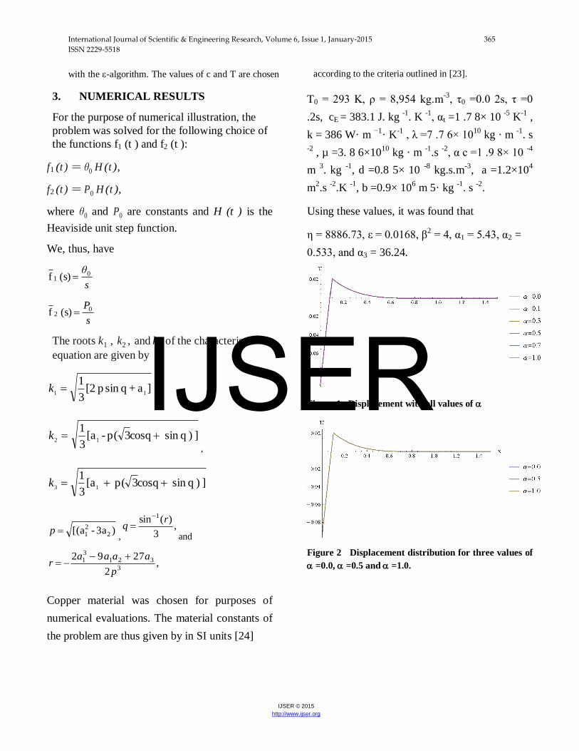
Figure 1 Displacement with all values of

Figure 2 Displacement distribution for three values of

=0.0, =0.5 and =1.0.

IJSER


ISSN 2229-5518

IJSER © 2015


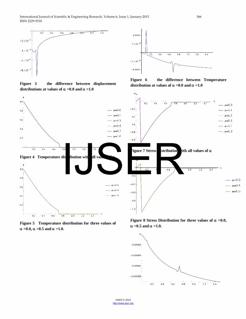
Figure 3 the difference between displacement

distributions at values of =0.0 and =1.0

Figure 4 Temperature distribution with all values of

Figure 5 Temperature distribution for three values of

=0.0, =0.5 and =1.0.

Figure 6 the difference between Temperature

distribution at values of =0.0 and =1.0

Figure 7 Stress Distribution with all values of

Figure 8 Stress Distribution for three values of =0.0,

=0.5 and =1.0.

IJSER


ISSN 2229-5518

IJSER © 2015


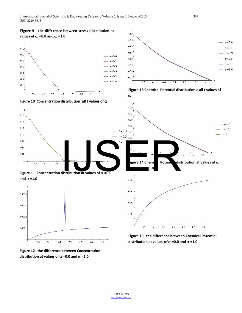
Figure 9 the difference between stress distribution at

values of =0.0 and =1.0

Figure 10 Concentration distribution all t values of

Figure 11 Concentration distribution at values of =0.0

and =1.0

Figure 12 the difference between Concentration


Figure 13 Chemical Potential distribution a all t values of

Figure 14 Chemical Potential distribution at values of

=0.0 and =1.0

Figure 15 the difference between Chemical Potential


IJSER


ISSN 2229-5518

IJSER © 2015


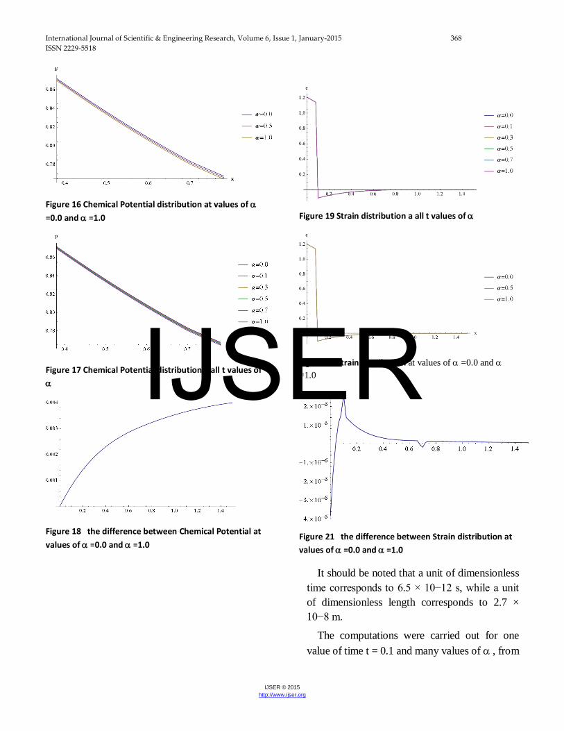
Figure 16 Chemical Potential distribution at values of

=0.0 and =1.0

Figure 17 Chemical Potential distribution a all t values of

Figure 18 the difference between Chemical Potential at


Figure 19 Strain distribution a all t values of

Figure 20 Strain distribution at values of =0.0 and

=1.0

Figure 21 the difference between Strain distribution at


It should be noted that a unit of dimensionless

time corresponds to 6.5 × 10−12 s, while a unit

of dimensionless length corresponds to 2.7 ×

10−8 m.

The computations were carried out for one

value of time t = 0.1 and many values of , from

IJSER


ISSN 2229-5518

IJSER © 2015


0.0 to 1.0 especially two values of alpha = 1

(corresponding to LordShulman theory) and =

0.5. The numerical method outlined above was

used to obtain the inverse Laplace transforms for

the temperature, displacement and stress

distributions. Fortran programming language

was used on a personal computer. The accuracy

maintained was 5 significant digits for both the

numerical integration and the inversion of the

Laplace transform.

The displacement, temperature, stress,

concentration, chemical potential, and strain are

shown in Figs. 1-3, 4-6, 7-9, 10-12, 13-18, and

19-21respectively.As expected from the order of

the partial differential equation, we have three

waves emanating from each surface; the fronts of

these waves are depicted in the figures as picks

in the functions .

We can see in all figures that, all the functions

considered have a non-zero value only in a

bounded region of space and vanish identically

outside this region. This region expands with the

passage of time. Also, our results are the sam as

As was mentioned by Sherief in [14] when =

1.0 , we here mentioned about the variation of

, from 0.0 to 1.0.

The displacement component u is shown in

Fig. 1, for all values of while fig. 2, show the

difference between displacements at =0.0 and

=1.0. It is clear that difference maintained was

7 significant digits, i.e the effect values of are

very weak, and we can see also in Fig.3 when,

we choose three values of ( = 0.0, = 0.5and

= 1), the same coclusions are in temperature is

shown in Figs. 4 to 6 , the stress component σxx

in Figs. 7 to 9, chemical Concentration Figs. 10

to 12, and strain Figs. 19 to 21. But we note that

in chemical potential Figs. 13 to 18 the effect

for values of maintained was 4 significant

digits only .

We can say that, for = 1 the solution is that

of the generalized theory of thermoelasticity and

exhibits the phenomenon of finite speeds of

propagation of waves. The question of whether

the solution for < 1 behaves similarly or not is

still an open question.

As was mentioned by Povstenko [17] ‘‘From

numerical calculations, it is difficult to say

whether the solution for a approaching 1 has a

jump at the wave front or it is continuous with

very fast changes. This aspect invites further

investigation’’. Our calculations show that up to

the specified accuracy, the solution seems to be

non-zero only in a finite region of space.

The problem was solved for many values of

< 1. The solutions seem to be of the same shape

as that of = 0.5 reported here. The difference is

that as a decreases the region where the solution

is non-zero becomes larger indicating faster

speed of propagation. It is known that for = 0,

the solution is that of the coupled theory of

thermoelasticity where the speed of propagation

of the waves is infinite.

4-Acknowledgment:

The Authors present their deeply thanks for

taif university for supporting us while doing in

this research.

5 -References

[1.] M. Biot, Thermoelasticity and irreversible thermo-dynamics. J. Appl. Phys. 27, 240 ,1956.

[2.] H. Lord, Y. Shulman, A generalized dynamical

theory of thermoelasticity, J. Mech. Phys. Solids 15 (1967) 299–309.H. Sherief, Ph.D. thesis,

University of Calgary, Canada, 1980

IJSER


ISSN 2229-5518

IJSER © 2015


[3.] R. Dhaliwal, H. Sherief, Generalized

thermoelasticity for anisotropic media.Q. Appl. Math. 33, 1 (1980)

[4.] J. Ignaczak, A Note on Uniqueness in

Thermoelasticity with One Relaxation Time, J.

Thermal Stresses, vol. 5, pp. 257-263, 1982.

[5.] H. Sherief, Sherief, On Uniqueness and Stability

in Generalized Thermoelasticity, Quart. Appl.

Math., vol.45, pp. 773- 778, 1987.

[6.] M. Anwar, H. Sherief, Sherief, State Space

Approach to Generalized Thermoelasticity, J.

ThermalStresses, vol. 11, pp. 353- 365, 1988.

[7.] H. Sherief, Sherief, State Space Formulation for

Generalized Thermoelasticity with One

Relaxation Time Including Heat Sources, J.

Thermal Stresses, vol. 16, pp. 163- 180, 1993.

[8.] M. Anwar, H. Sherief, Boundary integral

equation formulation of generalized

thermoelasticity in a Laplace transform domain, Appl. Math. Modell. 12 , 161–166,1988.

[9.] H. Sherief, F. Hamza, Hamza, Generalized

Thermoelastic Problem of a Thick Plate under Axisymmetric Temperature Distribution, J.

Thermal Stresses, vol. 17, pp. 435- 452, 1994.

[10.] H. Sherief, F. Hamza, Hamza, Generalized Two-

Dimensional Thermoelastic Problems in Spherical Regions under Axisymmetric

Distributions, J. Thermal Stresses, vol. 19, pp.

55- 76, 1996.

[11.] H. Sherief, N. El-Maghraby An internal penny

shaped-crack in an infinite thermoelastic solid, J.

Therm. Stress. vol.26 ,333–352, 2003

[12.] H. Sherief, N. El-Maghraby, A mode-I crack in an infinite space in generalized thermoelasticity,

J. Therm. Stress. Vol.28 ,465–484, 2005.

[13.] Hany H. Sherief and Heba A. Saleh, A Half-space Problem in the Theory of Generalized

Thermoelastic Diffusion, Int. J. Solids Struc.,

vol. 42, pp. 4484-4493, 2005.

[14.] N. El-MaghrabyA two-dimensional generalized

thermoelasticity problem for a half-space under

the action of a body force, J. Therm. Stress.

31557–568, ,2008.

[15.] N. El-Maghraby, A two-dimensional problem

for a thick plate with heat sources in generalized

thermoelasticity, J. Therm. Stress. vol.28 , 1227–

1241, 2005.

[16.] N. El-Maghraby, Two-dimensional problem in

generalized thermoelasticity with heat sources, J.

Therm. Stress. vol.27 , 227–240,2004.

[17.] W. Nowacki, “Dynamical problems of thermodiffusion in solids. Part I”,Bull. Pol.

Acad. Sci., Ser. IV (Techn. Sci.),22, 55–64,1974

[18.] W. Nowacki, Dynamical problems of thermodiffusion in solids II, Bull. Acad. Pol.

Sci., Ser. Sci. Tech. 22, 129–135,1974.

[19.] W. Nowacki, Dynamical problems of thermodiffusion in solids III, Bull. Acad. Pol.

Sci., Ser. Sci. Tech. 22 ,257–266, 1974.

[20.] W. Nowacki, Dynamical problems of

thermodiffusion in elastic solids, Proc. Vib. Prob. 15 ,105–128, 1974.

[21.] H. Sherief, F. Hamza, H. Saleh, The theory

of generalized thermoelastic diffusion, Int. J. Eng. Sci. 42, 591-608,2004.

[22.] Caputo, M., Linear model of dissipation whose

Q is almost frequency independent-II. Geophysical Journal of the Royal Astronomical

Society 13, 529-935, 1967.

[23.] Caputo, M., Vibrations on an infinite

viscoelastic layer with a dissipative memory. Journal of the Acoustical Society of America 56,

897–904, 1974.

[24.] Caputo, M., Mainardi, F., a. A new dissipation model based on memorymechanism. Pure and

Applied Geophysics 91, 134–147, 1971.

[25.] Caputo, M., Mainardi, F., b. Linear model of

dissipation in anelastic solids. Rivista del Nuovo cimento 1, 161–198, 1971.

[26.] Hetnarski, R.B., Ignaczak, J., Generalized

Thermoelasticity. Journal of Thermal Stresses 22, 4–5, 1999.

[27.] Y. Povstenko, Thermoelasticity that uses

fractional heat conduction equation, J. Math. Sci. 162 296–305,2009.

[28.] Y. Povstenko, Fractional radial heat conduction

in an infinite medium with a cylindrical cavity

and associated thermal stresses, Mech. Res. Commun. 37(2010) 436–440.

IJSER


ISSN 2229-5518

IJSER © 2015


[29.] Y. Povstenko, Fractional heat conduction and

associated thermal stress, J. Therm. Stresses 28 (2005) 83–102.

[30.] Y. Povstenko, Fractional Cattaneo-type

equations and generalized thermoelasticity, J.

Therm. Stresses 34 (2011) 97–114.

[31.] H.H. Sherief, A. El-Sayed, A.A. El-Latief,

Fractional order theory of thermoelasticity, Int. J.

Solids Struct. 47 (2010) 269–275.

[32.] Application of fractional order theory of

thermoelasticity to a 2D problem for a half-

space.

[33.]

IJSER

a half-space problem in the theory of fractional order ...€¦ · space problem in the theory of ....

Documents