A Graph-Based Semi-Supervised k Nearest-Neighbor

Method for Nonlinear Manifold Distributed Data

Classification

Enmei Tua,∗, Yaqian Zhangb, Lin Zhuc, Jie Yangd, Nikola Kasabove

aRolls-Royce@NTU Corporate Lab, Nanyang Technological University, SingaporebSchool of Computing Engineering, Nanyang Technological University, Singapore

cSchool of Computer Science and Technology, Shanghai University of Electric Power,China

dInstitute of Image Processing and Pattern Recognition, Shanghai Jiao Tong University,China

eThe Knowledge Engineering and Discovery Research Institute, Auckland University ofTechnology, New Zealand

Abstract

k Nearest Neighbors (kNN) is one of the most widely used supervised learningalgorithms to classify Gaussian distributed data, but it does not achieve goodresults when it is applied to nonlinear manifold distributed data, especiallywhen a very limited amount of labeled samples are available. In this paper,we propose a new graph-based kNN algorithm which can effectively handleboth Gaussian distributed data and nonlinear manifold distributed data.To achieve this goal, we first propose a constrained Tired Random Walk(TRW) by constructing an R-level nearest-neighbor strengthened tree overthe graph, and then compute a TRW matrix for similarity measurementpurposes. After this, the nearest neighbors are identified according to theTRW matrix and the class label of a query point is determined by the sum ofall the TRW weights of its nearest neighbors. To deal with online situations,we also propose a new algorithm to handle sequential samples based a localneighborhood reconstruction. Comparison experiments are conducted onboth synthetic data sets and real-world data sets to demonstrate the validityof the proposed new kNN algorithm and its improvements to other versionof kNN algorithms. Given the widespread appearance of manifold structures

∗Corresponding author: Enmei Tu, hellotem@hotmail.com

Preprint submitted to Elsevier June 6, 2016

arX

iv:1

606.

0098

5v1

[cs

.LG

] 3

Jun

201

6

in real-world problems and the popularity of the traditional kNN algorithm,the proposed manifold version kNN shows promising potential for classifyingmanifold-distributed data.

Keywords:k Nearest Neighbors, Manifold Classification, Constrained Tired RandomWalk, Semi-Supervised Learning

1. Introduction

k Nearest Neighbors (kNN) [9, 37, 52, 53] is one of the most popularclassification algorithms and has been widely used in many fields, such asintrusion detection [27], gene classification [26], semiconductor fault detec-tion [18], very large database manipulation [23], nuclear magnetic resonancespectral interpretation [24] and the prediction of basal area diameter [31],because it is simple but effective, and can generally obtain good results inmany tasks. One main drawback of the traditional kNN is that it does nottake the manifold distribution information into account and this can causebias which results in bad performance. It becomes even worse when thereare only a very small amount of labeled samples available. To address this,an example is shown in figure 1(a), in which there are two one-dimensionalmanifolds (the outer arch and the interior reflected S ) which correspond totwo classes, respectively. Each class has only 3 labeled samples, indicated bythe colored triangles and circles. Black dots are unlabeled samples. Figure1(b) - (d) show the 1NN, 2NN and 3NN classification results produced by thetraditional kNN, respectively. We can see that although the data have ap-parent manifold distribution, the traditional kNN incorrectly classifies manysamples due to ignoring the manifold information.

2

(a) Toy manifold data set (b) k=1

(c) k=2 (d) k=3

Figure 1: Results of traditional kNN classification with k=1, 2, 3 on manifold distributeddata, in which the colored shapes (red triangles and green dots) are labeled samples andthe black dots are unlabeled samples.

To improve the performance of the traditional kNN, some new kNN algo-rithms have been proposed. Hastie et. al. [17] proposed an adaptive kNN al-gorithm which computes a local metric for each sample and uses Mahalanobisdistance to find the nearest neighbors of a query point. Hechenbichler andSchliep [19] introduced a weight scheme to attach different importance tothe nearest neighbors with respect to their distances to the query point. Toreduce the effect of unbalanced training set sizes of different classes, Tan [39]used different weights for different classes regarding the number of labeledsamples in each class. There are also some other improvements and weightschemes for different tasks [8, 10, 12, 16, 25, 32, 51].

However, none of these new kNN algorithms takes manifold structureinto consideration explicitly. For high-dimensional data, such as face images,documents and video sequences, the nearest neighbors of a point found by

3

traditional kNN algorithms can be very far in terms of the geodesic distancebetween them, because the dimension of the underlying manifold is usuallymuch lower than that of the data space [2, 36, 41]. There have also been at-tempts to make kNN adaptive to manifold data. In Turaga and Chellappa’spaper [46], geodesic distance is used to directly replace standard Euclideandistance in traditional kNN, but geodesic distance can be computed withgood accuracy only if the manifold is sampled with sufficient points. Fur-thermore, geodesic distance tends to be very sensitive to short-circuit phe-nomenon. Li [30] proposed a weighted manifold kNN using Local LinearEmbedding (LLE) techniques, but LLE tends to be unstable due to localchanges on the manifold. Percus and Olivier [34] studied the general kth

nearest neighbor distance metric on close manifold, but their method needsto know exactly the analytical form of the manifold and thus is unsuitablefor most real-world applications.

In this paper, we propose a novel graph-based kNN algorithm which caneffectively handle both traditional Gaussian distributed data and nonlinearmanifold distributed data. To do so, we first present a manifold similaritymeasure method, the constrained tired random walk, and then we modifythe traditional kNN algorithm to adopt the new measuring method. To dealwith online situations, we also propose a new algorithm to handle sequentialsamples based on a local neighborhood reconstruction method. Experimentalresults on both synthetic and real-world data sets are presented to demon-strate the validity of the proposed method.

The remainder of this paper is organized as follows: Section 2 reviews thetired random walk model. Section 3 presents a new constrained tired walkrandom walk model and Section 4 describes the graph-based kNN algorithm.Section 5 proposes a sequential algorithm for online samples. The simulationand comparison results are presented in Section 6, followed by conclusions inSection 7.

2. Review of tired random walk

Assume a training set XT = {x1, x2, ..., xl−1, xl} ⊂ Rd contains l labeledsamples and the class label of xi is yi , yi ∈ {1, 2, ..., C} ; i = 1...l, whered is feature length and C is class number. There are also n − l unlabeledsamples to be classified, XU = {x1, x2, ..., xn−l}. Denote X = XT ∪ XU ={x1, x2, ..., xn} and y = (y1, y2, ..., yl). We also use X for the sample matrix,

4

whose columns are the samples in X . We use ‖·‖ to denote the Frobeniusnorm.

In differential geometry studies, a manifold can be defined from an intrin-sic or extrinsic point of view [3, 38]. But in data processing studies, such asdimension reduction [5, 33, 35] and manifold learning [1, 47, 48], it is helpfulto consider a manifold as a distribution which is embedded in a higher Eu-clidean space, i.e. adopting an extrinsic view in its ambient space. Borrowingthe concept of intrinsic dimension from [4], we give a formal definition of amanifold data set as follows.Definition: A data set is considered to be manifold distributed if its intrin-sic dimension is less than its data space dimension.For more information on the intrinsic dimensions of a data set and how it canbe estimated from data samples, we refer readers to [4, 35]. To determinewhether a data set has manifold distribution, one can simply estimate itsintrinsic dimension and compare it with the data space dimension, i.e. thelength of a sample vector.

Similarity measure is an important factor while processing manifold dis-tributed data, because on manifolds traditional distance metrics (such asEuclidean distance) are not a proper measure [54, 56, 57]. Recent studieshave also proved that classical random walk is not a useful measure for largesample cases or high-dimensional data because it does not take any globalproperties of the data into account [29]. The tired random walk (TRW)model was proposed in Tu’s paper [42] and has been demonstrated to bean effective measure of nonlinear manifold [49, 55], because it takes globalgeometrical structure information into consideration.

Recall that on a weighted undirected graph, the classical random walktransition matrix is P = D−1W , where W is the graph adjacency matrixand D is a diagonal matrix with entries Dii =

∑nj=1Wij. Now imagine that

a tired random walker walks continuously through edges in a graph, but itbecomes more tired after each walk and finally stops after all energy is ex-hausted, i.e. the transition probability of the random walk reduces with afixed ratio (e.g. 0.01) after each walk and finally approaches 0. After t stepsthe tired random walk transition probability matrix becomes (0.01P )t. Nowconsidering figure 2, the tired random walker starts from vertex i and itsdestination is vertex j on the graph, walking with a strength reduction rateα ∈ (0, 1). Then it may walk through any path that connects vertices i and j,with an arbitrary number of steps before its strength is used up. For example,the tired random walker can walk through path i → A → j, or i → B → j.

5

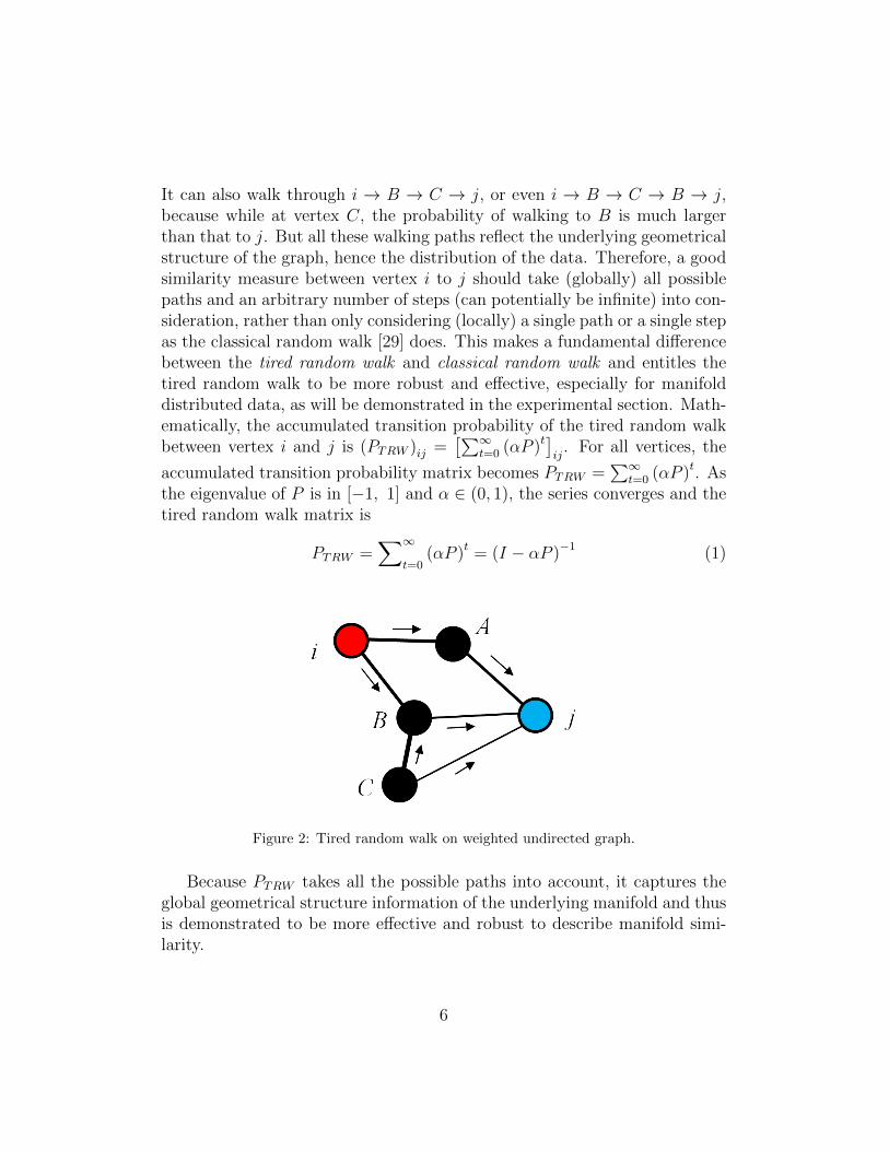
It can also walk through i → B → C → j, or even i → B → C → B → j,because while at vertex C, the probability of walking to B is much largerthan that to j. But all these walking paths reflect the underlying geometricalstructure of the graph, hence the distribution of the data. Therefore, a goodsimilarity measure between vertex i to j should take (globally) all possiblepaths and an arbitrary number of steps (can potentially be infinite) into con-sideration, rather than only considering (locally) a single path or a single stepas the classical random walk [29] does. This makes a fundamental differencebetween the tired random walk and classical random walk and entitles thetired random walk to be more robust and effective, especially for manifolddistributed data, as will be demonstrated in the experimental section. Math-ematically, the accumulated transition probability of the tired random walkbetween vertex i and j is (PTRW )ij =

[∑∞t=0 (αP )t

]ij

. For all vertices, the

accumulated transition probability matrix becomes PTRW =∑∞

t=0 (αP )t. Asthe eigenvalue of P is in [−1, 1] and α ∈ (0, 1), the series converges and thetired random walk matrix is

PTRW =∑∞

t=0(αP )t = (I − αP )−1 (1)

Figure 2: Tired random walk on weighted undirected graph.

Because PTRW takes all the possible paths into account, it captures theglobal geometrical structure information of the underlying manifold and thusis demonstrated to be more effective and robust to describe manifold simi-larity.

6

3. A constrained tired random walk model

In this section, we further extend the model into a constrained situation.For classification purposes, we find that labeled samples provide not onlyclass distribution information, but also constraint information, i.e., sampleswhich have the same class labels are must-link pairs and samples which havedifferent class labels are cannot-link pairs. In most of the existing supervisedlearning algorithms, only class information is utilized but constraint infor-mation is discarded. Here we include constraint information into the TRWmodel by modifying the weights of graph edges between the labeled samples,because constraint information has been demonstrated to be useful for per-formance improvement [11, 15, 45, 58]. Class information will be utilized inthe next section for the proposed new kNN algorithm.

We first construct an R-level nearest-neighbor strengthened tree for eachlabeled sample xi ∈ XT as follows:

(i). Set xi as the first level node (tree root node, r = 0) and its k nearestneighbors as the second level nodes.

(ii). For each node in level r − 1, set its nearest neighbors as its level rdescendants. If any node in level r appears in its ancestor level, removeit from level r.

(iii). If r < R, go to (ii).

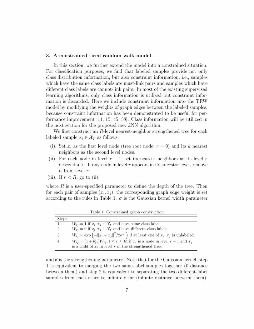
where R is a user-specified parameter to define the depth of the tree. Thenfor each pair of samples (xi, xj), the corresponding graph edge weight is setaccording to the rules in Table 1. σ is the Gaussian kernel width parameter

Table 1: Constrained graph construction

Steps1 Wij = 1 if xi, xj ∈ XT and have same class label.2 Wij = 0 if xi, xj ∈ XT and have different class labels.

3 Wij = exp(−‖xi − xj‖2/2σ2

)if at least one of xi, xj is unlabeled.

4 Wij = (1 + θrij)Wij , 1 ≤ r ≤ R, if xi is a node in level r − 1 and xjis a child of xi in level r in the strengthened tree.

and θ is the strengthening parameter. Note that for the Gaussian kernel, step1 is equivalent to merging the two same-label samples together (0 distancebetween them) and step 2 is equivalent to separating the two different-labelsamples from each other to infinitely far (infinite distance between them).

7

The connections from a labeled sample to its nearest neighbors are strength-ened by θij in step 4. This can spread the hard constraints in steps 1 and2 to farther neighborhoods on the graph in a form of soft constraints andthus causes these constraints to have a wider influence. The motivation ofconstructing the strengthened tree is inspired by the neural network reser-voir structure analysis techniques, in which information has been shown tospread out from input neurons to interior neurons in the reservoir followinga tree-structure path [43].

The selection of parameter θ is based the following conditions

• the strengthened weight should be positive and less than the weight ofthe must-link constraint.

• the strengthening effect should be positive and decays along the strength-ened tree level.

Mathematically, the conditions are{0 < Wij + θijWij < 1

0 < θr+1ij < θrij

(2)

As a result, θ should be

0 < θij < min

(1−Wij

Wij

, 1

)= θ̄ (3)

In all our experiments, we used a single value of θ = 0.1θ̄, which gives goodresults for both synthetic and real-world data.

4. A new graph-based kNN classification algorithm on nonlinearmanifold

Here we present a graph-based kNN algorithm for nonlinear manifolddata classification. The procedure of the algorithm is summarized in Table2.

Specifically, given PTRW matrix, the TRW weight between sample xi andxj is defined as

w̄ij = w(xi, xj) =(PTRW )ij + (PTRW )ji

2(4)

8

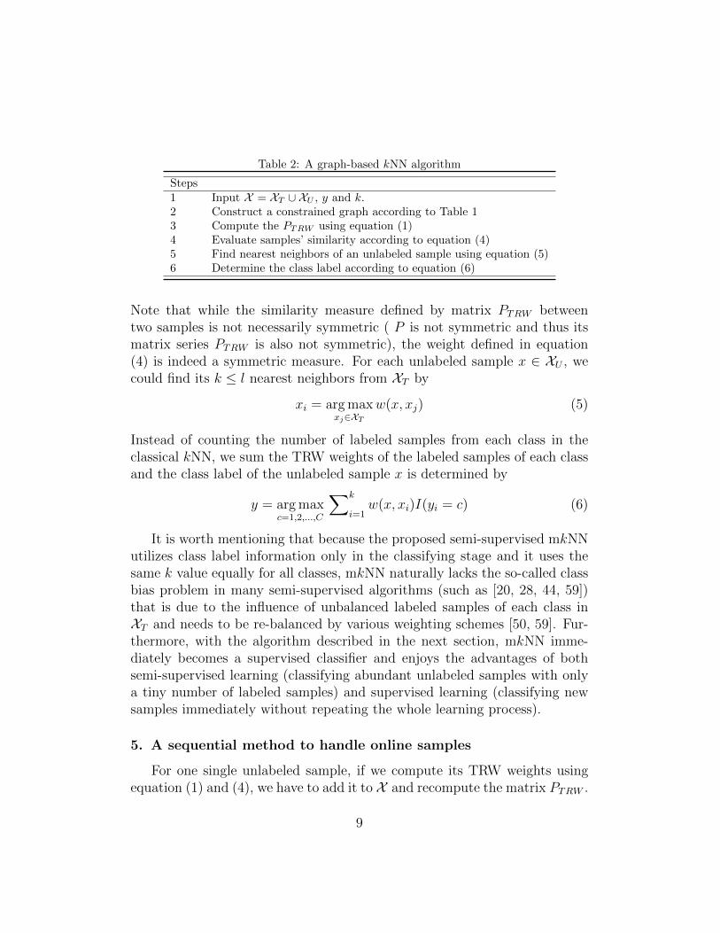
Table 2: A graph-based kNN algorithm

Steps1 Input X = XT ∪ XU , y and k.2 Construct a constrained graph according to Table 13 Compute the PTRW using equation (1)4 Evaluate samples’ similarity according to equation (4)5 Find nearest neighbors of an unlabeled sample using equation (5)6 Determine the class label according to equation (6)

Note that while the similarity measure defined by matrix PTRW betweentwo samples is not necessarily symmetric ( P is not symmetric and thus itsmatrix series PTRW is also not symmetric), the weight defined in equation(4) is indeed a symmetric measure. For each unlabeled sample x ∈ XU , wecould find its k ≤ l nearest neighbors from XT by

xi = arg maxxj∈XT

w(x, xj) (5)

Instead of counting the number of labeled samples from each class in theclassical kNN, we sum the TRW weights of the labeled samples of each classand the class label of the unlabeled sample x is determined by

y = arg maxc=1,2,...,C

∑k

i=1w(x, xi)I(yi = c) (6)

It is worth mentioning that because the proposed semi-supervised mkNNutilizes class label information only in the classifying stage and it uses thesame k value equally for all classes, mkNN naturally lacks the so-called classbias problem in many semi-supervised algorithms (such as [20, 28, 44, 59])that is due to the influence of unbalanced labeled samples of each class inXT and needs to be re-balanced by various weighting schemes [50, 59]. Fur-thermore, with the algorithm described in the next section, mkNN imme-diately becomes a supervised classifier and enjoys the advantages of bothsemi-supervised learning (classifying abundant unlabeled samples with onlya tiny number of labeled samples) and supervised learning (classifying newsamples immediately without repeating the whole learning process).

5. A sequential method to handle online samples

For one single unlabeled sample, if we compute its TRW weights usingequation (1) and (4), we have to add it to X and recompute the matrix PTRW .

9

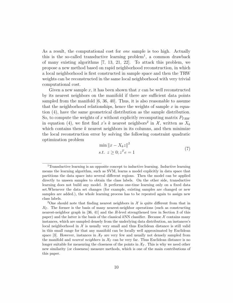
As a result, the computational cost for one sample is too high. Actuallythis is the so-called transductive learning problem1, a common drawbackof many existing algorithms [7, 13, 21, 22]. To attack this problem, wepropose a new method based on rapid neighborhood reconstruction, in whicha local neighborhood is first constructed in sample space and then the TRWweights can be reconstructed in the same local neighborhood with very trivialcomputational cost.

Given a new sample x, it has been shown that x can be well reconstructedby its nearest neighbors on the manifold if there are sufficient data pointssampled from the manifold [6, 36, 40]. Thus, it is also reasonable to assumethat the neighborhood relationships, hence the weights of sample x in equa-tion (4), have the same geometrical distribution as the sample distribution.So, to compute the weights of x without explicitly recomputing matrix PTRW

in equation (4), we first find x’s k nearest neighbors2 in X , written as Xk

which contains these k nearest neighbors in its columns, and then minimizethe local reconstruction error by solving the following constraint quadraticoptimization problem

min ‖x−Xkz‖2

s.t. z ≥ 0; zT e = 1(7)

1Transductive learning is an opposite concept to inductive learning. Inductive learningmeans the learning algorithm, such as SVM, learns a model explicitly in data space thatpartitions the data space into several different regions. Then the model can be applieddirectly to unseen samples to obtain the class labels. On the other side, transductivelearning does not build any model. It performs one-time learning only on a fixed dataset.Whenever the data set changes (for example, existing samples are changed or newsamples are added.), the whole learning process has to be repeated again to assign newclass labels.

2One should note that finding nearest neighbors in X is quite different from that inXT . The former is the basis of many nearest-neighbor operations (such as constructingnearest-neighbor graph in [36, 41] and the R-level strengthened tree in Section 3 of thispaper) and the latter is the basis of the classical kNN classifier. Because X contains manyinstances, which are sampled densely from the underlying data distribution, an instances’slocal neighborhood in X is usually very small and thus Euclidean distance is still validin this small range for that any manifold can be locally well approximated by Euclideanspace [3]. However, instances in XT are very few and usually not densely sampled fromthe manifold and nearest neighbors in XT can be very far. Thus Euclidean distance is nolonger suitable for measuring the closeness of the points in XT . This is why we need othernew similarity (or closeness) measure methods, which is one of the main contributions ofthis paper.

10

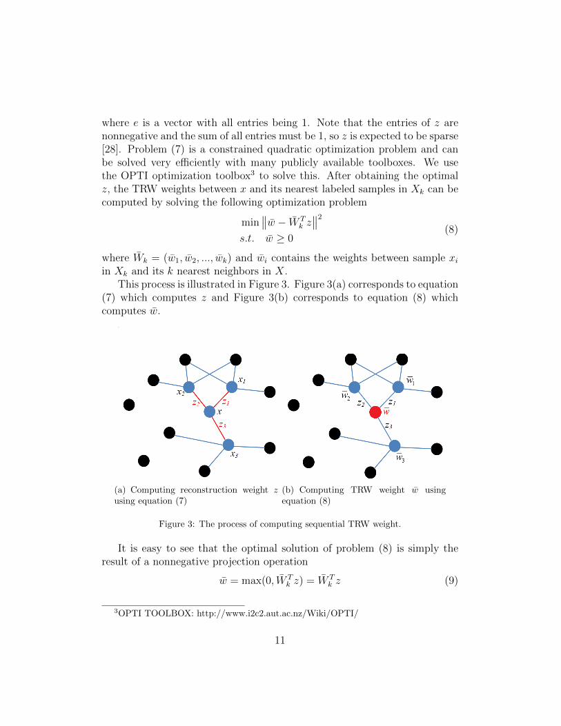
where e is a vector with all entries being 1. Note that the entries of z arenonnegative and the sum of all entries must be 1, so z is expected to be sparse[28]. Problem (7) is a constrained quadratic optimization problem and canbe solved very efficiently with many publicly available toolboxes. We usethe OPTI optimization toolbox3 to solve this. After obtaining the optimalz, the TRW weights between x and its nearest labeled samples in Xk can becomputed by solving the following optimization problem

min∥∥w̄ − W̄ T

k z∥∥2

s.t. w̄ ≥ 0(8)

where W̄k = (w̄1, w̄2, ..., w̄k) and w̄i contains the weights between sample xiin Xk and its k nearest neighbors in X.

This process is illustrated in Figure 3. Figure 3(a) corresponds to equation(7) which computes z and Figure 3(b) corresponds to equation (8) whichcomputes w̄.

(a) Computing reconstruction weight zusing equation (7)

(b) Computing TRW weight w̄ usingequation (8)

Figure 3: The process of computing sequential TRW weight.

It is easy to see that the optimal solution of problem (8) is simply theresult of a nonnegative projection operation

w̄ = max(0, W̄ Tk z) = W̄ T

k z (9)

3OPTI TOOLBOX: http://www.i2c2.aut.ac.nz/Wiki/OPTI/

11

The second equation holds because both W̄k and z are nonnegative andtherefore their multiplication result is also nonnegative.

One should note that with this sequential learning strategy, the proposedmkNN can be treated as an inductive classifier, whose model consists ofboth the PTRW matrix and the data samples that have been classified so far.Whenever a new sample arrives, the model can quickly give its class label bythe three steps in Table 3, without repeating the whole learning process inTable 2.

Table 3: The procedure of sequential manifold kNN algorithm

Steps1 Input X = XT ∪ XU , PTRW , x and k.2 Find x’s k nearest neighbors in X3 Use equations (7) and (8) to compute its TRW weights4 Use equation (6) to classify it

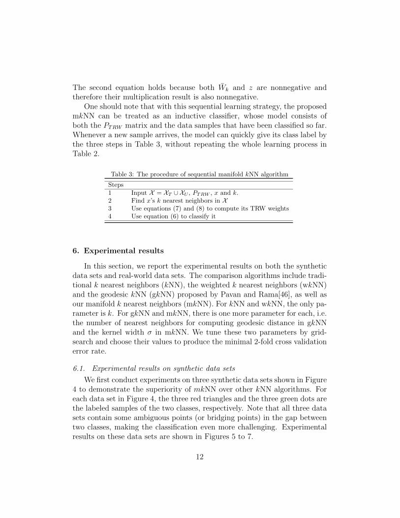
6. Experimental results

In this section, we report the experimental results on both the syntheticdata sets and real-world data sets. The comparison algorithms include tradi-tional k nearest neighbors (kNN), the weighted k nearest neighbors (wkNN)and the geodesic kNN (gkNN) proposed by Pavan and Rama[46], as well asour manifold k nearest neighbors (mkNN). For kNN and wkNN, the only pa-rameter is k. For gkNN and mkNN, there is one more parameter for each, i.e.the number of nearest neighbors for computing geodesic distance in gkNNand the kernel width σ in mkNN. We tune these two parameters by grid-search and choose their values to produce the minimal 2-fold cross validationerror rate.

6.1. Experimental results on synthetic data sets

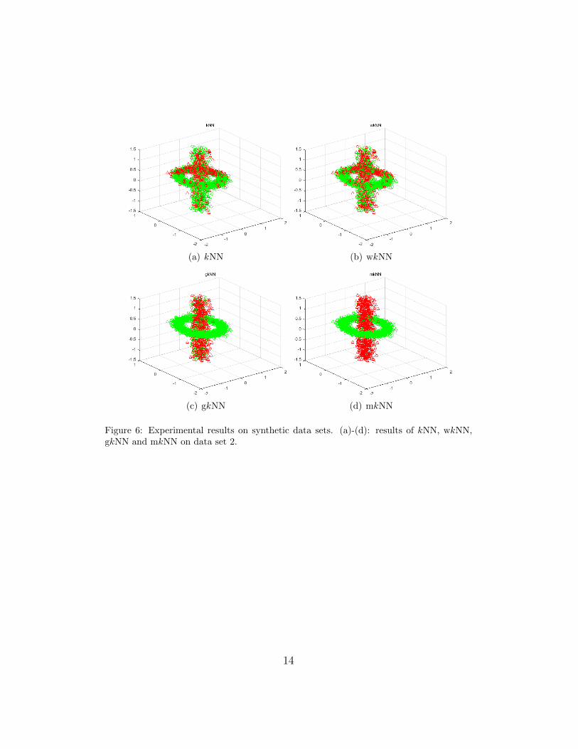
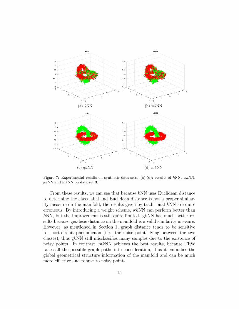
We first conduct experiments on three synthetic data sets shown in Figure4 to demonstrate the superiority of mkNN over other kNN algorithms. Foreach data set in Figure 4, the three red triangles and the three green dots arethe labeled samples of the two classes, respectively. Note that all three datasets contain some ambiguous points (or bridging points) in the gap betweentwo classes, making the classification even more challenging. Experimentalresults on these data sets are shown in Figures 5 to 7.

12

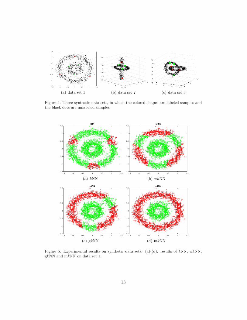
(a) data set 1 (b) data set 2 (c) data set 3

Figure 4: Three synthetic data sets, in which the colored shapes are labeled samples andthe black dots are unlabeled samples

(a) kNN (b) wkNN

(c) gkNN (d) mkNN

Figure 5: Experimental results on synthetic data sets. (a)-(d): results of kNN, wkNN,gkNN and mkNN on data set 1.

13

(a) kNN (b) wkNN

(c) gkNN (d) mkNN

Figure 6: Experimental results on synthetic data sets. (a)-(d): results of kNN, wkNN,gkNN and mkNN on data set 2.

14

(a) kNN (b) wkNN

(c) gkNN (d) mkNN

Figure 7: Experimental results on synthetic data sets. (a)-(d): results of kNN, wkNN,gkNN and mkNN on data set 3.

From these results, we can see that because kNN uses Euclidean distanceto determine the class label and Euclidean distance is not a proper similar-ity measure on the manifold, the results given by traditional kNN are quiteerroneous. By introducing a weight scheme, wkNN can perform better thankNN, but the improvement is still quite limited. gkNN has much better re-sults because geodesic distance on the manifold is a valid similarity measure.However, as mentioned in Section 1, graph distance tends to be sensitiveto short-circuit phenomenon (i.e. the noise points lying between the twoclasses), thus gkNN still misclassifies many samples due to the existence ofnoisy points. In contrast, mkNN achieves the best results, because TRWtakes all the possible graph paths into consideration, thus it embodies theglobal geometrical structure information of the manifold and can be muchmore effective and robust to noisy points.

15

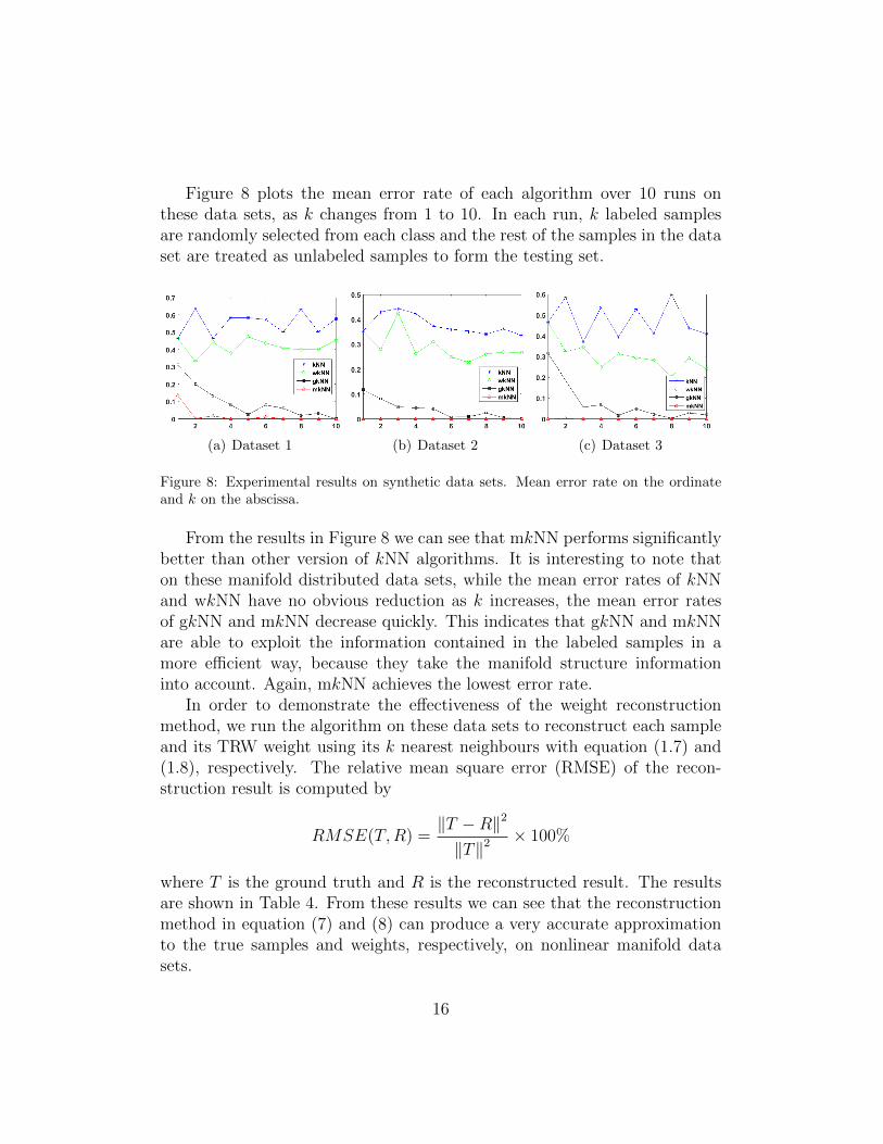
Figure 8 plots the mean error rate of each algorithm over 10 runs onthese data sets, as k changes from 1 to 10. In each run, k labeled samplesare randomly selected from each class and the rest of the samples in the dataset are treated as unlabeled samples to form the testing set.

(a) Dataset 1 (b) Dataset 2 (c) Dataset 3

Figure 8: Experimental results on synthetic data sets. Mean error rate on the ordinateand k on the abscissa.

From the results in Figure 8 we can see that mkNN performs significantlybetter than other version of kNN algorithms. It is interesting to note thaton these manifold distributed data sets, while the mean error rates of kNNand wkNN have no obvious reduction as k increases, the mean error ratesof gkNN and mkNN decrease quickly. This indicates that gkNN and mkNNare able to exploit the information contained in the labeled samples in amore efficient way, because they take the manifold structure informationinto account. Again, mkNN achieves the lowest error rate.

In order to demonstrate the effectiveness of the weight reconstructionmethod, we run the algorithm on these data sets to reconstruct each sampleand its TRW weight using its k nearest neighbours with equation (1.7) and(1.8), respectively. The relative mean square error (RMSE) of the recon-struction result is computed by

RMSE(T,R) =‖T −R‖2

‖T‖2× 100%

where T is the ground truth and R is the reconstructed result. The resultsare shown in Table 4. From these results we can see that the reconstructionmethod in equation (7) and (8) can produce a very accurate approximationto the true samples and weights, respectively, on nonlinear manifold datasets.

16

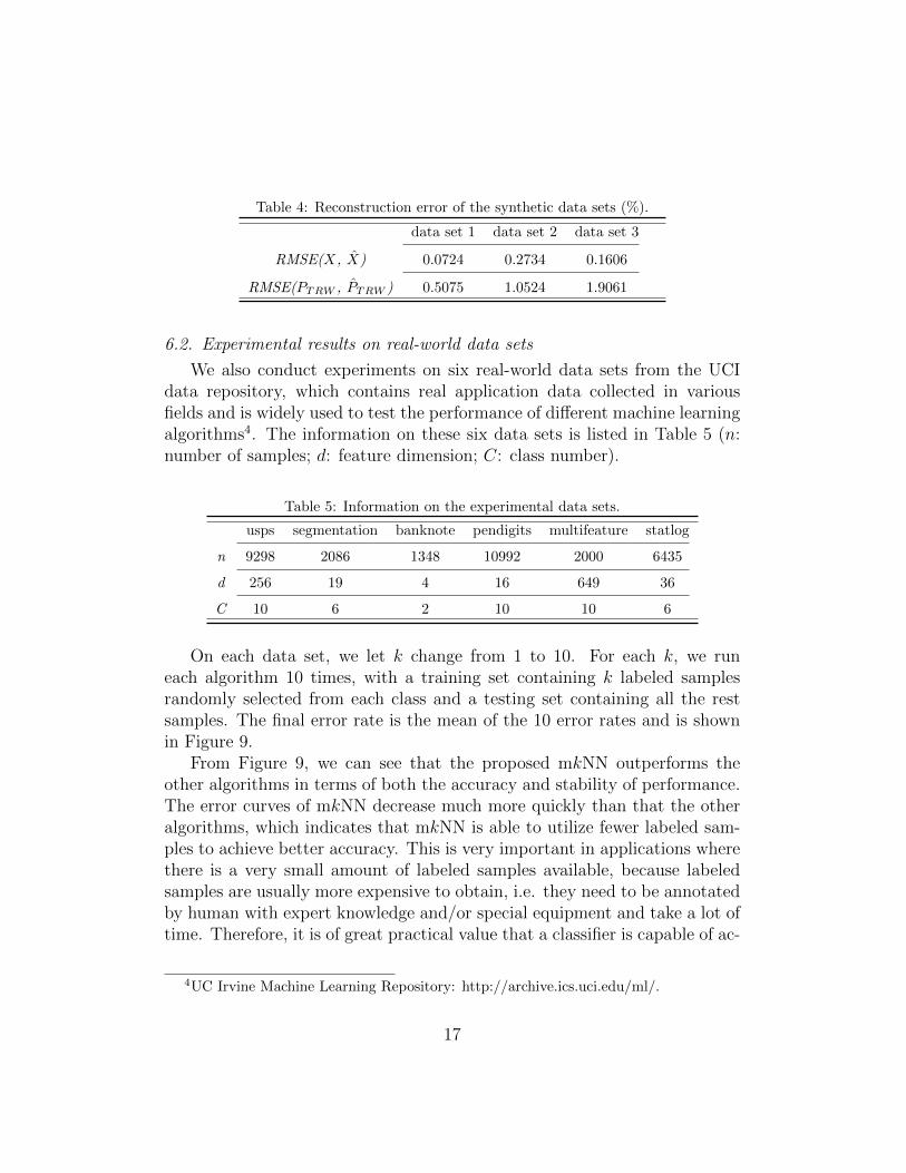
Table 4: Reconstruction error of the synthetic data sets (%).

data set 1 data set 2 data set 3

RMSE(X, X̂) 0.0724 0.2734 0.1606

RMSE(PTRW , P̂TRW ) 0.5075 1.0524 1.9061

6.2. Experimental results on real-world data sets

We also conduct experiments on six real-world data sets from the UCIdata repository, which contains real application data collected in variousfields and is widely used to test the performance of different machine learningalgorithms4. The information on these six data sets is listed in Table 5 (n:number of samples; d: feature dimension; C: class number).

Table 5: Information on the experimental data sets.

usps segmentation banknote pendigits multifeature statlog

n 9298 2086 1348 10992 2000 6435

d 256 19 4 16 649 36

C 10 6 2 10 10 6

On each data set, we let k change from 1 to 10. For each k, we runeach algorithm 10 times, with a training set containing k labeled samplesrandomly selected from each class and a testing set containing all the restsamples. The final error rate is the mean of the 10 error rates and is shownin Figure 9.

From Figure 9, we can see that the proposed mkNN outperforms theother algorithms in terms of both the accuracy and stability of performance.The error curves of mkNN decrease much more quickly than that the otheralgorithms, which indicates that mkNN is able to utilize fewer labeled sam-ples to achieve better accuracy. This is very important in applications wherethere is a very small amount of labeled samples available, because labeledsamples are usually more expensive to obtain, i.e. they need to be annotatedby human with expert knowledge and/or special equipment and take a lot oftime. Therefore, it is of great practical value that a classifier is capable of ac-

4UC Irvine Machine Learning Repository: http://archive.ics.uci.edu/ml/.

17

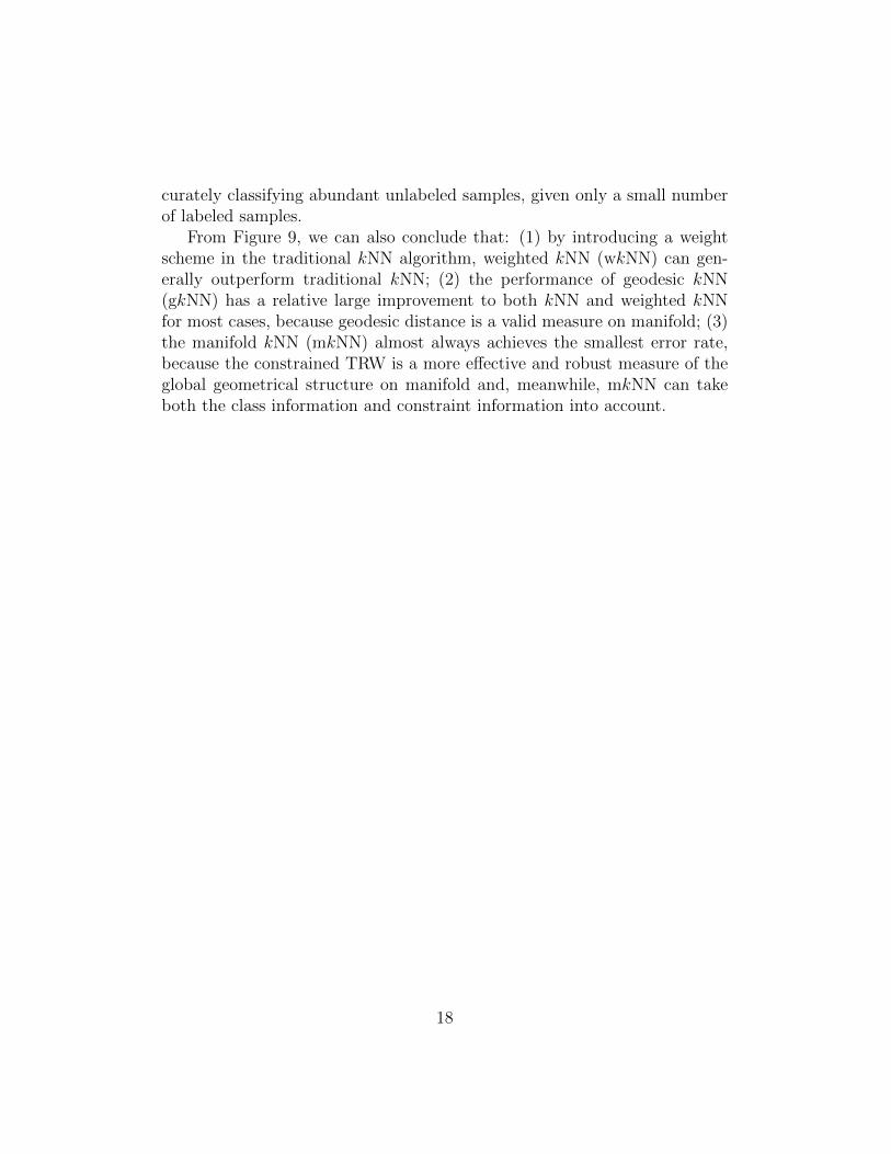
curately classifying abundant unlabeled samples, given only a small numberof labeled samples.

From Figure 9, we can also conclude that: (1) by introducing a weightscheme in the traditional kNN algorithm, weighted kNN (wkNN) can gen-erally outperform traditional kNN; (2) the performance of geodesic kNN(gkNN) has a relative large improvement to both kNN and weighted kNNfor most cases, because geodesic distance is a valid measure on manifold; (3)the manifold kNN (mkNN) almost always achieves the smallest error rate,because the constrained TRW is a more effective and robust measure of theglobal geometrical structure on manifold and, meanwhile, mkNN can takeboth the class information and constraint information into account.

18

(a) usps (b) segmentation

(c) banknote (d) pendigits

(e) multifeature (f) satlog

Figure 9: Experimental results on six real-world data sets. Mean error rate on the ordinateand k on the abscissa.

19

6.3. Experimental results of the comparison with other traditional supervisedclassifiers

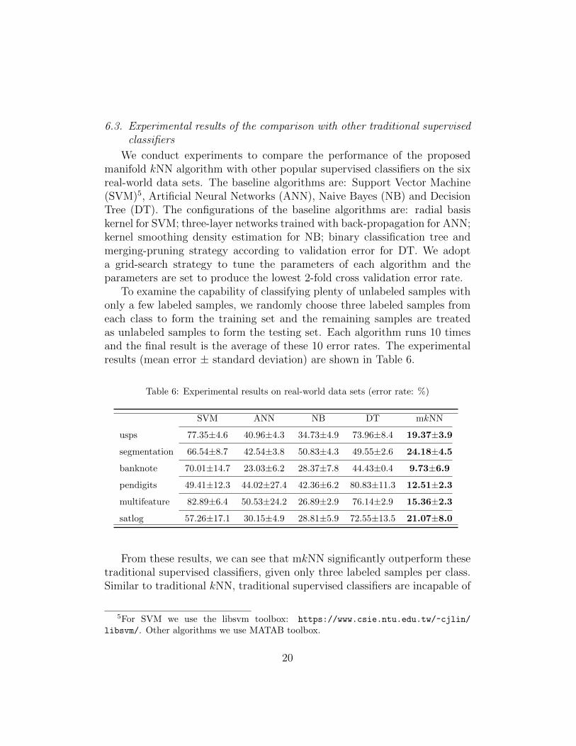
We conduct experiments to compare the performance of the proposedmanifold kNN algorithm with other popular supervised classifiers on the sixreal-world data sets. The baseline algorithms are: Support Vector Machine(SVM)5, Artificial Neural Networks (ANN), Naive Bayes (NB) and DecisionTree (DT). The configurations of the baseline algorithms are: radial basiskernel for SVM; three-layer networks trained with back-propagation for ANN;kernel smoothing density estimation for NB; binary classification tree andmerging-pruning strategy according to validation error for DT. We adopta grid-search strategy to tune the parameters of each algorithm and theparameters are set to produce the lowest 2-fold cross validation error rate.

To examine the capability of classifying plenty of unlabeled samples withonly a few labeled samples, we randomly choose three labeled samples fromeach class to form the training set and the remaining samples are treatedas unlabeled samples to form the testing set. Each algorithm runs 10 timesand the final result is the average of these 10 error rates. The experimentalresults (mean error ± standard deviation) are shown in Table 6.

Table 6: Experimental results on real-world data sets (error rate: %)

SVM ANN NB DT mkNN

usps 77.35±4.6 40.96±4.3 34.73±4.9 73.96±8.4 19.37±3.9

segmentation 66.54±8.7 42.54±3.8 50.83±4.3 49.55±2.6 24.18±4.5

banknote 70.01±14.7 23.03±6.2 28.37±7.8 44.43±0.4 9.73±6.9

pendigits 49.41±12.3 44.02±27.4 42.36±6.2 80.83±11.3 12.51±2.3

multifeature 82.89±6.4 50.53±24.2 26.89±2.9 76.14±2.9 15.36±2.3

satlog 57.26±17.1 30.15±4.9 28.81±5.9 72.55±13.5 21.07±8.0

From these results, we can see that mkNN significantly outperform thesetraditional supervised classifiers, given only three labeled samples per class.Similar to traditional kNN, traditional supervised classifiers are incapable of

5For SVM we use the libsvm toolbox: https://www.csie.ntu.edu.tw/~cjlin/

libsvm/. Other algorithms we use MATAB toolbox.

20

exploiting the manifold structure information of the underlying data distri-bution, thus their accuracies are very low while the labeled sample numberis very small. Furthermore, when the labeled samples are randomly selected,their positions vary greatly in data space. Sometime they are not uniformlydistributed and thus cannot well cover the whole data distribution. As aresult, the performance of traditional classifiers also varies greatly. In con-trast, because mkNN adopts tired random walk to measure manifold sim-ilarity which reflects the global geometrical information of the underlyingmanifold structure and is robust to local changes. [42], it can achieve muchbetter results.

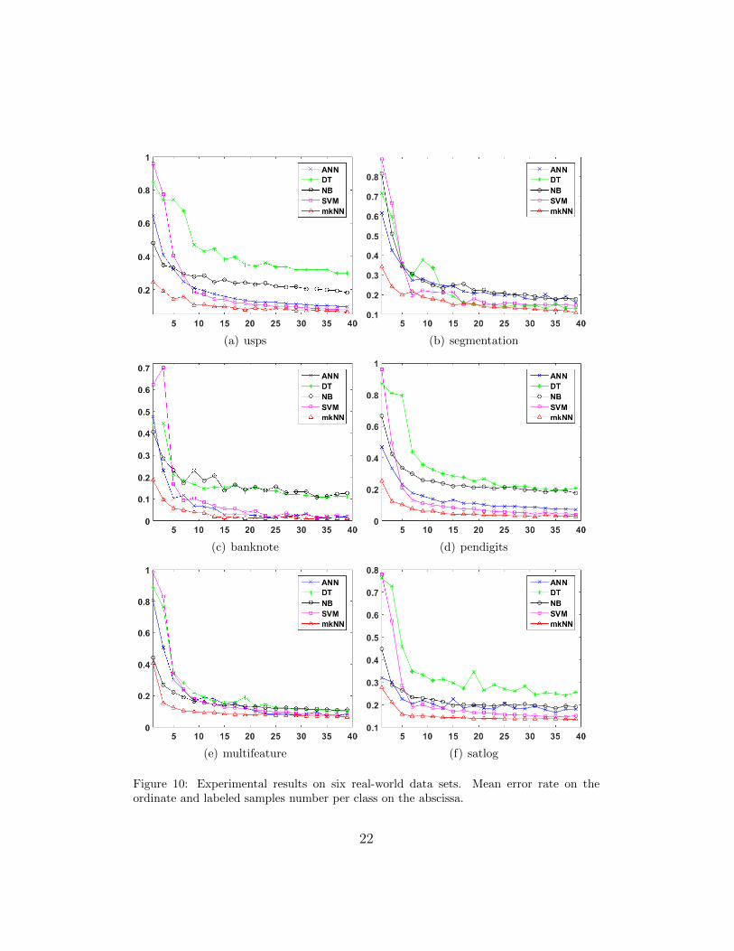
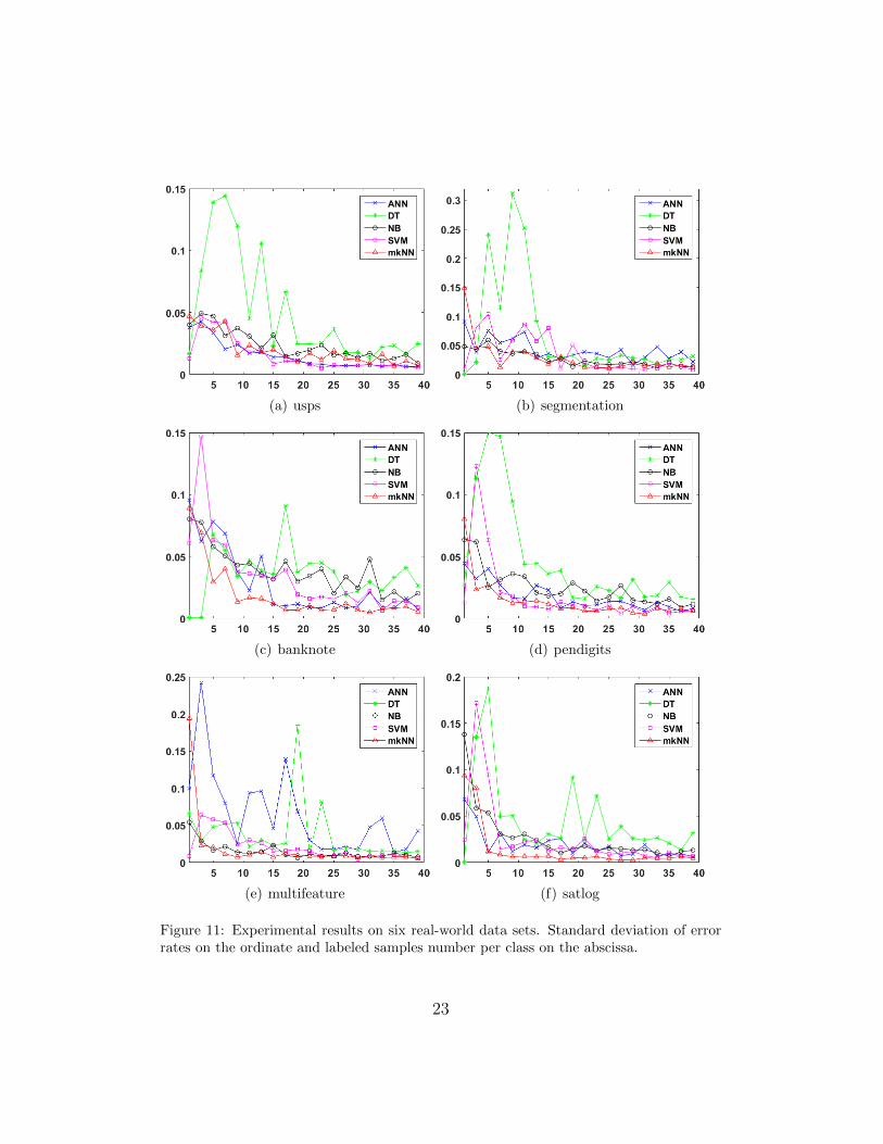
To further investigate the performance of these algorithms under the con-dition of providing different number of training samples, we carry out exper-iments with different training set sizes. For each data set, we let k variesfrom 1 to 40 (k = 1, 3, ..., 39) and randomly choose k labeled samples fromeach class to form the training set. The rest of the data set are treated asunlabeled samples to test each algorithm’s performance. For each k, everyalgorithm runs 10 times on each data set. The mean error rate and standarddeviation of the 10-run results are shown in Figures 10 and 11, respectively.

From Figure 10 we can see that while the labeled sample number is small,the error rates of the traditional algorithms are very large (as also indicatedin Table 6 which contains the results of the three labeled samples per class).As the number of labeled sample increases, the error rates decrease. Thistrend becomes slower after 15 labeled samples per class. The proposed mkNNachieves the lowest error rate for both situations of small and large numberof labeled samples. The improvement is especially obvious and significantwhen the labeled samples number is small. From Figure 11, we can also seethat the performance of mkNN is also relatively steady for most cases. Oneshould note that on the left of each plot in Figure 11, the small standarddeviation values of decision tree (DT) and SVM are due to the fact thattheir error rates are always very high in each run (e.g. the error rates ofSVM on data set usps concentrate closely around 95).

21

(a) usps (b) segmentation

(c) banknote (d) pendigits

(e) multifeature (f) satlog

Figure 10: Experimental results on six real-world data sets. Mean error rate on theordinate and labeled samples number per class on the abscissa.

22

(a) usps (b) segmentation

(c) banknote (d) pendigits

(e) multifeature (f) satlog

Figure 11: Experimental results on six real-world data sets. Standard deviation of errorrates on the ordinate and labeled samples number per class on the abscissa.

23

6.4. Experimental results of time complexity

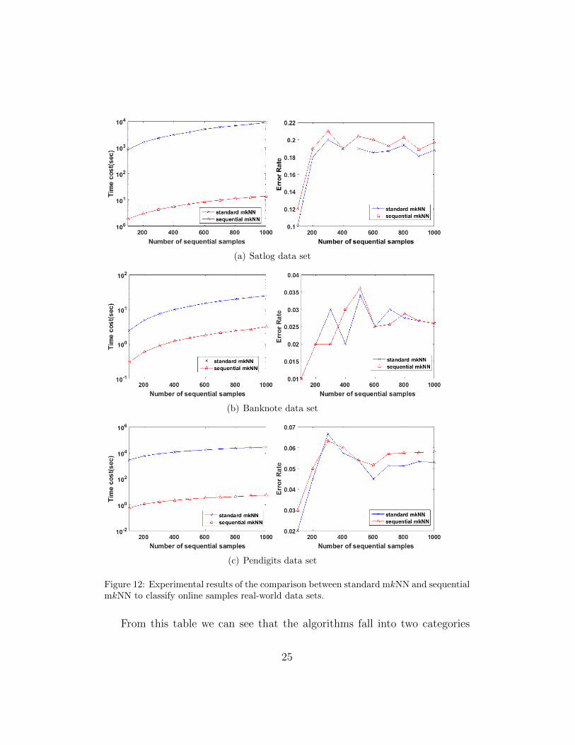
To examine the effectiveness and efficiency of the proposed sequentiallearning strategy in Section 5, we conduct experiments on three real-worlddata sets banknote,satlog and pendigits to show the difference of mkNN’sperformance with and without sequential learning algorithm. Each data setis divided into three subsets: training set, validation set and online set. Thetraining set is fixed to contain 10 labeled samples per class. We conduct 10experiments, with the online set size changes from 100 to 1000 with step size100. The validation set contains the rest of the samples. First, mkNN runson training set and validation set to learn the class distribution. Thereafter,at each time a sample is drawn from the online set as a new coming sample.For sequential mkNN, the previous learning result is used to classify the newsample according to equation (7) and equation (8). For standard mkNN, thenew sample is added to the validation set and the whole learning process isrepeated to classify the new sample. The experimental results6 are shown inFigure 12.

From these results, we can see that while the classification accuracy ofstandard mkNN and sequential mkNN are comparable, the time cost of se-quential mkNN reduces dramatically for online classification (e.g., for satlogdata set, to classify 1000 sequentially coming samples, standard mkNN takesabout 9100 seconds but sequential mkNN uses only about 14 seconds toachieve a similar result). Therefore, the sequential algorithm has great meritin solving the online classification problem and can be potentially applied toa wide range of transductive learning algorithms to make them inductive.

We also conduct experiments to compare the time complexity of all thebaseline algorithms with the proposed mkNN on these three data sets. Eachdata set is split into training and testing parts three times independently,with splitting ratios 10%, 25% and 50%, respectively. For each split, everyalgorithm runs 10 times and the mean time cost is recorded. Table 7 showsthe experimental results (the second column shows the splitting ratio).

6The configuration of our computer: 16GB RAM, double-core 3.7GHz Intel Xeon CPUand MATLAB 2015 academic version.

24

(a) Satlog data set

(b) Banknote data set

(c) Pendigits data set

Figure 12: Experimental results of the comparison between standard mkNN and sequentialmkNN to classify online samples real-world data sets.

From this table we can see that the algorithms fall into two categories

25

Table 7: Comparison of overall time for training and testing on three data sets (sec)

data (%) SVM DT ANN NB kNN wkNN gkNN mkNN

10 0.01 0.14 0.23 0.09 0.03 0.02 1.23 0.19

banknote 25 0.01 0.19 0.24 0.09 0.04 0.03 1.23 0.20

50 0.02 0.29 0.27 0.08 0.05 0.05 1.26 0.20

10 0.47 0.43 0.59 7.14 0.13 0.14 31.99 6.01

satlog 25 1.78 1.16 1.58 7.56 0.24 0.29 32.55 6.08

50 5.12 3.11 4.01 7.61 0.31 0.40 32.82 6.30

10 0.44 0.78 0.70 8.70 0.22 0.28 149.14 25.27

pendigits 25 0.86 2.28 2.65 8.46 0.41 0.59 146.89 26.11

50 1.55 6.09 5.06 6.93 0.54 0.80 145.71 25.35

according to their time costs: one category contains SVM, DT, ANN, kNNand wkNN, whose time costs are closely related with the training data setsize. Another category includes NB, gkNN and mkNN, whose time costs de-pend more upon the overall data set size. SVM, kNN and wkNN are generallyfaster than others. Although mkNN is the second slowest one, it is still muchfaster than gkNN and its overall time does not prolong as the training set sizeincreases. It should be mentioned that although the classification accuracy ofmkNN is much better than kNN and other traditional supervised classifiers,the computational complexity of mkNN is also higher (O(n3)) than tradi-tional kNN (O(n)). Directly computing PTRW matrix is time cost, since it isnot symmetrical, positive definite matrix and thus a LU decomposition has tobe used. One way to speed-up matrix inverse is to convert PTRW to a symmet-rical, positive definite matrix and then adopt the Cholesky decomposition,whose computational cost is just a half of the LU decomposition [14]. Not-

ing that PTRW = (I − αD−1W )−1

= D1/2(I − αD−1/2WD−1/2

)−1D−1/2 =

D1/2R−1D−1/2, where R = I − αD−1/2WD−1/2 is a symmetrical, positivedefinite matrix7, we can first inverse matrix R using Cholesky decompositionand then compute PTRW with very small computational cost. Our followingwork will be focused on the further reduction of computational complexity.

7R is apparently symmetrical because W is symmetrical (Let W = (W +WT )/2 if Wis not symmetrical). We prove its positive definiteness. Because the spectral radius ofPTRW is in (0, 1) and PTRW is similar to R−1, so spectral radius of R−1 is in (0, 1). Soall eigenvalues of R are positive. Therefore R is a positive definite, symmetrical matrix.

26

7. Conclusions

In this paper we proposed a new k nearest-neighbor algorithm, mkNN, toclassify nonlinear manifold distributed data as well as traditional Gaussiandistributed data, given a very small amount of labeled samples. We alsopresented an algorithm to attack the problem of high computational cost forclassifying online data with mkNN and other transductive algorithms. Thesuperiority of the mkNN has been demonstrated by substantial experimentson both synthetic data sets and real-world data sets. Given the widespreadappearance of manifold structures in real-world problems and the popularityof the traditional kNN algorithm, the proposed manifold version kNN showspromising potential for classifying manifold-distributed data.

Acknowledgements: The authors wish to thank the anonymous review-ers for reading the entire manuscript and offering many useful suggestions.This research is partly supported by NSFC, China (No: 61572315) and 973PlanChina (No. 2015CB856004). The research is also partly supported byYangFan Project (Grant No. 14YF1411000) of Shanghai Municipal Scienceand Technology Commission, the Innovation Program (Grant No. 14YZ131)and the Excellent Youth Scholars (Grant No. sdl15101) of Shanghai Munic-ipal Education Commission, the Science Research Foundation of ShanghaiUniversity of Electric Power (Grant No. K2014-032).

References

[1] Bengio, Y., Larochelle, H., Vincent, P., 2005. Non-local manifold parzenwindows. In: Advances in neural information processing systems. pp.115–122.

[2] Beyer, K., Goldstein, J., Ramakrishnan, R., Shaft, U., 1999. When isnearest neighbor meaningful? In: Database TheoryICDT99. Springer,pp. 217–235.

[3] Boothby, W. M., 2003. An introduction to differentiable manifolds andRiemannian geometry. Vol. 120. Gulf Professional Publishing.

[4] Camastra, F., Staiano, A., 2016. Intrinsic dimension estimation: Ad-vances and open problems. Information Sciences 328, 26–41.

27

[5] Chahooki, M. A. Z., Charkari, N. M., 2014. Shape classification by man-ifold learning in multiple observation spaces. Information Sciences 262,46–61.

[6] Chen, Y., Zhang, J., Cai, D., Liu, W., He, X., 2013. Nonnegative lo-cal coordinate factorization for image representation. Image Processing,IEEE Transactions on 22 (3), 969–979.

[7] Collobert, R., Sinz, F., Weston, J., Bottou, L., 2006. Large scale trans-ductive svms. The Journal of Machine Learning Research 7, 1687–1712.

[8] Cost, S., Salzberg, S., 1993. A weighted nearest neighbor algorithm forlearning with symbolic features. Machine learning 10 (1), 57–78.

[9] Cover, T. M., Hart, P. E., 1967. Nearest neighbor pattern classification.Information Theory, IEEE Transactions on 13 (1), 21–27.

[10] Dudani, S. A., 1976. The distance-weighted k-nearest-neighbor rule. Sys-tems, Man and Cybernetics, IEEE Transactions on (4), 325–327.

[11] Fu, Z., Lu, Z., Ip, H. H., Lu, H., Wang, Y., 2015. Local similaritylearning for pairwise constraint propagation. Multimedia Tools and Ap-plications 74 (11), 3739–3758.

[12] Gao, Y., Liu, Q., Miao, X., Yang, J., 2016. Reverse k-nearest neighborsearch in the presence of obstacles. Information Sciences 330, 274–292.

[13] Goldberg, A., Recht, B., Xu, J., Nowak, R., Zhu, X., 2010. Transductionwith matrix completion: Three birds with one stone. In: Advances inneural information processing systems. pp. 757–765.

[14] Golub, G. H., Van Loan, C. F., 2012. Matrix computations. Vol. 3. JHUPress.

[15] Gong, C., Fu, K., Wu, Q., Tu, E., Yang, J., 2014. Semi-supervisedclassification with pairwise constraints. Neurocomputing 139, 130–137.

[16] Han, E.-H. S., Karypis, G., Kumar, V., 2001. Text categorization usingweight adjusted k-nearest neighbor classification. Springer.

28

[17] Hastie, T., Tibshirani, R., 1996. Discriminant adaptive nearest neighborclassification. Pattern Analysis and Machine Intelligence, IEEE Trans-actions on 18 (6), 607–616.

[18] He, Q. P., Wang, J., 2007. Fault detection using the k-nearest neighborrule for semiconductor manufacturing processes. Semiconductor manu-facturing, IEEE transactions on 20 (4), 345–354.

[19] Hechenbichler, K., Schliep, K., 2004. Weighted k-nearest-neighbor tech-niques and ordinal classification.

[20] Ji, P., Zhao, N., Hao, S., Jiang, J., 2014. Automatic image annotationby semi-supervised manifold kernel density estimation. Information Sci-ences 281, 648–660.

[21] Joachims, T., 1999. Transductive inference for text classification usingsupport vector machines. In: ICML. Vol. 99. pp. 200–209.

[22] Joachims, T., et al., 2003. Transductive learning via spectral graph par-titioning. In: ICML. Vol. 3. pp. 290–297.

[23] Kolahdouzan, M., Shahabi, C., 2004. Voronoi-based k nearest neighborsearch for spatial network databases. In: Proceedings of the Thirtiethinternational conference on Very large data bases-Volume 30. VLDBEndowment, pp. 840–851.

[24] Kowalski, B., Bender, C., 1972. k-nearest neighbor classification rule(pattern recognition) applied to nuclear magnetic resonance spectral in-terpretation. Analytical Chemistry 44 (8), 1405–1411.

[25] Li, B., Yu, S., Lu, Q., 2003. An improved k-nearest neighbor algorithmfor text categorization. arXiv preprint cs/0306099.

[26] Li, L., Darden, T. A., Weingberg, C., Levine, A., Pedersen, L. G., 2001.Gene assessment and sample classification for gene expression data usinga genetic algorithm/k-nearest neighbor method. Combinatorial chem-istry & high throughput screening 4 (8), 727–739.

[27] Liao, Y., Vemuri, V. R., 2002. Use of k-nearest neighbor classifier forintrusion detection. Computers & Security 21 (5), 439–448.

29

[28] Liu, W., He, J., Chang, S.-F., 2010. Large graph construction for scal-able semi-supervised learning. In: Proceedings of the 27th internationalconference on machine learning (ICML-10). pp. 679–686.

[29] Luxburg, U. V., Radl, A., Hein, M., 2010. Getting lost in space: Largesample analysis of the resistance distance. In: Advances in Neural In-formation Processing Systems. pp. 2622–2630.

[30] Ma, L., Crawford, M. M., Tian, J., 2010. Local manifold learning-based-nearest-neighbor for hyperspectral image classification. Geoscience andRemote Sensing, IEEE Transactions on 48 (11), 4099–4109.

[31] Maltamo, M., Kangas, A., 1998. Methods based on k-nearest neighborregression in the prediction of basal area diameter distribution. Cana-dian Journal of Forest Research 28 (8), 1107–1115.

[32] Nene, S., Nayar, S. K., et al., 1997. A simple algorithm for nearestneighbor search in high dimensions. Pattern Analysis and Machine In-telligence, IEEE Transactions on 19 (9), 989–1003.

[33] Nowakowska, E., Koronacki, J., Lipovetsky, S., 2016. Dimensionalityreduction for data of unknown cluster structure. Information Sciences330, 74–87.

[34] Percus, A. G., Martin, O. C., 1998. Scaling universalities ofkth-nearestneighbor distances on closed manifolds. advances in applied mathematics21 (3), 424–436.

[35] Petraglia, A., et al., 2015. Dimensional reduction in constrained globaloptimization on smooth manifolds. Information Sciences 299, 243–261.

[36] Roweis, S. T., Saul, L. K., 2000. Nonlinear dimensionality reduction bylocally linear embedding. Science 290 (5500), 2323–2326.

[37] Samanthula, B. K., Elmehdwi, Y., Jiang, W., 2015. K-nearest neighborclassification over semantically secure encrypted relational data. Knowl-edge and Data Engineering, IEEE Transactions on 27 (5), 1261–1273.

[38] Spivak, M., 1970. A comprehensive introduction to differential geometry,vol. 2. I (Boston, Mass., 1970).

30

[39] Tan, S., 2005. Neighbor-weighted k-nearest neighbor for unbalanced textcorpus. Expert Systems with Applications 28 (4), 667–671.

[40] Tao, D., Cheng, J., Lin, X., Yu, J., 2015. Local structure preservingdiscriminative projections for rgb-d sensor-based scene classification. In-formation Sciences 320, 383–394.

[41] Tenenbaum, J. B., De Silva, V., Langford, J. C., 2000. A globalgeometric framework for nonlinear dimensionality reduction. Science290 (5500), 2319–2323.

[42] Tu, E., Cao, L., Yang, J., Kasabov, N., 2014. A novel graph-basedk-means for nonlinear manifold clustering and representative selection.Neurocomputing 143, 109–122.

[43] Tu, E., Kasabov, N., Yang, J., 2016. Mapping temporal variables intothe neucube for improved pattern recognition, predictive modeling, andunderstanding of stream data.

[44] Tu, E., Yang, J., Fang, J., Jia, Z., Kasabov, N., 2013. An experimen-tal comparison of semi-supervised learning algorithms for multispectralimage classification. Photogrammetric Engineering & Remote Sensing79 (4), 347–357.

[45] Tu, E., Yang, J., Kasabov, N., Zhang, Y., 2015. Posterior distribu-tion learning (pdl): A novel supervised learning framework using un-labeled samples to improve classification performance. Neurocomputing157, 173–186.

[46] Turaga, P., Chellappa, R., 2010. Nearest-neighbor search algorithms onnon-euclidean manifolds for computer vision applications. In: Proceed-ings of the Seventh Indian Conference on Computer Vision, Graphicsand Image Processing. ACM, pp. 282–289.

[47] Vemulapalli, R., Pillai, J. K., Chellappa, R., 2013. Kernel learning forextrinsic classification of manifold features. In: Computer Vision andPattern Recognition (CVPR), 2013 IEEE Conference on. IEEE, pp.1782–1789.

[48] Vincent, P., Bengio, Y., 2002. Manifold parzen windows. In: Advancesin neural information processing systems. pp. 825–832.

31

[49] Wang, H., Wu, J., Yuan, S., Chen, J., 2015. On characterizing scaleeffect of chinese mutual funds via text mining. Signal Processing.

[50] Wang, J., Jebara, T., Chang, S.-F., 2013. Semi-supervised learning usinggreedy max-cut. The Journal of Machine Learning Research 14 (1), 771–800.

[51] Weinberger, K. Q., Saul, L. K., 2009. Distance metric learning for largemargin nearest neighbor classification. The Journal of Machine LearningResearch 10, 207–244.

[52] Wu, X., Kumar, V., Quinlan, J. R., Ghosh, J., Yang, Q., Motoda, H.,McLachlan, G. J., Ng, A., Liu, B., Philip, S. Y., et al., 2008. Top 10algorithms in data mining. Knowledge and information systems 14 (1),1–37.

[53] Xie, J., Gao, H., Xie, W., Liu, X., Grant, P. W., 2016. Robust clusteringby detecting density peaks and assigning points based on fuzzy weightedk-nearest neighbors. Information Sciences 354, 19–40.

[54] Yi, S., Jiang, N., Feng, B., Wang, X., Liu, W., 2016. Online similaritylearning for visual tracking. Information Sciences.

[55] Yin, H., Zaki, S. M., 2015. A self-organising multi-manifold learningalgorithm. In: Bioinspired Computation in Artificial Systems. Springer,pp. 389–398.

[56] Yu, J., Kim, S. B., 2016. Density-based geodesic distance for identifyingthe noisy and nonlinear clusters. Information Sciences 360, 231–243.

[57] Yu, J., Tao, D., Li, J., Cheng, J., 2014. Semantic preserving distancemetric learning and applications. Information Sciences 281, 674–686.

[58] Zhou, Y., Liu, B., Xia, S., Liu, B., 2015. Semi-supervised extreme learn-ing machine with manifold and pairwise constraints regularization. Neu-rocomputing 149, 180–186.

[59] Zhu, X., Ghahramani, Z., Lafferty, J., et al., 2003. Semi-supervisedlearning using gaussian fields and harmonic functions. In: ICML. Vol. 3.pp. 912–919.

32