UNIVERSIDADE FEDERAL DO RIO GRANDE DO SULINSTITUTO DE INFORMÁTICA

CURSO DE CIÊNCIA DA COMPUTAÇÃO

FERNANDO TREBIEN

A GPU-based Real-Time Modular AudioProcessing System

Undergraduate Thesis presented in partialfulfillment of the requirements for the degree ofBachelor of Computer Science

Prof. Manuel Menezes de Oliveira NetoAdvisor

Porto Alegre, June 2006

CIP – CATALOGING-IN-PUBLICATION

Trebien, Fernando

A GPU-based Real-Time Modular Audio Processing System/ Fernando Trebien. – Porto Alegre: CIC da UFRGS, 2006.

71 f.: il.

Undergraduate Thesis – Universidade Federal do Rio Grandedo Sul. Curso de Ciência da Computação, Porto Alegre, BR–RS,2006. Advisor: Manuel Menezes de Oliveira Neto.

1. Computer music. 2. Electronic music. 3. Signal processing.4. Sound synthesis. 5. Sound effects. 6. GPU. 7. GPGPU. 8. Re-altime systems. 9. Modular systems. I. Neto, Manuel Menezes deOliveira. II. Title.

UNIVERSIDADE FEDERAL DO RIO GRANDE DO SULReitor: Prof. José Carlos Ferraz HennemannVice-Reitor: Prof. Pedro Cezar Dutra FonsecaPró-Reitor Adjunto de Graduação: Prof. Carlos Alexandre NettoCoordenador do CIC: Prof. Raul Fernando WeberDiretor do Instituto de Informática: Prof. Philippe Olivier Alexandre NavauxBibliotecária-Chefe do Instituto de Informática: Beatriz Regina Bastos Haro

ACKNOWLEDGMENT

I’m very thankful to my advisor, Prof. Manuel Menezes de Oliveira Neto, for hissupport, good will, encouragement, comprehension and trust throughout all semesters hehas instructed me. I also thank my previous teachers for their dedication in teaching memuch more than knowledge—in fact, proper ways of thinking. Among them, I thankspecially Prof. Marcelo de Oliveira Johann, for providing me a consistent introduction tocomputer music and encouragement for innovation.

I acknowledge many of my colleagues for their help on the development of this work.I acknowledge specially:

• Carlos A. Dietrich, for directions on building early GPGPU prototypes of the ap-plication;

• Marcos P. B. Slomp, for providing his monograph as a model to build this text; and

• Marcus A. C. Farias, for helping with issues regarding Microsoft COM.

At last, I thank my parents for providing me the necessary infrastructure for studyand research on this subject, which is a challenging and considerable step toward a dreamin my life, and my friends, who have inspired me to pursue my dreams and helped methrough hard times.

CONTENTS

LIST OF ABBREVIATIONS AND ACRONYMS . . . . . . . . . . . . . . . . 6

LIST OF FIGURES . . . . . . . . . . . . . . . . . . . . . . . . . . . . . . . . 8

LIST OF TABLES . . . . . . . . . . . . . . . . . . . . . . . . . . . . . . . . 9

LIST OF LISTINGS . . . . . . . . . . . . . . . . . . . . . . . . . . . . . . . 10

ABSTRACT . . . . . . . . . . . . . . . . . . . . . . . . . . . . . . . . . . . 11

RESUMO . . . . . . . . . . . . . . . . . . . . . . . . . . . . . . . . . . . . . 12

1 INTRODUCTION . . . . . . . . . . . . . . . . . . . . . . . . . . . . . . 131.1 Text Structure . . . . . . . . . . . . . . . . . . . . . . . . . . . . . . . . . 14

2 RELATED WORK . . . . . . . . . . . . . . . . . . . . . . . . . . . . . . 162.1 Audio Processing Using the GPU . . . . . . . . . . . . . . . . . . . . . . 162.2 Summary . . . . . . . . . . . . . . . . . . . . . . . . . . . . . . . . . . . 18

3 AUDIO PROCESSES . . . . . . . . . . . . . . . . . . . . . . . . . . . . 193.1 Concepts of Sound, Acoustics and Music . . . . . . . . . . . . . . . . . . 193.1.1 Sound Waves . . . . . . . . . . . . . . . . . . . . . . . . . . . . . . . . 203.1.2 Sound Generation and Propagation . . . . . . . . . . . . . . . . . . . . . 223.1.3 Sound in Music . . . . . . . . . . . . . . . . . . . . . . . . . . . . . . . 233.2 Introduction to Audio Systems . . . . . . . . . . . . . . . . . . . . . . . 253.2.1 Signal Processing . . . . . . . . . . . . . . . . . . . . . . . . . . . . . . 283.2.2 Audio Applications . . . . . . . . . . . . . . . . . . . . . . . . . . . . . 303.2.3 Digital Audio Processes . . . . . . . . . . . . . . . . . . . . . . . . . . . 313.3 Audio Streaming and Audio Device Setup . . . . . . . . . . . . . . . . . 373.4 Summary . . . . . . . . . . . . . . . . . . . . . . . . . . . . . . . . . . . 39

4 AUDIO PROCESSING ON THE GPU . . . . . . . . . . . . . . . . . . . 404.1 Introduction to Graphics Systems . . . . . . . . . . . . . . . . . . . . . . 404.1.1 Rendering and the Graphics Pipeline . . . . . . . . . . . . . . . . . . . . 414.1.2 GPGPU Techniques . . . . . . . . . . . . . . . . . . . . . . . . . . . . . 414.2 Using the GPU for Audio Processing . . . . . . . . . . . . . . . . . . . . 434.3 Module System . . . . . . . . . . . . . . . . . . . . . . . . . . . . . . . . 454.4 Implementation . . . . . . . . . . . . . . . . . . . . . . . . . . . . . . . . 464.4.1 Primitive Waveforms . . . . . . . . . . . . . . . . . . . . . . . . . . . . 464.4.2 Mixing . . . . . . . . . . . . . . . . . . . . . . . . . . . . . . . . . . . . 46

4.4.3 Wavetable Resampling . . . . . . . . . . . . . . . . . . . . . . . . . . . 484.4.4 Echo Effect . . . . . . . . . . . . . . . . . . . . . . . . . . . . . . . . . 484.4.5 Filters . . . . . . . . . . . . . . . . . . . . . . . . . . . . . . . . . . . . 524.5 Summary . . . . . . . . . . . . . . . . . . . . . . . . . . . . . . . . . . . 52

5 RESULTS . . . . . . . . . . . . . . . . . . . . . . . . . . . . . . . . . . 535.1 Performance Measurements . . . . . . . . . . . . . . . . . . . . . . . . . 535.2 Quality Evaluation . . . . . . . . . . . . . . . . . . . . . . . . . . . . . . 545.3 Limitations . . . . . . . . . . . . . . . . . . . . . . . . . . . . . . . . . . 555.4 Summary . . . . . . . . . . . . . . . . . . . . . . . . . . . . . . . . . . . 55

6 FINAL REMARKS . . . . . . . . . . . . . . . . . . . . . . . . . . . . . . 566.1 Future Work . . . . . . . . . . . . . . . . . . . . . . . . . . . . . . . . . 56

REFERENCES . . . . . . . . . . . . . . . . . . . . . . . . . . . . . . . . . . 58

APPENDIX A COMMERCIAL AUDIO SYSTEMS . . . . . . . . . . . . . 62A.1 Audio Equipment . . . . . . . . . . . . . . . . . . . . . . . . . . . . . . . 62A.2 Software Solutions . . . . . . . . . . . . . . . . . . . . . . . . . . . . . . 64A.3 Plug-in Architectures . . . . . . . . . . . . . . . . . . . . . . . . . . . . . 65

APPENDIX B REPORT ON ASIO ISSUES . . . . . . . . . . . . . . . . . 67B.1 An Overview of ASIO . . . . . . . . . . . . . . . . . . . . . . . . . . . . 67B.2 The Process Crash and Lock Problem . . . . . . . . . . . . . . . . . . . 68B.3 Summary . . . . . . . . . . . . . . . . . . . . . . . . . . . . . . . . . . . 69

APPENDIX C IMPLEMENTATION REFERENCE . . . . . . . . . . . . . . 70C.1 OpenGL State Configuration . . . . . . . . . . . . . . . . . . . . . . . . 70

LIST OF ABBREVIATIONS AND ACRONYMS

ADC Analog-to-Digital Converter (hardware component)

AGP Accelerated Graphics Port (bus interface)

ALSA Advanced Linux Sound Architecture (software interface)

AM Amplitude Modulation (sound synthesis method)

API Application Programming Interface (design concept)

ARB Architecture Review Board (organization)

ASIO Audio Stream Input Output1 (software interface)

Cg C for Graphics2 (shading language)

COM Component Object Model3 (software interface)

CPU Central Processing Unit (hardware component)

DAC Digital-to-Analog Converter (hardware component)

DFT Discrete Fourier Transform (mathematical concept)

DLL Dynamic-Link Library3 (design concept)

DSD Direct Stream Digital4,5 (digital sound format)

DSP Digital Signal Processing

DSSI DSSI Soft Synth Instrument (software interface)

FFT Fast Fourier Transform (mathematical concept)

FIR Finite Impulse Response (signal filter type)

FM Frequency Modulation (sound synthesis method)

FBO Framebuffer Object (OpenGL extension, software object)

GUI Graphical User Interface (design concept)

GmbH Gesellschaft mit beschränkter Haftung (from German, meaning “companywith limited liability”)

GLSL OpenGL Shading Language6

GSIF GigaStudio InterFace7 or GigaSampler InterFace8 (software interface)1 Steinberg Media Technologies GmbH. 2 NVIDIA Corporation. 3 Microsoft Corporation. 4 SonyCorporation. 5 Koninklijke Philips Electronics N.V. 6 OpenGL Architecture Review Board.7 TASCAM. 8 Formerly from NemeSys.

GPGPU General Purpose GPU Programming (design concept)

GPU Graphics Processing Unit (hardware component)

IIR Infinte Impulse Response (signal filter type)

LFO Low-Frequency Oscillator (sound synthesis method)

MIDI Musical Instrument Digital Interface

MME MultiMedia Extensions3 (software interface)

MP3 MPEG-1 Audio Layer 3 (digital sound format)

OpenAL Open Audio Library9 (software interface)

OpenGL Open Graphics Library6 (software interface)

PCI Peripheral Component Interconnect (bus interface)

RMS Root Mean Square (mathematical concept)

SDK Software Development Kit (design concept)

SNR Signal-to-Noise Ratio (mathematical concept)

SQNR Signal-Quantization-Error-Noise Ratio (mathematical concept)

THD Total Harmonic Distortion (mathematical concept)

VST Virtual Studio Technology1 (software interface)

9 Creative Technology Limited.

LIST OF FIGURES

Figure 1.1: Overview of the proposed desktop-based audio processing system. . . 14

Figure 3.1: Examples of waveform composition. . . . . . . . . . . . . . . . . . . 22Figure 3.2: Primitive waveforms for digital audio synthesis. . . . . . . . . . . . . 26Figure 3.3: A processing model on a modular architecture. . . . . . . . . . . . . 31Figure 3.4: Processing model of a filter in time domain. . . . . . . . . . . . . . . 32Figure 3.5: An ADSR envelope applied to a sinusoidal wave. . . . . . . . . . . . 34Figure 3.6: Illustration of linear interpolation on wavetable synthesis. . . . . . . 35Figure 3.7: Examples of FM waveforms. . . . . . . . . . . . . . . . . . . . . . . 36Figure 3.8: Combined illustration of a delay and an echo effect. . . . . . . . . . . 38Figure 3.9: Illustration of the audio “pipeline”. . . . . . . . . . . . . . . . . . . 39

Figure 4.1: Data produced by each stage of the graphics pipeline. . . . . . . . . . 41Figure 4.2: Illustration of a ping-ponging computation. . . . . . . . . . . . . . . 42Figure 4.3: Full illustration of audio processing on the GPU. . . . . . . . . . . . 44Figure 4.4: Illustration of usage of mixing shaders. . . . . . . . . . . . . . . . . 48Figure 4.5: Illustration of steps to compute an echo effect on the GPU. . . . . . . 52

Figure B.1: ASIO operation summary. . . . . . . . . . . . . . . . . . . . . . . . 68

LIST OF TABLES

Table 3.1: The western musical scale. . . . . . . . . . . . . . . . . . . . . . . . 25Table 3.2: Formulas for primitive waveforms. . . . . . . . . . . . . . . . . . . . 26Table 3.3: Fourier series of primitive waveforms. . . . . . . . . . . . . . . . . . 33

Table 4.1: Mapping audio concepts to graphic concepts. . . . . . . . . . . . . . 43

Table 5.1: Performance comparison on rendering primitive waveforms. . . . . . 54

LIST OF LISTINGS

4.1 Sinusoidal wave shader. . . . . . . . . . . . . . . . . . . . . . . . . . . . 464.2 Sinusoidal wave generator using the CPU. . . . . . . . . . . . . . . . . . 464.3 Sawtooth wave shader. . . . . . . . . . . . . . . . . . . . . . . . . . . . 474.4 Square wave shader. . . . . . . . . . . . . . . . . . . . . . . . . . . . . . 474.5 Triangle wave shader. . . . . . . . . . . . . . . . . . . . . . . . . . . . . 474.6 Signal mixing shader. . . . . . . . . . . . . . . . . . . . . . . . . . . . . 474.7 Wavetable shader with crossfading between two tables. . . . . . . . . . . 494.8 Primitive posting for the wavetable shader. . . . . . . . . . . . . . . . . . 494.9 Note state update and primitive posting. . . . . . . . . . . . . . . . . . . 504.10 Copy shader. . . . . . . . . . . . . . . . . . . . . . . . . . . . . . . . . 504.11 Multiply and add shader. . . . . . . . . . . . . . . . . . . . . . . . . . . 504.12 Primitive posting for the multiply and add shader. . . . . . . . . . . . . . 514.13 Echo processor shader call sequence. . . . . . . . . . . . . . . . . . . . . 51

ABSTRACT

The impressive growth in computational power experienced by GPUs in recent yearshas attracted the attention of many researchers and the use of GPUs for applications otherthan graphics ones is becoming increasingly popular. While GPUs have been successfullyused for the solution of linear algebra and partial differential equation problems, very littleattention has been given to some specific areas such as 1D signal processing.

This work presents a method for processing digital audio signals using the GPU. Thisapproach exploits the parallelism of fragment processors to achieve better performancethan previous CPU-based implementations. The method allows real-time generation andtransformation of multichannel sound signals in a flexible way, allowing easier and less re-stricted development, inspired by current virtual modular synthesizers. As such, it shouldbe of interest for both audio professionals and performance enthusiasts. The processingmodel computed on the GPU is customizable and controllable by the user. The effective-ness of our approach is demonstrated with adapted versions of some classic algorithmssuch as generation of primitive waveforms and a feedback delay, which are implementedas fragment programs and combined on the fly to perform live music and audio effects.This work also presents a discussion of some design issues, such as signal representationand total system latency, and compares our results with similar optimized CPU versions.

Keywords: Computer music, electronic music, signal processing, sound synthesis, soundeffects, GPU, GPGPU, realtime systems, modular systems.

RESUMO

Um Sistema Modular de Processamento de Áudio em Tempo Real Baseado emGPUs

O impressionante crescimento em capacidade computacional de GPUs nos últimosanos tem atraído a atenção de muitos pesquisadores e o uso de GPUs para outras aplica-ções além das gráficas está se tornando cada vez mais popular. Enquanto as GPUs têmsido usadas com sucesso para a solução de problemas de álgebra e de equações diferen-ciais parciais, pouca atenção tem sido dada a áreas específicas como o processamento desinais unidimensionais.

Este trabalho apresenta um método para processar sinais de áudio digital usando aGPU. Esta abordagem explora o paralelismo de processadores de fragmento para alcan-çar maior desempenho do que implementações anteriores baseadas na CPU. O métodopermite geração e transformação de sinais de áudio multicanal em tempo real de formaflexível, permitindo o desenvolvimento de extensões de forma simplificada, inspirada nosatuais sintetizadores modulares virtuais. Dessa forma, ele deve ser interessante tanto paraprofissionais de áudio quanto para músicos. O modelo de processamento computado naGPU é personalizável e controlável pelo usuário. A efetividade dessa abordagem é de-monstrada usando versões adaptadas de algoritmos clássicos tais como geração de formasde onda primitivas e um efeito de atraso realimentado, os quais são implementados comoprogramas de fragmento e combinados dinamicamente para produzir música e efeitos deáudio ao vivo. Este trabalho também apresenta uma discussão sobre problemas de projeto,tais como a representação do sinal e a latência total do sistema, e compara os resultadosobtidos de alguns processos com versões similares programadas para a CPU.

Palavras-chave: Música computacional, música eletrônica, processamento de sinais, sín-tese de som, efeitos sonoros, GPU, GPGPU, sistemas de tempo real, sistemas modulares..

13

1 INTRODUCTION

In recent years, music producers have experienced a transition from hardware to soft-ware synthesizers and effects processors. This is mostly because software versions ofhardware synthesizers present significant advantages, such as greater time accuracy andgreater flexibility for interconnection of independent processor modules. Software com-ponents are also generally cheaper than hardware equipment. At last, a computer withmultiple software components is much more portable than a set of hardware equipments.An ideal production machine for a professional musician would be small and powerful,such that the machine itself would suffice for all his needs.

However, software synthesizers, as any piece of software, are all limited by the CPU’scomputational capacity, while hardware solutions can be designed to meet performancegoals. Even though current CPUs are able to handle most common sound processingtasks, they lack the power for combining many computation-intensive digital signal pro-cessing tasks and producing the net result in real-time. This is often a limiting factor whenusing a simple setup—e.g., one MIDI controller, such as a keyboard, and one computer—for real-time performances.

There have been speculations about a technological singularity for processor compu-tational capacity unlimited growth (WIKIPEDIA, 2006a; ZHIRNOV et al., 2003). Evenif there are other points of view (KURO5HIN, 2006), it seems Moore’s law doublingtime has been assigned increasing values along history, being initially 1 year (MOORE,1965) and currently around 3 years. Meanwhile, graphics processors have been offeringmore power at a much faster rate (doubling the density of transistors every six months,according to nVidia). For most streaming applications, current GPUs outperform CPUsconsiderably (BUCK et al., 2004).

Limited by the CPU power, the user would naturally look for specialized audio hard-ware. However, most sound cards are either directed to professionals and work only withspecific software or support only a basic set of algorithms in a fixed-function pipeline(GALLO; TSINGOS, 2004). This way, the user cannot freely associate different audioprocesses as he would otherwise be able to using modular software synthesizers.

So, in order to provide access to the computational power of the GPU, we have de-signed a prototype of a modular audio system, which can be extended by programmingnew processor modules. This adds new possibilities to the average and professional mu-sician, by making more complex audio computations realizable in real-time. This workdescribes the design and implementation details of our system prototype and providesinformation on how to extend the system.

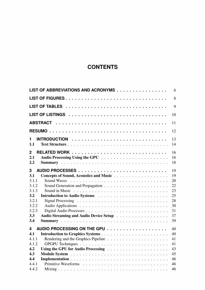
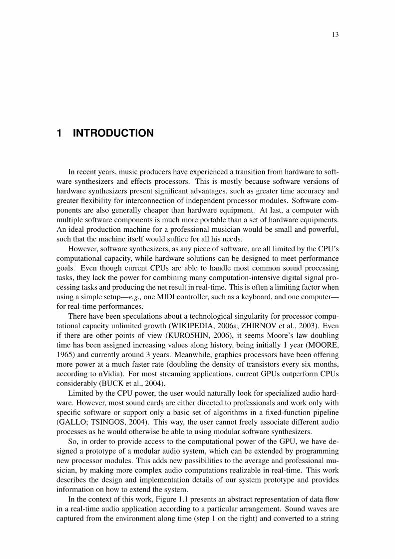
In the context of this work, Figure 1.1 presents an abstract representation of data flowin a real-time audio application according to a particular arrangement. Sound waves arecaptured from the environment along time (step 1 on the right) and converted to a string

14

AudioDevice

Mainboard

MainMemory

DataRegisters

GraphicsDevice

VideoMemory

GPU CPU

1

5234

010100011011100011...

Figure 1.1: Overview of the proposed desktop-based audio processing system.

of numbers, which is stored on the audio device (step 2). Periodically, new audio data ispassed to the CPU (step 3) which may process it directly or send it for processing on theGPU (step 4). On the next step, the audio device collects the data from the main memoryand converts it to continuous electrical signals, which are ultimately converted into airpressure waves (step 5). Up to the moment, the paths between CPU and GPU remainquite unexplored for audio processing.

In this work, we have not devised a new DSP algorithm, neither have we designed anapplication for offline audio processing1. We present a platform for audio processing onthe GPU with the following characteristics:

• Real-time results;

• Ease of extension and development of new modules;

• Advantage in terms of capabilities (e.g., polyphony, effect realism) when comparedto current CPU-based systems and possibly even hardware systems specifically de-signed for music;

• Flexible support for audio formats (i.e., any sampling rate, any number of channels);and

• Ease of integration with other pieces of software (e.g., GUIs).

We analyze some project decisions and their impact on system performance. Low-quality algorithms (i.e., those subject to noise or aliasing) have been avoided. Addition-ally, several algorithms considered basic for audio processing are implemented. We showthat the GPU performs well for certain algorithms, achieving speedups of as much as 50×or more, depending on the GPU used for comparison. The implementation is playable bya musician, which can confirm the real-time properties of the system and the quality ofthe signal, as we also discuss.

1.1 Text Structure

Chapter 2 discusses other works implementing audio algorithms on graphics hard-ware. In each case, the differences to this work are carefully addressed.1 See the difference between online and offline processing in Section 3.2.

15

Chapter 3 presents several concepts of physical sound that are relevant when process-ing audio. The basic aspects of an audio system running on a computer are presented.Topics in this chapter were chosen carefully because the digital audio processing subjectis too vast to be covered in this work. Therefore, only some methods of synthesis andeffects are explained in detail.

Next, on Chapter 4, the processes presented on the previous chapter are adapted tothe GPU and presented in full detail. We first discuss details of the operation of graphicssystems which are necessary to compute audio on them. The relationship between entitiesin the contexts of graphics and audio processing is established, and part of the source codeis presented as well.

Finally, performance comparison tests are presented and discussed on Chapter 5. Sim-ilar CPU implementations are used to establish the speedup obtained by using the GPU.The quality of the signal is also discussed, with regard to particular differences betweenarithmetic computation on CPU and GPU. Finally, the limitations of the system are ex-posed.

16

2 RELATED WORK

This chapter presents a description of some related works on using the power of theGPU for audio processing purposes. It constitutes a detailed critical review of currentwork on the subject, attempting to distinctively characterize our project from others. Wereview each work with the same concerns with which we evaluate the results of our ownwork on Chapter 5. The first section will cover 5 works more directly related to theproject. Each of them is carefully inspected under the goals established in Chapter 1. Atthe end, a short revision of the chapter is presented.

2.1 Audio Processing Using the GPU

On the short paper entitled Efficient 3D Audio Processing with the GPU, Gallo andTsingos (2004) presented a feasibility study for audio-rendering acceleration on the GPU.They focused on audio rendering for virtual environments, which requires consideringsound propagation through the medium, blocking by occluders, binaurality and Dopplereffect. In their study, they processed sound at 44.1 kHz in blocks of 1,024 samples (almost23.22 ms of audio per block) in 4 channels (each a sub-band of a mono signal) using32-bit floating-point format. Block slicing suggests that they processed audio in real-time, but the block size is large enough to cause audible delays1. They compared theperformance of implementations of their algorithm running on a 3.0 GHz Pentium 4 CPUand on an nVidia GeForce FX 5950 on AGP 8x bus. For their application, the GPUimplementation was 17% slower than the CPU implementation, but they suggested that,if texture resampling were supported by the hardware, the GPU implementation couldhave been 50% faster.

Gallo and Tsingos concluded that GPUs are adequate for audio processing and thatprobably future GPUs would present greater advantage over CPU for audio processing.They highlighted one important problem which we faced regarding IIR filters: they cannotbe implemented efficiently due to data dependency2. Unfortunately, the authors did notprovide enough implementation detail that could allow us to repeat their experiments.

Whalen (2005) discussed the use of GPU for offline audio processing of several DSPalgorithms: chorus, compression3, delay, low and highpass filters, noise gate and volumenormalization. Working with a 16-bit mono sample format, he compared the performanceof processing an audio block of 105,000 samples on a 3.0 GHz Pentium 4 CPU againstan nVidia GeForce FX 5200 through AGP.

1 See Section 3.2 for more information about latency perception. 2 See Section 4.4.5 for more infor-mation on filter implementation using the GPU. 3 In audio processing, compression refers to mappingsample amplitude values according to a shape function. Do not confuse with data compression such as inthe gzip algorithm or audio compression such as in MP3 encoding.

17

Even with such a limited setup, Whalen found up to 4 times speedups for a few al-gorithms such as delay and filtering. He also found reduced performance for other algo-rithms, and pointed out that this is due to inefficient access to textures. Since the blocksize was much bigger than the maximum size a texture may have on a single dimension,the block needed to be mapped to a 2D texture, and a slightly complicated index trans-lation scheme was necessary. Another performance factor pointed out by Whalen is thattexels were RGBA values and only the red channel was being used. This not only wastescomputation but also uses caches more inefficiently due to reduced locality of reference.

Whalen did not implement any synthesis algorithms, such as additive synthesis orfrequency modulation. Performance was evaluated for individual algorithms in a singlepass, which does not consider the impact of having multiple render passes, or changingthe active program frequently. It is not clear from the text, but probably Whalen timedeach execution including data transfer times between the CPU and the GPU. As explainedin Chapter 4, transfer times should not be counted, because transferring can occur whilethe GPU processes. Finally, Whalen’s study performs only offline processing.

Jedrzejewski and Marasek (2004) used a ray-tracing algorithm to compute an impulseresponse pattern from one sound source on highly occluded virtual environments. Eachwall of a room is assigned an absorption coefficient. Rays are propagated from the pointof the sound source up to the 10th reflection. This computation resulted in a speedup ofalmost 16 times over the CPU version. At the end, ray data was transferred to main mem-ory, leaving to the CPU the task of computing the impulse response and the reverberationeffect.

Jedrzejewski and Marasek’s work is probably very useful in some contexts—e.g., gameprogramming—, but compared to the goals of this work, it has some relevant drawbacks.First, the authors themselves declared that the CPU version of the tracing process wasnot highly optimized. Second, there was no reference to the constitution of the machineused for performance comparison. Third, and most importantly, all processing besidesraytracing is implemented on the CPU. Finally, calculation of an impulse response is aspecific detail of spatialization sound effects’ implementation.

BionicFX (2005) is the first and currently only commercial organization to announceGPU-based audio components. BionicFX is developing a DSP engine named RAVEXand a reverb processor named BionicReverb, which should run on the RAVEX engine.Although in the official home page it is claimed that those components will be released assoon as possible, the website has not been updated since at least September, 2005 (whenwe first reached it). We have tried to contact the company but received no reply. As such,we cannot evaluate any progress BionicFX has achieved up to date.

Following a more distant line, several authors have described implementations ofthe FFT algorithm on GPUs (ANSARI, 2003; SPITZER, 2003; MORELAND; ANGEL,2003; SUMANAWEERA; LIU, 2005). 1D FFT is required in some more elaborated audioalgorithms. Recently, GPUFFTW (2006), a high performance FFT library using the GPU,was released. Its developers claim that it provides a speedup factor of 4 when comparedto single-precision optimized FFT implementations on current high-end CPUs.

The reader shall note that most of the aforementioned works were released at a timewhen GPUs presented more limited capacity. That may partially justify some of the lowperformance results.

There has been unpublished scientific development on audio processing, oriented ex-clusively toward implementation on commercial systems. Since those products are animportant part of what constitutes the state of the art, you may refer to Appendix A for an

18

overview of some important commercial products and the technology they apply.In contrast to the described techniques, our method solves a different problem: the

mapping from a network model of virtually interconnected software modules to the graph-ics pipeline processing model. Our primary concern is how the data is passed from onemodule to another using only GPU operations and the management of each module’s in-ternal data4. This allows much greater flexibility to program new modules and effectivelyturns GPUs into general music production machines.

2.2 Summary

This chapter discussed the related work on the domain of GPU-based audio process-ing. None of the mentioned works is explicitly a real-time application, and the ones per-forming primitive audio algorithms report little advantage of the GPU over the CPU. Mostof them constitute test applications to examine GPU’s performance for audio processing,and the most recent one dates from more than one year ago. Therefore, the subject needsan up-to-date in-depth study.

The next chapter discusses fundamental concepts of audio and graphics systems. Theparts of the graphics processing pipeline that can be customized and rendering settingswhich must be considered to perform general purpose processing on the GPU are pre-sented. Concepts of sound and the structure of audio systems also are covered. At last,we present the algorithms we implemented in this application.

4 See Section 3.2.2 for information on architecture of audio applications.

19

3 AUDIO PROCESSES

This chapter presents basic concepts that will be necessary for understanding the de-scription of our method for processing sound on graphics hardware. The first sectionpresents definitions related with the physical and perceptual concepts of sound. The nextsections discusses audio processes from a computational perspective. These sections re-ceive more attention, since an understanding of audio processing is fundamental to under-stand what we have built on top of the graphics system and why.

3.1 Concepts of Sound, Acoustics and Music

Sound is a mechanical perturbation that propagates on a medium (typically, air) alongtime. The study of sound and its behavior is called acoustics. A physical sound field ischaracterized by the pressure level on each point of space at each instant in time. Soundgenerally propagates as waves, causing local regions of compression and rarefaction. Airparticles are, then, displaced and oscillate. This way, sound manifests as continuouswaves. Once reaching the human ear, sound waves induce movement and subsequentnervous stimulation on a very complex biological apparatus called cochlea. Stimuli arebrought by nerves to brain, which is responsible for the subjective interpretation given tosound (GUMMER, 2002). Moore (1990, p. 18) defines the basic elements of hearing as

sound waves → auditory perception → cognition

It is known since ancient human history that objects in our surroundings can producesound when they interact (normally by collision, but often also by attrition). By trans-ferring any amount of mechanical energy to an object, molecules on its surface move toa different position and, as soon as the source of energy is removed, accumulated elastictension induces the object into movement. Until the system reaches stability, it oscillatesin harmonic motion, disturbing air in its surroundings, thereby transforming the accumu-lated energy into sound waves. Properties of the object such as size and material alter thenature of elastic tension forces, causing the object’s oscillation pattern to change, leadingto different kinds of sound.

Because of that, humans have experimented with many object shapes and materials toproduce sound. Every culture developed a set of instruments with which it produces musicaccording to its standards. Before we begin defining characteristics of sound which hu-mans consider interesting, we need to understand more about the nature of sound waves.

20

3.1.1 Sound Waves

When working with sound, normally, we are interested on the pressure state at onesingle point in space along time1. This disregards the remaining dimensions, thus, soundat a point is a function only of time. Let w : R → R be a function representing a wave.w (t) represents the amplitude of the wave at time t. Being oscillatory phenomena, wavescan be divided in cycles, which are time intervals that contain exactly one oscillation. Acycle is often defined over a time range where w (t), as t increases, starts at zero, increasesinto a positive value, then changes direction, assumes negative values, and finally returnsto zero2. The period of a cycle is the difference in time between the beginning and theend of a single cycle, i.e., if the cycle starts at t0 and ends at t1, its period T is simplydefined as T = t1 − t0. The frequency of a wave is the number of cycles it presents pertime unit. The frequency f of a wave whose period is T is defined as f = N

t= 1

T, where

N represents the number of cycles during time t. The amplitude of a cycle A is defined asthe highest deviation from the average level that w achieves during the cycle. The averagelevel is mapped to amplitude zero, so the amplitude can be defined as the maximum valuefor |w (t)| with t0 ≤ t ≤ t1. Power is a useful measure of perceived intensity of the wave.Power P and amplitude A are related by A2 ∝ P . The root-mean-square (RMS) powerof wave is an useful measure in determining the wave’s perceived intensity. The RMSpower PRMS of wave f with T0 ≤ t ≤ T1 is defined as

PRMS =

√1

T1 − T0

∫ T1

T0

w (t)2 dt (3.1)

To compare the relative power of two waves, the decibel scale is often used. Given twowaves with powers P0 and P1 respectively, the ratio P1

P0can be expressed in decibels (dB)

as

PdB = 10 log10

(P1

P0

)(3.2)

Remark When the time unit is the second (s), frequency (cycles per second) is measuredin Hertz (Hz). Hertz and seconds are reciprocals, such that Hz = 1

s.

A periodic wave w is such that a single oscillation pattern repeats infinitely in theimage of w throughout its domain, i.e., there is T ∈ R such that w (t) = w (t + T ) forany t ∈ R. The minimum value of T for which this equation holds defines precisely to theperiod of the wave. No real world waves are periodic, but some can achieve a seeminglyperiodic behavior during limited time intervals. In such cases, they are called quasi-periodic. Notice, then, that amplitude, period and frequency of a wave are characteristicsthat can change along time, except for the theoretical abstraction of periodic waves3.

As all waves, sound exhibits reflection when hitting a surface, interference whenmultiple waves “crossing” the same point in space overlap, and rectilinear propagation.

1 This is a simplification that derives from the fact that microphones, loudspeakers and even the human earinteract with sound at a very limited region in space. The sound phenomenon requires a three-dimensionalfunction to be represented exactly. 2 This definition works for periodic waves, but it is very inaccuratefor most wave signals and cannot be applied in practical applications. 3 One should note that, differentlyfrom quasi-periodic signals, periodic signals present well-defined characteristics such as period, frequencyand amplitude. In this case, these characteristics are constants through all the domain.

21

Sound also experiences refraction, diffraction and dispersion, but those effects are gener-ally not interesting to audio processing because they mainly affect only sound spatializa-tion, which can be innacurately approximated considering only reflections.

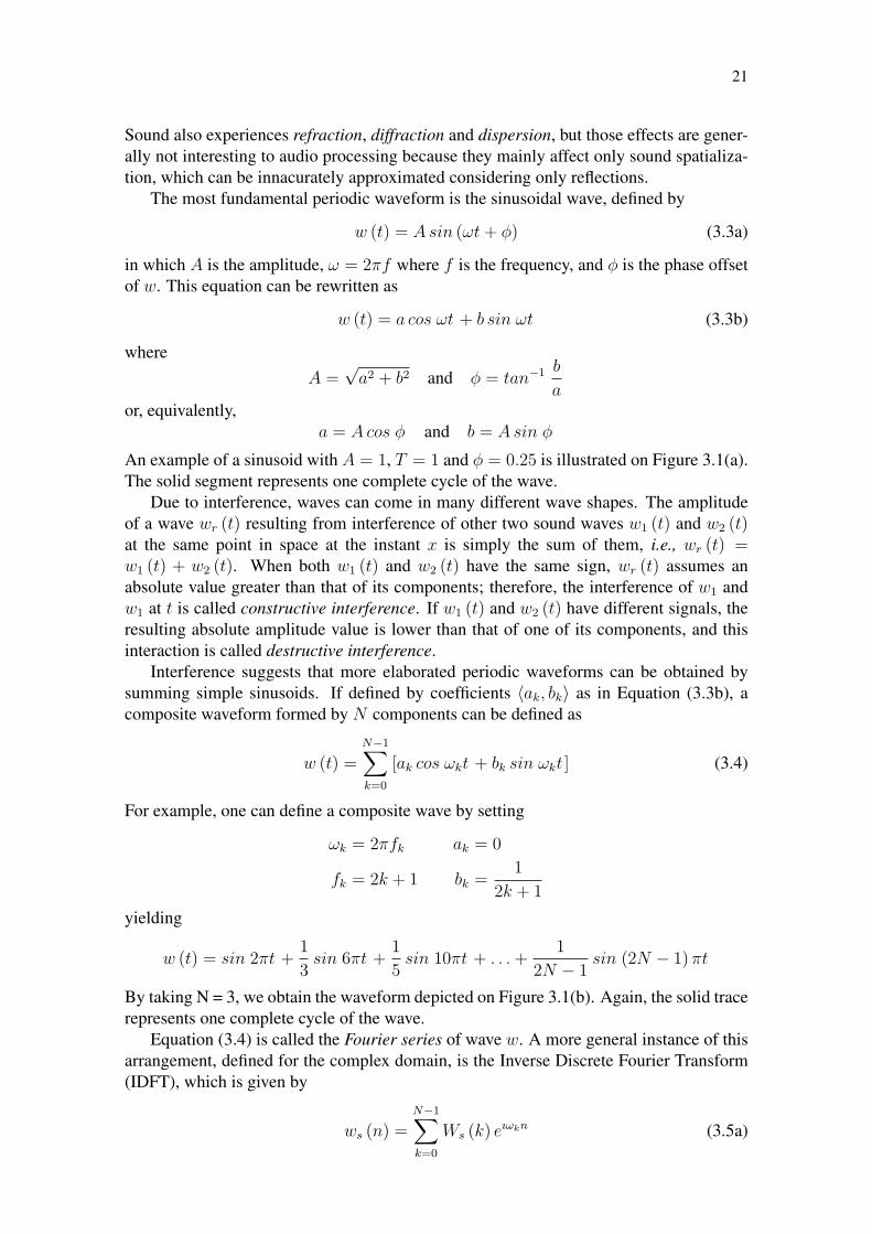
The most fundamental periodic waveform is the sinusoidal wave, defined by

w (t) = A sin (ωt + φ) (3.3a)

in which A is the amplitude, ω = 2πf where f is the frequency, and φ is the phase offsetof w. This equation can be rewritten as

w (t) = a cos ωt + b sin ωt (3.3b)

whereA =

√a2 + b2 and φ = tan−1 b

aor, equivalently,

a = A cos φ and b = A sin φ

An example of a sinusoid with A = 1, T = 1 and φ = 0.25 is illustrated on Figure 3.1(a).The solid segment represents one complete cycle of the wave.

Due to interference, waves can come in many different wave shapes. The amplitudeof a wave wr (t) resulting from interference of other two sound waves w1 (t) and w2 (t)at the same point in space at the instant x is simply the sum of them, i.e., wr (t) =w1 (t) + w2 (t). When both w1 (t) and w2 (t) have the same sign, wr (t) assumes anabsolute value greater than that of its components; therefore, the interference of w1 andw1 at t is called constructive interference. If w1 (t) and w2 (t) have different signals, theresulting absolute amplitude value is lower than that of one of its components, and thisinteraction is called destructive interference.

Interference suggests that more elaborated periodic waveforms can be obtained bysumming simple sinusoids. If defined by coefficients 〈ak, bk〉 as in Equation (3.3b), acomposite waveform formed by N components can be defined as

w (t) =N−1∑k=0

[ak cos ωkt + bk sin ωkt ] (3.4)

For example, one can define a composite wave by setting

ωk = 2πfk ak = 0

fk = 2k + 1 bk =1

2k + 1

yielding

w (t) = sin 2πt +1

3sin 6πt +

1

5sin 10πt + . . . +

1

2N − 1sin (2N − 1) πt

By taking N = 3, we obtain the waveform depicted on Figure 3.1(b). Again, the solid tracerepresents one complete cycle of the wave.

Equation (3.4) is called the Fourier series of wave w. A more general instance of thisarrangement, defined for the complex domain, is the Inverse Discrete Fourier Transform(IDFT), which is given by

ws (n) =N−1∑k=0

Ws (k) eıωkn (3.5a)

22

t

w (t)

(a) A simple sinusoidal wavewith φ = 0.25.

t

w (t)

(b) A wave composed by threesinusoids with φ = 0.

f

W (f)

1 3 5

1

31

5

(c) Real amplitude spectrum ofwaveform on item (b).

Figure 3.1: Examples of waveform composition.

where ws, Ws : Z→ C. To finally obtain values for W (k) from any periodic wave w, wecan apply the Discrete Fourier Transform (DFT), given by

Ws (k) =N−1∑n=0

ws (n) e−ıωkn (3.5b)

Ws is called the spectrum of waveform ws. Ws (k) is a vector on the complex planerepresenting the k-th component of ws. Similarly to Equation (3.3b), if Ws (k) = ak +bkı,where ı =

√−1, we can obtain the amplitude A (k) and phase φ (k) of this component

by

A (k) =√

a2k + b2

k and φ (k) = tan−1 bk

ak

(3.5c)

Given the amplitude values and the fact that A2 ∝ P , one can calculate the power spec-trum of ws, which consists of power assigned to each frequency component.

Notice that n represents the discrete time (corresponding to the continuous variable t),and k, the discrete frequency (corresponding to f ). Both DFT and IDFT can be general-ized to a continuous (real or complex) frequency domain, but this is not necessary for thiswork. Furthermore, both the DFT and the IDFT have an optimized implementation calledthe Fast Fourier Transform (FFT), for when N is a power of 2. The discrete transforms canbe extended into time-varying versions to support the concept of quasi-periodicity. Thisis done by applying the DFT to small portions of the signal instead of the full domain.

3.1.2 Sound Generation and Propagation

Recall from the beginning of this section that sound can be generated when two ob-jects touch each other. This is a particular case of resonance, in which the harmonicmovement of molecules of the object is induced when the object receives external energy,more often in the form of waves. An object can, thus, produce sound when hit, rubbed,bowed, and also when it receives sound waves. All objects, when excited, have the natu-ral tendency to oscillate more at certain frequencies, producing sound with more energyat them. Some objects produce sound where the energy distribution has clearly distinctmodes. Another way of looking at resonance is that, actually, the object absorbs energyfrom certain frequencies.

As sound propagates, it interacts with many objects in space. Air, for example, ab-sorbs some energy from it. Sound waves also interact with obstacles, suffering reflection,refraction, diffraction and dispersion. In each of those phenomena, energy from certainfrequencies is absorbed, and the phase of each component can be changed. The result

23

of this is a complex cascade effect. It is by analyzing the characteristics of the resultingsound that animals are able to locate the position of sound sources in space.

The speed at which sound propagates is sometimes important to describe certain soundphenomena. This speed determines how much delay exists between generation and per-ception of the sound. It affects, for example, the time that each reflection of the soundon the surrounding environment takes to arrive at the ear. If listener and source are mov-ing with respect to each other, the sound wave received by the listener is compressed ordilated in time domain, causing the frequency of all components to be changed. This iscalled Doppler effect and is important in the simulation of virtual environments.

3.1.3 Sound in Music

Recall from Equation (3.5c) that amplitude and phase offset can be calculated fromthe output values of the DFT for each frequency in the domain. Recall from the begin-ning of this section that the cochlea is the component of the human ear responsible forconverting sound vibration into nervous impulses. Inside the cochlea, we find the innerhair cells, which transform vibrations in the fluid (caused by sound arriving at the ear)into electric potential. Each hair cell has an appropriate shape to resonate at a specificfrequency. The potential generated by a hair cell represents the amount of energy on aspecific frequency component. However not mathematically equivalent, the informationabout energy distribution produced by the hair cells is akin to that obtained by extractingthe amplitude component from the result of a time-varying Fourier transform of the soundsignal4. Once at the brain, the electric signals are processed by a complex neural network.It is believed that this network extracts information by calculating correlationships involv-ing present and past inputs of each frequency band. Exactly how this network operatesis still not well understood. It is, though, probably organized in layers of abstraction, inwhich each layer identifies some specific characteristics of the sound being heard, beingwhat we call “attractiveness” processed at the most abstract levels—thus, the difficulty ofdefining objectively what music is.

The ear uses the spectrum information to classify sounds as harmonic or inharmonic.A harmonic sound presents high-energy components whose frequencies fk are all integermultiples of a certain number f1, which is called the fundamental frequency. In this case,components are called harmonics. The component with frequency f1 is simply referred toas the fundamental. Normally, the fundamental is the highest energy component, thoughthis is not necessary. An inharmonic sound can either present high-energy componentsat different frequencies, called partials or, in the case of noise, present no modes in theenergy distribution on the sound’s spectrum. In nature, no sound is purely harmonic,since noise is always present. When classifying sounds, then, the brain often abstractsfrom some details of the sound. For example, the sound of a flute is often characterized asharmonic, but flutes produce a considerably noisy spectrum, simply with a few strongerharmonic components. Another common example is the sound of a piano, which containspartials and is still regarded as a harmonic sound.

In music, a note denotes an articulation of an instrument to produce sound. Each notehas three basic qualities:

• Pitch, which is the cognitive perception of the fundamental frequency;

• Loudness, which is the cognitive perception of acoustic power; and4 There is still debate on the effective impact of phase offset to human sound perception. For now, weassume that the ear cannot sense phase information.

24

• Timbre or tone quality, which is the relative energy distribution of the components.Timbre is what actually distinguishes an instrument from another. Instrumentscan also be played in different expressive ways (e.g., piano, fortissimo, pizzicatto),which affects the resulting timbre as well.

The term tone may be used to refer to the pitch of the fundamental. Any componentwith higher pitch than the fundamental is named an overtone. The current more com-monly used definition for music is that “it is a form of expression through structuring oftones and silence over time” (WIKIPEDIA, 2006b). All music is constructed by placingsound events (denoted as notes) in time. Notes can be played individually or together, andthere are cultural rules to determining if a combination of pitches sound well when playedtogether or not.

Two notes are said to be consonant if they sound stable and harmonized when playedtogether. Pitch is the most important factor in determining the level of consonance. Be-cause of that, most cultures have chosen a select set of pitches to use in music. A set ofpredefined pitches is called a scale.

Suppose two notes with no components besides the fundamental frequency beingplayed together. If those tones have the same frequency, they achieve maximum con-sonance. If they have very close frequencies, but not equal, the result is a wave whoseamplitude varies in an oscillatory pattern; this effect is called beating and is often undesir-able. If one of the tones has exactly the double of the frequency of the other, this generatesthe second most consonant combination. This fact is so important that it affects all currentscale systems. In this case, the highest tone is perceived simply as a “higher version” ofthe lowest tone; they are perceived as essentially the same tone. If now the higher tonehas its frequency doubled (four times that of the lower tone), we obtain another highlyconsonant combination. Therefore, a scale is built by selecting a set of frequencies in arange [f, 2f) and then by duplicating them to lower and higher ranges, i.e., by multiply-ing them by powers of two. In other words, if S is the set of frequencies that belong tothe scale, p ∈ S and f ≤ p < 2f , then

{p× 2k | k ∈ Z

}⊂ S.

In the western musical system, the scale is built from 12 tones. To refer to those tones,we need to define a notation. An interval is a relationship, on the numbering of the scale,between two tones. Most of the time, the musician uses only 7 of these 12 tones, andintervals are measured with respect to those 7 tones. The most basic set of tones if formedby several notes (named do, re, mi, fa, sol, la, si), which are assigned short names (C, D, E,F, G, A, B, respectively). Because generally only 7 notes are used together, a tone repeatsat the 8th note in the sequence; thus, the interval between a tone and its next occurrenceis called an octave. Notes are, then, identified by both their name and a number for theiroctave. It is defined that A4 is the note whose fundamental frequency is 440 Hz. The 12thtone above A4—i.e., an octave above—is A5, whose frequency is 880 Hz. Similarly, the12th tone below A4 is A3, whose frequency is 220 Hz.

In music terminology, the interval of two adjacent tones is called a semitone. If thetones have a difference of two semitones, the interval is called a whole tone5. The other 5tones missing in this scale are named using the symbols ] (sharp) and [ (flat). ] indicatesa positive shift of one semitone, and [ indicates a negative shift of one semitone. Forexample, C]4 is the successor of C4. The established order of tones is: C, C], D, D], E, F,F], G, G], A, A], and B. C], for example, is considered equivalent to D[. Other equivalentsinclude D] and E[, G] and A[, E] and F, C[ and B. One can assign frequencies to these

5 A whole tone is referred to in common music practice by the term “tone”, but we avoid this for clearness.

25

Table 3.1: The western musical scale. Note that frequency values have been rounded.Note Names

C4 C]4 D4 D]4 E4 F4 F]4 G4 G]4 A4 A]4 B4 C5262 277 294 311 330 349 370 392 415 440 466 494 523

Note Frequencies (in Hz)

notes, as suggested in Table 3.1. Notice that the frequency for C5 is the double of thatof C4 (except for the rouding error), and that the ratio between the frequency of a noteand the frequency of its predecessor is 12

√2 ≈ 1.059463. In fact, the rest of the scale is

built considering that the tone sequence repeats and that the ratio between adjacent tonesis exactly 12

√26.

To avoid dealing with a complicated naming scheme and to simplify implementation,we can assign an index to each note on the scale. The MIDI standard, for example, definesthe index of C4 as 60, C]4 as 61, D as 62, etc. A translation between a note’s MIDI indexp and its corresponding frequency f is given by

f = 440× 2112

(p−69) and p = 69 + 12 log2

(f

440

)(3.6)

The scale system just described is called equal tempered tuning. Historically, tuningrefers to manually adjusting the tune of each note of an instrument, i.e., its perceivedfrequency. There are other tunings which are not discussed here. A conventional musictheory course would now proceed to the study the consonance of combinations of notesof different pitches on the scale and placed on time, but this is not a part of this work’sdiscussion and should be left for the performer only.

3.2 Introduction to Audio Systems

The term audio may refer to audible sound, i.e., to the components of sound signalswithin the approximate range of 20 Hz to 20 kHz, which are perceivable to the human. Ithas been used also to refer to sound transmission and to high-fidelity sound reproduction.In this text, this term is used when referring to digitally manipulated sound informationfor the purpose of listening.

To work with digital audio, one needs a representation for sound. The most usualway of representing a sound signal in a computer is by storing amplitude values on anunidimensional array. This is called a digital signal, since it represents discrete ampli-tude values assigned to a discrete time domain. These values can be computed using aformula, such as Equation (3.4) or one of the formulas on Table 3.2. They can also beobtained by sampling the voltage level generated by an external transducer, such as a mi-crophone. Another transducer can be used to convert back digital signals into continuoussignals. Figure 1.1 illustrates both kinds of conversion. Alternatively, samples can alsobe recorded on digital media and loaded when needed.

Sounds can be sampled and played back from one or more points in space at thesame time. Therefore, a digital signal has three main attributes: sampling rate, sampleformat and number of channels. The samples can be organized in the array in differentarrangements. Normally, samples from the same channel are kept in consecutive posi-tions. Sometimes, each channel can be represented by an individual array. However, it is6 This scale is called equal tempered scale, and it attempts to approximate the classical Ptolemaeus scalebuilt using fractional ratios between tones.

26

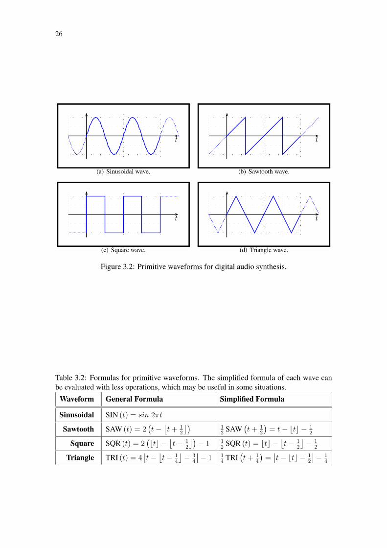
t

(a) Sinusoidal wave.

t

(b) Sawtooth wave.

t

(c) Square wave.

t

(d) Triangle wave.

Figure 3.2: Primitive waveforms for digital audio synthesis.

Table 3.2: Formulas for primitive waveforms. The simplified formula of each wave canbe evaluated with less operations, which may be useful in some situations.

Waveform General Formula Simplified Formula

Sinusoidal SIN (t) = sin 2πt

Sawtooth SAW (t) = 2(t−

⌊t + 1

2

⌋)12

SAW(t + 1

2

)= t− btc − 1

2

Square SQR (t) = 2(btc −

⌊t− 1

2

⌋)− 1 1

2SQR (t) = btc −

⌊t− 1

2

⌋− 1

2

Triangle TRI (t) = 4∣∣t− ⌊

t− 14

⌋− 3

4

∣∣− 1 14

TRI(t + 1

4

)=

∣∣t− btc − 12

∣∣− 14

27

possible to merge samples from all channels in a single array by interleaving the samplesof each channel.

Any arithmetic operation can be performed on a signal stored on an array. Moreelaborate operations are generally devised to work with the data without any feedbackto the user until completion. This is called offline audio processing, and it is easy towork with. In online processing, the results of computation are supposed to be heardimmediately. But in real applications, there is a slight time delay, since any computationtakes time and the data need to be routed through components of the system until they arefinally transduced into sound waves. A more adequate term to characterize such a systemis real time, which means that the results of computation have a limited amount of timeto be completed.

To perform audio processing in real time, though, instead of working with the fullarray of samples, we need to work with parts of it. Ideally, a sample value should betransduced as soon as it becomes available, but this leads to high manufacturing costs ofaudio devices and imposes some restrictions to software implementation (since computa-tion time may vary depending on the program being executed, it may require executing ahigh amount of instructions). This is, though, a problem that affects any real-time audiosystem. If the required sample value is not available at the time it should be transduced,another value will need to be used instead of it, producing a sound different from whatwas originally intended. The value used for filling gaps is usually zero. What happenswhen a smooth waveform abruptly changes to a constant zero level is the insertion ofmany high-frequency components into the signal. The resulting sound has generally anoisy and undesired “click”7. This occurrence is referred to as an audio glitch. In orderto prevent glitches from happening, samples are stored on a temporary buffer before be-ing played. Normally, buffers are divided in blocks, and a scheme of buffer swapping isimplemented. While one block is being played, one or more blocks are being computedand queued to be played later.

The latency of a system is the time interval between an event in the inputs of thesystem and the corresponding event in the outputs. For some systems (such as an audiosystem), latency is a constant determined by the sum of latencies of each system com-ponent through which data is processed. From the point of view of the listener, latencyis the time between a controller change (such as key being touched by the performer)and the corresponding perceived change (such as the wave of a piano string reaching theperformer’s ears). Perceived latency also includes the time of sound propagation fromthe speaker to the listener and the time for a control signal to propagate through the cir-cuitry to the inputs of the audio system. On a multi-threaded system, latency is variablyaffected by race conditions and thread scheduling delays, which are unpredictable but canbe minimized by changing thread and process priorities.

It is widely accepted that real-time audio systems should present latencies of around10 ms or less. The latency L introduced by a buffered audio application is given by

L = number of buffers × samples per buffer blocksamples per time unit

(3.7)

Many physical devices, named controllers, have been developed to “play” an elec-tronic instrument. The most common device is a musical keyboard, in which keys trig-ger the generation of events. On a software application, events are normally processed7 Note, however, that the square wave on Figure 3.2(c) is formed basically of abrupt changes and still isharmonic—this is formally explained because the abrupt changes occur in a periodic manner. Its spectrum,though, presents very intense high-frequency components.

28

through a message-driven mechanism. The attributes given to each type of event arealso application-dependent and vary across different controllers and audio processing sys-tems. The maximum number of simultaneous notes that a real-time audio system can pro-cess without generating audio glitches (or without any other design limitation) is calledpolyphony. In software applications, polyphony can be logically unrestricted, limited onlyby the the processor’s computational capacity. Vintage analog instruments8 often had apolyphony of a single note (also called monophony), although some of them, such as theHammond organ, have full polyphony.

3.2.1 Signal Processing

3.2.1.1 Sampling and Aliasing

In a digital signal, samples represent amplitude values of an underlying continuouswave. Let n ∈ N be the index of a sample of amplitude ws (n). The time differencebetween samples n + 1 and n is a constant and is called sample period. The number ofsamples per time unit is the sample frequency or sampling rate.

The sampling theorem states that a digital signal sampled at a rate of R can onlycontain components whose frequencies are at most R

2. This comes from the fact that a

component of frequency exactly R2

requires two samples per cycle to represent both thepositive and the negative oscillation. An attempt of representing a component of higherfrequencies results in a reflected component of frequency below R

2. The theorem is also

known as the Nyquist theorem and R2

is called the Nyquist rate. The substitution of acomponent by another at lower frequency is called aliasing. Aliasing may be generatedby any sampling process, regardless of the kind of source audio data (analog or digital).Substituted components constitute what is called artifacts, i.e., audible and undesiredeffects (insertion or removal of components) resulting from processing audio digitally.

Therefore, any sampled sound must be first processed to remove energy from com-ponents above the Nyquist rate. This is performed using an analog low-pass filter. Thistheorem also determines the sampling rate at which real sound signals must be sampled.Given that humans can hear up to about 20 kHz, the sampling rate must be of at least40 kHz to represent the highest perceivable frequency. However, frequencies close to20 kHz are not represented well enough. It is observed that those frequencies present anundesired beating pattern. For that reason, most sampling is performed with samplingrates slightly above 40 kHz. The sampling rate of audio stored on a CD, for example,is 44.1 kHz. Professional audio devices usually employ a sampling rate of 48 kHz. Itis possible, though, to use any sampling rate, and some professionals have worked withsampling rates as high as 192 kHz or more, because, with that, some of the computationperformed on audio signals is more accurate.

When the value of a sample ws (n) is obtained for an underlying continuous wavew at time t, it is rounded to the nearest digital representation of w (t). The differencebetween ws (n) and w (t) is called the quantization error, since the values of w (t) areactually quantized to the nearest values. Therefore, ws (n) = w (t (n)) + ξ (n), whereξ is the error signal. This error signal is characterized by many abrupt transitions andthus, as we have seen, is rich in high-frequency components, which are easy to perceive.When designing an audio system, it is important to choose an adequate sample formatto reduce the quantization error to an imperceptible level. The RMS of ξ is calculatedusing Equation (3.1). The ratio between the power of the loudest representable signal and8 An analog instrument is an electric device that processes sound using components that transform contin-uous electric current instead of digital microprocessors.

29

the power of ξ, expressed in decibels according to Equation (3.2), is called the signal-to-quantization-error-noise ratio (SQNR). Usual sampling rates with a high SQNR are16, 24 or 32-bit integer, 32 or 64-bit floating point. The sample format of audio storedon a CD, for example, is 16-bit integer. There are alternative quantization schemes, suchas logarithmic quantization (the sample values are actually the logarithm of their originalvalues), but the floating point representation usually presents the same set of features.

Analog-to-Digital Converters (ADC) and Digital-to-Analog Converters (DAC) aretransducers9 used to convert between continuous and discrete sound signals. These com-ponents actually convert between electric representations, and the final transduction intosound is performed by another device, such as a loudspeaker. Both DACs and ADCs mustimplement analog filters to prevent the aliasing effects caused by sampling.

3.2.1.2 Signal Format

Common possible representations of a signal are classified as:

• Pulse coded modulation (PCM), which corresponds to the definition of audio wehave presented. The sample values of a PCM signal can represent

– linear amplitude;

– non-linear amplitude, in which amplitude values are mapped to a differentscale (e.g., in logarithmic quantization); and

– differential of amplitude, in which, instead of the actual amplitude, the differ-ence between two consecutive sample’s amplitude is stored.

• Pulse density modulation (PDM), in which the local density of a train of pulses(values of 0 and 1 only) determines the actual amplitude of the wave, which isobtained after the signal is passed through an analog low-pass filter;

• Lossy compression, in which part of the sound information (generally componentswhich are believed not to be perceptible) is removed before data compression; and

• Lossless compression, in which all the original information is preserved after datacompression.

Most audio applications use the PCM linear format because digital signal processingtheory—which is based on continuous wave representations in time—generally can beapplied directly without needing to adapt formulas from the theory. To work with otherrepresentations, one would often need, while processing, to convert sample values to aPCM linear format, perform the operation, and then convert the values back to the workingformat.

Common PCM formats used to store a single sound are:

• CD audio: 44.1 kHz, 16-bit integer, 2 channels (stereo);

• DVD audio: 48–96 kHz, 24-bit integer, 6 channels (5.1 surround); and

• High-end studios: 192–768 kHz, 32–64-bit floating point, 2–8 channels.

9 A transducer is a device used to convert between different energy types.

30

The bandwidth (the number of bytes per time unit) expresses the computational trans-fer speed requirements for audio processing according to the sample format. A signalbeing processed continuously or transferred is a type of data stream. Considering uncom-pressed formats only, the bandwidth B of a sound stream of sampling rate R, sample sizeS and number of channels C is obtained by B = RSC. For example, streaming CD au-dio takes a bandwidth of 176.4 kBps, and a sound stream with sampling rate of 192 kHz,sample format of 64-bit and 8 channels has a bandwidth of 12,288 kBps (12 MBps).

3.2.2 Audio Applications

The structure of major audio applications varies widely, depending on their purpose.Among others, the main categories include:

• Media players, used simply to route audio data from its source (a hard disk, forexample) to the audio device. Most media players also offer basic DSPs (digitalsignal processors), such as equalizers, presented to the user on a simplified graphi-cal interface that does not permit customizing the processing model (e.g., the orderin which DSPs are applied to the audio);

• Scorewriters, used to typeset song scores on a computer. Most scorewriters canconvert a score to MIDI and play the MIDI events. Done this way, the final MIDIfile generally does not include much expressivity (though there has been work togenerate expressivity automatically (ISHIKAWA et al., 2000)) and is normally notsuitable for professional results;

• Trackers and sequencers, used to store and organize events and samples that com-pose a song. This class of application is more flexible than scorewriters, since theyallow full control over the generation of sound; and

• Plug-in-based applications, in which computation is divided in software pieces,named modules or units, that can be integrated on the main application, responsiblefor routing signals between modules.

Some audio applications present characteristics belonging to more than one category(e.g., digital audio workstations include a tracker and/or a sequencer and are based ona plug-in architecture). Plug-in based applications are usually the most interesting for aprofessional music producer, since it can be extended with modules from any externalsource.

3.2.2.1 Modular Architecture

The idea behind a modular architecture is to model in software the interconnection ofprocessing units, similar to the interconnection of audio equipment with physical cables.A module is composed of inputs, outputs and a processing routine. The main advantagesof a modular architecture are that computation is encapsulated by modules and that theirresults can be easily combined simply by defining the interconnection between modules,which can be done graphically by the user.

The processing model is a directed acyclic graph which models an unidirectional net-work of communication between modules. Figure 3.3 presents an example of a processingmodel on a modular architecture that a user can generate graphically. Each module hasa set of input and output slots, depicted as small numbered boxes. Modules A and B arenamed generators, since they only generate audio signals, having no audio inputs. C, D

31

A

B

C

D

E

F

1

12

1

123

1

12

12 1

1

Figure 3.3: Graphical representation of a processing model on a modular architecture.A, B, C, D, E and F are modules. Numbered small boxes represent the input and outputslots of each module. The arrows represent how inputs and outputs of each module areconnected, indicating how sound samples are passed among module programs.

and E are named effects, since they operate on inputs and produce output signals withthe intent of changing some characteristic of the input sound—e.g., energy distribution ofcomponents, in the case of an equalizer effect. F is a representation of the audio deviceused to play the resulting sound wave. Each module can receive controller events, whichare used to change the value of parameters used for computation. A generator also usesevents to determine when a note begins and stops playing.

On Figure 3.3, the signals arriving at module F are actually implicitly mixed beforebeing assigned to the single input slot. Recall from Section 3.1.1 that the interference ofmultiple waves at time t produces a wave resulting from the sum of the amplitudes of allinteracting waves at time t at the same point. For that reason, mixing consists of summingcorresponding samples from each signal. Other operations could be made implicit aswell, such as, for example, signal format conversion. Another important operation (notpresent on the figure) is gain which scales the amplitude of the signal by a constant,thus altering its perceived loudness. One may define that each input implicitly adds again parameter to the module parameter set. Together, gain and mixing are the mostfundamental operations in multi-track recording, in which individual tracks of a piece arerecorded and then mixed, each with a different amount of gain applied to. This allowsbalancing the volume across all tracks.

Remark On a more general case, the processing model shown in Figure 3.3 could alsoinclude other kinds of streams and modules, such as video and subtitle processors. How-ever, the implementation of the modular system becomes significantly more complex withthe addition of certain features.

3.2.3 Digital Audio Processes

In this section, several simple but frequently used audio processes are presented.These algorithms were selected to discuss how they can be implemented on the GPU10.More information about audio processes can be found at TOLONEN; VÄLIMÄKI; KAR-JALAINEN (1998). In the following subsections, n represents the index of the “current”sample being evaluated, x is the input vector and y is the output vector. x (n) refers to thesample at position n in x and is equivalently denoted as xn on the following figures, forclarity.10 See Section 4.4.

32

OutputsInputs

IIRFIR

xnxn-1xn-2xn-3

a0a1a2a3 b1 b2

yn-1 yn-2yn

××××∑

××

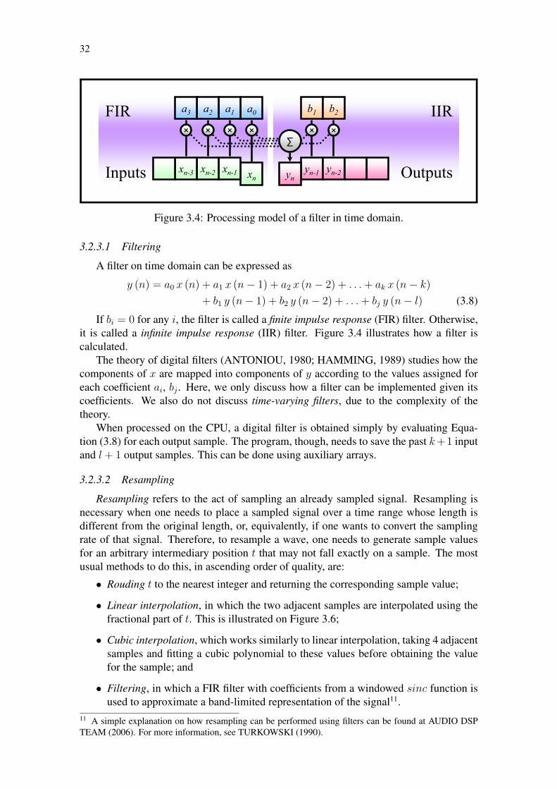
Figure 3.4: Processing model of a filter in time domain.

3.2.3.1 Filtering

A filter on time domain can be expressed as

y (n) = a0 x (n) + a1 x (n− 1) + a2 x (n− 2) + . . . + ak x (n− k)

+ b1 y (n− 1) + b2 y (n− 2) + . . . + bj y (n− l) (3.8)

If bi = 0 for any i, the filter is called a finite impulse response (FIR) filter. Otherwise,it is called a infinite impulse response (IIR) filter. Figure 3.4 illustrates how a filter iscalculated.

The theory of digital filters (ANTONIOU, 1980; HAMMING, 1989) studies how thecomponents of x are mapped into components of y according to the values assigned foreach coefficient ai, bj . Here, we only discuss how a filter can be implemented given itscoefficients. We also do not discuss time-varying filters, due to the complexity of thetheory.

When processed on the CPU, a digital filter is obtained simply by evaluating Equa-tion (3.8) for each output sample. The program, though, needs to save the past k +1 inputand l + 1 output samples. This can be done using auxiliary arrays.

3.2.3.2 Resampling

Resampling refers to the act of sampling an already sampled signal. Resampling isnecessary when one needs to place a sampled signal over a time range whose length isdifferent from the original length, or, equivalently, if one wants to convert the samplingrate of that signal. Therefore, to resample a wave, one needs to generate sample valuesfor an arbitrary intermediary position t that may not fall exactly on a sample. The mostusual methods to do this, in ascending order of quality, are:

• Rouding t to the nearest integer and returning the corresponding sample value;

• Linear interpolation, in which the two adjacent samples are interpolated using thefractional part of t. This is illustrated on Figure 3.6;

• Cubic interpolation, which works similarly to linear interpolation, taking 4 adjacentsamples and fitting a cubic polynomial to these values before obtaining the valuefor the sample; and

• Filtering, in which a FIR filter with coefficients from a windowed sinc function isused to approximate a band-limited representation of the signal11.

11 A simple explanation on how resampling can be performed using filters can be found at AUDIO DSPTEAM (2006). For more information, see TURKOWSKI (1990).

33

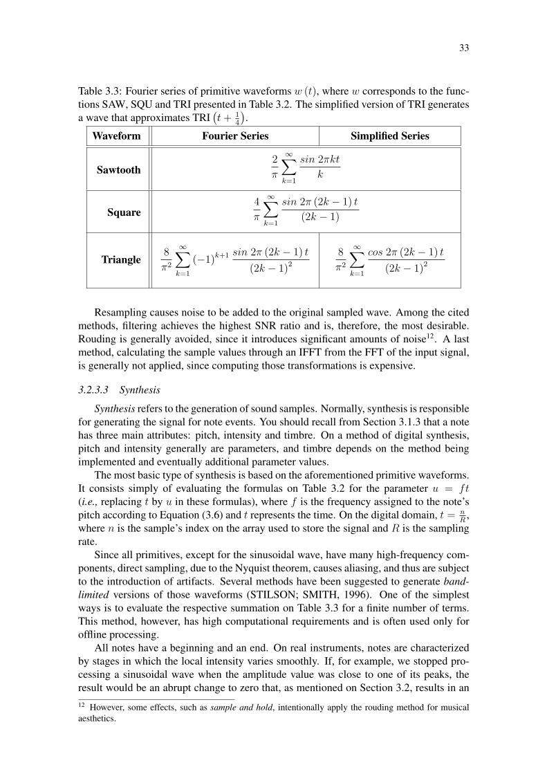
Table 3.3: Fourier series of primitive waveforms w (t), where w corresponds to the func-tions SAW, SQU and TRI presented in Table 3.2. The simplified version of TRI generatesa wave that approximates TRI

(t + 1

4

).

Waveform Fourier Series Simplified Series

Sawtooth2

π

∞∑k=1

sin 2πkt

k

Square4

π

∞∑k=1

sin 2π (2k − 1) t

(2k − 1)

Triangle8

π2

∞∑k=1

(−1)k+1 sin 2π (2k − 1) t

(2k − 1)2

8

π2

∞∑k=1

cos 2π (2k − 1) t

(2k − 1)2

Resampling causes noise to be added to the original sampled wave. Among the citedmethods, filtering achieves the highest SNR ratio and is, therefore, the most desirable.Rouding is generally avoided, since it introduces significant amounts of noise12. A lastmethod, calculating the sample values through an IFFT from the FFT of the input signal,is generally not applied, since computing those transformations is expensive.

3.2.3.3 Synthesis

Synthesis refers to the generation of sound samples. Normally, synthesis is responsiblefor generating the signal for note events. You should recall from Section 3.1.3 that a notehas three main attributes: pitch, intensity and timbre. On a method of digital synthesis,pitch and intensity generally are parameters, and timbre depends on the method beingimplemented and eventually additional parameter values.

The most basic type of synthesis is based on the aforementioned primitive waveforms.It consists simply of evaluating the formulas on Table 3.2 for the parameter u = ft(i.e., replacing t by u in these formulas), where f is the frequency assigned to the note’spitch according to Equation (3.6) and t represents the time. On the digital domain, t = n

R,

where n is the sample’s index on the array used to store the signal and R is the samplingrate.

Since all primitives, except for the sinusoidal wave, have many high-frequency com-ponents, direct sampling, due to the Nyquist theorem, causes aliasing, and thus are subjectto the introduction of artifacts. Several methods have been suggested to generate band-limited versions of those waveforms (STILSON; SMITH, 1996). One of the simplestways is to evaluate the respective summation on Table 3.3 for a finite number of terms.This method, however, has high computational requirements and is often used only foroffline processing.

All notes have a beginning and an end. On real instruments, notes are characterizedby stages in which the local intensity varies smoothly. If, for example, we stopped pro-cessing a sinusoidal wave when the amplitude value was close to one of its peaks, theresult would be an abrupt change to zero that, as mentioned on Section 3.2, results in an12 However, some effects, such as sample and hold, intentionally apply the rouding method for musicalaesthetics.

34

A D S R

0 1 3 9.5 12.5

0.4

+1

-1

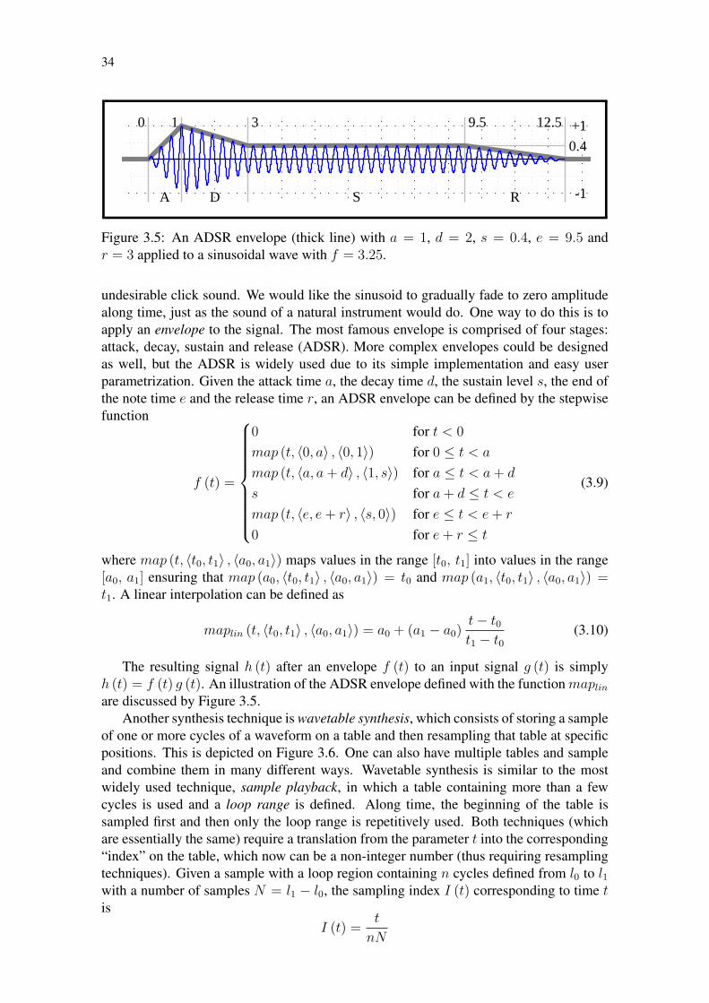
Figure 3.5: An ADSR envelope (thick line) with a = 1, d = 2, s = 0.4, e = 9.5 andr = 3 applied to a sinusoidal wave with f = 3.25.

undesirable click sound. We would like the sinusoid to gradually fade to zero amplitudealong time, just as the sound of a natural instrument would do. One way to do this is toapply an envelope to the signal. The most famous envelope is comprised of four stages:attack, decay, sustain and release (ADSR). More complex envelopes could be designedas well, but the ADSR is widely used due to its simple implementation and easy userparametrization. Given the attack time a, the decay time d, the sustain level s, the end ofthe note time e and the release time r, an ADSR envelope can be defined by the stepwisefunction

f (t) =

0 for t < 0

map (t, 〈0, a〉 , 〈0, 1〉) for 0 ≤ t < a

map (t, 〈a, a + d〉 , 〈1, s〉) for a ≤ t < a + d

s for a + d ≤ t < e

map (t, 〈e, e + r〉 , 〈s, 0〉) for e ≤ t < e + r

0 for e + r ≤ t

(3.9)

where map (t, 〈t0, t1〉 , 〈a0, a1〉) maps values in the range [t0, t1] into values in the range[a0, a1] ensuring that map (a0, 〈t0, t1〉 , 〈a0, a1〉) = t0 and map (a1, 〈t0, t1〉 , 〈a0, a1〉) =t1. A linear interpolation can be defined as

maplin (t, 〈t0, t1〉 , 〈a0, a1〉) = a0 + (a1 − a0)t− t0t1 − t0

(3.10)

The resulting signal h (t) after an envelope f (t) to an input signal g (t) is simplyh (t) = f (t) g (t). An illustration of the ADSR envelope defined with the function maplin

are discussed by Figure 3.5.Another synthesis technique is wavetable synthesis, which consists of storing a sample

of one or more cycles of a waveform on a table and then resampling that table at specificpositions. This is depicted on Figure 3.6. One can also have multiple tables and sampleand combine them in many different ways. Wavetable synthesis is similar to the mostwidely used technique, sample playback, in which a table containing more than a fewcycles is used and a loop range is defined. Along time, the beginning of the table issampled first and then only the loop range is repetitively used. Both techniques (whichare essentially the same) require a translation from the parameter t into the corresponding“index” on the table, which now can be a non-integer number (thus requiring resamplingtechniques). Given a sample with a loop region containing n cycles defined from l0 to l1with a number of samples N = l1 − l0, the sampling index I (t) corresponding to time tis

I (t) =t

nN

35

Outputs

Wave

Table

ynyn-1 yn-2

× ×

+

1 - α α

α

Figure 3.6: Illustration of linear interpolation on wavetable synthesis. f represents thefractional part of the access coordinate.

Before accessing a sample, an integer index i must be mapped to fall within a valid rangeinto the sample, according to the access function

S (i) =

{i for i < l1

l0 + [(i− l1) mod N ] for i ≥ l1

which, in the case of wavetable synthesis, simplifies to S (i) = i mod N . Performingwavetable synthesis, then, requires the following steps:

• Calculate the sampling index I (u) for the input parameter u. If f is a constant, thenu = ft and f can be obtained from Equation (3.6);

• For each sample i adjacent to I (u), calculate the access index S (i); and

• Interpolate using the values from positions in the neighborhood of S (i) in the array.

After resampling, an envelope may be applied to the sample values in the same wayit was applied to the primitive waveforms, as previously discussed. Advanced wavetabletechniques can be found in BRISTOW-JOHNSON (1996).

The most general synthesis technique is additive synthesis, which consists of sum-ming sinusoidal components, similar to computing the Fourier series of a signal. Mostof the time, chosen components are harmonics of the frequency of the playing note, butthis is not required. In the simplest case, when the amplitude of components is not modu-lated by any envelope, additive synthesis is equivalent to wavetable synthesis (BRISTOW-JOHNSON, 1996, p. 4). In practice, though, an individual envelope is applied to eachcomponent. Since many components may be present, it is usual to extract parameters foreach individual envelope using data reduction techniques.

The idea of producing complex sounds from an array of simpler sounds applies notonly to sinusoidal waves. Components can be generated with any synthesis method andsummed together by applying different gains to each signal. For example, additive synthe-sis is often imitated with wavetable synthesis by summing the output of several waveta-bles and applying individual envelopes. When dealing with a set of components, one canform groups and control each group individually—for example, instead of applying oneenvelope to each component, one may apply an envelope to groups of components.

Instead of summing components, one can also start with a complex waveform—i.e., asawtooth wave—and remove components from it, usually by filtering. This is called

36

(a) I = 2 (b) I = 4 (c) I = 8

Figure 3.7: Examples of FM waveforms with fm = fc = 1.

subtractive synthesis and it is the main method used for physical modelling, the simulationof sound produced by real-world sound sources and its interaction with nearby objects.

The previously mentioned parameter u can be understood as a variable that is incre-mented from sample to sample. Though the time parameter t varies, by definition, as aconstant between any two adjacent samples, the frequency parameter may change. Thisway, u can be redefined as u (t) =

∫f (t) dt, where f (t) is the frequency at time t.

This is called frequency modulation (FM). FM synthesis is usually applied to synthesizebell and brass-like sounds. f (t) is the modulator, which is usually a sinusoidal functionmultiplied by an amplitude parameter. The function to which u is applied is the carrier,which is also usually a sinusoid. In the case where sinusoids are used for both carrier andmodulator, an FM wave can defined as

w (t) = A sin (2πfct + I sin (2πfmt)) (3.11)

The index of modulation I is defined as I = ∆ffm

, where ∆f is the amount of frequencydeviation. Higher values of I cause the distribution of energy on high-frequency compo-nents to increase. The index of harmonicity H is defined as H = fm

fc. Whenever H = 1

N

or H = N for any N ∈ N and N ≥ 1, the resulting waveform is harmonic with its fun-damental at min {fc, fm}. If I and H are both small but non-null, the result is a vibrattoeffect. However, as N grows close to 1, the harmonic content of the sinusoid starts tochange noticeably, as well as its waveform. Figure 3.7 presents several waveforms gen-erated by frequency modulation. This technique can be expanded by defining f (t) as anFM function itself. This way, one may recursively generate any level of modulation. Theharmonic content of an FM wave is the subject of a complicated theory whose discussionis beyond the scope of this work.

Sometimes it is necessary to synthesize noise too. There are many kinds of noises, butmost can be obtained from white noise, which is characterized by an uniform distributionof energy along the spectrum. For example, pink noise (energy distributed uniformlyon a logarithmic domain) can be approximated using well designed low-pass filters overa white noise input or, as done by the Csound language, using sample and hold. Anideal pseudo-random number generator, such as those implemented in most programminglibraries provided with compilers, generates white noise.

At last, granular synthesis consists of mixing along time many small sound unitsnamed granule. A granule is simply a signal which often, but not necessarily, has smalllength (around 50 ms) and smooth amplitude variation, fading to zero at the edges of thegranule. The number of different granules, size, frequency of resampling and the densityof placement along time are variable parameters. Given that the number of granules isnormally too large to be handled by a human, the study of granular synthesis focuses on

37

methods of controlling the choice of granules and their parameters more automatically.There are numerous variations and combinations of the methods described on this

subsection, and other methods, such as formant synthesis, phase distortion, etc. There arealso specific usages of the described methods for generating percussive sounds.

3.2.3.4 Effects

In this section, two simple and similar effects used frequently for music productionare described. A tap delay or simply a delay is such that of a repetition (tap) of someinput sound is produced on the output after its first occurrence. A delay effect may havemultiple taps, such that several repetitions of an input sound will be produced on futureoutputs. It can be defined as

y (n) = gw x (n) + g0 x (n− k0) + g1 x (n− k1) + . . . + gN x (n− kN)

where gw represents the wet gain—the amount of current input signal that will be imme-diately present on the output—, g0, g1 . . . , gn are the gains respective to each tap, andk0, k1 . . . , kN are the sample-positional delays of each tap. In general, the delays are ofmore than 100 ms for the delayed repetition to be perceived as a repetition instead of partof the original sound.

A similar effect is an echo, which consists of an infinite repetition of any sound thatcomes into the input. An echo can be defined as

y (n) = gw x (n) + gf y (n− k)

where gf represents the feedback gain—the change applied to the volume of a past outputsignal at its next repetition—and k is the time delay between two successive echoes.Generally, successive repetitions fade out as they repeat. This behavior can be obtainedby enforcing |f | < 1. Setting either of the constants gw or gf to a negative value causesan inversion of the signal being multiplied with the respective constant, which generallydoes not produce any audible difference13. Notice that a delay and an echo effect areactually a FIR and an IIR filter, respectively. A 1-tap delay and an echo are depictedon Figure 3.8. More complicated delay schemes can be designed, such as cross-delays(between channels) and multi-tap feedback delays. On a more general case, the delaytimes k may be substituted by non-integer values, thus requiring resampling of the signalto generate taps.

There are many other effects that are not described in this work. For instance, animportant effect is reverberation, in which multiple echoes with varying delay are applied;filtering is also often applied to simulate energy absorption by objects of an environment.Chorus, flanging, sample and hold, ring modulation, resynthesis, gapping, noise gating,etc. are other interesting audio processes.

3.3 Audio Streaming and Audio Device Setup

As discussed in Section 3.2, processing audio in real time requires the audio datato be divided in blocks. Generally, for simplicity, all blocks have a fixed amount ofsamples. After properly loaded, the driver periodically requests a block of audio from the13 An inversion of amplitude corresponds to a shift of π on each component. When two components ofsame frequency but phases with a distance of π are summed, they cancel each other (this is a destructiveinterference). Thus, in some cases, inverting the signal may produce audible effects.

38

xn-k

yn-k

gf×gf

×gw×

+

ynyn-1yn-2

xn...

...

Delay?Echo?

Figure 3.8: Combined illustration of a 1-delay and an echo effect. The input for the sumchanges according to the effect one wants to implement: for the delay, it is gf xn−k; forthe echo effect, it is gf yn−k.

application, providing or not an input block with samples that have been recorded fromthe device’s input channels in the previous step. For a continuous output, the applicationis given a certain amount of time to compute samples and provide the requested block tothe audio device.

If this computation takes longer than the given time, the behavior of the audio device isunspecified14, but if one wishes to define what is played by the sound card if this happens,a possible solution is by doing the following:

• Create an intermediary buffer containing at least two blocks of samples;

• Create a thread to fill this buffer;

• Create a semaphore for the CPU to determine when the thread should write a blockwith the data being generated, i.e., after being copied into an output block duringone execution of the callback procedure; and

• Access this buffer from the callback procedure to retrieve one completely computedblock, if necessary.

If more than two blocks are stored in the intermediary buffer, this procedure willbuffer data ahead and increase the tolerance of the system against the occurrence of audioglitches due to heavy computation. This is a typical producer-consumer problem, wherethe created thread produces blocks of audio data, which are consumed by the audio driverthrough the callback procedure. In our implementation, if a block is not ready, the audiodriver receives a block filled with silence.

As explained in Section 3.2, the format of audio contained in a block is defined byits sampling rate, sample format, number of channels and whether the data is interlievedor not. The available combinations of those characteristics vary depending on the audiodevice, driver and the API used to access the driver. A problem arises when one triesto run an application using an unsupported audio format. One may implement a pro-gram using many different formats and then choose the one supported by the device, orhe/she may also convert the audio format prior to playback. Though not all, several li-braries provide automatic audio format conversion to a certain extent. We have chosen to14 It seems acceptable that sound cards will play again the last completely computed block or simplysilence. In both cases, though, there is a high chance that an abrupt change in amplitude will happen at thetransition following the last sample of that block, causing an undesired glitch.

39

CPU SoundCardGPU primitives

1122

Figure 3.9: Illustration of the audio “pipeline”. Audio streaming is performed on step 1,and processing on the GPU is performed on step 2.

work with RtAudio (SCAVONE, 2005), which offers interesting programming options—e.g., providing audio through blocking calls instead of a callback procedure—, is portableand supports, on Microsoft Windows, the ASIO (STEINBERG, 2006) and DirectSound(MICROSOFT, 2006a) interfaces. RtAudio can convert the sample format and the in-terlieving of data as necessary, but sampling rate and number of channels still must bedetermined properly by the application.

Figure 3.9 the whole process of real-time audio processing. Audio streaming takesplace on step 1, while processing on the CPU or the GPU takes place on step 2. Thesquare blocks between each device represent the exchanged sample buffers. As we discussin Section 4.3, the CPU must also handle input from control devices such as keyboards,which are used by the musician to play a music piece.

Before we define the internal operations performed by the producer thread, we need toexplain how graphics systems work and define how to prepare them for audio processing.

3.4 Summary

This chapter presented many concepts involved in audio processing. It discussed theunderlying physical concepts of sound, mentioned how sound behaves in environmentswhich humans are used to, and presented how sound is organized in music and how acomputer system can be used to produce music. At last, we presented some of the mostfundamental sound processing algorithms.

Now all the theoretical tools necessary to start building computer systems for musicproduction have been provided. The reader should be able to visualize (at least abstractly)how to implement those algorithms. The next chapter discusses the implementation of amodular system that facilitates the development of new modules that take advantage ofthe graphics hardware.

40

4 AUDIO PROCESSING ON THE GPU

In the previous chapter, we discussed the basic concepts of physical sound and ofaudio processing on a computer. The definition of several audio processing algorithmswere given, and guidelines for the interaction with an audio device driver were given. Inthis chapter, a study of how graphics processing systems can be used to implement thegiven algorithms is presented. We present a real-time application in which sample valuesare obtained using fragment programs.

The first section of this chapter presents an “audio pipeline”, describing which com-putation needs to be executed at each step of audio processing. Then, graphics processingis described as it is usually performed today with high-end graphics hardware. The rela-tionship between entities in the contexts of graphics and audio processing is established.The state configuration required by the graphics and audio subsystems to support thisapplication is presented. Finally, the implemented system is discussed in detail.

4.1 Introduction to Graphics Systems

An image is an artifact that reproduces some characteristic of a subject. Images mayhave a multidimensional source and target. A digital image refers to a finite discretetwo-dimensional function, represented as a 2D array. In the case of a color image, thecodomain of such a function usually has 3 dimensions, one for each of the red, green andblue color channels.

When the color values are generated by computation, the process is called rendering.Generally, “rendering” means generating an image from 3D models made of smaller ge-ometric primitives such as points, lines and triangles, each of these represented as one,two or three vertices, respectively. A vertex is the representation of a point in 2D or 3Dspace corresponding to a corner of a flat polygonal shape. Models can be based on morecomplex geometrical representations, which need to be decomposed into these simpleprimitives for rendering.

Graphics accelerator cards are designed to speed up the rendering of these primitives,offering support to simulate many characteristics present in real-world images, such ashighlights and shadows, translucency and texturing. To facilitate programming and al-low optimizations and portability, several graphics libraries have been written. Currently,OpenGL (SEGAL; AKELEY, 2004) is the standard free specification that has the most ex-tensive support. Microsoft Direct3D (THORN, 2005) is a commercial competitor, thoughit can only be used under Microsoft Windows. OpenGL and Direct3D have a similar de-sign pattern and offer almost the same funcionality. Our choice is for OpenGL, because itis supported in multiple platforms, because it provides better hardware abstraction and be-cause its performance is, in practice the same as that of Direct3D (WIKIPEDIA, 2006c).

41

MainMemory

VertexShader

FragmentShader

Raster-ization

Frame-buffer

Vertices Vertices Fragments Texels

Display

Figure 4.1: Data produced by each stage of the graphics pipeline.

4.1.1 Rendering and the Graphics Pipeline

It is important to know every component involved in the rendering process, so thatwe can set the rendering mode properly. A flow diagram summarizing the most usedrendering process is presented in Figure 4.1 (ROST, 2005). As depicted, components ofthis process are:

• Main memory, which contains vertex information provided by an application. Whilethe program is informing vertices (which usually are many), they are kept in mem-ory buffers before being transferred to the graphics card.

• Vertex shader, in which vertices are processed by running a vertex program, pro-ducing transformed vertex coordinates.

• Primitive assembly, in which vertices are grouped according to primitive type;

• Rasterization, in which fragments (temporary pixels with associated data) are gen-erated for a set of vertices; and

• Fragment shader, in which fragment colors are obtained by running a fragmentprogram on each fragment produced by the previous step.

Once customized, the vertex program should (if desired) take care of modeling trans-formation, normal transformation, lighting, texture coordinate generation and coloring.Similarly, when replacing a fragment program, one should handle texture access and ap-plication, fog, etc. Shader programs can be written using GLSL with OpenGL(KESSENICH; BALDWIN; ROST, 2004), Cg with either OpenGL or DirectX (NVIDIA,2006) or HLSL with DirectX (MICROSOFT, 2005). The three languages are almost iden-tical, therefore choosing one is almost always more a matter of commodity than of pre-requisites.

4.1.2 GPGPU Techniques

The programmable vertex and fragment processors available in modern graphics pro-cessing units possess important abilities that allow them to perform general computa-tions. First, the ability to perform conditional branching and, consequently, looping. Thishas been well explored both for graphical (POLICARPO; NETO; COMBA, 2005) and

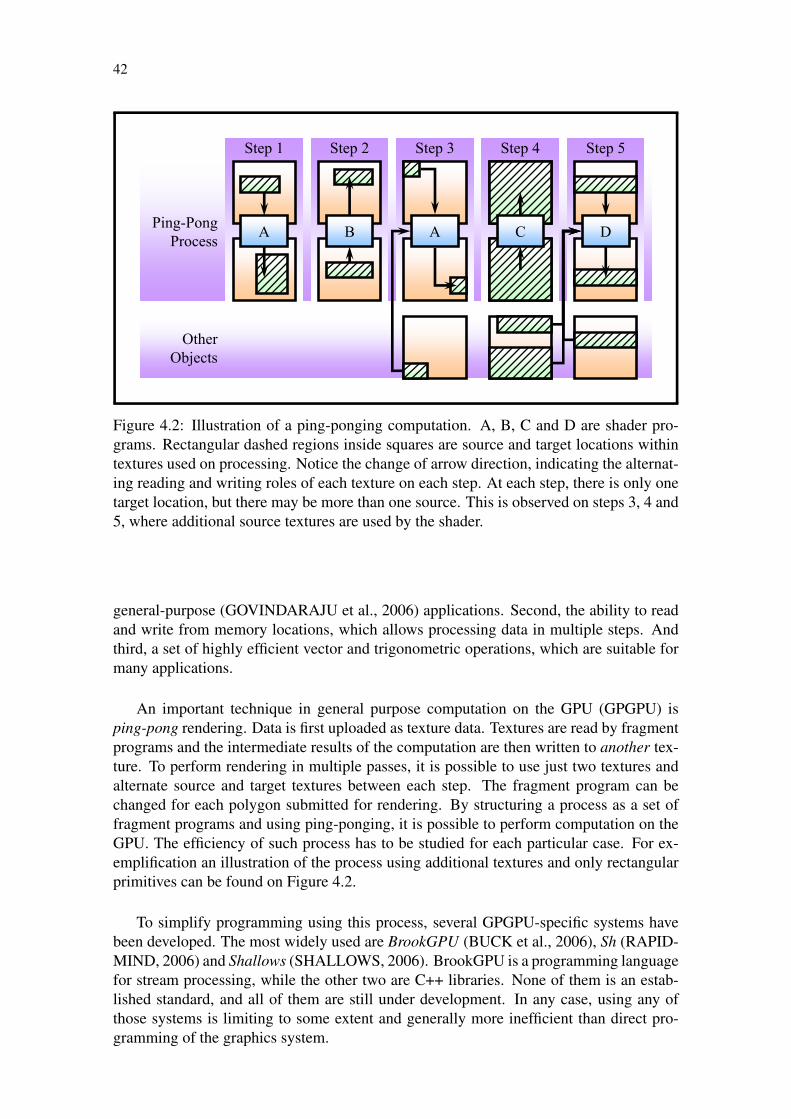
42

OtherObjects

Step 1

Ping-PongProcess

Step 2 Step 3 Step 4 Step 5

AB CA D

Figure 4.2: Illustration of a ping-ponging computation. A, B, C and D are shader pro-grams. Rectangular dashed regions inside squares are source and target locations withintextures used on processing. Notice the change of arrow direction, indicating the alternat-ing reading and writing roles of each texture on each step. At each step, there is only onetarget location, but there may be more than one source. This is observed on steps 3, 4 and5, where additional source textures are used by the shader.

general-purpose (GOVINDARAJU et al., 2006) applications. Second, the ability to readand write from memory locations, which allows processing data in multiple steps. Andthird, a set of highly efficient vector and trigonometric operations, which are suitable formany applications.

An important technique in general purpose computation on the GPU (GPGPU) isping-pong rendering. Data is first uploaded as texture data. Textures are read by fragmentprograms and the intermediate results of the computation are then written to another tex-ture. To perform rendering in multiple passes, it is possible to use just two textures andalternate source and target textures between each step. The fragment program can bechanged for each polygon submitted for rendering. By structuring a process as a set offragment programs and using ping-ponging, it is possible to perform computation on theGPU. The efficiency of such process has to be studied for each particular case. For ex-emplification an illustration of the process using additional textures and only rectangularprimitives can be found on Figure 4.2.

To simplify programming using this process, several GPGPU-specific systems havebeen developed. The most widely used are BrookGPU (BUCK et al., 2006), Sh (RAPID-MIND, 2006) and Shallows (SHALLOWS, 2006). BrookGPU is a programming languagefor stream processing, while the other two are C++ libraries. None of them is an estab-lished standard, and all of them are still under development. In any case, using any ofthose systems is limiting to some extent and generally more inefficient than direct pro-gramming of the graphics system.

43

Table 4.1: Mapping audio concepts to graphic concepts.Audio Concept Graphics Concept

Sample FragmentAmplitude Color (Luminance)Processor Shader

Computation ShadingBlock Texture Row

Pointers Texture Coordinates

4.2 Using the GPU for Audio Processing

Before using the GPU, one needs to define a mapping between audio and graphicsconcepts. This is given explicitly on Table 4.1 and illustrated on Figure 4.3. First, texelsand samples are just memory variables containing values, so samples can be transformedinto texels. Second, a texel is built of several color components (for instance, red, green,blue and transparency levels), which actually makes a texel a small sequence of values;similarly, audio is encoded in channels, and one common representation of audio is bycyclically interleaving one sample from each channel on each position of an array. There-fore, a group of samples referring to the same instant and different audio channels canbe trivially mapped into the color components of a single texel. In an audio application,blocks of n samples are processed in each step. Treating a texture as a bidimensionalmatrix, the contents of blocks can be stored in many different ways. One could see a bidi-mensional matrix as an array of same-sized arrays, which can be either lines or columnsof the matrix. Then, an audio block can be mapped into one of these arrays, and, at eachstep, the CPU can issue the drawing of a line primitive providing the coordinates of theleftmost and rightmost texels of the line where the block was stored. Processing of theblock, then, is performed by the fragment shader. From the rasterization stage, fragmentsare generated for each texel holding a sample. The parameters specified for the line prim-itive’s vertices are interpolated according to the position of the fragment in the line andare used in the computation of the output color (a new sample value), which is stored inthe corresponding position on another texture. The graphics hardware can be instructedto change the textures it reads and writes from at each step, so that other shaders can runtaking as input the output of a preceding step. At last, when processing a single audioblock, the computation may require many steps on the GPU.

Specifying vertices of a primitive can be viewed as posting a task for computationon the GPU. In the case of this work, tasks are always horizontal lines or, eventually,quadrilaterals, if more than 4 channels are needed—then, a single signal block takes morethan a single line, and each line (except for the last one) holds 4 blocks of audio, one foreach audio channel.

GPUs are able to perform many arithmetic operations that are useful when processingaudio. Besides addition and multiplication, shading languages provide operations suchas linear interpolation (which may be used for resampling or to interpolate variable in-put parameters), trigonometric functions (which are often used for synthesis), clamping(which may be a post-processing in cases where the sound card requires values withina specific range), step functions (which could be used to implement stepwise functions,such as envelopes), swizzling (which could be used to route signals between channels)and a random functions (which can be used to implement noise).

44

Texture AudioSamples

0 1 ...01

...

y

x x0 1 ...Texels

RGBA

Color

Samples

Channels

Channels

(a) The mapping between a block of 4 samples and a line of texels at vertical position y. The samples atposition x in the block are mapped into coordinate 〈x, y〉 in the texture. Audio channels (1, 2, 3, 4) aremapped into color components (R, G, B, A, respectively).

SourceTexture

TargetTexture

ShaderProgram

a b

(b) Application of a shader to one block at position a on the source texture, producing a new block of samplesat position b on the target texture. In this case, the fragment processor has 4 individual pipelines (solid lines),so 4 samples, each with 4 channels, are processed simultaneously.

1 2 3 4 5

...

(c) A representation of ping-ponging using shaders 1, 2, 3, 4 and 5, in this order. Notice that the results ofone step are used in the subsequent step.

Figure 4.3: Full illustration of audio processing on the GPU.

45

Before using the graphics hardware for effective computation of audio, the OpenGLstate must be defined. For more information on this, see Appendix C.

Remark The reason for using the ping-pong technique is that hardware implementationof texture access considers them read-only or write-only but not read-write. We cannotset a texture as source and target at the same time because doing this will produce raceconditions in most cases. GPUs implement separate read and write caches, and writing toa texture does not cause the read caches to be updated.

At this point, we have several tools to process signals on the GPU already. To rendera sinusoidal wave, for example, one would write a shader to evaluate the sinusoidal wave,load it, set the target texture, post a line as suggested in Figure 4.3, and then read theresults back to the main memory. Clearly, this data can be then passed to the audiocallback procedure for playing. Therefore, the next section describes how a modulararchitecture can be implemented based on the GPU and how control information can bemanaged on a modular system.

4.3 Module System

Recall from Section 3.2.2.1 that an useful way to program audio systems is by defininga processing model graphically, interconnecting inputs and outputs of modules. Besidesinputs and outputs, modules also have parameters that define their actual effect on theinput data, and they also receive events, which are used to trigger the generation of notesand to change the module parameters.

Each module may have fixed or variable polyphony. In the second case, a list of play-ing notes can be created to represent a set of notes being played together. Every time acertain event occurs (e.g., a MIDI “note on” or a keyboard “key down”), an instance ofan object representing the internal state of the note is added to this list. The implemen-tation of such object varies according to the needs of the module. For example, a simpledrum machine needs only a pointer to a percussion instrument. A wavetable synthesizer,though, needs the pitch and a pointer to a wavetable. Generally, since notes may extendfor more than one block, one needs to represent the elapsed time since the note started toplay. Thus, elapsed time is normally a member of a note’s internal state.

In our implementation, we actually replace time by a phase offset. Assuming thatperiodic waveforms have a period of T and given the periodicity of the primitive wavesand of those obtained by wavetable synthesis, the time parameter can be mapped into therange [0, 1) −kT , resulting in a value into the range [0, 1). This value is called the phaseoffset.

In our implementation, event processing is performed at the block generation cycleinside the producer thread. How a module behaves when it receives a control event isimplementation-dependent: one may prefer, for example, to implement smooth changesof a module’s parameters to ensure that the wave is kept smooth along time.

The next step is to post the necessary geometric primitives to achieve the desiredprocessing on the GPU. The order of operations is also customizable. One could devisean algorithm to position blocks of audio generated by each module in the textures alongthe steps of ping-ponging1.

1 See Section 6.1.

46

Listing 4.1: Sinusoidal wave shader.1 f loa t4 main (2 f loa t2 Params : TEXCOORD0) : COLOR3 {4 f l o a t t = Params . x ;5 f l o a t a = Params . y ;6 f l o a t w = a∗ (0 .5∗ s in (6.28318530717958∗ t ) ) ;7 return f loa t4 (w, w, w, w ) ;8 } ;

Listing 4.2: Sinusoidal wave generator using the CPU.1 void SinusoidalWave (2 f l o a t nPhase1 , f l o a t nPhase2 ,3 f l o a t ∗pBuf fer , long nSamples )4 {5 f l o a t nPhaseStart = 2.0 ∗ M_PI ∗ nPhase1 ;6 f l o a t nRate = 2.0 ∗ M_PI ∗ ( nPhase2 − nPhase1 ) / nSamples ;7 for ( i n t i = 0 ; i < nSamples ; i ++)8 {9 f l o a t u = nPhaseStart + nIndex ∗ nRate ;

10 pBuf fe r [ i ] = s in ( u ) ;11 }12 }

4.4 Implementation

Our application was written in the C++ language using OpenGL and Cg for graphicsprocessing and RtAudio for audio streaming. Source code was compiled with optimiza-tions using Microsoft Visual Studio .NET 2003 (MICROSOFT, 2006b).

The following sections present the implementation of several audio processing tasksusing shaders. We have written the shaders to point out clearly how the formulas wepresented are applied.

4.4.1 Primitive Waveforms

Rendering primitive waveforms consists of evaluating an equation, given the param-eter to the formula. Listing 4.1, Listing 4.3, Listing 4.4 and Listing 4.5 implement therendering of primitive waveforms according to the equations presented on Table 3.2, andListing 4.2 shows how a sinusoidal wave can be rendered using the CPU. The shadersinclude an amplitude parameter that is used to perform envelope shaping.

4.4.2 Mixing

A mixing shader consists simply of summing selected lines in textures. The positionof these lines is determined by the module. When a signal has more than 4 channels, itis represented as a set of consecutive lines, each holding up to 4 channels. Therefore, themixing shader needs to support this format and sum corresponding channels. Figure 4.4illustrates this, and Listing 4.6 presents the implementation of the shader.

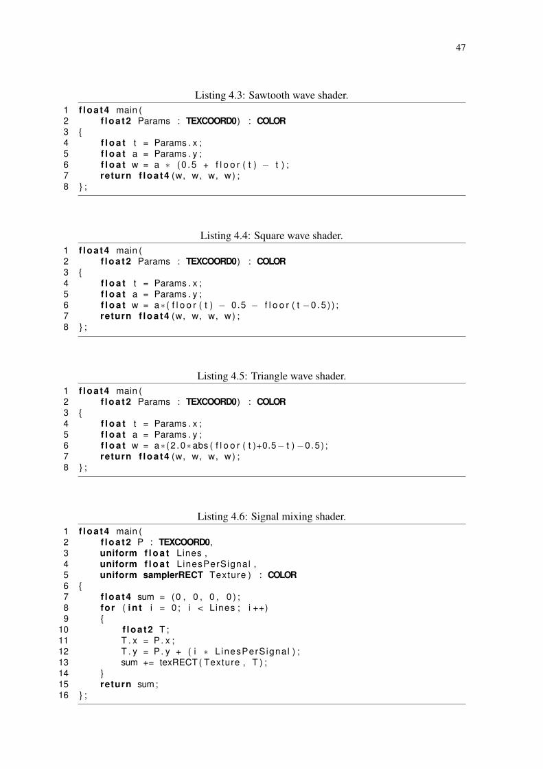
47

Listing 4.3: Sawtooth wave shader.1 f loa t4 main (2 f loa t2 Params : TEXCOORD0) : COLOR3 {4 f l o a t t = Params . x ;5 f l o a t a = Params . y ;6 f l o a t w = a ∗ ( 0 .5 + f l o o r ( t ) − t ) ;7 return f loa t4 (w, w, w, w ) ;8 } ;

Listing 4.4: Square wave shader.1 f loa t4 main (2 f loa t2 Params : TEXCOORD0) : COLOR3 {4 f l o a t t = Params . x ;5 f l o a t a = Params . y ;6 f l o a t w = a∗ ( f l o o r ( t ) − 0.5 − f l o o r ( t −0 .5 ) ) ;7 return f loa t4 (w, w, w, w ) ;8 } ;

Listing 4.5: Triangle wave shader.1 f loa t4 main (2 f loa t2 Params : TEXCOORD0) : COLOR3 {4 f l o a t t = Params . x ;5 f l o a t a = Params . y ;6 f l o a t w = a∗ (2 .0∗ abs ( f l o o r ( t )+0.5− t ) −0.5) ;7 return f loa t4 (w, w, w, w ) ;8 } ;

Listing 4.6: Signal mixing shader.1 f loa t4 main (2 f loa t2 P : TEXCOORD0,3 uniform f l o a t Lines ,4 uniform f l o a t LinesPerSignal ,5 uniform samplerRECT Texture ) : COLOR6 {7 f loa t4 sum = (0 , 0 , 0 , 0 ) ;8 for ( i n t i = 0 ; i < Lines ; i ++)9 {

10 f loa t2 T ;11 T . x = P. x ;12 T . y = P. y + ( i ∗ LinesPerSignal ) ;13 sum += texRECT ( Texture , T ) ;14 }15 return sum;16 } ;

48

Texture A Texture B

Channels 1–4Channels 5–8Channels 9

Channels 1–4Channels 5–8

Channel 9

Channels 1–4Channels 5–8

Channel 9

Channels 1–4Channels 5–8

Channel 9∑

Figure 4.4: Illustration of usage of mixing shaders with 10-channel signals. Each smallerrectangle represents a line in the respective texture.

4.4.3 Wavetable Resampling

Our implementation of wavetable resampling extends the definition given on Sec-tion 3.2.3.3 by supporting a crossfade between two wavetables. Crossfading consists offading from one into another. In this case, that means reducing gradually the amplitudeof one wave while the amplitude of the other one is increased. The shader receives thename of the two textures holding the tables, the size of those textures, and an interpolatedvalue for the amplitude and for the crossfading. Listing 4.7 presents the source code forthe shader. Listing 4.8 shows the parameters assigned to vertices when the line is postedfor rendering. Listing 4.9 presents an abstract algorithm for managing a note’s state usingan ADSR envelope and the wavetable shader. In this case, 5 wave tables are used andcrossfaded in each of the A, D, S and R steps.

4.4.4 Echo Effect

As discussed on Section 3.2.3.4, an echo effect requires the value of the current inputsample and a past output sample, offset by k samples from the current sample. This valuemust be accessible, so a set of past input blocks must be saved using some mechanism.For that, we can create an extra texture with the same dimensions as those of the primarytextures used for ping-ponging. On that texture, blocks are stored and updated as in acircular buffer: when the pointer to the back of the buffer reaches the highest possibleindex, it is wrapped down to the first index instead of being incremented. Usually, echoespresent more than 100 ms of delay, so we can restrict an echo’s delay time to the timeduration of the block size. The value of input and output samples are both scaled byconstants. To simplify this operation, we create an useful shader to perform additionand multiplication by a constant in a single step: the MADD shader (Listing 4.11 andListing 4.12). At last, a copy shader (Listing 4.10) is required because we cannot readand write from the extra texture at the same time. The operation of the echo module usingMADD shaders and the copy shader is given textually on Listing 4.13 and is illustratedon Figure 4.5.

49

Listing 4.7: Wavetable shader with crossfading between two tables.1 f loa t4 main (2 f loa t4 Params : TEXCOORD0,3 uniform f loa t2 S,4 uniform samplerRECT Texture1 ,5 uniform samplerRECT Texture2 ) : COLOR6 {7 / / Table o f f s e t s8 f l o a t o1 = Params . x ;9 f l o a t o2 = Params . y ;

1011 / / I n t e r p o l a t o r s12 f l o a t i = Params . z ;13 f l o a t a = Params .w;1415 / / L inear sampling16 f l o a t s11 = texRECT ( Texture1 ,17 f loa t2 ( f l o o r ( fmod ( o1 , S . x ) ) , 0 . 0 ) ) ;18 f l o a t s12 = texRECT ( Texture1 ,19 f loa t2 ( f l o o r ( fmod ( o1+1 , S . x ) ) , 0 . 0 ) ) ;20 f l o a t s1 = l e r p ( s11 , s12 , f r a c ( o1 ) ) ;21 f l o a t s21 = texRECT ( Texture2 ,22 f loa t2 ( f l o o r ( fmod ( o2 , S . y ) ) , 0 . 0 ) ) ;23 f l o a t s22 = texRECT ( Texture2 ,24 f loa t2 ( f l o o r ( fmod ( o2+1 , S . y ) ) , 0 . 0 ) ) ;25 f l o a t s2 = l e r p ( s21 , s22 , f r a c ( o2 ) ) ;2627 / / Mix ing28 f l o a t w = a ∗ l e r p ( s1 , s2 , i ) ;29 return f loa t4 (w, w, w, w ) ;30 } ;

Listing 4.8: Primitive posting for the wavetable shader.1 cgGLSetTextureParameter ( ParamTexture1 , Texture1 ) ;2 cgGLSetTextureParameter ( ParamTexture2 , Texture2 ) ;3 cgGLEnableTextureParameter ( ParamTexture1 ) ;4 cgGLEnableTextureParameter ( ParamTexture2 ) ;5 cgGLSetParameter2f (ParamS , Texture1_Size , Texture2_Size ) ;67 glBegin (GL_LINES ) ;8 g lMul t iTexCoord4f (GL_TEXTURE0,9 O f f s e t _ S t a r t ∗ Texture1_Size , O f f s e t _ S t a r t ∗ Texture2_Size ,

10 I n t e r p o l a t o r _ S t a r t , Ampl i tude_Star t ) ;11 g l V e r t e x 2 i ( First_Sample , Target_Row ) ;12 g lMul t iTexCoord4f (GL_TEXTURE0,13 Offset_End ∗ Texture1_Size , Offset_End ∗ Texture2_Size ,14 In te rpo la to r_End , Amplitude_End ) ;15 g l V e r t e x 2 i ( Last_Sample , Target_Row ) ;16 glEnd ( ) ;

50

Listing 4.9: Note state update and primitive posting.1 do2 c a l c u l a t e t ime to next stage change3 i f stage i s e i t h e r A, D or R4 i f next stage change occurs i n cu r ren t b lock5 update s ta te v a r i a b l e s to next stage change6 else7 update s ta te v a r i a b l e s to cu r ren t b l o c k ’ s end8 else9 update s ta te v a r i a b l e s to cu r ren t b l o c k ’ s end

1011 evaluate ampl i tude and i n t e r p o l a t o r values12 evaluate cu r ren t phase1314 post l i n e p r i m i t i v e using the wavetable shader15 {16 set o1 and o2 to the cu r ren t sample o f f s e t s w i t h i n each tab le17 set i to the i n t e r p o l a t o r value18 set a to the ampl i tude value19 set Texture1 and Texture2 to cu r ren t s tage ’s wavetables20 }21 update stage c o n t r o l va r i a b l e s22 repeat u n t i l a l l b lock i s processed

Listing 4.10: Copy shader.1 f loa t4 main (2 f loa t2 P : TEXCOORD0,3 uniform samplerRECT Texture ) : COLOR4 {5 return texRECT ( Texture , P ) ;6 } ;

Listing 4.11: Multiply and add shader.1 f loa t4 main (2 f loa t2 Pos i t ionX : TEXCOORD0,3 f loa t2 Pos i t ionY : TEXCOORD1,4 uniform f l o a t Alpha ,5 uniform samplerRECT TextureX ,6 uniform samplerRECT TextureY ) : COLOR7 {8 f loa t4 X = texRECT ( TextureX , Pos i t ionX ) ;9 f loa t4 Y = texRECT ( TextureY , Pos i t ionY ) ;

10 return Alpha ∗ X + Y;11 } ;

51

Listing 4.12: Primitive posting for the multiply and add shader.1 cgGLSetParameter1f ( ParamAlpha , Alpha ) ;2 cgGLSetTextureParameter ( ParamTextureX , TextureX ) ;3 cgGLSetTextureParameter ( ParamTextureY , TextureY ) ;4 cgGLEnableTextureParameter ( ParamTextureX ) ;5 cgGLEnableTextureParameter ( ParamTextureY ) ;67 glBegin (GL_LINES ) ;8 g lMul t iTexCoord2 i (GL_TEXTURE0, 0 , Row_in_TextureX ) ;9 g lMul t iTexCoord2 i (GL_TEXTURE1, 0 , Row_in_TextureY ) ;

10 g l V e r t e x 2 i (0 , Draw_Row ) ;11 g lMul t iTexCoord2 i (GL_TEXTURE0, n , Row_in_TextureX ) ;12 g lMul t iTexCoord2 i (GL_TEXTURE1, n , Row_in_TextureY ) ;13 g l V e r t e x 2 i ( n , Draw_Row ) ;14 glEnd ( ) ;

Listing 4.13: Echo processor shader call sequence.1 post l i n e p r i m i t i v e using the m u l t i p l y and add shader2 {3 set a to feedback gain value4 set TextureX to Texture 45 set Pos i t ionX to the delay l i n e ’ s read p o s i t i o n6 set TextureY to Texture 17 set Pos i t ionY to row 08 render to Texture 39 }

10 post l i n e p r i m i t i v e using the m u l t i p l y and add shader11 {12 set a to wet mix gain value13 set TextureX to Texture 414 set Pos i t ionX to the delay l i n e ’ s read p o s i t i o n15 set TextureY to Texture 116 set Pos i t ionY to row 017 render to Texture 218 }19 copy generated block from t e x t u r e 3 to t e x t u r e 4 at the delay l i n e ’ s w r i t e p o s i t i o n20 update delay l i n e read and w r i t e p o s i t i o n s

52

Step 2

Step 3

Step 1 FrontBackMADD Shader

FrontBackMADD Shader

FrontBack

Copy Shader

Texture 1 Texture 2 Texture 3 Texture 4

Figure 4.5: Illustration of steps to compute an echo effect on the GPU using MADDshaders and one copy operation. Notice that texture 3 is used to store a temporary resultthat ends up copied into texture 4 at the “front” position of a circular buffer. The actualoutput of the module is written on texture 2.

4.4.5 Filters

The implementation of a FIR filter follows the same idea of the past shaders: directlytranslate the formula into a shader and use it by rendering a line primitive. For filters, sev-eral samples of the past input block will be necessary; they can be saved on the auxiliarytexture following the idea presented for the echo effect.

An IIR filter presents an implementation problem: it requires the value of outputsamples that are being generated in the same step. As a result, the part of Equation (3.8)using output values cannot be implemented trivially. IIR filters are still implementable,but the speed up obtained by a GPU implementation will not be as significant as theremaining shaders. For this reason, we have not implemented IIR filters.

4.5 Summary

This chapter described the structure of an audio application. We discussed how audiois passed on to the audio device and the reasons to implement an intermediary bufferbetween the application and the audio interface. We presented details about graphicsrendering and how graphics APIs such as OpenGL can be used to instruct the GPU abouthow to process audio data. At last, we discussed the implementation of modular systemsand presented shaders to perform audio processing on the graphics device.

In the following chapter, the performance of this system is measured. We discussthe quality of the generated signal and the limitations imposed by the GPU for audioprocessing.

53

5 RESULTS

In this chapter, we discuss the results obtained with the implementation described onthe last chapter. In the first section, we present a comparison of total polyphony achievedwith both a CPU and a GPU version of algorithms for primitive waveform generation. Thenext section evaluates the quality of audio data produced by the GPU. Then, we presentthe limitations posed by the graphics hardware on audio processing.

5.1 Performance Measurements

The following measurements were obtained by running the application on an AMDAthlon64 3000+ (1.81 GHz) with 1 GB of memory with an ASUS A8N-SLI Deluxemotherboard, a PCI Express nVidia GeForce 6600 with 256 MB, and a Cretive AudigyPlatinum eX sound card. These devices allowed a texture size of 4096 texels in eachdimension and audio blocks of 96 to 2400 samples. Although we have used a 64-bitprocessor, we were running the application on Windows XP, which does not support 64-bit instructions and, therefore, the system was running in 32-bit emulation mode.

We used blocks of 256 samples and set the ASIO audio device to play at a samplingrate of 48 kHz using 2 channels. At this rate, 256 samples represents a little more than5 ms. The intermediary buffer between the callback and the producer thread was able tohold 2 blocks. Holding the block on the buffer causes a total delay of about 11 ms, whichis acceptable for real-time output.

To compare the performance of the GPU with similar CPU implementations, we ren-dered the basic waveforms many times on subsequent rows of a texture. We wrote similarrendering algorithms on the CPU. For example, we present the sine wave generator onListing 4.2 with code that runs on the CPU. Implementations for other shaders have beendeveloped similarly. One may argue that there are more efficient implementations of asine wave oscillator, but we note that other methods have drawbacks (sometimes accept-able), such as introducing noise (by sampling a wavetable) or becoming innacurate alongtime (by using only addition and multiplication to resolve a differential equation). Addi-tionally, the implementation by directly evaluating a formula constitutes a more preciseoverall performance comparison, since both machines would be performing essentiallythe same computation.

We approximated the maximum number of times the rendering programs for the GPUand CPU could be invoked in real time without causing audio glitches. To do that, wegradually increased the number of line primitives being posted and programmed the codein the callback to update a counter whenever no block was present for output. By doingthis rather than simply calculating the time that the GPU takes to process a certain amountof lines, one gets results that express how the application behaves on practical usage by

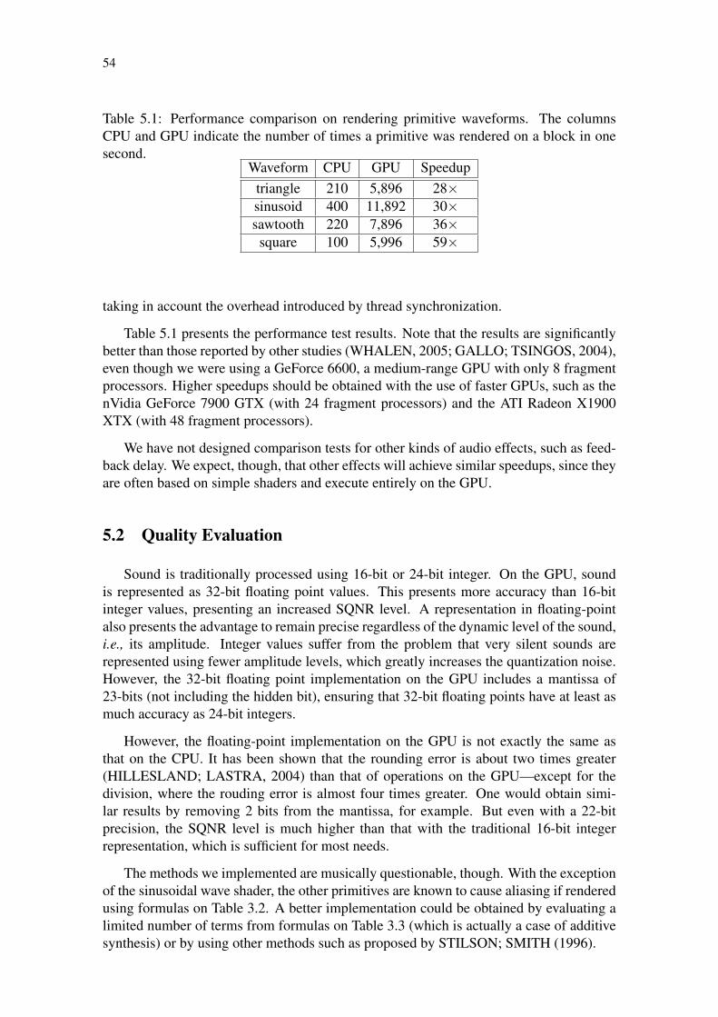
54

Table 5.1: Performance comparison on rendering primitive waveforms. The columnsCPU and GPU indicate the number of times a primitive was rendered on a block in onesecond.

Waveform CPU GPU Speeduptriangle 210 5,896 28×sinusoid 400 11,892 30×sawtooth 220 7,896 36×square 100 5,996 59×

taking in account the overhead introduced by thread synchronization.

Table 5.1 presents the performance test results. Note that the results are significantlybetter than those reported by other studies (WHALEN, 2005; GALLO; TSINGOS, 2004),even though we were using a GeForce 6600, a medium-range GPU with only 8 fragmentprocessors. Higher speedups should be obtained with the use of faster GPUs, such as thenVidia GeForce 7900 GTX (with 24 fragment processors) and the ATI Radeon X1900XTX (with 48 fragment processors).

We have not designed comparison tests for other kinds of audio effects, such as feed-back delay. We expect, though, that other effects will achieve similar speedups, since theyare often based on simple shaders and execute entirely on the GPU.

5.2 Quality Evaluation

Sound is traditionally processed using 16-bit or 24-bit integer. On the GPU, soundis represented as 32-bit floating point values. This presents more accuracy than 16-bitinteger values, presenting an increased SQNR level. A representation in floating-pointalso presents the advantage to remain precise regardless of the dynamic level of the sound,i.e., its amplitude. Integer values suffer from the problem that very silent sounds arerepresented using fewer amplitude levels, which greatly increases the quantization noise.However, the 32-bit floating point implementation on the GPU includes a mantissa of23-bits (not including the hidden bit), ensuring that 32-bit floating points have at least asmuch accuracy as 24-bit integers.

However, the floating-point implementation on the GPU is not exactly the same asthat on the CPU. It has been shown that the rounding error is about two times greater(HILLESLAND; LASTRA, 2004) than that of operations on the GPU—except for thedivision, where the rouding error is almost four times greater. One would obtain simi-lar results by removing 2 bits from the mantissa, for example. But even with a 22-bitprecision, the SQNR level is much higher than that with the traditional 16-bit integerrepresentation, which is sufficient for most needs.

The methods we implemented are musically questionable, though. With the exceptionof the sinusoidal wave shader, the other primitives are known to cause aliasing if renderedusing formulas on Table 3.2. A better implementation could be obtained by evaluating alimited number of terms from formulas on Table 3.3 (which is actually a case of additivesynthesis) or by using other methods such as proposed by STILSON; SMITH (1996).

55

5.3 Limitations

Several processes that do not present local data independence do not map well to theGPU. In our work, the most prominent example of that is the IIR filter. To implementan IIR filter efficiently, one would need to access the values computed for fragments tothe left of the current fragment. Given that a texture cannot be read and written in thesame step, this would require evaluating fragment by fragment and exchanging sourceand target textures between the evaluation of every fragment. Naturally, this represents abottleneck, since one needs to submit many geometric primitives and force cache updatesfor each fragment. Even with the latest GPUs, the CPU implementation should probablypresent better performance. This problem is still under study, but it seems there are at leasta few special cases for which a performance gain can be achieved. Note that this problemwould be solved if the ability to access the values computed for adjacent fragments in asingle step were available at the graphics hardware.

5.4 Summary

This chapter presented the results we obtained by inspecting the application. We haveshown that a GPU-based implementation of several algorithms may present a speedup of59×. We have explained that the quality of signals generated on the GPU is adequateand very closely related to professional 24-bit quality, except that the usage of floating-point introduces less quantization error on low-amplitude samples. The problem of datadependency, which directly affects the implementation of IIR filters, was also discussed.

56

6 FINAL REMARKS

This work has presented the implementation of an audio processing system usingthe GPU that produces results in real-time, achieves higher performance and is easilyextensible. The fundamental concepts of sound processing were presented, prior to adiscussion of the structure of an audio processing system and the implication of everydesign choice. We have presented how to use fragment shaders to perform computationof audio samples, and we also designed performance benchmarks for comparison anddiscussed the current limitations of the system. This work ultimately demonstrates thatthe GPU can be used for efficient audio processing, achieving speedups of almost 60×in some cases, enabling users to take advantage of more computational power with theflexibility of software implementations at costs lower than professional audio equipments.

6.1 Future Work

This system is a prototype including several modules for demonstration. For profes-sional music, many other modules need to be implemented, including an IIR filter, which,as discussed, could not be mapped efficiently using a direct approach.

We also presented the concept of modular processing, yet we have not developed acomplete module system that would allow user customization of a processing model. Toachieve this, one needs to implement an auxiliary system to distribute the usage of texturelines in each step of ping-ponging to each of the modules, as necessary according tothe processing model. This is a required abstraction for efficient development, since theactual implementation of a module does not depend on which line of a texture it is readingfrom, but requires that this line matches the line where the results of another module werewritten. This auxiliary system would also be required to insert implicit operations, such asmixing two output signals that are connected to the input of a module before performingthat module’s computation. We have planned an algorithm to do that, but we do notpresent it here due to lack of time for testing.

An interesting addition would be Sony DSD, a recent sound format commonly used inprocessing high quality audio. This format uses delta-sigma modulation to represent thesignal, and there are algorithms for several audio processes already (REISS; SANDLER,2004). Whether this format can be efficiently processed by the GPU is the most importantquestion. If it can, implementing DSD support could be useful, since the amount of datato be processed is relatively close to that necessary to process PCM audio1. Another

1 A common DSD format is 1-bit samples at 2822,4 kHz (64 ∗ 44.1 kHz), which results in approximately 2to 4 times as much as the usual CD PCM format. A proposed alternative format would be to represent each1 bit sample by 1 byte words, taking 64 times more storage space. Advantages of each alternative remainto be studied.

57

interesting addition would be the support to time-varying frequency-domain signals, inorder to evaluate the efficiency of the GPU for this kind of computation. This wouldintroduce more implicit operations to be handled.

A commercial solution would also require the addition of a graphics interface, a se-quencer and the inclusion of sample banks that can be used by the musician to createmusic.

58

REFERENCES

ANSARI, M. Y. Video Image Processing Using Shaders. Game Developers Conference,Presentation.

DIRECTOR, S. W. (Ed.). Digital Filters: analysis and design. TMH ed. New Delhi,India: Tata McGraw-Hill, 1980.

AUDIO DSP TEAM. Resampling. Available at: <http://www.dspteam.com/resample.html>. Visited in: June 2006.

BIONICFX. 2005. Available at: <http://www.bionicfx.com>. Visited in: June 2006.

BRISTOW-JOHNSON, R. Wavetable Synthesis 101, A Fundamental Perspective. In:AES CONVENTION, 101., 1996, Los Angeles, California. Proceedings. . . [S.l.: s.n.],1996. Available at: <http://www.musicdsp.org/files/Wavetable-101.pdf>.

BUCK, I.; FOLEY, T.; HORN, D.; SUGERMAN, J.; FATAHALIAN, K.; HOUSTON,M.; HANRAHAN, P. Brook for GPUs: stream computing on graphics hardware. ACMTransactions on Graphics, [S.l.], v.23, n.3, p.777–786, August 2004. Available at: <http://graphics.stanford.edu/papers/brookgpu/brookgpu.pdf>. Visited in: June 2006.

BUCK, I.; FOLEY, T.; HORN, D.; SUGERMAN, J.; HANRAHAN, P.; HOUSTON,M.; FATAHALIAN, K. BrookGPU. 2006. Available at: <http://graphics.stanford.edu/projects/brookgpu>. Visited in: June 2006.

GALLO, E.; TSINGOS, N. Efficient 3D Audio Processing with the GPU. Proceedingsof GP2: Workshop on General Purpose Computing on Graphics Processors, LosAngeles, California, August 2004. Poster. Available at: <http://www-sop.inria.fr/reves/Nicolas.Tsingos/publis/posterfinal.pdf>. Visited in: June 2006.

GOVINDARAJU, N. K.; GRAY, J.; KUMAR, R.; MANOCHA, D. GPUTeraSort: highperformance graphics coprocessor sorting for large database management. In: ACMSIGMOD INTERNATIONAL CONFERENCE ON MANAGEMENT OF DATA, 2003.,2006, Chicago, IL. Proceedings. . . [S.l.: s.n.], 2006. Available at: <http://gamma.cs.unc.edu/GPUTERASORT/gputerasort_sigmod06.pdf>.

GPUFFTW Library. Sponsored by Army Modeling and Simulation Office, Army Re-search Office, Defense Advanced Research Projects Agency, RDECOM and NVIDIACorporation. Available at: <http://gamma.cs.unc.edu/GPUFFTW>.

GUMMER, A. W. (Ed.). Biophysics of the Cochlea. Titisee, Germany: [s.n.], 2002.Proceedings of the International Symposium.

59

OPPENHEIM, A. V. (Ed.). Digital Filters. 3rd ed. Englewood Cliffs, NJ, USA: Prentice-Hall, 1989. (Signal Processing Series).

HILLESLAND, K. E.; LASTRA, A. GPU Floating-Point Paranoia. In: GP2: WORK-SHOP ON GENERAL PURPOSE COMPUTING ON GRAPHICS PROCESSORS,2004, Chapel Hill, NC, USA. Proceedings. . . ACM SIGGRAPH, 2004. Available at:<http://www.cs.unc.edu/~ibr/projects/paranoia/gpu_paranoia.pdf>. Visited in: June 2006.

ISHIKAWA, O.; AONO, Y.; KATAYOSE, H.; INOKUCHI, S. Extraction of Musical Per-formance Rules Using a Modified Algorithm of Multiple Regression Analysis. In: IN-TERNATIONAL COMPUTER MUSIC CONFERENCE, 2000, Berlin, Germany, August2000. Proceedings. . . [S.l.: s.n.], 2000. p.348–351. Available at: <http://www-inolab.sys.es.osaka-u.ac.jp/users/ishikawa/kenkyu/study/ICMC2000.pdf>. Visited in: June 2006.

JEDRZEJEWSKI, M.; MARASEK, K. Computation of Room Acoustics Using Pro-grammable Video Hardware. In: INTERNATIONAL CONFERENCE ON COMPUTERVISION AND GRAPHICS, 2004, Warsaw, Poland. Anais. . . [S.l.: s.n.], 2004. Availableat: <http://www.pjwstk.edu.pl/~s1525/prg/mgr/gpuarticle.pdf>. Visited in: June 2006.

JULIANO, J.; SANDMEL, J.; AKELEY, K.; ALLEN, J.; BERETTA, B.; BROWN,P.; CRAIGHEAD, M.; EDDY, A.; EVERITT, C.; GALVAN, M.; GOLD, M.; HART,E.; KILGARD, M.; KIRKLAND, D.; LEECH, J.; LICEA-KANE, B.; LICHTENBELT,B.; LIN, K.; MACE, R.; MORRISON, T.; NIEDERAUER, C.; PAUL, B.; PUEY,P.; ROMANICK, I.; ROSASCO, J.; SAMS, R. J.; SEGAL, M.; SEETHARAMAIAH,A.; SCHAMEL, F.; VOGEL, D.; WERNESS, E.; WOOLLEY, C. Framebuffer Ob-ject. Revision 118. Available at: <http://oss.sgi.com/projects/ogl-sample/registry/EXT/framebuffer_object.txt>. Visited in: June 2006.

KESSENICH, J.; BALDWIN, D.; ROST, R. The OpenGL Shading Language. 1.10,Revision 59 ed. Madison, AL, USA: 3Dlabs, Inc. Ltd., 2004. Available at: <http://oss.sgi.com/projects/ogl-sample/registry/ARB/GLSLangSpec.Full.1.10.59.pdf>. Visited in:June 2006.

KURO5HIN. The End of Moore’s Law. Available at: <http://www.kuro5hin.org/story/2005/4/19/202244/053>. Visited in: June 2006.

MICROSOFT CORPORATION. HLSL Shaders. 2005. Available at: <http://msdn.microsoft.com/library/en-us/directx9_c/Writing_HLSL_Shaders.asp>. Visited in: June2006.

MICROSOFT CORPORATION. DirectSound C/C++ Reference. Available at: <http://msdn.microsoft.com/library/en-us/directx9_c/dx9_directsound_reference.asp>. Visitedin: June 2006.

MICROSOFT CORPORATION. Visual Studio .NET 2003. Available at: <http://msdn.microsoft.com/vstudio/previous/2003>. Visited in: May 2006.

ROTTINO, M. P. (Ed.). Elements of Computer Music. Upper Saddle River, NJ, USA:PTR Prentice Hall, 1990.

MOORE, G. E. Cramming More Components onto Integrated Circuits. Electronics,[S.l.], v.38, n.8, p.114–117, April 1965. Available at: <ftp://download.intel.com/research/silicon/moorespaper.pdf>.

60

MORELAND, K.; ANGEL, E. The FFT on a GPU. In: SIGGRAPH/EUROGRAPH-ICS WORKSHOP ON GRAPHICS HARDWARE, 2003, San Diego, CA. Anais. . . Eu-rographics Association, 2003. p.112–119. Available at: <http://www.eg.org/EG/DL/WS/EGGH03/112-119-moreland.pdf>. Visited in: June 2006.

NVIDIA CORPORATION. Cg Toolkit User’s Manual. 1.4.1 ed. Santa Clara, CA, USA:NVIDIA Corporation, 2006. Available at: <http://download.nvidia.com/developer/cg/Cg_1.4/1.4.1/Cg-1.4.1_UsersManual.pdf>. Visited in: June 2006.

POLICARPO, F.; NETO, M. M. D. O.; COMBA, J. L. D. Real-Time Relief Mappingon Arbitrary Polygonal Surfaces. In: SYMPOSIUM ON INTERACTIVE 3D GRAPH-ICS AND GAMES, 2005., 2005, New York, NY, USA. Proceedings. . . ACM Press,2005. v.24, n.3, p.155–162. Available at: <http://www.inf.ufrgs.br/%7Eoliveira/pubs_files/RTM.pdf>. Visited in: June 2006.

RAPIDMIND. Sh: a high-level metaprogramming language for modern GPUs. Availableat: <http://www.libsh.org>. Visited in: June 2006.

REISS, J.; SANDLER, M. Digital Audio Effects Applied Directly on a DSD Bitstream.In: INTERNATIONAL CONFERENCE ON DIGITAL AUDIO EFFECTS, 7., 2004,Naples, Italy. Proceedings. . . [S.l.: s.n.], 2004. p.1–6. Available at: <http://dafx04.na.infn.it/WebProc/Proc/P_372.pdf>. Visited in: May 2006.

ROST, R. Introduction to the OpenGL Shading Language. OpenGL Master-Class, Presentation. Available at: <http://developer.3dlabs.com/documents/presentations/GLSLOverview2005.zip>. Visited in: June 2006.

SCAVONE, G. P. The RtAudio Tutorial. 2005. Available at: <http://www.music.mcgill.ca/~gary/rtaudio>. Visited in: June 2006.

SEGAL, M.; AKELEY, K. The OpenGL Graphics System: A specification. 2.0 ed.Mountain View, CA, USA: Silicon Graphics, Inc., 2004. Available at: <http://www.opengl.org/documentation/specs/version2.0/glspec20.pdf>. Visited in: June 2006.

SHALLOWS. Making GPGPU Programming Fast and Easy. Available at: <http://shallows.sourceforge.net>. Visited in: June 2006.

SPITZER, J. Implementing a GPU-Efficient FFT. SIGGRAPH, Presentation. Avail-able at: <http://gamma.cs.unc.edu/SIG03_COURSE/2003ImplementingFFTonGPU.pdf>. Visited in: June 2006.

STEINBERG MEDIA TECHNOLOGIES GMBH. 3rd Party Developers Page. Avail-able at: <http://www.steinberg.net/324_1_.html>. Visited in: May 2006.

STILSON, T.; SMITH, J. Alias-Free Digital Synthesis of Classic Analog Waveforms. In:INTERNATIONAL COMPUTER MUSIC CONFERENCE, 1996, Hong Kong, China.Proceedings. . . [S.l.: s.n.], 1996. Available at: <http://ccrma.stanford.edu/~stilti/papers/blit.pdf>. Visited in: June 2006.

SUMANAWEERA, T.; LIU, D. Medical Image Reconstruction with the FFT. In:PHARR, M. (Ed.). GPU Gems 2. [S.l.]: Addison Wesley, 2005. p.765–784. Availableat: <http://download.nvidia.com/developer/SDK/Individual_Samples/DEMOS/OpenGL/src/gpgpu_fft/docs/Gems2_ch48_SDK.pdf>. Visited in: June 2006.

61

THORN, A. DirectX 9 Graphics: the definitive guide to Direct 3D. USA: WordwarePublishing, Inc., 2005. (Worldware Applications Library).

TOLONEN, T.; VÄLIMÄKI, V.; KARJALAINEN, M. Evaluation of Modern SoundSynthesis Methods. [S.l.]: Helsinki University of Technology, Department of Electricaland Communications Engineering, Laboratory of Acoustics and Audio Signal Process-ing, 1998. Report. (48). Available at: <http://www.acoustics.hut.fi/publications/reports/sound_synth_report.pdf>. Visited in: June 2006.

TURKOWSKI, K. Filters for Common Resampling Tasks. [S.l.]: Apple Com-puter, 1990. Available at: <http://www.worldserver.com/turk/computergraphics/ResamplingFilters.pdf>.

WHALEN, S. Audio and the Graphics Processing Unit. IEEE Visualization 2004GPGPU Course, [S.l.], March 2005. Tutorial. Available at: <http://www.node99.org/projects/gpuaudio/gpuaudio.pdf>. Visited in: June 2006.

WIKIPEDIA, THE FREE ENCYCLOPEDIA. Moore’s law. Available at: <http://en.wikipedia.org/w/index.php?title=Moore%27s_law&oldid=58194474>. Visited in: June2006.

WIKIPEDIA, THE FREE ENCYCLOPEDIA. Definition of music. Available at: <http://en.wikipedia.org/wiki/Definition_of_music>. Visited in: June 2006.

WIKIPEDIA, THE FREE ENCYCLOPEDIA. Comparison of Direct3D and OpenGL.Available at: <http://en.wikipedia.org/wiki/Direct3D_vs._OpenGL>. Visited in: June2006.

ZHIRNOV, V. V.; III, R. K. C.; HUTCHBY, J. A.; BOURIANOFF, G. I. Limits to BinaryLogic Switch Scaling—A Gedanken Model. In: IEEE, 2003, Research Triangle Park, NC,USA 27709-2053. Proceedings. . . [S.l.: s.n.], 2003. v.91, n.11, p.1934–1939. Availableat: <http://www.intel.com/research/documents/Bourianoff-Proc-IEEE-Limits.pdf>.

62

APPENDIX A COMMERCIAL AUDIO SYSTEMS

There is a vast set of commercial music production systems. There are also manykinds of products to perform all sorts of sound processing tasks. The multiplicity ofproducts may imply that there are no universally “correct” and well-known guidelines forbuilding sound modules in general. A detail in the design of an audio system can enablemusical possibilities that another system cannot achieve. For that reason, one may needto purchase many products in order to satisfy all music production needs.

Here, I mention some of the most popular products. I cite many featured music work-stations and software audio and some of the most relevant of their features. Note that itis impossible to cover the full range of music equipment, and that I have chosen prod-ucts that seemed compatible with this work’s goals. For example, I do not mention drummachines or studio equipment such as amplifiers.

A.1 Audio Equipment

Popular audio equipment companies include:

• Alesis

The company produces many kinds of audio equipment and also software synthe-sizers. Its top product is Fusion 8HD, an 88-key keyboard synthesizer supportingsample playback (272 voices), FM synthesis (240 voices), analog synthesis simu-lations (140 voices) and physical modelling (48 or 60 voices), along with reverbs,choruses, equalizers and others sound effects. The company also produces effectsmodules such as reverbs and equalizers and many recording accessories.

• Creative Technology Limited

Creative is the most important company producing sound cards for desktop com-puter, though the company works with many multimedia-related product types. Thecurrent top of line sound card is Sound Blaster X-Fi Elite Pro, which can record at96 kHz and playback at 96 kHz (for surround sound) or 192 kHz for stereo, present-ing very little distortion (SNR around 116 dB and THD around 0.0008%). The X-Ficard processes audio using an EMU20K1 processor, which is able to achieve 10,000MIPS, supporting up to 128 3D voices with 4 effects applied to each. The chip isalso known to be programmable, though information necessary for implementationis not provided by manufacturers.

• Korg

Korg is famous by its music workstations, but they also manufacture many kindsof audio accessories and equipment. The main product of the company is Triton

63

Extreme, a 88-key keyboard supporting a polyphony of 120 voices produced usingKorg’s Hyper Integrated synthesis engine, a complex synthesis scheme that includesfiltering and envelope shaping to the output of each oscillator. Triton Extreme alsocomes with 102 effect types running up to 8 simultaneously, 2,072 instrument def-initions (programs and combinations) and a set of sequencer patterns preloadedwhich can be used in live performances.

• Kurzweil Music Systems

The company works with 3 kinds of audio equipment: keyboards, digital pianosand signal processors. Top products in these categories are:

– PC2X, an 88-key keyboard supporting up to 128 voices, 660 instrument defi-nitions and 163 different effects running on two processors; and

– Mark 152i, a digital piano that mimics a real piano by placing seven speak-ers inside a wooden piano-shaped cabinet and using surround techniques toadd realism to the sound. It supports a 32 voice polyphony and includes 325instrument definitions and 880 effects.

• Moog Music Inc.

The firm is mostly know for the production of Minimoog Voyager, an extensionof the original and popular Model D Minimoog. Voyager is a completely analogsynthesizer, using digital circuitry only to store instrument definitions and quicklyrestore the instrument’s parameters.

• New England Digital Corp.

Though the company was closed early in the 1990’s, its most famous product, theSynclavier, released late in the 1970’s, is still used in the recording industry inthe sound design process for major movies and in music composition and perfor-mance. The Synclavier supports a sampling rate of 100 kHz and includes facilitiesfor FM synthesis, digital sampling, hard-disk recording and sophisticated digitalsound editing. It is generally regarded for its depth of sound, versatility at soundcreation and production, and speed of use. In 1998, employees of the companydeveloped an emulator to run Synclavier software on Apple Macintosh systems.

• Peavey Electronics

Peavey produces a wide range of audio electronic equipment, but almost none in-volving synthesis and effects processing. They provide subharmonic and stereo en-hancement, compressor/expander/limiter, crossover and equalizer modules of vary-ing feature level.

• Roland Corporation

Roland’s top workstation is Fantom-X8, an 88-key keyboard with a polyphony of128 voices, including 1,408 predefined instruments and 78 types of effects. Theproduct, though, works only with 16-bit samples ate 44 kHz. Roland also providesdrum machines and digital piano simulations, among other audio equipment.

• Yamaha Corporation

The company is famous for its audio products, providing a wide range of audioaccessories. Top workstations are:

64

– MO6 / MO8, an 88-key keyboard 64 voices of polyphony, 705 instrumentdefinitions (plus memory for additional ones) and 222 effects; and

– Tyros2, a home-oriented 61-key keyboard with a wide collection of instru-ments and effects, together with accompaniment functionality.

Yamaha also produces several kinds of digital pianos, also called “clavinovas”.

A.2 Software Solutions

Popular companies working with audio software solutions include:

• Arturia

This company develops and markets the Moog Modular V, a software emulator ofthe Moog modular synthesizer, the CS-80 V, an emulation of Yamaha CS-80, theArp 2600 V, and emulation of the ARP 2600 synthesizer, among others.

• Cycling’74

This company is known mainly for maintaining Max, a highly modular graphicaldevelopment environment for music and multimedia. A well-known open-sourcesuccessor to Max is Miller Puckette’s Pure Data, which is very similar in designand functionality.

• Digidesign

This firm is very well know by its flagship software Pro Tools, known as the de factoindustry standard professional recording application.

• Emagic

This company is know for Logic Pro, a an application for the Mac OS X platformthat provides software instruments, synthesizers, audio effects and recording toolsfor music synthesis.

• Image-Line Software

The company is the producer of FL Studio, a pattern-based music sequencer widelyused for electronic music.

• Mark of the Unicorn (MOTU)

MOTU produces Digital Performer for Mac OS X, a recording and editing softwaredesigned for composers of large works such as film scores. The latest version bun-dles with a sampler, software synthesizers a drum module. It includes productivityenhancements and special features for film scoring.

• Native Instruments

The firm sells a wide collection of software synthesizers and audio mastering soft-ware. Among them, the most relevant ones are:

– Absynth, a software synthesizer combining subtractive synthesis with granularand sample-based techniques, which can be used as stand-alone or as a plug-in;

65

– FM7, an Yamaha DX7 software simulator; and

– Reaktor, a graphical modular software music studio.

• Novation Electronic Music Systems

This company develops virtual analog synthesizers, digital simulators of analogsynthesizers. Its main product is V-Station, a VSTi module that uses simulations ofanalog primitive waveforms combined with filters, effects and other functionality.

• Propellerhead Software

The company is a competitor of other studio software and is known for defining theReWire protocol. The most significant applications produced by the company are:

– Reason, a recording studio package that emulates a rack of hardware modules;

– ReBirth, an emulator of the classic Roland modules TB-303, TR-808 and TR-909; and

– ReCycle, a sound loop editor.

• Steinberg Media Technologies GmbH

Steinberg is a german firm that produces audio applications and plug-ins. The firmis also famous for the creation of ASIO and VST standards. Their main productsare:

– Cubase, a music sequencer with MIDI support and audio editing capabilities;and

– Nuendo, similar to Cubase, but offering more functionality for video produc-tion and audio mastering and being significantly more expensive.

A.3 Plug-in Architectures

Many software solutions provide extension support to new modules through plug-ins.The most widespread plug-in interfaces are:

• Virtual Studio Technology (VST)

Created by Steinberg, VST is a cross-platform protocol in which modules are classi-fied as instruments (VSTi) or effects processors, and are implemented as a functioncallback, whose responsibility is to fill a fixed-size array with sample values.

• ReWire

Jointly defined by Propellerhead and Steinberg, ReWire is a protocol that allowsremote control and data transfer among audio software. The protocol allows trans-ferring up to 256 audio tracks at any sample rate and 4080 MIDI data channels.Such flexibility has allowed it to become an industry standard.

• DirectSound

Microsoft’s DirectSound is part of DirectX, which runs only on Windows. Di-rectSound processor modules are also called filters, and they are primarily effectsprocessors only.

66

• DSSI Soft Synth Instrument

Based on LADSPA, DSSI runs on Linux and is comparable to the VSTi specifica-tion. It can also wrap VSTi modules for Linux hosts.

Finally, there have been numerous sound programming languages, such as Csound,Cmusic, Nyquist, SuperCollider and ChucK. Programming languages, though, are unus-able by the musician, who is generally not literate on computer science.

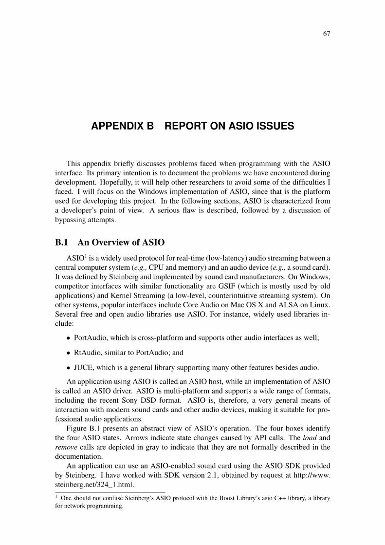
67

APPENDIX B REPORT ON ASIO ISSUES

This appendix briefly discusses problems faced when programming with the ASIOinterface. Its primary intention is to document the problems we have encountered duringdevelopment. Hopefully, it will help other researchers to avoid some of the difficulties Ifaced. I will focus on the Windows implementation of ASIO, since that is the platformused for developing this project. In the following sections, ASIO is characterized froma developer’s point of view. A serious flaw is described, followed by a discussion ofbypassing attempts.

B.1 An Overview of ASIO

ASIO1 is a widely used protocol for real-time (low-latency) audio streaming between acentral computer system (e.g., CPU and memory) and an audio device (e.g., a sound card).It was defined by Steinberg and implemented by sound card manufacturers. On Windows,competitor interfaces with similar functionality are GSIF (which is mostly used by oldapplications) and Kernel Streaming (a low-level, counterintuitive streaming system). Onother systems, popular interfaces include Core Audio on Mac OS X and ALSA on Linux.Several free and open audio libraries use ASIO. For instance, widely used libraries in-clude:

• PortAudio, which is cross-platform and supports other audio interfaces as well;

• RtAudio, similar to PortAudio; and

• JUCE, which is a general library supporting many other features besides audio.

An application using ASIO is called an ASIO host, while an implementation of ASIOis called an ASIO driver. ASIO is multi-platform and supports a wide range of formats,including the recent Sony DSD format. ASIO is, therefore, a very general means ofinteraction with modern sound cards and other audio devices, making it suitable for pro-fessional audio applications.

Figure B.1 presents an abstract view of ASIO’s operation. The four boxes identifythe four ASIO states. Arrows indicate state changes caused by API calls. The load andremove calls are depicted in gray to indicate that they are not formally described in thedocumentation.

An application can use an ASIO-enabled sound card using the ASIO SDK providedby Steinberg. I have worked with SDK version 2.1, obtained by request at http://www.steinberg.net/324_1.html.1 One should not confuse Steinberg’s ASIO protocol with the Boost Library’s asio C++ library, a libraryfor network programming.

68

Initializeddriver allocated

Preparedbuffers allocated

Runningaudio streaming

init start

stopexit

load

remove

create buffers

dispose buffers

Loadeddriver selected

Figure B.1: ASIO operation summary.

An initial analysis of the SDK’s contents clearly points out that:

• There is no guide on how to build an ASIO host. However, there is a referencemanual presenting and describing the API. This reference, though, lacks some de-tails of implementation—e.g., it does not describe the loadAsioDriver call, whichis fundamental to use ASIO; and

• The source code is not clearly organized. Maybe due to lack of description on howASIO host systems are structured, finding out the actual intent of each module wasnot trivial. Subjectively judging, the code also does not seem very readable in somesections, which increases maintenance difficulty.

Since the code is not self-descriptive enough to cover up drawbacks in the documen-tation, the reliability of ASIO hosts is somehow reduced, increasing the chance of unex-pected bugs. Since ASIO is generally only used by corporations, there is also very littleinformal support available on the Internet. In the following section, I report a flaw withwhich I had to deal while working with ASIO.

B.2 The Process Crash and Lock Problem

This problem arose whenever the ASIO host process was terminated for some reason.It could be terminated by Visual Studio (when stopping debugging), by the operatingsystem (through the Task Manager) or by either of those if it crashed for any reason(an unexpected exception, an invalid pointer access, etc.), which is normal and expectedduring a development process. In Windows, an ASIO host communicates with an ASIOdriver using a COM interface2. When the host process crashed, it was terminated withoutreleasing certain resources, probably the COM object instance used by ASIO. For a reasonI and others have not discovered (but I believe it is related to COM), Windows did noteliminate the process from the process pool; the process remained apparently inactive.As a result, the executable file was in use and could not be modified and, consequently,the code could not be recompiled. Forceful termination such as by the Task Manager hadno effect. To continue development and modify the code, the machine would need to berebooted each time this problem appeared. If one just wished to run another copy of theprocess, the ASIO driver would still be in use by the last process instance, therefore alsomaking ASIO unavailable until rebooting.2 One should not confuse an interface for a Microsoft COM object with the COM port interface.

69

The reader may feel tempted to argue that it is the programmer’s responsibility toensure that the host does not crash, which is quite valid. Keep in mind, though, thatseveral errors are not directly identifiable, specially when designing new algorithms, andthat correction must hold only after the test stage.

To avoid this problem, I considered temporarily using the Windows MME audio inter-face and only used ASIO when most programming errors were already corrected. Then, Iinstalled the ASIO4ALL driver, which can be obtained at http://www.asio4all.com. Afterinstallation, I noticed that this problem would no longer occur, either using Creative’sASIO driver or the ASIO4ALL driver. I thoroughly tested all situations that previouslyled to this problem and found both drivers now worked properly. At this point, I stoppedlooking for an explanation, as this is probably a local problem that does not appear onother systems, and it is not my goal to determine exact causes for such failures, though amore formal examination should be performed in the future.

B.3 Summary

I have invested a considerable amount of time trying to fix the described issues, mainlybecause ASIO is the widespread default system for real-time audio streaming, and be-cause my most fundamental motivation is real-time audio output.

ASIO is much more difficult to use than the readily available MME interface. TheSDK is not “developer-friendly” as well. I invested a long time trying to resolve issues Ijust discussed, since my application depends entirely on the stability of the audio subsys-tem. In any case, it is not my responsibility, according to the goals of this work, to entersystems’ internals to fix their errors. I could only develop my code as stable as possiblesuch that situations that cause such instabilities in ASIO do not occur.

At last, after the “crash and lock” problem was resolved, I decided to use RtAudio3.0.33, since is is more likely to be stable, due to testing, than my own code accessing theASIO calls directly.

3 Any of the libraries listed on Section B.1 could have been used.

70

APPENDIX C IMPLEMENTATION REFERENCE

C.1 OpenGL State Configuration

OpenGL needs to be configured as follows to allow general purpose computation onthe GPU:

• Create an OpenGL rendering context. On Windows, this is performed by callingwglCreateContext() and wglMakeCurrent(), generally right after having created awindow where graphics would be presented. In our application, window creation isnot completed, since it is not necessary—the framebuffer is not used, only textures;

• Check hardware support for extensions. Before we proceed, we need to know: themaximum texture size, whether the framebuffer object extension (JULIANO et al.,2006) is supported and how many attachments are supported per framebuffer object(FBO);

• Generate one FBO and two or more same-sized textures and attach them to theFBO;

• Load the shaders used for audio processing; and

• Ensure that the following features are disabled: LIGHTING, COLOR_MATERIAL, MULTISAMPLE, POINT_SMOOTH, LINE_SMOOTH,POLYGON_SMOOTH, CULL_FACE, POLYGON_STIPPLE, POLYGON_OFFSET_POINT, POLYGON_OFFSET_LINE, POLYGON_OFFSET_FILL,POST_CONVOLUTION_COLOR_TABLE, POST_COLOR_MATRIX_COLOR_TABLE, HISTOGRAM, MINMAX, COLOR_SUM, FOG, SCISSOR_TEST,ALPHA_TEST, STENCIL_TEST, DEPTH_TEST, BLEND, DITHER, LOGIC_OP, COLOR_LOGIC_OP, AUTO_NORMAL;

• Ensure that the following features are enabled: TEXTURE_1D, TEXTURE_2D;

• Set the shading model to SMOOTH and set the polygon mode to FILL for facesFRONT_AND_BACK;

• If clearing is desired, set the clearing color to 〈0, 0, 0, 0〉; and

• Provide identity mapping, such that texture coordinates indicate exactly the matrixpositions on texture bitmaps. This is achieved by doing the following:

71

– Set up a two-dimensional orthographic viewing region from 〈0, 0〉 to 〈Tw, Th〉,where Tw and Th refer to the width and height of the textures assigned to theFBO;

– Set up an identity modelling transformation and an identity texture transfor-mation and apply on both a translation on each axis (except by z) of 0.5—thisis done because memory positions are assigned, by definition, to the center ofpixel cells; and

– Set up the viewport transformation with the position parameters referring to〈0, 0〉 and the size parameters referring to 〈texture width, texture height〉.

Blending is disabled because OpenGL clamps luminance values into the [0.0,1.0]range if it is enabled. At this point, the application has at least 2 texture names and 1 FBOwith those textures attached to it. OpenGL provides a call to change the target texture,glDrawBuffer(), that takes as arguments not the texture names, but identifiers representingtextures bound to an FBO. Source textures can be defined passing uniform parameters—i.e., not subject to interpolation—to fragment shaders. Performing these operations manytimes is error-prone due to the different mechanisms of reference to textures. One canwrite a procedure to perform swapping of source and target textures automatically.