a goodness of fit test for bivariate normal distributions. ·...

A GOODNESS OF FIT TEST FOR

BIVARIATE NORMAL DISTRIBUTIONS

James Edward Mi 1 ler

LIBRARYNAVAL POSTGRADUATE SCHOOLMONTEREY, CALIF. 93940

United StatesNaval Postgraduate School

THESISA GOODNESS OF PIT TEST FOR

BIVARIATE NORMAL DISTRIBUTIONS

by

James Edward Miller

April 1970

Tki& document hcu> been appAavtd ^on. public kz-

IzaAz and 6aZz; aX& dUtu.bation l& untimLte.d.

I 1 J y _t

A Goodness of Pit Test for

Bivariate Normal Distributions

by

James Edward MillerLieutenant Colonel, United States Marine Corps

B.S., University of Utah, 1964

Submitted in partial fulfillment of therequirements for the degree of

MASTER OF SCIENCE IN OPERATIONS RESEARCH

from the

NAVAL POSTGRADUATE SCHOOLApril 1970

c

ABSTRACT

This paper is an investigation of a goodness of fit

test for bivariate normal distributions. The test pro-

cedure is based on random linear functions of bivariate

normal random variables. The test makes use of the maximum

Kolmogorov D(M) statistic over the linear functions which

are computed. An estimate of the distribution of M is

obtained by computer simulation. No attempt is made to

determine the power of the test.

IPTGPADUATE SCHOOD

[, CALIF. 9394Q

TABLE OF CONTENTS

I. INTRODUCTION 7

II. THEORY 10

III. EMPIRICAL RESULTS 18

IV. RANDOM VARIABLE GENERATION 23

V. SUMMARY AND CONCLUSIONS 27

COMPUTER PROGRAM 32

BIBLIOGRAPHY 39

INITIAL DISTRIBUTION LIST 40

FORM DD 1^73 41

LIST OF TABLES

I. Distribution (Relative Frequency) ofKolmogorov-Smirnov Statistics that Resultfrom 100 Linear Combinations of 100Bivariate Random Vectors from TwoBivariate Normal Distributions 29

II. Distributions (Relative Frequency) of 500Maximum Kolmogorov-Smirnov Statistics,Each of which was Derived from 25Linear Combinations of Samples fromVarious Bivariate Normal Distributions 30

III. Distribution (Relative Frequency) of 500Maximum Kolmogorov-Smirnov Statisticsfor Samples Drawn from Various BivariateNormal Distributions with IdenticalCorrelation Coefficient, p 31

I. INTRODUCTION

An important application of Statistics is to attempt

to find a specific probability distribution which fits an

observed sample of data. A well fitting distribution can

then be used to predict values of future occurrences,

relative frequencies of future occurrences, etc. There

are numerous methods available for testing the goodness

of fit of data in scalar form to a hypothesized univariate

probability distribution. Among these are the Chi-square

and the Kolmogorov-Smirnov tests, of which the Kolmogorov-

Smirnov test is considered the more powerful [1] . Further-

more the Kolmogorov-Smirnov test exhibits the very

attractive characteristic that it is based on a statistic

which has a distribution of the random variable being

sampled.

However, there appears to be a lack of methods for

testing the fit of hypothesized multivariate distributions

to multivariate data (observations in vector form).

Furthermore, no statistic which has the desirable character-

istic of being distribution free and which can be used in

multivariate goodness of fit tests has been found. In

fact, no such statistic may even exist. For instance,

Simpson [2] has shown an example of continuous bivariate

distributions for which the analog of the Kolmogorov-

Smirnov statistic is dependent on the underlying distribution.

Rosenblatt [3] discusses a possible test which involves

a transformation of an absolutely continuous k-variate

distribution into the uniform distribution on the

k-dimensional hypercube« The transformation is uniquely

determined by the theoretical distribution against which

the sample is to be tested. Then the transformed sample

may be tested against the uniform distribution in

k-dimensions . There are several disadvantages to this

procedure, however. For example, the results are influenced

by the manner in which the components of the observed

vectors are ordered.

The purpose of this paper is to describe a goodness of

fit test for testing a bivariate normal distribution (with

given mean and covariance matrix) against samples of bi-

component data. The test results in acceptance or rejection

of the hypothesis that F„ = F, where F„ is the cumulative

distribution function of the population of the bivariate

sample vectors and F is the hypothesized cumulative distri-

bution function. The notation in this paper closely follows

the notation used by Anderson [4], It Is expected that the

test developed here for the bivariate normal distribution

can be extended to the case of the k-variate normal distri-

bution. This paper is restricted to a consideration of

testing the fit of samples to a distribution which has

zero mean. This restriction causes no loss of generality

since any distribution with a finite mean can be translated

to mean zero by a linear transformation.

8

The goodness of fit test was developed according to the

following procedures

:

1) a characterization of the bivariate normal distri-

bution is used to develop a test statistic M for use in a

goodness of fit test,

2) the distributional properties of M are investigated

by computer simulation.

II. THEORY

Since there appeared to be no widely known statistic

for a reasonable goodness of fit test for multivariate

distributions in general, and the multivariate normal

distribution in particular, it seemed plausible that a

statistic suitable for a goodness of fit test might be

found by considering characterizations of the multivariate

normal distribution.

One property which characterizes a multivariate normal

distribution is given in the following theorem [4]

:

Theorem 1, A p-dimensional random variable X has a

p-variate normal distribution, if an only if every

linear function of X has a univariate normal distri-

bution .

The parameters of the univariate normal distribution can be

computed according to theorem 2.

Theorem 2. Let X (a column vector with p components)

be distributed according to N (y,E) a multivariate

normal distribution with mean (vector) u and covari-

ance (matrix) Z, and let C be a row vector of p

constants. Then

Y = CX

is distributed as univariate normal with mean Cy and

variance CZC (C is the transpose of C).

10

(NOTE: CX can be described as a linear combination of the

components of X.)

Prom the characterization of the multivariate normal

distribution given in theorem 1, it was felt that a suitable

goodness of fit test procedure might be to test the result

of a linear combination of the sample vectors (whose distri-

bution had been hypothesized as a specific multivariate

normal distribution) against the hypothesized theoretical

univariate normal distribution which has been computed for

the particular linear combination. Thus the problem is

reduced to the univariate level and use can be made of well

known univariate statistics which provide acceptable good-

ness of fit tests.

However, theorem 1 states that every linear combination

of multivariate normal random variables must be univariate

normal. Obviously one linear combination will not suffice

for a reasonable test. It is not difficult to envision

that there exists some linear function of nearly any vector

sample which will transform that vector sample into one

which is accepted as univariate normal. In fact, if the

marginal distribution of the components are univariate

normal, but the joint distribution is not multivariate

normal, the linear combination consisting of one component

(e.g. y = X-, + OX2

. . . + 0XN= X, ) is univariate normal. Thus

a test which uses only one linear combination might be

manipulated by the tester to give any results he desires.

11

On the other hand, it is clearly impossible to compute

every linear combination of a sample. As a compromise, it

was felt that a number (to be determined) of randomly

selected linear combinations would serve as a representa-

tive sample upon which an overall test statistic might be

based. To produce random linear combinations, the (column)

sample vectors were multiplied by a (row) vector of random

constants. The random components of the 'multiplying

vectors' were drawn from the uniform (0,1) distribution.

A uniform (0,1) distribution for the random multipliers

was used because:

1) Up to multiplicative constants, essentially any

linear combination of the components of the multivariate

vector could be produced using coefficients from the uniform

(0,1) distribution, and

2) A component of a random multiplier was equally

likely to be contained in any one interval in (0,1) as in

any other interval, provided the intervals were of equal

length. Thus there should be no specific interval contain-

ing a 'concentration' of the multipliers which might

adversely influence the performance of the goodness of fit

test

.

NOTE: The results of the goodness of fit test described

in this paper using random multipliers from a uniform (0,1)

distribution were the same as results obtained using random

multipliers from a uniform (-2,2) distribution.

12

The Kolmogorov-Smirnov test was employed to determine

acceptance (or rejection) of the hypothesis that the

linear combinations of bivariate sample vectors are from

the (computed) theoretical univariate distributions noted

in theorem 2. As noted previously, the Kolmogorov-Smirnov

test is considered more powerful than the Chi-square test.

Of course, the distribution free characteristic of the

Kolmogorov D statistic applies in particular to linear

combinations of the components of multivariate normal

random variables. A description of the Kolmogorov-

Smirnov test is presented in the following paragraphs.

One method of testing the simple hypothesis, H: F., = F,

where F^ is the cumulative distribution of the population

sampled and F is the theoretical continuous distribution

proposed for the population, is the Kolmogorov D statistic

[5]. The asymptotic distribution of D was investigated by

Kolmogorov and tabulated by Smirnov [6] and, for small

sample sizes, by Massey [7].

The Kolmogorov D statistic is derived from the sample

cumulative distribution function, SN , and the proposed

theoretical cumulative distribution function, F, as follows;

Let Y,,...YM be a random sample from a continuous population

with cumulative distribution function F. Let Z-,,...Z„ be

the ordered statistics of Y, so that

-co < Zl < z2

< ... < zN

<

13

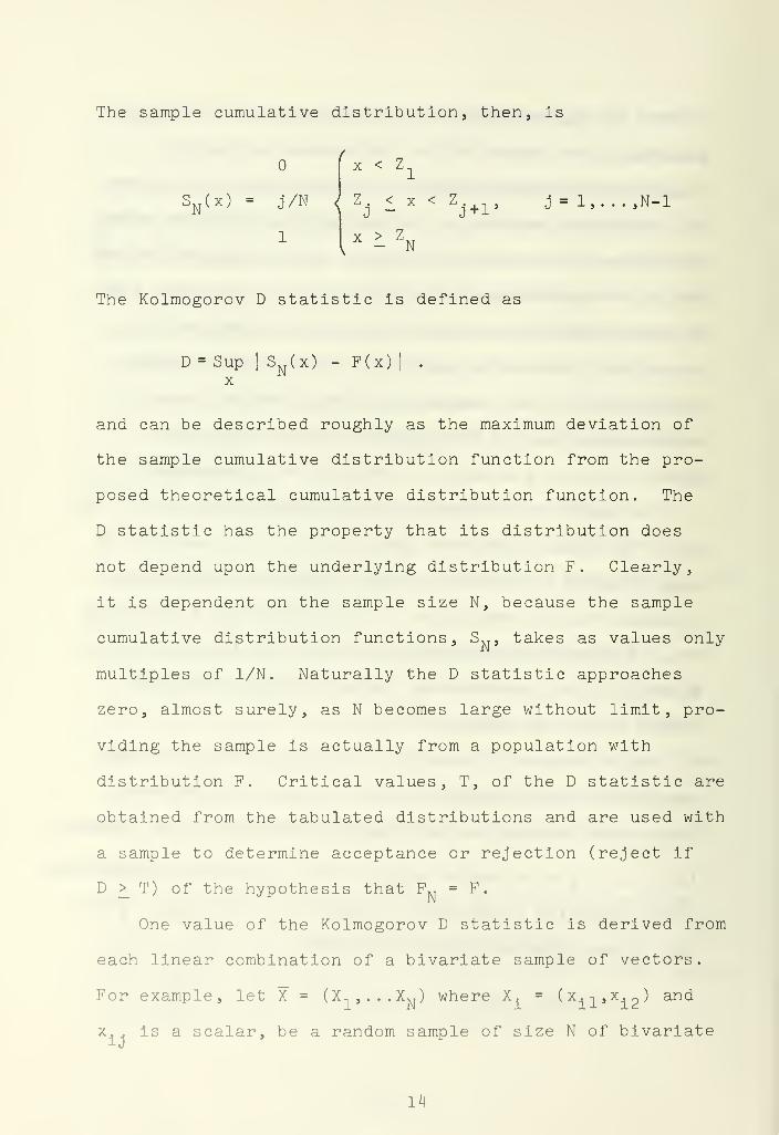
The sample cumulative distribution, then, is

SN(x) = J/N

1

< Z.

< Z1

< x < Z , j = 1,...,N-1

> ZN

The Kolmogorov D statistic is defined as

D = Sup|

SN(x) - P(x)

x

and can be described roughly as the maximum deviation of

the sample cumulative distribution function from the pro-

posed theoretical cumulative distribution function. The

D statistic has the property that its distribution does

not depend upon the underlying distribution P. Clearly,

it is dependent on the sample size N, because the sample

cumulative distribution functions, S„, takes as values only

multiples of 1/N. Naturally the D statistic approaches

zero, almost surely, as N becomes large without limit, pro-

viding the sample is actually from a population with

distribution F. Critical values, T, of the D statistic are

obtained from the tabulated distributions and are used with

a sample to determine acceptance or rejection (reject if

D > T) of the hypothesis that FN

= F.

One value of the Kolmogorov D statistic is derived from

each linear combination of a bivariate sample of vectors.

For example, let X = (X,,...XM ) where X. = (x,^,x.p) and

x . . is a scalar, be a random sample of size N of bivariate

14

random vectors. A linear combination Y = CX, where

C = (c-,,Cp) and c. is a scalar, is a vector of N scalars,

(Y., s . . . Y„) . Let Z be the hypothesized covariance matrix

of the distribution of X. To obtain a rough test of the

hypothesis that the distribution of X is bivariate normal

with covariance matrix E (and mean zero), one may test the

hypothesis that Y = CX is distributed as univariate normal

with variance CZC' (and mean zero). A Kolmogorov-Smirnov

test to determine the acceptance of the hypothesis when

one particular value of C, say C, is used to compute a

linear combination will yield one value of D, that is

D = Sup|FT(y) - S*(y)|

y

where Fy is the hypothesized univariate normal cumulative

distribution of Y and S^ is the sample cumulative distribu-

tion of the transformed sample. When the procedure listed

above is repeated for a different value of C, say C., then

another value of D, which may or may not be identical to

the first value, is obtained. If every value of D obtained

with various values of C is less than the critical value of

D for the given sample size and level, then the hypothesis

is accepted. Likewise if every value of D obtained from

using various values of C is greater than the critical

value, then the hypothesis is rejected. However, some

linear combinations of typical samples from a bivariate

normal population can be expected to give values of D

15

exceeding the critical value while other linear combinations

may give values of D less than the critical value. To

eliminate the ambiguity of such results, another statistic

must be used, preferably one whose distribution function

can be readily tabulated or computed. For this purpose we

use the maximum of the D statistics, M, derived from

Kolmogorov-Smirnov tests of a large number, m, of linear

combinations of the sample. That is,

M=max sup |SC j (y) - F*(y)| i = 1,2,. ..m

i y 1

where S„ y is the sample cumulative distribution functioni

of the linear combination C.X and F.(y) is the hypothesized

theoretical cumulative distribution of the linear combina-

tion C.X.1

The values of the D statistics derived from linear com-

binations of a particular sample appear to be more highly

dependent on the sample than on the random multiplying

vectors (see Section III, Empirical Results). Therefore

the maximum D might be expected to be a result of only the

sample so that rejection or acceptance of the hypothesis

H: F.. = F , where FN is the cumulative distribution function

of the population sampled, and F is the proposed theoretical

cumulative distribution function, would depend only on the

bivariate sample.

The distribution of M, as defined above, appeared to

be intractable to get in closed mathematical form. However,

16

the properties of the distribution of F were investigated

for several cases by examining empirical data obtained from

computer simulation. The data was produced by generating

samples of a specified bivariate normal distribution, com-

puting random linear combinations of the sample vectors,

and recording the maximum of the resulting Kolmogorov D

statistics. This procedure was repeated to give several

lists of 500 values of M. Each list of 500 values of M

was derived from bivariate sample vectors with different

underlying bivariate normal distributions. The empirical

results and generating techniques are discussed in Sections

III and IV.

17

III. EMPIRICAL RESULTS

In order to obtain the empirical data to study the

distribution of M, the maximum D statistic, a computer

program was written to accomplish the following for

specific selections of the covariance matrix, E:

1. Generate a sample of desired size of bivariate

normal random vectors from the given distribution,

2. Generate the desired number of multiplying vectors,

each of which would produce one linear combination of the

sample vectors,

3. Compute the linear combinations of the sample

vectors by vector multiplication,

4. Perform a Kolmogorov-Smirnov test on each univariate

sample obtained as a result of a linear combination and

record the resulting value of D. The values of

D = sup |SN(x) - P(x)

x

when S^ and F are functions previously defined, were

determined at values of .OIK (K = 1,...100) for the proposed

theoretical distribution P. For example, the value of the

sample cumulative distribution, SN(x), was evaluated at each

point x. where F(x.) was multiple of .01, D being assumed

to be the maximum value of the 100 differences

sN ( Xl ) - P( Xl )

18

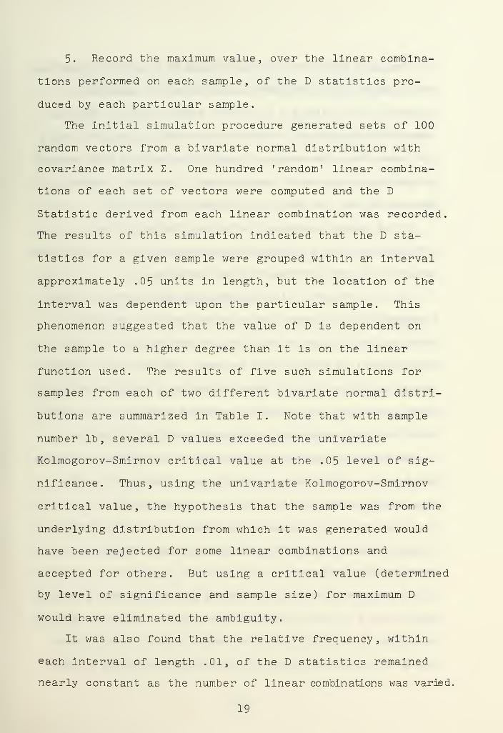
5. Record the maximum value, over the linear combina-

tions performed on each sample, of the D statistics pro-

duced by each particular sample.

The initial simulation procedure generated sets of 100

random vectors from a bivariate normal distribution with

covariance matrix E. One hundred 'random' linear combina-

tions of each set of vectors were computed and the D

Statistic derived from each linear combination was recorded.

The results of this simulation indicated that the D sta-

tistics for a given sample were grouped within an interval

approximately .05 units in length, but the location of the

interval was dependent upon the particular sample. This

phenomenon suggested that the value of D is dependent on

the sample to a higher degree than it is on the linear

function used. The results of five such simulations for

samples from each of two different bivariate normal distri-

butions are summarized in Table I. Note that with sample

number lb, several D values exceeded the univariate

Kolmogorov-Smirnov critical value at the .05 level of sig-

nificance. Thus, using the univariate Kolmogorov-Smirnov

critical value, the hypothesis that the sample was from the

underlying distribution from which it was generated would

have been rejected for some linear combinations and

accepted for others. But using a critical value (determined

by level of significance and sample size) for maximum D

would have eliminated the ambiguity.

It was also found that the relative frequency, within

each interval of length .01, of the D statistics remained

nearly constant as the number of linear combinations was varied.

19

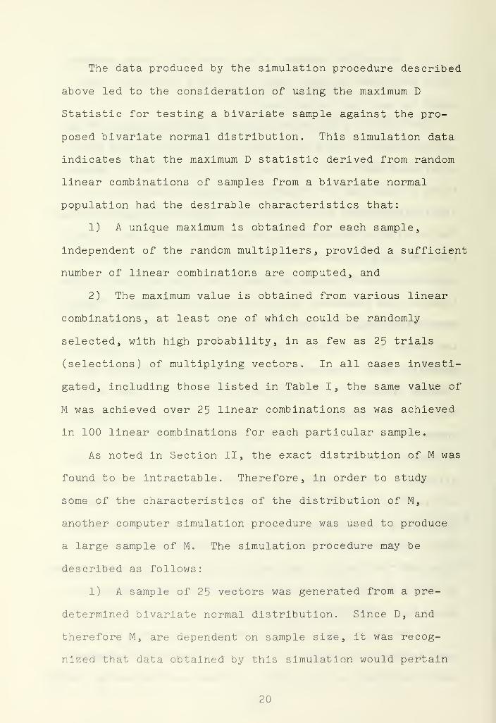
The data produced by the simulation procedure described

above led to the consideration of using the maximum D

Statistic for testing a bivariate sample against the pro-

posed bivariate normal distribution. This simulation data

indicates that the maximum D statistic derived from random

linear combinations of samples from a bivariate normal

population had the desirable characteristics that:

1) A unique maximum is obtained for each sample,

independent of the random multipliers, provided a sufficient

number of linear combinations are computed, and

2) The maximum value is obtained from various linear

combinations, at least one of which could be randomly

selected, with high probability, in as few as 25 trials

(selections) of multiplying vectors. In all cases investi-

gated, including those listed in Table I, the same value of

M was achieved over 25 linear combinations as was achieved

in 100 linear combinations for each particular sample.

As noted in Section II, the exact distribution of M was

found to be intractable. Therefore, in order to study

some of the characteristics of the distribution of M,

another computer simulation procedure was used to produce

a large sample of M. The simulation procedure may be

described as follows:

1) A sample of 25 vectors was generated from a pre-

determined bivariate normal distribution. Since D, and

therefore M, are dependent on sample size, it was recog-

nized that data obtained by this simulation would pertain

20

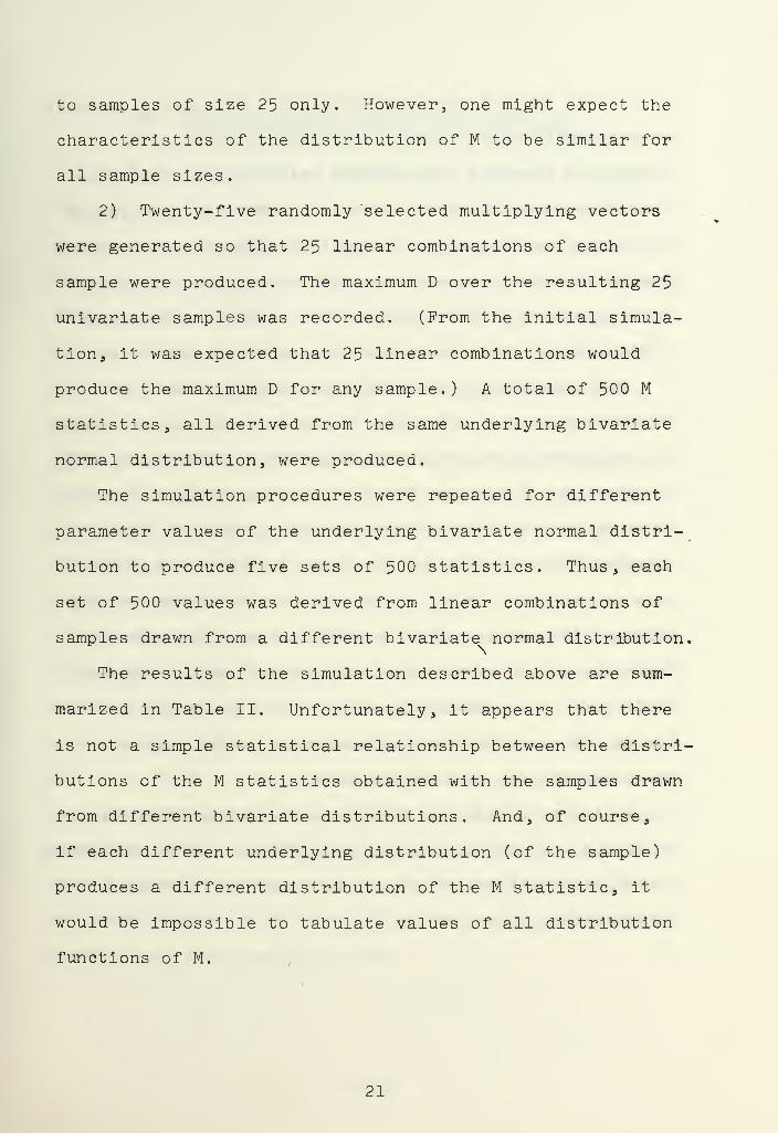
to samples of size 25 only. However, one might expect the

characteristics of the distribution of M to be similar for

all sample sizes.

2) Twenty-five randomly selected multiplying vectors

were generated so that 25 linear combinations of each

sample were produced. The maximum D over the resulting 25

univariate samples was recorded. (From the initial simula-

tion, it was expected that 25 linear combinations would

produce the maximum D for any sample.) A total of 500 N

statistics, all derived from the same underlying bivariate

normal distribution, were produced.

The simulation procedures were repeated for different

parameter values of the underlying bivariate normal distri-

bution to produce five sets of 500 statistics. Thus, each

set of 500 values was derived from linear combinations of

samples drawn from a different bivariate normal distribution.

The results of the simulation described above are sum-

marized in Table II. Unfortunately, it appears that there

is not a simple statistical relationship between the distri-

butions of the M statistics obtained with the samples drawn

from different bivariate distributions. And, of course,

if each different underlying distribution (of the sample)

produces a different distribution of the M statistic, it

would be impossible to tabulate values of all distribution

functions of M.

21

It did not seem unlikely that a similarity or other

relationship existed between the distributions of M

statistics obtained from samples which were derived from

bivariate normal distributions with identical correlation

coefficients. Therefore, a final simulation procedure was

repeated, using samples drawn from several non-identical

bivariate normal distributions with constant correlation

coefficients. The results are summarized in Table III.

Although there is a notable similarity between the

distributions of M statistics derived from bivariate normal

distributions with identical correlation coefficients (p),

the hypothesis that the distributions are identical was

rejected by a Kolmogorov-Smirnov test at the .05 level

of significance. This is also readily apparent for the

case in which p = .3162. Note that the difference in the

means of the samples of M is .0059, whereas one standard

deviation of the mean (computed from the sample standard

deviation) is approximately .0022. Thus the means are

nearly three standard deviations apart, which suggests that

the distributions are not the same.

An interpretation of these results and how they may be

applied to a possible goodness-of-fit test for the bivariate

normal distribution is discussed in Section V, Summary and

Conclusions

.

22

IV. RANDOM VARIABLE GENERATION TECHNIQUES

In order to study the distribution of the M statistics

described in Sections II and III, it was necessary to

produce a large number of random variables from various

bivariate normal distributions. There are several possible

methods which might be used to generate the bivariate

normal random variables on a computer. One method would

be to generate independent normal random variables and

perform an appropriate transformation on them which will

produce a bivariate normal random vector. For example, to

generate random vectors from a bivariate normal distribu-

tion with mean zero and covariance matrix Z, where Z is

symmetric and positive definite, one could use the follow-

ing procedure.

1) Generate two independent random variables, from a

normal (0,1) distribution, so that X = (X-.,X„) is bivariate

normal (0,1) where I is the identity matrix.

2) Perform the transformation Z = CX, where C satisfies

CC = Z. Then Z = (Z,,Z2

) is bivariate normal (0,Z).

In this study the bivariate normal random vectors were

generated using a conditional distribution approach. It

is a well known characteristic of the bivariate normal

distribution that if X = (X, ,X?

) is distributed bivariate

normal (u,Z) where y=(u,,Up) and

23

a12

a12

a21

a22

then Xp is distributed univariate normal (Up,<jpp). It

is also well known that the conditional distribution of

X.. , given Xp = Xp is univariate normal

[u-,+a-,papp (Xp-yp ) ,a.. .. -a.. pOp" a p-i] • Therefore, after

generating X?

from a univariate normal (Up,cjpp) distribu-

tion, the conditional distribution of X, , given Xp = x? ,

was computed and X-. was then generated from that univariate

normal distribution.

To verify that this produces a random vector with the

characteristics of the given bivariate normal distribution,

consider the following:

Let y = (0,0) = (\i1,U

2)

Generate X?

= x?

from its marginal distribution, N(0, Opp).

Then,

E(X2

) =

and

E[(X2

- y 2)

2]

= E[(X2

)

2] = c

22

Generate V, independent of Xp, from univariate normal

(0,1) distribution.

Now

E(V) = 0, and

E(V 2) = 1

24

-1 3* -1Now let X

1 = ( a-i -i

— an p

a22 a 21^

2 V + °12 a22 ^ X 2^*

X, is univariate normal (o-.~°?n~ (X? ), a-.^-a^~a~ a

?1 ) , and

E(X1

) = E[(o11

-o12

o2

~ 1o21 ) V + a

12a2

~ 1(X

2)] = = y

1

Similarly, the covariance between X.. and X?

is

Cov(X]_,X

2) = E[(X

1-y

1)(X

2-y

2)] = EU-^)

-1 h -1= E{ [(o

11-a

12o22

o21 )

2 V + cj12

q22

(X2)]X

2>

—

1

h -1= ( a 11

-a12

a22

a 21')

2 E ( v ' x2

) +a i2a22

E ^ X2^*

Since V and X?

are independent,

E(V • X2

) = E(V)E(X2

) = 0.

Continuing from above,

Cov(X.,,X2

) = + o-.2

<j22 (a 22 ) = a-,- = o

2-.

The variance of X-. is

E[(X1

- yx

)

2]

= E(X2

)

"1"I Q

= E{[ (o 11

-o12

o?

~ ±o21

)^ V + cf

1 2a 22 ^ X2^ *

-1 2 —1 J"=

^ a il~°12a22

a2i^

E ^vL"^ + (

^ a ii"ai2

a22

a2i^

E^

(a12

a22

1) E(X

2) + (o

12a22

1)

2E(X

2

2)

= o11

-a12

a2 ;

1c21

+ °12

c2 l

1°12

= ai;L

,

since o^2

= o2

~ .

25

Incidentally, this technique can be extended to a method

of generation of p-component multivariate normal random

variables, since the distribution of X . (i=l ,2 , . . . p) given

any X. = X . ( j = l ,2 , . . . p , j¥i) , is also a normal distri-j J

bution whose parameters may be computed.

Standard computer routines were used to generate the

univariate normal and uniform random variables required for

the simulation procedure previously described. The routines

are shown in the computer program under Subroutine RANDU,

(for uniform random variables) and Subroutine GAUSS (for

univariate normal random variables).

26

V. SUMMARY AND CONCLUSIONS

The empirical data indicates that the distribution of

the maximum of the D statistics (M) , derived from Kolmogorov-

Smirnov tests of linear combinations of samples from

bivariate normal distributions, was dependent upon the

covariance matrix of the underlying distribution of the

sample. Therefore it would be impossible to tabulate the

distribution of M except for specific parameters of the

underlying distribution.

However, a goodness of fit test for the bivariate nor-

mal distribution can be constructed using the M statistic.

The test might consist of using a simulation procedure,

similar to that used in this paper, to produce a sample

distribution of M. This distribution of M would be derived

from samples which are from a bivariate distribution

identical to the proposed hypothesized bivariate distribu-

tion. Then a critical value of M, for a test with level

of significance a = a , may be established as the value at

which the (1 - a ) percentile point of the distribution

of M occurs. Obviously the number of linear combinations

and the number of M statistics for development of the

sample distribution of M must be determined by the experi-

mentor performing the test. (Note that the size of the

samples generated in the simulation procedure must be iden-

tical to the size of the sample to be tested.

27

For example, suppose one wishes to test the hypothesis

that a sample of N vectors was drawn from a population whose

5 2distribution is bivariate normal (0,1) where E = (_ _-)j

(one of the distributions for which M is tabulated in Table

II). If N = 25, then the distribution of the M statistics

is shown in Table II, listed under the appropriate covari-

ance matrix. For a = .05, the critical value of M is . 33 s

the value at which the .95 percentile point of the distri-

bution occurs. Then 25 random linear combinations of the

sample vectors would be computed and the 25 resulting uni-

variate samples tested against the computed univariate

distribution by a Kolmogorov-Smirnov test. If the maximum

of the 25 D statistics thus obtained is greater than . 33 s

the hypothesis is rejected. Otherwise the hypothesis Is

accepted.

There are obviously many interesting aspects concerning

this (and other) multivariate goodness of fit tests which

should be investigated. For example the power of the

test described in this paper, when applied to samples from

distributions other than the bivariate normal, might be

investigated. Also, a goodness of fit test based on a

statistic other than M (e.g., the mean or variance of D

obtained from linear combinations of the sample components)

might prove to be interesting. It is, of course, desirable

to find a "reasonable" statistic for which the distribution

may be found and tabulated.

28

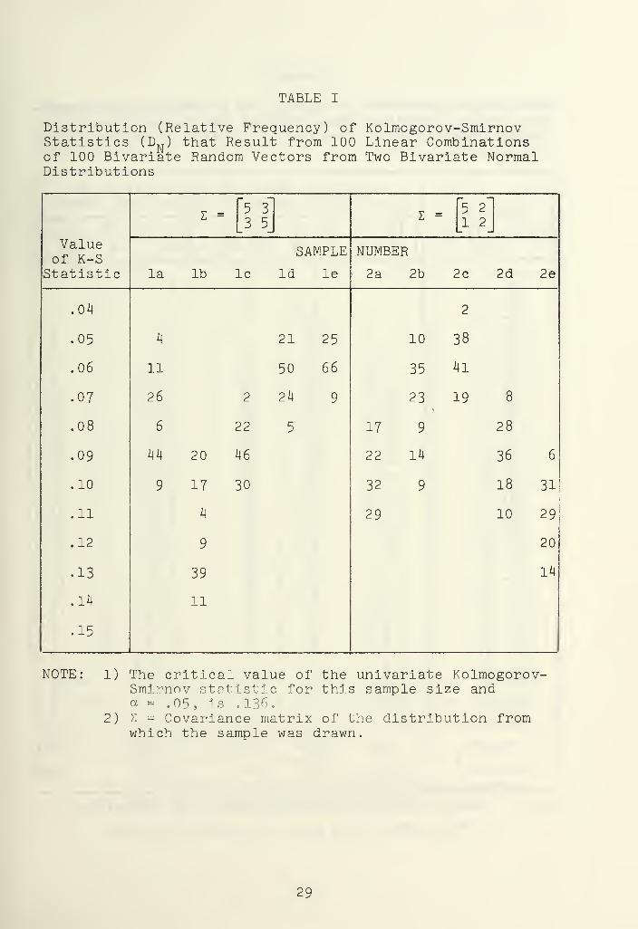
TABLE I

Distribution (Relative Frequency) of Kolmogorov-SmirnovStatistics (D^) that Result from 100 Linear Combinationsof 100 Bivariate Random Vectors from Two Bivariate NormalDistributions

Valueof K-S

£ ="5

3

_3 5_E =

"5 2"

1 2

SAMPLE NUMBER

Statistic la lb :Lc Id le 2a 2b 2c 2d 2e

.04 2

.05 4 21 25 10 38

.06 11 50 66 35 41

.07 26 2 24 9 23 19 8

.08 6 22 5 17 9 28

.09 44 20 J46 22 14 36 6

.10 9 17 30 32 9 18 33)

.11 4 29 10 29|

.12 9 20

.13 39 14

.14 11

.15

NOTE: 1) The critical value of the univariate Kolmogorov-Smirnov statistic for this sample size anda = .05, is . 136.

2) £ = Covariance matrix of the distribution fromwhich the sample was drawn.

29

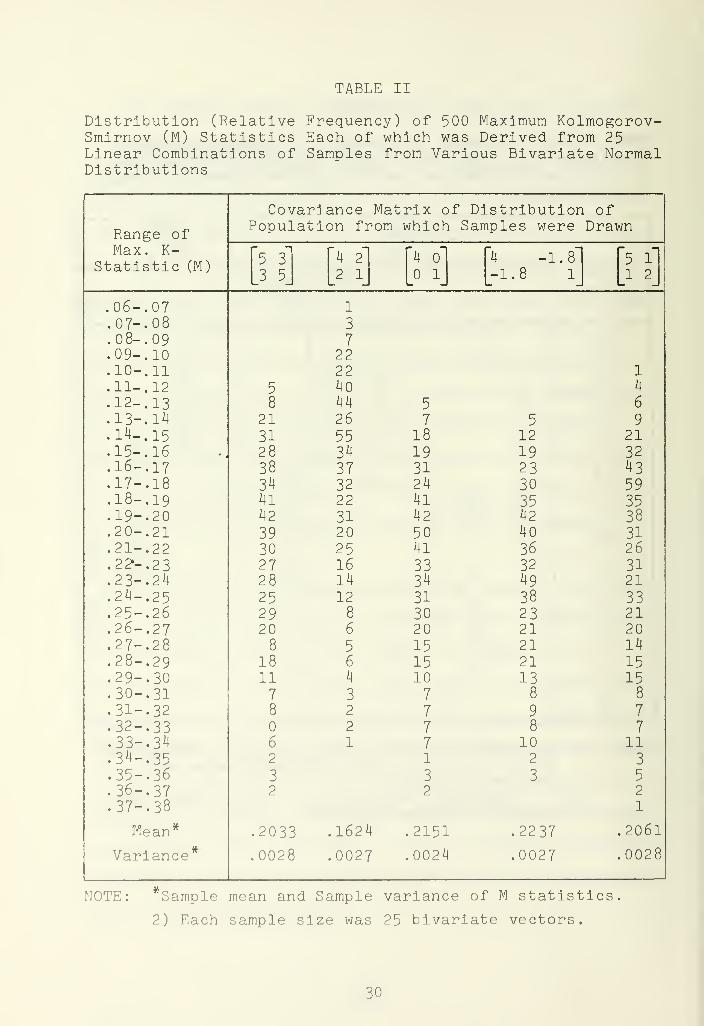
TABLE II

Distribution (Relative Frequency) of 500 Maximum Kolmogorov-Smirnov (M) Statistics Each of which was Derived from 25Linear Combinations of Samples from Various Bivariate NormalDistributions

Covariance Matrix of Distribution of

Range ofMax. K-

Statistic (M)

Population from which Samples were Drawn

^ 313 5

"4 2

2 1

"4 o"

1

"4 -1,8"-1.8 1

"5 l"

1 2V--il__Jl__Jl_ _l l_ _J

.06-. 07 1

.07-. 08 3

.08-. 09 7

.09-. 10 22

.10-. 11 22 1

.11-. 12 5 40 4

.12-. 13 8 44 5 6

.13-. 14 21 26 7 5 9

.14-, 15 31 55 18 12 21

.15-. 16 28 34 19 19 32

.16-. 17 38 37 31 23 43

.17-. 18 34 32 24 30 59

.18-. 19 41 22 41 35 35

.19-. 20 42 31 42 42 38

.20-. 21 39 20 50 40 31

.21-. 22 30 25 41 36 26

. 2 ?- . 2 3 27 16 33 32 31

.23-. 24 28 14 34 49 21

.24-. 25 25 12 31 38 33

.25-. 26 29 8 30 23 21

.26-. 27 20 6 20 21 20

.27-. 28 8 5 15 21 14

.28-. 29 18 6 15 21 15

.29-. 30 11 4 10 13 15

.30-. 31 7 3 7 8 8

.31-. 32 8 2 7 9 7

.32-. 33 2 7 8 7

.33-. 34 6 17 10 11

.34-. 35 2 12 3

.35-. 36 3 3 3 5

.36-. 37 2 2 2

.37-. 38 1

Wean* .2033 .1624 .2151 .2237 .2061

Variance* .0028 .0027 .0024 .0027 .0028

NOTE: Sample mean and Sample variance of M statistics

2) Each sample size was 25 bivariate vectors.

30

TABLE III

Distribution (Relative Frequency) of 500 Maximum Kolmogorov-Smirnov Statistics (M) for Samples Drawn from VariousBivariate Normal Distributions with Identical CorrelationCoefficient, p

Corr.Coeff.(p) p = .6 P = o P

=S±°_ =. 3162w

10

Range^\^of M ^s

5 3 1 .6 4 1 5 1 1 . 3162

3 5 .2 1 1 1 1 2 .3162 1

.10-. 11 1 1

.12 5 3 4

.13 8 8 2 5 6 4

.14 21 18 3 7 9 8

.15 31 27 19 12 21 21

.16 28 51 31 31 32 29

.17 38 41 26 33 43 31

.18 34 38 25 46 59 26

.19 4l 51 39 55 35 44

.20 42 31 35 29 38 39

.21 39 26 38 37 31 41

.22 30 28 43 34 26 35

.23 27 27 45 31 31 33

.24 28 21 37 23 21 44

.25 25 26 23 24 33 15

.26 29 16 30 23 21 28

.27 28 25 22 26 20 16

.28 8 9 10 19 14 17

.29 18 16 21 13 15 18

.30 11 6 14 16 15 11

.31 7 9 11 7 8 9

.32 8 5 12 9 7 9

.33 j3 4 3 7 3

.34 6 1 1 2 11 4

.35 2 2 4 6 3 3

.36 3 5 4 6 5 3

.37 1 3 2 3 2

.38 1

Mean* .2032 .1998 .2168 .2130 .2061 .2120

Variance .0028 .0028 .0026 .0027 .0028 .0026

NOTE: 1) Mean and variable of M.

2) Sample size - 25 vectors.

3) E = covariance matrix or distribution of popula-tion from which samples were drawn.

31

OT ^.oo \— cLU < H-<

-J 2 • 1-a. c <J£ —1 UJ Uj o< 

—Ja

LUo

_io

Z£ QU

at •oo

2

LL i—

i

00 LUC ore LLI

o or<

UJX

OXLU

1— Uj<Z

LULL— z

I

Z > h» U^ aro -JOC M <o LU»—

«

Q.— >MM re a. LU«— Zoo «— 00 CD1— a 00 LLOO h-oo

2 3 UJ aroo o< _l< C 5 > Oo a:a =5 LL> Ct-J _J Cjc h-i-i at _) _j O— «•_>

i

cDT oo t- r < 00 •— Ir-OT ^or oa — 13 UL > OQC L><

LUor Octor ^^ X LU k-ac >i— — i—

UJ U'OT >—

1

X OOh- _ C-i oo\- XI- a 1— **»—• ^CC 3j LU~

i— oo i— KCC C or TCC _Ja »— < 00 <or D< o< cn

2: i^Q 2" OT I— <r z O <r

c UJ >v Ul oo <00 Z-00 »-m

o -_! UJ o t— OO TC < <<T or<— CC < •i LLO CV CO — LLO1-3 M o i— OO » o rv oo LL

i/jZ — or. • 2 — lf\ o 1— .-• m> ^-1 aLL. r\j < o UJ O 1- O u~ O 1— «~

>LU »> > * 5" o 00 LL r-t —LL O oou. O i-

Zk- r\j a o IX in «o —

.

_lO r-< —o O l>0

—< —

»

Ot/) • h- » -1 —

•

_J «—

<

>—

«

»—

«

x m <r z o LUZ z -—

'

_lJ- a. < LUO •> I— K uiO UJ IO 1— LUO<< r Xt- o oo < X-i > 1— -« -I X— K UJjC> o *-o e 1— KOO z oo 21 h-oO < X•j,— •—i UJ a \ < oo «£ < OO^ 3 ^r 2 h-OCC o~ oo> s, h- h- oOLU OT (—LU Of. ooa' XOT »—

*

< < —a: 5! — 21 ooQ- 1—

<

re •—

i

LO —

i

< <— > — _i »* i——O <s\ OZ on •—

.

oo »-LU 00 ZLU oo arm oO <Ii Z .-< X Z OOX z <x Z ui z T»— LL LU

c

1/131 <t—

Q

h- IUr»—

•

Q

l-t- UJ3T1—

•

Q

ori- LU oil— LL'

2:

O

X

OOOOOOO ODOOO OOOO K-iU>iJ)<^)^ OOOOO <^i-3<J)^<^> LJ^

32

oOUJ c_ t- "^_J 3" •*

cc < 5T a t

< l/)5 £ Uj <3 O -J— LL 5"

<J i'J UjL2 a —1 «•» ^ u.> CL C l-<X UJ ry •» or m Cj

Or <cr \- a at m z—

-

Qft Of CL <x u —

.

LU a LU UJ w- — rviy UJo t- »— Uj Zu; HN T" t~4 _j »*"* »-LL) < «CX LUX »~ 1- Q Cvj —

i

Q£K- Oh tr s 1—

1

•—tSJ bv4

Z ae. Li. LL U_ <rf 1— <_J or<t < zu. LULL > O or _J ra <tX > u.O era z C 3 C5 >

*—

•

ts ^^ z c 5 -.< ^-t

oO Z z oz c a: w 1/5 U) cr

< _ LUX h-D c •—> a »• — a..t— N— *- t— 1/3 — 00 U'

OOLL i— ooi- 3 i/j Z! > II 1 X3fS UJ CO ocr; c O i-H c •X »-

LU—

i

h-a *-C h- LL CC 1—1 cr'

_i jr UK _J*- LL 5- O'X LLI

Dui CrT UJ r> a !X Ul D •-—

(

-».*.-

51 OC o >or 2: LX. O *«J — ex: LUIX o oo •— •— r .

' 1-

5 O OO X-* ST*-i LU Or. LO CI -<C'_J z Cl Oa. a a < r-l?" 5:CO <t ca GQ. _J a ^J •M UJ Q. <—• ^ tj L5 —y:i/~ —

•

a Li/ '-TCLU *<0 ^ _J o? r^ >ljur- *>j KJ u 1—^ < —< Cit

.L.h- O x—

•

LL *- w> _J '/5 IJ_ oo^» CL »x< o O-J C_l < r-i

••or —- r—

1

i-st t-~ < < or — LU —

<

U-' ~ XX — _l a •— cr — lU h- X « f-^> X rsj <:

>• o X_) UJI— aii- xz •—

*

1— O •0 V- 1— •>

ou. o O0< COlari to— 5" 2! CJ- h-Z" —n_> <. rsj ••

dj m ujr 212 srz Jll U.I _J ta^ 1— u. ~- C^-iO^ —

»

CL -X. x>- X— zc t > 2IUI-. <Ilu u" C tr XHSJscz: o z z UJ zo ZliO 2! X ,~ cf <3 >SO > UJZ jj LU dJZcC CM »—- 0*- Z C' 2 Z •

i—— cc X ix.cn UJ CC xc1 -»- -«•• • "^» > 01- O XOoO CJ 1—3 X X t— •-n— r- 4 » 00 »^ —0 — •.!—

«

LL'^ ^i r- > h *- t— 1— hi/; irt* 00 — c: 1— JJ OO r—1—>UJ <r oo a iS) </3 i/>X coa-r-i— sDojco OfNJ II [X> —

'

s. >-<>- o 0^3 CloD •—cos: *-* X- h-*~ (\Jt- a II OOi. •—

I

2T < Z ti*r«S <:.—>>. IT Lf "v •»•—1 1/: >v JOV. s Q.T V—O 00X "> C :>z EK r-4 t—

t

1— crTh- •4-O^cc. fiMU •>"s» -> CJ ft •<—Xo •—1 Jf x oi_> K-l— II O-•< re,** O —•*-—' -c*- 000 3l «zuj 1/5 r~ Z II LULU II _J_I K-LOI~ r^ t-K 1- a. »^l— c *-.z 00 OCO<x Z 2:u_ O >> ?I 1— 1/5*-'l/l LU <TO UJ 

xt- LJ CJL ..- 5~ OZIZ *-zz < Z i^\Z. 11 1—5 !!>— i.<r h2 *-QC II —"_JI»_ 2 UJ _j h- *-x> —>cr on -or: r-» _J— Q > 5: OO xar. ac ejen r-^2 LX<*o o z z z *-3:u_-

1—

i

r*-

JCLLOO

•4- O

^<oo

O'OOO UUUOO OO OOO <-)<~><^ <^}<^><*J<^)<^) o o 00000

33

X «-l

K-uo » u_UJ -5 c -

oo >_J ^» l^—

•

o: cccc — h- »- o UJt-t UJ —

1

2(\) _J QCa -3 o _J or. X«— c C h- UJ i^ <5 h» o _J 41 X LL UJC5 _J 1X1 -~ 5: h- or.

i—

i

3 >•-< o —» 5"I/O T

510Q.

coo

ur.—

»

)< 5- a— * i—

i

•x(\J C C_l w h- H

•» — e z< —- «3 00 oo t_j>—

.

-~ 2* <3L rv 3" U' UJ »-^

•m* rvi <J act •» O h- k- h-u »- CX O —

i

•—> ooUJ r\j UJ2- •_ oo oo X ^*> —

«

UJ X o CNJ 1 O t-z - k > * U- h-ct O

0000UJk-

2 (\|—

»

<I5.

oo

* 00 UJ Of

•f ~5O0 C

or

oo

—

»

"V < GLOO + w or. u ^— ^jfJoo ^UJ — t- r^(V o UUZ -a: — f\l_l— u_ O UJ* t ?n ««i. —

t

* 5"liJ t •—

»

Xr\j —1 Uji-i X>Uj •b * C<_J UJ i— h-w —

'

OK SIX -5 -aZ Q. oo T t— —

.

3o <M <lO0 _J -5 -^ < < u—4 —

-

—

»

QCCCi ors: 5" •w— CL 1— U_' Ujoo <N (M OS" OOl o 1— f\Jh- CD '71 > 2T

•• > DO on c _i -oc C i~ _J\ .—i OCO 1U. > f\io Cto^ > Oi—< r\l Of _i _J Z r«~ioc<r _J or X• I"-3 5 U-<X u. IX UJ< —C'«-'2;v. 'J_J0 O < 5"

1—II^C <J iLu X ivi lof ^-•r-. i o X< o s:"^

—. «— l-Z l-h- » «.-—. 1- »— C: i— 5L

Deo » »—

t

•> -"C 1 O0" Q S" Mi

rf 1— r- > U-O t-O—K -~ w LL— i—

'

> Uj 3! Li. u_ < 5">UJC • I— ^r o^ 5"

f\jlL^~ •I ^O ?. - X •i KJ Z! 2^>CiH*> ^ Lu

r—'—. r i*- •—'O •.»-< li«—

1

II fc-nt » »<— <rjx f—< •» o —

»

x•—— I,-i.—<o/" H-CJ r-t—- w »— jj r-l—l^ri ? •> h-O 2 1-

(NJ< •^>— r—

1

ar.or. — — Qt "—

'

C 0~5 II Ci *• — h-

r •< OO - DO. II Z> .—

<

3 pg O-l • II 11 II «i> < <— O X oo OO— OK 51 1— oO—

•

a Q *.<> • aa. e h-O0t—

—

a _j *s UJ >—

i

—•>—(L5O0C3— Ul X mZ *—

<

Z i—

i

UJ •—i -»•—-o _J^-'JJ < s. t~

oo e— C>< 3 !/>U <> < > _5 ook n >—' • II 5. w 3 o0 5" oO X

O ^.i/iOO * _•—

1

rr\o£ — i ac»- i 2T H-._l Ovt-w a z i— or. UJ ^ <:tx> II

< UJ —• II o \- \— *—

4

12 X j-o - 1 uj or >— ro X 5"

> ~ II II _J>h- V- jt —

•

t II _i _i ii _j l~ K-5" < —*--«t— w o an— 1—

z

h> _J i—

iiTfM _JZ ^ I 5"_) > z: s: < 2-* rrz* —1-7 5. U-f^l- -•< <C Q<xr<rxo cr H coiu. rr Z'O <Tf_ < "-"CO oOO QT.O OU- a o>~IQT.O h- OOX— >— ncro o

—i O rnr- O o oo•—

<

r-

<

r-4 r^HUooooo i-)<J>Ui-}U o OOOOOOO oo

3*

r- — *OO • r- *

Cj I—

1

o • *z r~> o *<r

»u.

9-

i—

*

u.

•s-

LU 4 m •> *U> • * *

o z m —. ir. o- *LU*/ < LL in M »—

•

KZui 1—1 •» • VCv a:

<"

u.

ooLV *

oooo > • ^<-« •—

<

*_I_J UJ « h- K ><< •• O o^ ood- z • OO 1—

1

toH rfoo <r »—

<

1— >- #LULU LU' 00

OO<>— 1—

#*

lu »-- >—

4

o oo 00 •H

—J oooo LU t- 1—

<

uQ. t-t- X OO h- oO oo L'-

51 iC^ H^ t-* 001 1 iic

< O h- »—

1

x: * 4oo o. •. 00 •—

I

U)t- < X*

UJ r->~* H-oO oo 1— X < fr

X •. • O^- 1/) < ?" *l- OO 0l+-

2T<51

LJoO II

•X. + X t—

«OO orx (— 5-51 ? X • (X LU •r

LJ oo <r o < X <T a_ Q *_l 2Z II QCUJ OO 51 < c C; <f

«Y* OX z 5 X • Jf

<x oooo X Oh U- M -~ LU 5» >

H^ <:<r <r X —

.

IO 1— bi. 1 t- O LU LULU h- !U 00 *:lu —.00 2 OOO i—

i

• <<

hh i> H- a cr -12 < _J2 oc D >u_ iU —» (-O < fcTT O LU •_• <r>>- «C LULU X 2 M • 5 O 0-I+ Cr- 5" t~ < rj:>jjoo .*

o~? < U.U. O oo LU5T jZ O— < o< — < (Ti K

a UJLU 5" X OO OO z OO o^ ^—*l— OCCUJ OH O a cr.a-t— uj *LJU <X h- <r 3 --• • • oo (XLL- < •XX '-'OO ©OliflX -t(

cn h- 5" ZUJ a •k Z X •.-—I K 1— ^~« CO K- t- -*1

3T oo oo t— 0<X o 1—

«

— — t— ^-too«- —.- ••^** >-«- -^» — a

O i n • U- *-*%. r-Ht—

<

*: + o- f- r-l •• r-t—* «^ro »t r-»2 Li. H II u_ c- * II ^(rtj, "n. i— cr c> rro sf' •

>> o II C£LU II >s ->5" J)0 + •ur.i il + a? sO<^' CXN tfMToO ra. • o> * wO <\J _J 51 h- 5T 3 (— 1— -—

»

OO —

-

a— «a<r IX 1— oO ••(— OOSTO »\oo?^ oo ••'^ ••"v ^z? X UJ 2" li I i— -^-jo-JO^âjvD-v LU •_IOooO— 4i-JOoo 0*- 0«-LU-T«-

-

Of JSCOC <o->o o0< 1-~ 3 C 00 — c i/i II -» - o—

»

< ?2 jM 2 •-•-j or it II r- II (/I II >- z O II h- t\J II t- 1-2 1—

> LULU (—*- h- *—

•

XLL f- r- t~ t->LlJ< •—

1

II C> II LU<. II <r || > U.1< LU< i— U.<Iz •—*»—« —t-<t- H tx o5:jvOZ-zkk5; 1— *0 fXK-5. X ÛJI-Jh-^l- t-5

5j t— Z oo ~> oz'»-iX —75 -«X2 x<r C 1-'X '—X2 -•o-ULO l/J ooooooLou-oooaro^ OOOS-tXOOOO-CI-cr O:XX'O iXO«-iOWO QCtilJOZMÛlLL-iOoOO^(YSLLL>iaoO>^3:u. JLL030.

o r^ CT a, o »-< Ovl f, <t sf p-

t r- r» h- h- a > cr o a i-i

r-( o vC l sO *3 -o O -o <; «>- US

ououo UUUJU 1

ft.

1-2OOLU

oo

35

wX -X 3"

Li; UU-k 3 •-•.•> a LO_i < s: -4-o«o •> * mi*- C"a u- »0 •—> cMs*-LT\fMoc mc f- o5" 2!Z xc — •• «r^-cp • • ».f\i lull' o«a —c< <2T o »»•••• * ii» »>4 •> o • y^- X^ i—V < nx 2. or O m o> in * • »-m • ••»-- re in <f _*.<> K O 2^

t— - »— —< fNjroLnt-<h- nJ-o oonjmo^r- >t^«-< Q- jo< Oo— ujs: — • • af-cu rÔ" oor-trgm »>f #a • — c <*->

UJ2C IlA •.»«.«• vto (•«") ••.»* • *fVl XQ XH-7 h-xooo>- I > <Njao>* • • i • i » *>inr-* c\j «<*"> —a. oxC 4U.HZ > QC fMCOinO-O «-< • I ••(N|st'-< •" <*> fVJ U_ UJT

X co O • • af-cc i r— • ••vOo«v)a>ir> ô* » m »—i-ZJZ •>— •or 2T «.»»»« »f>sOfM(\jf\iir\ »© »oo a x i/>or:

oÔ<C •H»K O Oi r-ir^C"1 » » OON-^H • • »-4 »(\j<\i ot— —>i—jj_>i—« ao?"(-5 cvmmcîn ur\ »>o<J" • » »cr • r~- «m oot— t— uuh- 2:—o • • • avOco m»-t • • 1 r-*of-«-t m *rv i/ô —<-<x x »doj — •« • •>s. • t 1 I •r-crao * -4-vj- • uj,?' xc

> cc 00 cc rv. u, a. _j O o>Cf\J»-»-o—<•• »»-«—<>j ••—• •cv » x< »•O*-"*-**-1 O c; <\jcimco>4 I

no (>*->}- in • • *>t c\i>fr _j a.—2a. or, »CI^ «-" • • avOCD • »00-tr-i » (\jf"i *£> arc < Z .-t

or*— — .—ijso >* «••>•»• ••—iir> ar- • •f-Hf^<f • x »-<\j >o x »>-H/)2l/) »— XUJ «-CTLn»-l • •> »>fr.-t • I I LOvDODr-" «4 r-4 • — 00X^h/1n- 11 i/)X h- co r-«en in r-cOO^vO I I •> »—1-4- • •• eO •> It- ~—

•

t/)G o uj h- -J o • • •-©aooN • » »r-r- • • •rc^ -co 00 X—

J

l • *rxx i/i •**••• ••-<vtfT>«£>r- • »rôcO i-h «î •—z jc<.>~ZJ<-t-oi/) at »>a;.ô «•••

I f\jroj-r-<ÔOrvJO <M »rg XX 2Oi-*0<5^ << — r*-~*cnmowco »^-ir-- • »(m-^cd • • loct- • :xu_0 y-cccc »wOHU.ai o • • •nOooct*.-! • • 1 1 ^-<si" «r-i%o «o uj <cOOKhQD C •> #•.»»#• •^^»-•

I•.•.«••.»» »rOfr J— Q. h- 2T— cT-^-o*— • >— LU — *KmO» •• •• »f^- l nOcm • •-rvj^-r'i u> .ro <ui<l X

en fT-Jûu uxn O -Oi-trf>vtiO»-*r,~- « NO'OOOJNMrr'. sO »(\J h-X u.'

< 5<xxilo or o o • • •ooLO> »-<ir\r~vtrvj^-«^-ir-<\j • inoc • i-h/;_i u_x> j?u.t-nzoo —

• ••••••'•••i h-r- r • «vj- • ,cv ••- o < ok2T Oat: O lxjujo — »-v£)rvjTO » • •• t-* • 1 1 » • »»-4 • ».rf

N.^- »jj>^ c: o. Q- 1/^ at h- uj Lrr-tro^ô^^J • I » -<t> »c- »^" st #fv _)uj 00a.

•• ?"uj>-iuuj<q- r.i O • • •vCXOorjr-i ».>tt*-fs- >cr<-»irMr\ <n • • u_a ujcx < >—X—iu-X t— »»»•-•• »oo 1 r--<Njrv)t.jocr-pô otc •• 0200 xu. Q.u._Jt/) oo »i^hN » •. # o lO<N «f0 ••—• • e<MvO <»-h —I

2 iy;X C>— ^-<»— h- 4'•-^f^l•4'^0 0>Lf^^-^sJ, cd •••••- •'M »r<-.Nt 1/11^) <—

»

1— zfj—'-ului—o> ^ o • • •vOt^-cr 1 ovj • 1 1 in •r*-.-* • on «.\j u ? >oor _joq_i Lui/> oi «»••• »c.. 1 »oor).o »<^ o •» • —ill'C cCkaCDuj uj ••ô-O •• • *>f • »^ro •m r— -J- on h-cr OlX"- J-»~«

k- U.l/lTQ.J'Il/lU «. mf-«rO>*rvjOONj-LO—<fMLOLTi •'n «»f\iOO •rocv _!»_— o00 aZ<0 -'-•Z' —» O * « •fiNOO I NtmtNjm • -r* « »rr\ir, H- D •I— U-i—'oOQfU. UJ O—» •••••••• »0T a «(\j •»sC •«-' C\J #r\j _J2!<Xi I— a

i^ a.< 0.OU-— a: O-O »ciO' lo • • (\j'"<~i • I I O—if*-—* - -4- •> • Xuj— ir\ •

-^ olu o—»ijj —*m (Mi—•<M>t»-'f-f 1 00 1 • • arosO »—» oner • Suiar >—

<

uj<rxujt/> xu_ «»»'«» o • • a^Jf-cr "rvj ».mcc <"rri aocm avj-oo "?>— _j •k- 2* h-X'JJUi«ÛL ••.«••« am aTOOntNJO • »Of~ »'<Mf> LUh-'^l im

^ •— » h-DDZh a —<m •.<MCO<4- » mt-tr-Lf^ aO »rO a a <"> af\i X 1^*-* li.l

u_ I— qcll _J_JoOCX t— t— .-tr-trvj-tOvOfM a I 00 a I ain<}-^(r-4 r- a K EC X>— X<OUJ<< 0000 o • a asOf-CTCvj • a I »-OOvO • •> CT-—« • I— r-i

00 0> cc>> I O « >— K a»»»-aaa|i-(| »ir\ -C al^-iT> aO^- U tuuJjc: -X^LUllJ OCJ i^^>>»—ir-rî •• » »>s<f- »rriOirt a »r" 4- ^rOÔ XO> </1 II

cc DI?nj— r-iw oc or cd «—!•-< CO -J- Oir\f—<(Mrn in ^^rorv 1 •mo-JO fi a'M <Z?~ •—

1

jj DUJJO^X >— Oh- • • ainr-CT-h- a-^<C •OflOH a a I— • • LUl— ^2 t/*,r««J<X X** Ui/i Z22I/' •».•> •> • • at^t—i(j> a I a(MÔ—••—• «/ivn •• —^jti-(/!ju.i>h oooii— o-o<M » »k 1 a 1 • 1 • * - - t-r~r*~ •— • u —i»—

h- t/>oo zi)JC«-Ht- —— ^ «-i inj >f 00 vj- o ^ ••I »—* » »-m^c -^r^fM t/iu.X t/>ir

3 1—. uji—'ôioo < i/)t/^2Tcf a a ainr— CTâfin ••mmmmmCTin or a a 1-u.X I— —•

O IU.IU <ajcou_>— Z.Z.O •. + + »*» o>J- ^"momcDCMn ». • ^—•x ô2t h- Tjt— Q.K- <<CjÔ OJ UJ Z: < O-m —4 • • -<L-tif\±) a a«Min a a <t-«>fr 3CCjCJ Ct a

33 3" X 3! h-O rvj .4- r- rr Oh a(T all a a -< -CTr-_3 h-mQ< a • ainr--oo<-* a I

<mr\j'/l OOOO a a «Q II O a a

^lîLj^J^KJ^^JLJ^)^) O OOOOOOOOOO

36

ot

zo

Li I-

<h £—i HI—-\-

U. w-tnr*g^ i—

i

(-.mo001—oo—

»

U_f-<-«

DTO

Q-<-_jxi<<r>-Xi/i or:

OCO

»—

CujU.O.X^>n

oo OL-

IO-*—

O oo

<l Q.> X

*<_|LXoO<o"— -C XI— Ot-

a*s>

o•

o—

COf-oO

O 1^

.TCuLt—

II

oo

<>

UJ_) 2"

Z500

or-

<>2

— Xl-x-iKoOOa.•— it

I x0— rr

2M LTi •t/V.Ol— »r<"'.»-<

— mi- a. - < ,-i ,—

.

_-ai/)oJ— oc —'X n oo #— OlXILU »vO < ii h _o O II 33m X""? rOsO-O > >oO -~ • <X)

—

r I— uuaf^rnûJZLu-JO*-* a«uj-)uJO~3 <ixj.-io o o z>—z: nxoZ M 2^ II O 2" Ii Z Z II LO >-2 II

f—lOa' —>h- •—I r-fXO'—:£—iI*-«—»ooxi— I— 2.1— r-t^r-1 ^-5;i__jt— X—i<«— f-h-

^<r.z z) ii r)2un2r< x zoo. J C~ oo C3O ooO U-'^nci'QS'OI-a.QI-

HarZOUÔDwQZ'-wO-UI-QOwO^

t->a >*"» ii

îi->-WZl- 0*-1 —••

-ooXI

tx^.o'voc-oo;

X

xz

LLU-'Z—• CJ'tXI

on

X

CC<—

>XoU~2"

<Of

<l

Xa:

z

t-<I—

I

a:

>— 2

OJo

ooOOZ>

oUJ

3o

ZDoo

XI2T

Z)oo

>

>-

(NjX

X<r

oo

oZ>

II c >Z I

O— <: > +

eo <— at

in_j ii 3ii _j n ii t—CD<X u Z<Qu-i<>a.LU

ooIX

_Jcr<j»—

or

<>xn

Of

C

>O0

><?»-< -r

!.IJ

•-2TXX'—O

3?O—21-<~OCC_>

Ui 2ZZD

3C XXI-

OO

OvO

oouuoo

U<*->i~> CJ

37

cr

+ 1

UJr- m^ t—

»

>o o«l •oXi m

O >f >£

m Is- >*

lf>sO-4- •LTi »-f—

1

sOvOf\j **

•4- m + _i

>>U-x~>- —>«—i >- 1—

<

z.i—

«

11 II <*

il — li 3_l_)u-0

>U_>LLI•—• •—«»—

4

>>oroj

m^>

38

BIBLIOGRAPHY

1. Ostle, B., Statistics in Research , low State, 1963*

2. Simpson, P. B., "Note on the Estimation of a BivariateDistribution Function,: Annals of MathematicalStatistics , v. 22, p. 476-478, 1951.

3. Rosenblatt, M.

, "Remarks on a Multivariate Transfor-mation," Annals of Mathematical Statistics , v. 22p. 470.472, 1952.

4. Anderson, T. W. , An Introduction to MultivariateStatistical Analysis , Wiley"] I960

.

5. Kolmogorov, A., "Sulla Determinazione Empirica diUna Legge di Distribuzione ,

" Giornale dell ' Istitutedegi Attuari , v. 4, p. 1-11, 1933-

6. Smirnov. H. , "Sur les Ecarts de la Courbe de Distri-bution Empirique," Recueil Mathematique , v. 6,p. 3-26, 1939.

7. Massey, F. J., "The Kolmogorov-Smirnov Test forGoodness of Fit," Journal of the American StatisticalAssociation , v. 46, p. 68-78, March 1951.

39

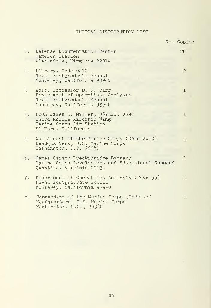
INITIAL DISTRIBUTION LIST

No. Copies

1. Defense Documentation Center 20Cameron StationAlexandria, Virginia 22314

2. Library, Code 0212 2

Naval Postgraduate SchoolMonterey, California 93940

3. Asst. Professor D. R. Barr 1

Department of Operations AnalysisNaval Postgraduate SchoolMonterey, California 93940

4. LCOL James E. Miller, 067320, USMC 1

Third Marine Aircraft WingMarine Corps Air StationEl Toro, California

5. Commandant of the Marine Corps (Code A03C) 1

Headquarters, U.S. Marine CorpsWashington, D.C. 20380

6. James Carson Breckinridge Library 1

Marine Corps Development and Educational CommandQuantico, Virginia 22134

7. Department of Operations Analysis (Code 55) 1

Naval Postgraduate SchoolMonterey, California 93940

8. Commandant of the Marine Corps (Code AX) 1

Headquarters, U.S. Marine CorpsWashington, D.C, 20380

40

UNCLASSIFIEDSecurity Classification2

DOCUMENT CONTROL DATA -R&D(Security classification of title, body ol abstract and indexing annotation must be entered when the overall report Is classified)

I ORIGINATING ACTIVITY (Corporate author)

Naval Postgraduate SchoolMonterey, California 939^0

la. REPORT SECURITY CLASSIFICATION

Unclassified2b. GROUP

3 REPORT TITLE

A GOODNESS OF FIT TEST FOR BIVARIATE NORMAL DISTRIBUTION

4 descriptive NO T E S (Type of report and, inclusi ve dates)

Master's Thesis; April 19708 AUTHORISI (First name, middle initial, laal name)

James Edward Miller, Lieutenant Colonel, United States Marine Corps

6 REPOR T D A TE

April 1970

la. TOTAL NO. OF PAGES

40

76. NO. OF REFS

78a. CONTRACT OR GRANT NO.

b. PROJEC T NO

9a. ORIGINATOR'S REPORT NUMBER(S)

96. OTHER REPORT NOIS) (Any other numbers that may ba assignedthis report)

10 DISTRIBUTION STATEMENT

This document has been approved for public release and sale;its distribution is unlimited.

II SUPPLEMENTARY NOTES 12. SPONSORING MILITARY ACTIVITY

Naval Postgraduate SchoolMonterey, California 939^0

13. ABSTR AC T

This paper is an investigation of a goodness of fittest for bivariate normal distributions. The test proced-ure is based on random linear functions of bivariatenormal random variables. The test makes use of the maximumKolmogorov D(M) statistic over the linear functions whichare computed. An estimate of the distribution of M isobtained by computer simulation. No attempt is made todetermine the power of the test.

DD """ 1473t NOV 68 I "T # WS/N 0101 -807-681

1

(PAGE 1)UNCLASSIFIED

41 Security ClassificationA-31408

UNCLASSIFIEDSecurity Classification

KEY WORDSROLE W T ROLE AT ROLE W T

GENERATION OF BIVARIATE NORMALRANDOM VARIABLES

GOODNESS OF FIT TEST

BIVARIATE NORMAL DISTRIBUTION

I

DD F ° R:.,1473 back)

a 2

UNCLASSIFIEDSecurity Classification a - 3 i 4 01

ThesisM5873c.l

U:; 8

Mi HerA goodness of fit

test for bivariatenormal distributions.

ThesisM5873c.l

A J v^

MillerA aoodness of f i t

test for bivariatenormal distributions.

thesM5873

A,.?.?.°.

dness of fit test for bivariate nor

3 2768 000 98263 1

DUDLEY KNOX LIBRARY

a goodness of fit test for bivariate normal distributions. ·...

Documents