a global shear velocity model of the upper mantle from...

A global shear velocity model of the upper mantlefrom fundamental and higher Rayleighmode measurements

Eric Debayle1 and Yanick Ricard1

Received 6 March 2012; revised 12 September 2012; accepted 12 September 2012; published 24 October 2012.

[1] We present DR2012, a global SV-wave tomographic model of the upper mantle.We use an extension of the automated waveform inversion approach of Debayle (1999)which improves our mapping of the transition zone with extraction of fundamental andhigher-mode information. The new approach is fully automated and has been successfullyused to match approximately 375,000 Rayleigh waveforms. For each seismogram,we obtain a path average shear velocity and quality factor model, and a set of fundamentaland higher-mode dispersion and attenuation curves. We incorporate the resulting set ofpath average shear velocity models into a tomographic inversion. In the uppermost 200 kmof the mantle, SV wave heterogeneities correlate with surface tectonics. The high velocitysignature of cratons is slightly shallower (≈200 km) than in other seismic models.Thicker continental roots are not required by our data, but can be produced by imposinga priori a smoother model in the vertical direction. Regions deeper than 200 km showno velocity contrasts larger than �1% at large scale, except for high velocity slabs withinthe transition zone. Comparisons with other seismic models show that current surface wavedatasets allow to build consistent models up to degrees 40 in the upper 200 km of themantle. The agreement is poorer in the transition zone and confined to low harmonicdegrees (≤10).Citation: Debayle, E., and Y. Ricard (2012), A global shear velocity model of the upper mantle from fundamental and higherRayleigh mode measurements, J. Geophys. Res., 117, B10308, doi:10.1029/2012JB009288.

1. Introduction

[2] The dramatic increase in the number of seismic sta-tions in the last 25 years has stimulated the development ofautomated approaches for global imaging of Earth’s uppermantle [e.g., Trampert and Woodhouse, 1995; van Heijst andWoodhouse, 1997; Debayle, 1999; Beucler et al., 2003;Lebedev et al., 2005; Yoshizawa and Ekstrom, 2010]. Theseapproaches are based on the analysis of surface wave data-sets [Trampert and Woodhouse, 1995] sometimes includinghigher-modes [Debayle et al., 2005; Beucler and Montagner,2006; van Heijst and Woodhouse, 1999].[3] Most resulting S-wave models have been built using

ray theory. At first glance, these shear-wave models are veryconsistent in the upper 200 km of the mantle, where they allhave a very strong correlation with surface tectonics. How-ever, a further comparison shows that these seismic models

differ, even for wavelengths which exceed 1500 km, wherethe most conservative estimate confirms that ray theory isvalid [Spetzler and Snieder, 2001]. As an illustration weshow in Figure 1 a comparison between two recent SV-wavemodels at 100 km depth, S40RTS by Ritsema et al. [2011]and DKP2005 by Debayle et al. [2005]. Both models arebased on ray theory and use Rayleigh waves analyzed in theperiod range 50–200 s. Significant differences are presentat wavelengths greater than 1500 km, for example beneathTibet, Europe, Australia or in oceanic areas. Such differ-ences cannot be attributed to the theory, which is the samefor both models. They have to be related to the way datahave been extracted from the seismograms, or to the strat-egy and practical details of the inversion. For example,DKP2005 first constructs 1D radial models for all the raysbefore combining them in a 3D model, while S40RTS startsfrom 2D phase dispersion maps, before a depth dependentinversion. The parameterization, the a priori model, themethod of regularization and the data weighting, are alsospecific to each tomographic model.[4] This issue is important, because recent developments

aim at improving the resolution of tomographic models usingmore sophisticated theories. In places where seismic modelsshow differences over wavelengths at which ray theory isvalid, there is few hopes that smaller scale features inferredfrom a more sophisticated theory will provide valuable newinformation.

1Laboratoire de Géologie de Lyon: Terre, Planètes et Environnement,CNRS, Université de Lyon 1, Ecole Normale Supérieure de Lyon,Villeurbanne, France.

Corresponding author: E. Debayle, Laboratoire de Géologie de Lyon:Terre, Planètes et Environnement, CNRS, Université de Lyon 1, EcoleNormale Supérieure de Lyon, 2 rue Raphaël Dubois, Bâtiment Géode,FR-69622 Villeurbanne CEDEX, France. ([email protected])

©2012. American Geophysical Union. All Rights Reserved.0148-0227/12/2012JB009288

JOURNAL OF GEOPHYSICAL RESEARCH, VOL. 117, B10308, doi:10.1029/2012JB009288, 2012

B10308 1 of 24

[5] We believe therefore crucial to improve the way infor-mation is extracted from the data. One may hope that ifseismologists agree on the robust dataset to be used in theinverse problem, a major cause of differences between cur-rent seismic models would disappear. This would provide astrong basis for future finite-frequency inversions.[6] There are several ways to extract information from a

surface wave seismogram. The most common approach isto derive path average phase or group velocity curves forthe fundamental mode of surface waves [e.g., Trampert andWoodhouse, 1995; Ekstrom et al., 1997; Ritzwoller et al.,2002; Nettles and Dziewonski, 2008]. In the period rangecommonly used for global surface wave analysis (50–300 s),fundamental modes primarily constrain the upper 300 kmof the mantle. Higher-mode information is sensitive to thedeeper structure and can provide valuable information onthe transition zone which is poorly sampled by body waves.However modeling higher-modes requires sophisticatedapproaches, because they propagate with similar group veloc-ities and are thus difficult to separate in the time domain.[7] Two approaches are commonly used to extract higher-

mode information. The first involves clusters of stations[Nolet, 1975; Cara, 1979] or of events located at differentdepths but within a small epicentral area [Stutzmann andMontagner, 1993; Beucler et al., 2003]. The second usessingle seismograms [Cara and Lévêque, 1987; Nolet, 1990;van Heijst and Woodhouse, 1997; Yoshizawa and Kennett,

2002; Visser et al., 2007] and is better suited to achievedense ray coverages in tomographic studies.[8] The mode branch stripping technique of van Heijst and

Woodhouse [1997] was designed for long paths (>50�), typi-cal of global tomography, for which higher-mode branchescan be separated because their dispersion curves are suffi-ciently different.[9] Waveform inversions [Cara and Lévêque, 1987; Nolet,

1990; Yoshizawa and Kennett, 2002] have been designedfor short paths (<50�) typical of regional tomography. Theidea is to find a path average 1D model which explainsthe waveform of a seismogram and takes into account allthe information present in the different modes which inter-fere in this waveform. The resulting 1D-model can be seeneither as a specific path-average structure [Cara and Lévêque,1987; Nolet, 1990], or as a summary of the fundamentaland higher-mode dispersion curves [Yoshizawa and Kennett,2002; Visser et al., 2008].[10] Yoshizawa and Kennett [2002] and Visser et al. [2008]

use non-linear waveform fitting with the neighborhood algo-rithm of Sambridge [1999] to obtain path specific 1D modelswhich are then used to estimate multimode dispersion curves.Nolet [1990] uses waveform fitting of suitably filtered seis-mograms, starting from long period, where the seismogramis less sensitive to the strongest heterogeneities of the upper-most mantle, and shifting progressively to shorter periods.Because of the strong non linearity of the waveform inver-sion, this approach requires an accurate starting model inorder to avoid solutions corresponding to secondary minimaof the cost function.[11] The approach of Cara and Lévêque [1987] is based

on the definition of secondary observables, built up from theseismograms, having only a slightly non-linear dependenceupon the model parameters. This minimizes the dependenceon the starting model. Debayle [1999] extends this approachwith an automated procedure able to match the waveformsof large volumes of individual records, starting with syntheticseismograms computed with a single upper mantle model.This automated approach has been used in many regional[e.g.,Debayle et al., 2001; Sieminski et al., 2003; Pilidou et al.,2004;Heintz et al., 2005;Maggi et al., 2006a, 2006b; Priestleyet al., 2008] or global [Debayle et al., 2005] studies.[12] A first goal of this paper is to extend Debayle’s [1999]

approach in order to improve the extraction of informa-tion, especially higher-modes, from a surface wave seismo-gram. We summarize the original Cara and Lévêque [1987]approach in section 2 and the new automated scheme insection 3. The new method increases the computation timerequired to model a single waveform by a factor of 10, but aBeowulf computer makes it possible to process hundreds ofthousands of seismograms in a few weeks.[13] A second goal is to present DR2012, our new global

3D SV-model of the upper mantle. In section 4, we apply thenew approach to a global dataset of fundamental and higher-mode Rayleigh waves that includes 374,897 waveforms. Foreach waveform we derive a path average 1D S-velocity andquality factor model, and a set of fundamental and higher-mode dispersion and attenuation curves compatible with therecord. We then combine the set of 1D S-velocity models ina tomographic inversion to built DR2012. In section 5 wefirst show that the new approach extracts more information

Figure 1. SV-wave perturbations relative to PREM at100 km depth in two tomographic models: (top) DKP2005by Debayle et al. [2005] and (bottom) S40RTS by Ritsemaet al. [2011]. The color scale is in per cent.

DEBAYLE AND RICARD: GLOBAL SHEAR WAVE VELOCITY DISTRIBUTION B10308B10308

2 of 24

compared with Debayle [1999], and improves our mappingof heterogeneities, especially within the transition zone.Then we compare DR2012 with other seismic models.

2. Waveform Inversion

2.1. Synthetic Seismograms

[14] In Cara and Lévêque [1987], the surface wave isrepresented by a finite sum of pure-mode synthetics com-puted for a laterally homogeneous medium. The expressionof a pure-mode synthetic sp(t) is given by:

sp tð Þ ¼ g xð ÞZ

I wð ÞSp wð Þe�ap wð Þxei wt�kp wð Þx½ �dw ð1Þ

where p is the mode rank, x the epicentral distance, g(x) thegeometric expansion, w the circular frequency, I(w) the instru-mental response, Sp(w) the complex source excitation, ap(w)the apparent attenuation factor and kp(w) the wavenumberfunction.[15] The source excitation Sp(w) is computed using a spe-

cific crustal and upper mantle model taken at the epicenterlocation. This 1D model is obtained by extracting density,seismic velocities and attenuation from 3SMAC [Nataf andRicard, 1995] beneath the epicenter. Sp(w) is then com-puted following Cara [1979], using the global CMT solution[Dziewonski et al., 1981; Ekstrom et al., 2012] issued at theLamont-Doherty Earth Observatory of Columbia University.

[16] The attenuation ap(w) and wavenumber kp(w) arecomputed following Takeuchi and Saito [1972] for a 1Dmodel adapted for each ray. This model includes a path aver-aged crust structure estimated from 3SMAC [Nataf andRicard, 1995]. The upper mantle part is radially anisotropicand very close to PREM at a reference period of 100 s[Dziewonski and Anderson, 1981] for density and elasticparameters, although the 220 km discontinuity has beensmoothed out (see Figure 2). The attenuating layer locatedat 80 km depth in PREM represents a strong a priori choicewhich is not adapted to continental paths for which the atten-uating layer is less pronounced or located deeper. We usetherefore a uniform 1D quality factor Qb(z) of 200 as a start-ing upper mantle model (see Figure 2g). The wavenumberis corrected from physical dispersion using Kanamori andAnderson [1977] assuming a reference period of 100 s.[17] This careful choice of the a priori information for the

starting model in the source region and the average crustalstructure along each epicenter-station path allows us to invertfor the path-average upper mantle structure only, assumingthe crustal structure and the source excitation are known.We tested the impact of the crustal model to the finaltomographic maps in some of our previous papers [Debayleand Kennett, 2000; Pilidou et al., 2004; Priestley et al.,2008]. Crustal corrections done with 3SMAC or CRUST2[Bassin et al., 2000] have no effect under oceans wherethe average crust is much thinner (�7 km) than the depthof maximum sensibility of Rayleigh waves (≥70 km for

Figure 2. Our 1D starting model (blue) superimposed to PREM (red) at a reference period of 100 s.For the inverted parameters (Vs and the shear attenuation) we also plot in green the 1D models obtainedafter averaging the 374,897 inverted profiles. For Vs, this inverted model is very close to the 1D startingmodel in blue.


3 of 24

periods larger than 50 s). Even on continents where the crustis thick, the effects of crustal corrections, whether using3SMAC or CRUST2, are undistinguishable at depths largerthan 100 km depth and minor before [Debayle and Kennett,2000; Pilidou et al., 2004]. However, in order to avoid anypossible contamination of our model by the crustal structure,we will only show tomographic maps for depths greater thanor equal to 100 km.[18] At periods greater than 50 s, a combination of 6 pure-

mode synthetics sp(t) is sufficient for an accurate descriptionof the waveform in the group velocity window associatedwith surface waves. The complete synthetic seismogram s(t)is thus obtained by summing pure-mode synthetics sp(t) forthe fundamental mode and the first five overtones:

s tð Þ ¼X6p¼1

sp tð Þ: ð2Þ

2.2. Secondary Observables

[19] The secondary observables introduced by Cara andLévêque [1987] are the starting data for the waveforminversion. They are extracted from the observed and syn-thetic seismograms, s(t) and s (t) by cross-correlation withsynthetic seismograms for individual modes sp(t) computedfor a reference model. The resulting cross-correlograms arethen band-pass filtered around different frequencies. Thecombination of band-pass filtering and cross-correlation canbe represented as:

gp wq; t� � ¼ h wq; t

� �∗ s tð Þ∗ šp �tð Þ; ð3Þ

for an observed cross-correlogram, and:

gp wq; t� � ¼ h wq; t

� �∗ s tð Þ ∗ šp �tð Þ; ð4Þ

for a synthetic cross-correlogram. Here * denotes a convo-lution, h(wq, t) is the impulse response of a band-pass filtercentered on the circular frequency wq, and šp denotes thecomplex conjugate of sp. The actual secondary observablesused by Cara and Lévêque [1987] are defined by samplingthree values taken at different time lags on the observedenvelope of the modal cross-correlograms gp(wq, t), with avisual inspection of the envelope. One value is taken at theappropriate maximum of the envelope and two others oneither side of this position. The inversion minimizes thedifference between these observables and those computedfor a complete synthetic seismogram s(t). The instantaneousphase of the cross-correlogram, taken at the time where theenvelope reaches its maximum is generally also included toadjust the waveform fit.

2.3. 1D Model Inversion

[20] A 1D model is then derived to explain each seis-mogram. Following Debayle [1999], this inverted model mincludes the shear wave velocity bv(z), the attenuation param-eterized by log(Qb(z)) and the scalar moment through log(M0).The inversion of log(Qb(z)) accounts for frequency-dependentamplitude differences between the synthetic and recordedwaveforms. As waveform modeling means both phase andamplitude modeling, the inverted bv(z) profiles might bebiased if attenuation is not inverted for and if the startingattenuation model is not accurate enough.

[21] We could have used some a priori information tocorrelate changes in shear velocity to those in compressionalvelocity, density and radial anisotropy. However, our expe-rience in agreement with previous studies [e.g., Nishimuraand Forsyth, 1989], shows that this kind of a priori couplingdoes not change the results for the best resolved parametersbv(z) and log(Qb(z)), while the others are essentially con-strained by the a priori information. Therefore, the radialanisotropy, density and Vp velocity profiles remain fixed totheir initial values in the inversion.[22] In this paper, we do not discuss in details the inverted

log(Qb(z)) model. Unambiguous interpretation of log(Qb(z))requires a good control of the source parameters (there is astrong trade-off between them [Lévêque et al., 1991]) andcorrections of focusing-defocusing effects. However, we showin Figure 2 the 1D bv(z) and log(Qb(z)) models obtainedafter averaging our whole dataset. The average velocity model(Figure 2c, green curve), is very close to the starting model.The average attenuation model remains globally less atten-uating than PREM (Figure 2g, green curve). It has an atten-uating layer located between 100 and 200 km, similar toPREM. This attenuating layer is not present in the startingmodel, and is therefore required by our data.[23] The secondary observables depend upon the model

parameters through weakly non-linear relations [Cara andLévêque, 1987] which are inverted using few iterations[Lévêque et al., 1991; Tarantola and Valette, 1982]. Theinverted model mkþ1 at iteration k + 1 is given by:

mkþ1 ¼ m0 þ Cm0Gtk GkCm0G

tk þ Cd0

� ��1

d� d mkð Þ þGk mk �m0ð Þ½ � ð5Þ

In equation (5), m0 is the a priori model, t denotes the trans-pose, the matrix Gk contains the partial derivatives of thesecondary observables with respect to the model parameters,calculated following Cara and Lévêque [1987], Cm0 and Cd0

are the a priori covariance matrices for model and data.[24] The matrix Cd0 is assumed to be diagonal. Its diago-

nal terms are the variances of the secondary observables anddescribe the errors made on the data measurements. We usea standard deviation of 10% of the value of the envelope dataand 5% of 2p radians for the phase data.[25] The a priori covariance function Cm0 is composed of

three sub-matrices expressing separately the covariances onvelocity, attenuation and seismic moment. No a priori cross-covariances exist between these sub-matrices. For velocityand attenuation, the covariance function between two depthsz1 and z2 is defined after Lévêque et al. [1991]:

Cm0 z1; z2ð Þ ¼ s1s2 exp� z1 � z2ð Þ2

2L2

!: ð6Þ

The standard deviation si controls the amplitude of a com-ponent of the model perturbation allowed at a given depth zi.We use constant values of 0.05 km s�1 and 0.25 at all depthsfor those of bv(z) and log(Qb(z)). The correlation length Lcontrols the vertical smoothness of the model and we useL = 50 km. A very large standard deviation value of 0.5 forlog(M0) accounts for amplitude differences between syntheticand actual waveforms. There is a clear trade off betweenseismic moment and attenuation. To reduce suspicion on theinverted log(Qb(z)) models, we reject the paths for which


4 of 24

Figure 3. Flow-chart of the automated scheme. Nper is defined in section 3, Nsl and cmaxd are defined in

Appendix A.


5 of 24

the amplitude of the initial synthetic seismogram differs bya factor greater than 10 from the actual waveform.[26] Tarantola and Valette [1982] show that when the non-

linearity is weak, the a posteriori covariance Cm and reso-lution R matrices can be approximated by the formulaeobtained in the linear case:

Cm ¼ Cm0 � Cm0Gt GCm0G

t þ Cd0

� ��1GCm0; ð7Þ

and

R ¼ Cm0Gt GCm0G

t þ Cd0

� ��1G; ð8Þ

where the partial derivatives of G are computed at the finaliteration. We use equation (7) to estimate the a posteriorivariance on the inverted parameters. From equation (8), wecompute the trace of R which corresponds to the number ofindependent pieces of information which are extracted fromthe data.

3. New Automated Scheme

[27] A first automation of the Cara and Lévêque [1987]approach was proposed by Debayle [1999]. The idea wasto mimic the choices of a manual user: selection of a suitableperiod range of inversion for each waveform, decompositionof the waveform inversion into long and short period parts,selection of secondary observables on the envelope of themodal cross-correlogram functions gp(wq, t).[28] Here, we revisit the automation and further divide

the waveform modeling into a larger number of elementarysteps. Such a division gives more flexibility to the code,allowing a better selection of the robust information anda better higher-mode extraction. As in Debayle [1999], theautomated code can be divided into a pre-processing stepand a waveform inversion step which includes the automaticselection of the secondary observables.

3.1. Pre-processing

[29] During this step, we prepare the data for the wave-form inversion and we choose the central frequencies wq ofthe band pass filter gp(wq, t). We first check for each recordthat all the necessary information (instrument response, globalCMT determination [Dziewonski et al., 1981; Ekstrom et al.,2012]) is available. Then, we set the header records to thecentroid origin time and location provided by the Lamont-Doherty Earth Observatory of Columbia University and weselect a group velocity window (between 2.5 and 7 km s�1)around the surface wave part of the seismogram.[30] For each record, we use a maximum of five band-pass

filters, with the following sequence of central periods: 250,165, 110, 75 and 50 s. These filters are described in details inAppendix A.[31] Starting from the band pass filter at 250 s, we compare

the amplitude of the envelope of the signal As (part of therecord arriving with a group velocity larger than 3 km s�1) tothe amplitude of the envelope of the noise An (part of therecord arriving with a group velocity smaller than 3 km s�1).Only when As/An is larger than a threshold value (3 in thisstudy), is the data kept at this period. Then, we repeat theprocess to the next period, 165 s, until the last period of 50 s.All the records for which the signal to noise criterion As/An > 3

is not reached at least at 50 and 75 s are rejected. The use offiltered cross-correlogram in the period range 50–75 s issufficient to constrain the SV-wave velocity up to a depthgreater than 250 km, even when only the fundamental modeis taken into account in the inversion [Lévêque et al., 1991].At the end of the preprocessing step, an appropriate numberNper of band-pass filters has been selected for each record,with Nper ranging between 2 and 5. For the best records,Nper = 5 corresponding to robust records around the periods250-165-110-75-50 s. The lowest quality records have Nper

= 2 at periods 75–50 s.

3.2. Step-by-Step Inversion

[32] For each path, the recorded waveform is fitted thougha complex series of steps, each step requiring a new level ofaccuracy in the quality of the fit.[33] First, we match the envelopes of the cross-

correlograms. For a seismogram for which Nper band-passfilters have been selected, the inversion starts with the longestperiod. Once the filtered modal envelope has been matched atsome period, the automated code adds the next shorterperiod. In the best cases, the fit of the cross-correlogramsenvelopes are therefore refined Nper = 5 times (at 250 s only,then simultaneously at 250 s and 165 s, until the five periods250-165-110-75-50 s are included). In the cases Nper = 2,only two refinements are made (75 s, then 75 s and 50 s).[34] Second, for the same record, we also match the instan-

taneous phase of the filtered cross-correlograms. Here againwe proceed period by period, starting from the longest periodand adding successively the details of the shorter periods. Theinversion of the envelope for the whole frequency rangeexplains the group velocity of the different mode branchesof the seismogram. Adding the instantaneous phase furtherincreases the precision of the fit. The strategy of incrementalfit from long to short periods, avoids phase skips of 2p.This approach is close to that followed by van Heijst andWoodhouse [1997] but the inversion is not separated modeby mode. At a given frequency, all the modes which con-tribute more than 1% of the total energy of the initial syntheticseismogram are considered in the inversion.[35] The new scheme allows us to analyze the funda-

mental and up to 5 overtones in the period range 50–250 s.Figure 3 provides a flow-chart of the new scheme and acomplete description of its implementation is provided inAppendix A.

4. Tomographic Inversion

4.1. Dataset

[36] We have applied our automated scheme to a globaldataset of 960,364 Rayleigh wave seismograms recordedbetween 1977 and 2009. Most seismograms have beenrecorded at permanent stations of the Global SeismographicNetwork (GSN) and the International Federation of DigitalSeismographic Networks (FDSN). We also use data fromFrench temporary experiments in the Horn of Africa, FrenchPolynesia [Barruol et al., 2002] and Aegean-Anatolia regionafter the SIMBAAD experiment [Salaün et al., 2012], fromPASSCAL experiments in Africa, Tibet and New-Zealandand from the SKIPPY temporary deployment in Australia.Finally, we included data of USArray Transportable Array


6 of 24

and Reference Network Stations. The distribution of sta-tions used in this study is shown in Figure 4.[37] The automated waveform inversion is distributed over

the nodes of a Beowulf cluster. Using a 45 nodes Beowulfcluster, each node with two quad-core processors, the wholedataset is processed in about 10 days. About 39% of therecords pass successfully all stages of the waveform inver-sion, corresponding to 374,897 accepted waveforms througha total of �20 million secondary observables fitted.

4.2. Regionalization

[38] The waveform inversion yields about 375,000 pathaverage bv(z) and log(Qb(z)) models. It also yields a set ofmultimode dispersion and attenuation curves compatiblewith each surface wave record. These multimode dispersioncurves provide a unique global database for future finite fre-quency inversions. In this paper, we focus on the tomographicinversion of the velocity and we leave the inversion ofattenuation to a future paper (notice that this effective qualityfactor includes effects related to the focusing-defocusing ofthe wave energy by the seismic velocity anomalies, in addi-tion to real dissipation).[39] The tomographic inversion is based on the continu-

ous regionalization formalism of Montagner [1986], whichis derived from the approach developed by Tarantola andValette [1982]. A smooth model is obtained by imposingcorrelations between neighboring points using a Gaussiana priori covariance function on the form of equation (6),but where L is now a horizontal correlation length whichcontrols the lateral degree of smoothing of the invertedmodel, while the a priori model standard deviation s con-trols its amplitude.[40] Montagner [1986] inverted path average group or

phase velocity curves for lateral variations of velocity andazimuthal anisotropy. However, his approach can also be

used to retrieve the local distribution of shear velocity andazimuthal anisotropy from a set of path average bv(z) models[Lévêque et al., 1998]. In this paper, we use a tomographicscheme for massive surface wave inversion developed byDebayle and Sambridge [2004] which incorporates varioussophisticated geometrical algorithms which dramaticallyincrease the computational efficiency and render possible theinversion of massive datasets.[41] Our tomographic scheme is based on the “great circle

ray theory” assumption that surface waves propagate alongthe source-station great circles, and that they are only sen-sitive to the structure along a zero-width ray. Although moresophisticated finite frequency theories exist [Marqueringet al., 1996; Yoshizawa and Kennett, 2002; Spetzler et al.,2002], several authors [e.g., Sieminski et al., 2004; Trampertand Spetzler, 2006] have shown that finite-frequency effectscan be accounted for by a physically-based regularizationof the inversion. Sieminski et al. [2004] performed a seriesof synthetic tests, comparing Debayle and Sambridge [2004]tomographic scheme with a finite frequency inversion basedon linearized scattering theory [Spetzler et al., 2002]. Theyshow that results obtained using Debayle and Sambridge[2004] scheme are consistent with those of finite-frequencyinversion, provided the path coverage is dense enough. Forthese reasons, we believe that a finite frequency approachwould be computationally too expensive and would not allowsignificant progress compared with our tomographic scheme,which incorporates a sophisticated a priori information inthe inverse problem.[42] Following Lévêque et al. [1998], we apply the Debayle

and Sambridge [2004] code directly to the bv(z) path aver-age models and we invert for the local distribution of shearvelocity including or not azimuthal anisotropy. We use ahorizontal correlation length of L = 400 km, and a standarddeviation s = 0.05 km s�1 for the isotropic component of

Figure 4. Location of stations (stars) used in this study.


7 of 24

the shear wave velocity. We have undertaken inversionswith or without azimuthal anisotropy. When inverting forazimuthal anisotropy, we use an a priori standard deviationof 0.005 km s�1 for the anisotropic components of the shearwave velocity. Increasing L leads to smoother tomographicimages with higher amplitude anomalies, but the overallpattern of anomalies remains unchanged. For comparisonwith models expressed in spherical harmonics, our modeluses spherical harmonics up to the degree l ≈ (2pR)/L ≈ 45,where R is Earth’s radius. In this paper we only discuss theisotropic part of the model and leave the anisotropic part toa future paper.

4.3. Path Clustering

[43] We follow Debayle and Sambridge [2004] to com-bine the selected bv(z) models in the tomographic inver-sion, as described in section 4.2. At this stage, we use thea posteriori error on bv(z) models to weight the data. Thea posteriori covariance matrix is related to the a prioricovariance matrix by:

Cm ¼ I� Rð ÞCm0 ð9Þ

Therefore, at a given depth, the a posteriori error is largeand close to the a priori error when the actual waveformcontains little information on the bv(z) structure (i.e. whenR is close to zero), while it decreases when R approachesidentity. For this reason, we keep only the bv(z) modelsfor which the a posteriori error is smaller than 80% of thea priori error at a given depth. By this way, only wellresolved path average bv(z) model are used in the tomo-graphic inversion at all depths.[44] To decrease the computing time and memory require-

ment, we cluster at each depth the selected path-average bv(z)models associated with close epicenters recorded at a givenstation. We use a cluster radius of 200 km (i.e. smaller thanthe correlation length) and consider that the waves of agiven cluster follow the same path and see the same averageEarth structure between the epicenters and the station. Ateach depth, we select from each cluster the “best resolved”bv(z) model. The best resolved bv(z) model has the largesttrace of R.[45] After this clustering, our �375,000 bv(z) models

reduce to �125,000 clusters corresponding to “independent”well-resolved paths. At depths greater than 200 km, thenumber of independent paths decreases because onlyintermediate-to-deep events located in subduction zonesprovide well excited higher-modes and well resolved shearvelocities. At 400 km depth, the number of independentpaths is close to �30,000. It exceeds 20,000 paths downto 575 km, while 11,007 paths still remain at 700 km depth.We show in section 4.4 that this provides a global coverageof the Earth within the upper mantle and transition zone.[46] Note that our data selection strategy differs from pre-

vious applications of the Debayle [1999] algorithm byDebayle et al. [2005] andMaggi et al. [2006a]. These authorsuse the a posteriori error on each individual bv(z) model asa guide to discard data which provide little resolution in agiven depth range. Then, they cluster the remaining dataand extract from each cluster the mean shear wave velocity

�bv(z) and its standard deviation �s(z). They use �bv(z) and �s(z)along the average paths for the tomographic inversion.[47] Our choice of extracting the best resolved bv(z) model

of each cluster preserves the number of independent paths butavoids loss of resolution through averaging with less resolvedmodels. Furthermore, it allows us to use the a posteriorierror issued from the waveform modeling in the tomo-graphic inversion. By this way, we carry in the tomographicinversion the information related to the depth sensitivity ofthe actual dataset, an information which is lost when using�bv(z) and its standard deviation.

4.4. Data Coverage and Errors

[48] Figure 5 shows the number of rays crossing a 400 �400 km surface area at various depths within the uppermantle. These maps are typical of global seismology withstrong bias towards the continents of the northern hemisphere.The transition from fundamental to higher mode coverageis observed between 200 and 450 km (Figure 5). However,even in the less covered areas of the transition zone, Figure 5shows that our seismic model includes higher-mode con-straints from 10 to 100 different paths in each 400 � 400 kmsurface area. Therefore, our higher-mode dataset providesglobal coverage of the transition zone with a large numberof redundant data.[49] At this stage, it is worth noting that errors in the

source parameters may bias the path-average shear velocityestimation for some of the 1D models. However, the pathsfor which this bias might be strong are rejected by applyingthe selection criteria (see section A2). For the other paths,these effects have no reason to be coherent since they arerelated to earthquakes with different focal mechanisms ordifferent focal depths. Therefore, they should average out inour tomographic inversion which involves a large number ofpaths with different azimuths.

4.5. Tomographic Maps

[50] The SV-velocity distribution at different depths for anisotropic inversion is depicted in Figure 6. Figure 7 showsthe equivalent result for an inversion including azimuthalanisotropy. Comparison of Figures 6 and 7 proves thatextracting azimuthal anisotropy does not alter significantlythe isotropic component. The main difference is a slightlylarger amplitude of SV-wave perturbation in the isotropicinversion by up to 2% at 150 km depth, reducing to lessthan 0.6% at depths greater than 200 km. At 150 km depth,the most noticeable differences occur in the Pacific, in agree-ment with Ekstrom [2011]. Our preferred SV-velocity modelis the isotropic component of the anisotropic inversion asshown in Figure 7, because it is corrected for the small biasdue to azimuthal anisotropy. In the next figures of thispaper, we will always discuss and show the isotropic part ofan anisotropic model.[51] In the upper 200 km of the mantle, DR2012 (Figure 7)

shows a very close correlation with surface tectonics.Mid oceanic ridges have a strong slow velocity signature in thefirst 100 km depth under all oceans younger than �40 Myrs.This localized slow signature of ridges is rather shallow andvanishes rapidly between 100 and 150 km depths after whichall oceans have a rather homogenous slow velocity.


8 of 24

[52] The map at 150 km depth shows high seismic veloc-ities associated with the thick lithosphere of Archean andProterozoic cratons and low seismic velocities beneathoceanic regions and most Phanerozoic continents. In theseregions, low seismic velocities correspond to the low veloc-ity layer associated with the asthenosphere. Exceptions areobserved in the Andes where active subduction is present,and beneath Tibet, where continental collision of Asia andsouthern Eurasia favors underthrusting by a high velocityIndian mantle [Priestley et al., 2006]. The signature of con-tinental roots fades away around 200 km depth suggestinga seismic lithosphere on the low end of what has beenestimated for the thermal cratonic lithosphere (thicknessesof 200–300 km are usually proposed [e.g., Jaupart andMareschal, 1999]), but in agreement with what is deducedfrom gravity models [Lestunff and Ricard, 1995].[53] Between 250 km depth and down to the top of the

transition zone, the correlation with surface tectonics is lost

(Figure 7). However, within the transition zone, a pattern ofhigh seismic velocities associated with subductions aroundIndonesia and the Pacific, and in the Mediterranean region isretrieved. This suggests some “ponding” of the slabs withinthe transition zone, producing a broad scale high velocitysignature picked-up by long period surface waves.[54] Figure 8 depicts the root mean square (RMS) of

velocity perturbations as a function of depth. The strongestRMS perturbations are between 100 and 150 km depths,where DR2012 correlates well with surface tectonics. Theselarge RMS perturbations are due to the strong high velocitysignature of cratons contrasting the strong low velocity sig-nature of oceanic and Phanerozoic asthenosphere. The RMSof velocity perturbations decreases by a factor of 3.5 between150 and 250 km and stabilizes at greater depths. This abruptdecrease is also observed in other seismic models [Kustowskiet al., 2008]. It likely marks the base of the continentallithosphere.

Figure 5. Ray density maps at different depths. Black and white scale indicates the number of rays nor-malized over a 4 by 4 degrees area.


9 of 24

[55] In Figure 9 we plot the age-dependent average cross-section of DR2012. The oceanic part of Figure 9 was createdby taking sliding window averages of our SV-velocity dis-tribution along the Müller et al. [2008] isochrons. SV-velocity contours deepen progressively with age and followapproximately the trend predicted by the square root of agecooling model [Turcotte and Schubert, 2002]. This obser-vation confirms with an up-to-date global dataset a resultsuggested by most previous surface wave studies of litho-spheric cooling [e.g., Forsyth, 1977; Zhang and Tanimoto,1991; Zhang and Lay, 1999; Maggi et al., 2006a]. How-ever, for ages larger than 100 Myrs, some flattening of theisotherms may be seen as predicted by models where a

constant heat flux is provided at depth [Doin and Fleitout,1996; Goutorbe, 2010].[56] The continental part of Figure 9 consists in three aver-

age 1D profiles of SV-velocity, for Phanerozoic, Proterozoicand Archean tectonic provinces. Tectonic provinces aredefined after the 3SMAC model of Nataf and Ricard [1995].These 1D profiles are shown as absolute velocities (Figure 9,right) and as SV-velocity perturbations (Figure 9, left).Continental profiles are only shown at depths greater orequal to 100 km, where the effect of crustal correction isnegligible. Phanerozoic provinces regroup heterogeneousregions including active orogens (e.g. Tibet and the AndeanCordillera) and stable Paleozoic lithosphere. For this reason,

Figure 6. SV velocity distribution at different depths for an isotropic inversion. Perturbations from thereference velocity in percent are displayed by color coding. The velocity varies from �10% to +10% fromthe average value in the uppermost 250 km. At greater depths, shear velocity perturbations are between�3% to +3% to emphasize smaller contrasts.


10 of 24

the 1D Phanerozoic profile is difficult to interpret. On aver-age, Archean lithosphere is faster and slightly thicker thanProterozoic lithosphere. Figure 9 confirms that the seismicsignature of cratons has entirely vanished at 250 km depth.

5. Discussion

5.1. Improvements Due to the New Automated Scheme

[57] In this section, we compare the new scheme withthe automated waveform modeling of Debayle [1999].63,514 waveforms have been matched successfully usingboth approaches. The resolutions matrix R is computedafter each waveform inversion using equation (8). The traceof R gives the number of independent parameters extracted

by each inversion. Table 1 reports the trace of R aver-aged for events belonging to different depth ranges. For alldepth ranges, the new scheme extracts more information.This additional information is due to a wider period range(up to 250 s), the inclusion of 5 higher-modes instead of 4in Debayle [1999], and the selection of more secondaryobservables on each modal envelope. The smallest improve-ment (0.32) is obtained for shallow events (0–50 km) whichconcentrate their energy in the fundamental mode of surfacewaves. For deep events (200–700 km) which have mostof their energy in the higher-modes, 0.63 additional degreeof freedoms are extracted. The largest improvement (0.96)is obtained for intermediate depth events (50–200 km), forwhich both fundamental and higher-modes are well excited.

Figure 7. Same as Figure 6 but for an inversion including azimuthal anisotropy. Comparison withFigure 6 shows that the bias due to the presence of azimuthal anisotropy is small. This SV velocity distri-bution corrected from this small bias, is our new seismic model DR2012.


11 of 24

[58] According to equation (6), two points z1 and z2 distantby L and 2L are a priori correlated with values of 0.60 and0.36 respectively. If we consider, as a rule of thumb, that twodepths distant by 2L are “independent”, extracting one moreindependent parameter means that we constrain one addi-tional layer with an approximate width of 2L. The width ofthis layer would be 100 km for L = 50 km.[59] Figure 10 compares DKP2005 [Debayle et al., 2005]

and DR2012 at 150 and 500 km depth. Both models use thesame vertical (L = 50 km) and horizontal (L = 400 km)smoothings. DKP2005 was built from 100,777 waveformsanalyzed using Debayle’s [1999] approach. This model wasonly published for its shallowest 400 km part and the mapat 500 km has been only produced for the purpose of thepresent study.[60] Figure 10 shows that the new scheme improves map-

ping of the transition zone. At 500 km depths, DR2012 dis-plays high seismic velocities associated with subductions,around the Pacific plate and in Europe. This pattern is ingood agreement with others seismic models (see section 5.2).In contrast, DKP2005 is patchy at 500 km. This proves thatthe new approach better extracts the long wavelength seismicheterogeneities at depth, due to a more efficient selection of

l

Figure 8. RMS of velocity perturbation in % computedwithin DR2012 as a function of depth.

Figure 9. (left) Cross-section with respect to age for oceanic regions and Phanerozoic (labeled Pha.),Proterozoic (labeled Prot.) and Archean (labeled Arch.) continental provinces. Color coding shows pertur-bations in percent from the reference SV velocity profile displayed in black in Figure 9 (right). For oceanicregions, a smoothed image was created by averaging SV velocity along theMüller et al. [2008] isochrons,using a sliding age window of 10 Ma width. The continuous black line indicates the position of the thermalboundary layer for the half-space cooling model as defined in, e.g., Turcotte and Schubert [2002]. (right)Reference (black), Paleozoic (green), Proterozoic (red) and Archean (blue) absolute SV velocity profiles.

Table 1. Average Amount of Independent Information ExtractedWith the New Scheme Against the Debayle [1999] Algorithm

Event’s Depth Range

0–50 km 50–200 km 200–700 km 0–700 km

Number of waveforms 43,868 16,559 3087 63,514Debayle [1999] 4.43 4.93 5.86 4.60New scheme 4.75 5.89 6.49 5.13Improvement 0.32 0.96 0.63 0.53


12 of 24

robust secondary observables. The greater benefit is obtainedfor higher-modes, which often have a lower signal to noiseratio compared to the fundamental mode. At 150 km depth,DKP2005 and DR2012 are very consistent although DR2012has a slightly larger amplitude. Here both approaches extractvery well the fundamental mode of surface waves. However,some new features in DR2012 show a better agreement withsurface tectonics (e.g. the slow velocities beneath Hawaii[Wolfe et al., 2011] or the broad region of slow velocitiesbeneath the South Pacific [Tanaka et al., 2009]).[61] We have performed various tests indicating a system-

atic improvement of the resolution of DR2012 with respect toDKP2005 due to both an increase of the number of analyzedseismic paths by a factor 3.5 and a more accurate waveformmodeling. We already published synthetic experiments forsubsets of our data set for regions including Horn of Africa[Debayle et al., 2001], Antarctica [Sieminski et al., 2003],North Atlantic and surrounding regions [Pilidou et al., 2005],Australia [Debayle et al., 2005], Asia [Priestley et al., 2006]and Africa [Priestley et al., 2008]. These tests confirm thatwe are able to isolate upper mantle seismic velocity anomalieslocated at depths larger than 250 km. Rather than repeatinghere these tedious synthetics, we find it more interesting tocompare DR2012 with other seismic models obtained usingdifferent modeling approaches and different datasets. Weshow in the next section that the pattern of seismic hetero-geneities in DR2012 is consistent with other S-wave modelsup to degree 40 within the uppermost 200 km of the mantleand up to degree 10 within the transition zone.

5.2. Correlation With Other Seismic Models

[62] We compute correlations between DR2012 and threeother seismic models: S40RTS by Ritsema et al. [2011],

S362ANI by Kustowski et al. [2008] and HMSL by Houseret al. [2008].[63] S40RTS is an isotropic S-wave model based on three

data sets: fundamental and higher mode Rayleigh waves,spheroidal normal modes and teleseismic travel times oflong period body waves. Teleseismic travel times are mostlySH-type waves measured on the transverse components(except for SKS phases). These waves, which generally havesteep incidence in the upper mantle, are essentially affectedby the lower mantle structure. The upper mantle is largelyconstrained by Rayleigh wave fundamental and higher modesand spheroidal normal modes, which are sensitive to SV.However, some SH-type body wave phases like SS, SSSand SSSS have a significant portion of their paths in theupper mantle. In a transversely isotropic medium with avertical axis of symmetry like PREM, SH-polarized wavestraveling nearly vertically experience no splitting and aresensitive to SV. However, for typical S-wave wavelengthsof few tens of kilometers, the preferred orientation of aniso-tropic minerals generally produces azimuthal anisotropywhich is better represented by a transversely isotropic mediumwith an horizontal symmetry axis. Although this azimuthalanisotropy is averaged out in a global model like PREM,most SH-type waves traveling nearly vertically in the uppermantle may provide a different information than Rayleighwaves and spheroidal modes. We assume that the differencein parameter sensibilities of these two data sets was accoun-ted for in S40RTS and we consider S40RTS as essentially anSV model in the upper mantle.[64] S362ANI includes surface wave phase anomalies,

long period waveforms and body wave travel times. Theupper mantle part of S362ANI is primarily constrained bysurface waves and their higher-modes. Higher-modes are

Figure 10. SV-wave velocity distribution at (top) 150 km and (bottom) 500 km depth in DKP2005 byDebayle et al. [2005] compared with maps at the same depths in DR2012. SV-wave perturbations arein per cent relative to PREM.


13 of 24

included in S362ANI through the inversion of long periodmantle (>125 s) and body (>50 s) waveforms. S362ANIincludes measurements from transverse, longitudinal andradial components and allows for the presence of radialanisotropy in the upper 400 km of the mantle. We compareour SV model with the SV-wave part of S362ANI.[65] HMSL is an isotropic S and P velocity model based

on surface waves, long period body wave travel times anddifferential body wave travel times. The upper mantle S-wavevelocity structure of HMSL is mostly constrained by Rayleighand Love phase velocities with minor contribution from bodywaves. However, HMSL does not incorporate radial anisot-ropy, a difference with other models, which are either based onthe analysis of Rayleigh waves only (S40RTS and DR2012),or incorporate radial anisotropy to account for the Love-Rayleigh discrepancy (S362ANI). This may explain somedifferences with other models at the top of the upper mantle,although the use of longer period surface waves (66–250 s) inHMSL mitigates its sensitivity to shallow radial anisotropy.[66] S40RTS, S362ANI and HMSL span the range of pos-

sible data (surface waves fundamental and higher modes, bodywaves, normal modes) which can be used for mapping uppermantle S-wave heterogeneities. They also span a wide rangeof possible model parameterizations (spherical harmonics,splines, blocs, Gaussian correlations) including radial anisot-ropy or not. Other recent seismic models agree well withat least one of these models. For example, SAW642AN byPanning and Romanowicz [2006] is based on a data set com-parable to that of S362ANI. This model correlates well withS362ANI and S40RTS, both for the depth extent of seis-mic heterogeneities and for their long wavelength pattern[Kustowski et al., 2008; Ritsema et al., 2011]. We believethat S40RTS, S362ANI and HMSL summarize our currentknowledge of the large scale S-wave upper mantle structure.

In addition, although these models incorporate datasets whichare not present in DR2012, their upper mantle part is in allcase largely constrained by surface waves.[67] Figure 11 shows the spectra SA

2(l) = ∑m=�ll Al

mAlm* of

these tomographic models at 150 km, 250 km, 500 kmand 610 km (Al

m are the spherical harmonic coefficients atdegree l and azimuthal order m of the tomographic model A,and * denotes the complex conjugate). S362ANI is clearlythe smoothest model. It uses 362 spherical splines, equivalentto a spherical-harmonic degree 18 expansion. For this reason,we do not show spectra or correlations for l > 20 for thismodel. S40RTS is only provided up to degree 40. DR2012and HMSL show a gentle decrease of spectral amplitude.This decrease is more pronounced at high degrees in the caseof DR2012 which does not include body waves. S40RTSseems to favor the even degree anomalies at depth, which islikely due to the contribution of the normal modes in themodel.[68] We use the following relationship to compute the

correlation between two seismic models A and B:

C lð Þ ¼ ∑lm¼�lA

ml B

m∗l

SA lð ÞSB lð Þ ð10Þ

Figure 12 displays the correlations C(l) computed at 150 km,250 km, 500 km and 610 km depths between DR2012 andthe three other seismic models. At 150 km depth, correla-tions are representative of those obtained in the uppermost200 km. At 250 km depth they are representative of thoseobtained between 200 and 400 km, while at 500 and 610 kmdepths, they represent correlations in the upper and lowerparts of the transition zone.[69] At 150 km depth, the correlation between DR2012 and

S362ANI is above the 95% confidence level up to degree 20.

Figure 11. Spectral amplitude as a function of degree for DR2012 (purple line), S40RTS [Ritsema et al.,2011] (blue line), HMSL [Houser et al., 2008] (green line) and S362ANI [Kustowski et al., 2008](red line) at depths of 150, 250, 500 and 610 km.


14 of 24

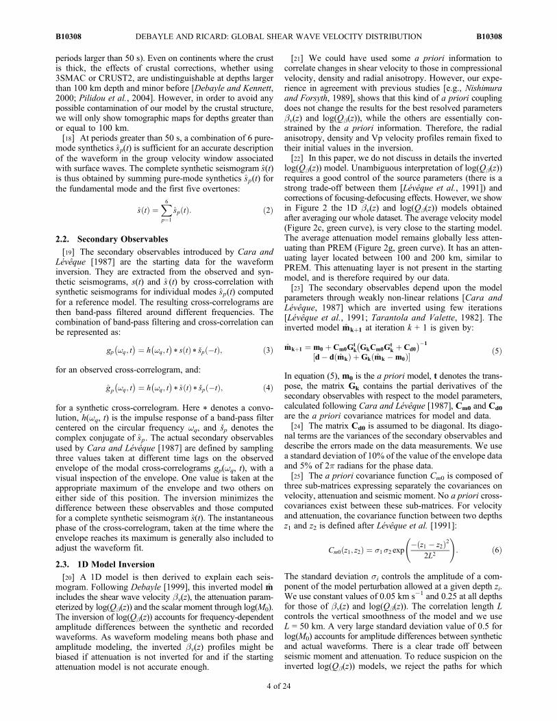
The agreement between DR2012 and S362ANI is there-fore very good over the range of wavelengths resolved byS362ANI. At 150 km depth, the correlation with HMSL isabove the 95% confidence level up to degree 22, and staysabove the 66% confidence level up to degree 28. This is afair result, considering that HMSL is based on a smallernumber of surface wave data (42,000 Rayleigh and 14,000Love waves) analyzed at longer periods (>66 s for HMSLcompared to >50 s in DR2012). S40RTS provides the bestagreement with DR2012 at 150 km depth. This is not sur-prising as the data sets used to constrain the uppermostmantle in both models are the most similar (several hundredof thousands of Rayleigh waveforms analyzed in the periodrange 50–250 s). In addition both inversion approaches,although different, allow for seismic heterogeneities up towavelengths of 1000 km. S40RTS and DR2012 correlateabove the 95% confidence level up to degrees 30–35 andremain above the 66% confidence levels up to degree 40.We consider this as a very encouraging result. It suggeststhat in spite of different approaches to extract informationfrom the seismograms and different strategies of inversion,it is now possible to build global tomographic models con-sistent up to degree 40 in the upper 200 km of the mantle.[70] At 250 km depth within the region just below the

lithosphere, DR2012 shows a weak correlation with othermodels even at low degree (Figure 12). This correlationstays above the 66% level only for a limited range of har-monic degrees (1–2 and 8–15 or 8–20 depending on theseismic model). For degrees 3 to 7, DR2012 is uncorrelatedwith the other seismic models. Therefore the pattern ofseismic anomalies in DR2012 differs from the other models,even at long wavelengths. We show in the next section thatDR2012 can be reconciled with other models by using alarger vertical degree of smoothing.

[71] Within the transition zone, correlations betweenDR2012 and the other seismic models are only significant atvery long wavelengths (Figure 12). At a depth of 500 km,DR2012 correlates with S40RTS at the 95% confidencelevel up to degree 8, falls below the 66% level for degree 9,then increases and remains above the 66% confidence up todegree 17. The correlation with S362ANI stays above the66% confidence up to degree 9 and the correlation withHMSL is poor. At the depth of 610 km, the correlationscurves show strong oscillations, likely due to oscillationspresent in the spectra at degrees smaller than 20. Theseoscillations, like those of the amplitudes (see Figure 11),suggest that the different models have a different degree-dependent sensibility at depth. S362ANI and S40RTS cor-relate with DR2012 above the 66% confidence level up todegree 8. Between degrees 8 and 15, the correlations oscil-late around the 66% level curve. Correlation curves withHMSL have strong oscillations and indicate a general pooragreement.[72] For completion, we discuss in Appendix B correla-

tions C(l ) obtained using successively S362ANI, S40RTSand HMSL as a reference model.

5.3. Effect of Vertical Smoothing

[73] Figures 13 (top) and 13 (middle) depict DR2012 andS40RTS at 250 km depth. Although DR2012 displays astrong correlation with surface tectonics at shallower depths(Figure 7), this correlation is already lost at 250 km depth.This correlation still holds for S40RTS, where high seismicvelocities beneath stable continents contrasts with low seis-mic velocities beneath most oceanic regions. At 250 kmdepth, HMSL and S362ANI (not shown) are similar toS40RTS and display the same correlation with surface tec-tonics. In DR2012, vertical smoothing is controlled by a

Figure 12. Correlations as a function of degree between DR2012 and S40RTS by Ritsema et al. [2011](blue line); HMSL by Houser et al. [2008] (green line); S362ANI by Kustowski et al. [2008] (red line).Correlations are computed at 150, 250, 500 and 610 km. In each plot the dotted and dashed lines indicatethe 95% and 66% significance levels respectively.


15 of 24

vertical correlation length (equation (6)) set to L = 50 km inthe waveform inversion. We tried a new waveform inver-sion of our entire dataset using a value of L = 100 km. Allother a priori parameters and criteria to accept or reject awaveform remain the same. With L = 100 km, the numberof records which pass successfully all stages of the wave-form inversion decreases to 348,995 (374,897 records weresuccessful using L = 50 km). Therefore, smoother pathaverage models are statistically less able to fulfill the samecriteria of waveform fit and of convergence towards aunique 1D model. Figure 13 (bottom) shows the pattern ofseismic heterogeneities at 250 km depth obtained using L =100 km which is now much more similar to S40RTS(Figure 13, middle) than with L = 50 km (Figure 13, top).At shallower depths, the L = 100 km model is very close to

DR2012. It is clear that imposing a priori a smoother ver-tical model is a simple way to reconcile our seismic modelwith other models. However, this is done at the price of a7% reduction in the number of waveforms that can beexplained. This is not dramatic, but we argue that this doesnot favor the smoothest model. Furthermore, the trace of theresolution matrix of the waveform inversion (see Table 1,last column) is consistently larger than 5 with only a weakdependence to L. Our data set is therefore able to beinverted for more than five layers in the shallowest uppermantle. A correlation length L = 50 km is thus a fair choiceto characterize the first 2L � tr(R) ≥ 500 km of the mantle.We therefore consider DR2012, built using L = 50 km asour preferred model, and the difference with other modelsaround 250 km depth is mostly due to the slightly thinnercratons of our model.[74] Figure 14 displays the correlation at 250 km between

our smooth model, L = 100 km, and the three other seismicmodels. This figure confirms that increasing the verticalsmoothing is a simple way to reconcile our model with othermodels. Our smoother model now correlates above the 95%confidence level up to degree 20 with S362ANI and S40RTSand up to degree 10 with HMSL.

5.4. Possible Effects of Radial Anisotropyon the Thickness of Cratons

[75] DKP2005, our previous global tomographic model[Debayle et al., 2005], was built using an isotropic versionof PREM as starting model. In DR2012, the initial syntheticseismogram includes the radial anisotropy of PREM. Thedepth extent of cratons is similar in DKP2005 and DR2012,suggesting that accounting for the radial anisotropy ofPREM with Rayleigh waves only has little effect.[76] Inverting for radial anisotropy in the uppermost

mantle would require a simultaneous analysis of Love andRayleigh waves. From our experience, this would notchange significantly the thickness of the SV-wave highvelocity lid. In Debayle and Kennett [2000] we invertedsimultaneously a set of Love and Rayleigh waves and foundsignificant radial anisotropy with SH faster than SV down to

Figure 13. SV-wave velocity distribution at 250 km depth(in per cent relative to PREM) obtained using a vertical cor-relation length of (top) 50 km and (bottom) 100 km as com-pared with (middle) the SV wave distribution at the samedepth in S40RTS by Ritsema et al. [2011]. A longer correla-tion length enforces the similarity between S40RTS andDR2012.

Figure 14. Correlations at a depth of 250 km between a“smoothed” version of DR2012 (using a vertical correlationlength of 100 km in the waveform modeling) and S40RTS byRitsema et al. [2011] (blue line), S362ANI by Kustowskiet al. [2008] (red line) and HMSL by Houser et al. [2008](green line).


16 of 24

about 200 km beneath Australia, but no clear difference inthe thickness of the SV-wave high velocity lid compared toan isotropic inversion.[77] Finally, notice that models S40RTS, HMSL and

S362ANI all show a thicker cratonic lid than DR2012,although S40RTS results from isotropic inversion ofRayleigh waves, HMSL from isotropic inversion of bothLove and Rayleigh waves and S362ANI from anisotropicinversion of Love and Rayleigh waves. We conclude thatthe limited depth extent of the cratonic lithosphere in ourmodel is not a consequence of non inverting for the radialanisotropy.

6. Concluding Remarks

[78] Our extension of the Debayle [1999] automated inver-sion algorithm further divides the waveform modeling intoelementary steps. This gives more flexibility to the code,allowing a better selection of the robust information and abetter extraction of higher-modes.[79] Using the new scheme, we matched successfully

374,897 fundamental and higher-modes Rayleigh waveformswhich provide a global coverage of the upper mantle. Foreach waveform, the inversion extracts a path average elasticand anelastic model and the corresponding fundamental andhigher mode dispersion and attenuation curves. The dis-persion and attenuation curves provide a dataset for futurefinite-frequency inversion.[80] Compared to DKP2005, our new 3D SV-wave

velocity model DR2012 represents a significant improve-ment in the transition zone (see Figure 10). In the uppermost200 km of the mantle, some new features of DR2012 showa better agreement with surface tectonics, suggesting thatthe new scheme and the increased number of data, both

contribute to the improvement of SV-wave mapping atshallow depths.[81] A comparison of DR2012 with three other recent

seismic models (S40RTS, S362ANI and HMSL), empha-sizes that in the uppermost 200 km of the mantle, all modelscorrelate above the 95% confidence level up to harmonicdegree 20. DR2012 and S40RTS which are the most similarin terms of datasets and of horizontal wavelengths allowedin the inversion, are also the most similar models. These twomodels correlate above the 95% and 66% confidence levelsup to degree 35 and 40 respectively. This is an encouragingresult, proving that in spite of different approaches to extractinformation from the seismograms and to invert for thisinformation, it is now possible to build global tomographicmodels consistent up to degree 40 in the uppermost 200 kmof the mantle.[82] The region between 200 km depth and the top of the

transition zone is an intermediate region where the verystrong heterogeneities present in the upper 200 km pro-gressively vanish. Continental roots disappear between 200and 250 km in DR2012, at a shallowest depth than in othermodels. It is possible to obtain thicker continental roots inDR2012 by imposing a priori smoother vertical variations.This does not seem required by the resolution of the wave-form inversion and leads to a less successful waveforminversion.[83] Within the transition zone, correlations between

DR2012 and other models are significant only up to degree 10.In this depth range, all models image a broad scale highvelocity signature around Indonesia and the Pacific, sug-gesting some “ponding” of the slabs.[84] To illustrate the agreement between two well corre-

lated models, we show in Figure 15 DR2012 and S40RTS

Figure 15. SV-wave perturbations (in per cent relative to PREM) at (top) 150 km and (bottom) 500 kmdepths in DR2012, compared with maps at the same depth in S40RTS by Ritsema et al. [2011].


17 of 24

at 150 and 500 km depth. Although at 150 km depth, thetwo models agree above the 95% confidence level up todegree 35, differences of few percents persist over wave-lengths greater than 1200 km both in continental (e.g. EastAsia) and oceanic (e.g. South Pacific) regions. Within thetransition zone, small scale heterogeneities are generally notcorrelated. By applying more sophisticated finite frequencytheory on the datasets which have been used to build thecurrent seismic models, we may add more details in themodels, but it is unlikely that we will remove their differ-ences at long wavelengths where the ray theory remains anexcellent approximation.[85] For these reason, we believe that we first need to

improve current seismic models. For DR2012, a first step isto complete our surface wave dataset with available longperiod S-wave datasets [e.g., from Zaroli et al., 2010] andwith normal mode measurements in order to map the entiremantle. Then, by exploiting our new set of dispersion andattenuation curves, we hope to built consistent 3D shearvelocity and quality factor models. This will contribute to

disentangle the thermal and compositional structures of themantle.

Appendix A: Description of the New AutomatedScheme

A1. Automatic Selection of the Secondary Observables

[86] In this section we describe how we sample the modalenvelopes at a given period to improve higher-modeextraction.[87] An example is presented in Figure A1 for the event

of February 13, 2008, located in Oaxaca, Mexico (16.35�S;�94.51�E) and recorded at station CAN in Canberra,Australia. For this intermediate depth event (87.1 km),a dominant fundamental mode is observed between 3.5 and4 km s�1 on the actual signal (bottom part of the figure),while the less energetic overtones have higher group veloci-ties. The initial synthetic seismogram is more energetic(it has been multiplied by a factor of 0.22 in Figure A1) andclearly the residual is huge.

Figure A1. Situation before waveform inversion for the February 13, 2008 event recorded at stationCAN (Canberra, Australia). The lower part of the figure shows: the observed seismogram (labeled “data”),the synthetic seismogram computed for the initial model (“initial”) and their difference (“residual”).The upper part shows the envelope of the filtered cross-correlogram functions gp(wq, t) for modes rangingfrom the fundamental mode (0) up to the fifth overtones and for filters centered from 50 (left) to 250 s(right) periods. For each mode and each period the lower functions are the envelope of the actual cross-correlogram functions (labeled “data”) while the upper functions are the envelope of the syntheticcross-correlogram functions (labeled “synt”). The vertical marks on the envelopes indicate where theactual envelopes are sampled for the inversion.


18 of 24

[88] In the top part of Figure A1, the modal envelopes ofthe synthetic (labeled “synth”) and actual (labeled “data”)cross-correlograms are shown for the 5 periods correspondingto the central periods of the gaussian filters h(wq, t) and forthe number of modes Nmode considered at each period (twomodes are enough for an accurate description of the signalat 250 s, six modes are needed at 75 and 50 s). The actualenvelopes result from the cross-correlation between the actualseismogram and each mode of a synthetic seismogram com-puted for a reference, initial model (see equation (3)). Thefilters h(wq, t) are gaussian in frequency and their width at�30 dB (3% of the maximum) is equal to their centralfrequency wq. The spacing of the central frequencies isequal to half the gaussian width at �30 dB, so that thefollowing sequence of central periods is chosen: 250, 165,110, 75 and 50 s. This choice allows us to cover the periodrange 50–250 s with weakly correlated secondary obser-vables (Figure A2), so that the data covariance matrix canbe considered as diagonal.[89] For mode 0, the actual seismogram is cross-correlated

with the fundamental mode of the reference synthetic seis-mogram. At 250 s period, higher modes are poorly excited.The actual envelope has a single lobe associated with themost energetic fundamental mode. At shorter periods, theactual envelopes have several maxima corresponding to dif-ferent alignments of the cross-correlated signals. The largestmaximum on each actual envelope is produced by the cross-correlation of the dominant fundamental mode of the actualand synthetic seismograms. It is found in the center of thediagram, close to the reference time t0 = 0 for which there isno delay between the cross-correlated signals. This is due tothe small difference in arrival time between the fundamentalmode of the synthetic and actual signals. The less energeticovertones of the actual seismogram produce secondary lobeswith a delay time corresponding to the delay between theovertones of the actual seismogram and the fundamentalmode of the reference synthetic.[90] For modes p = 1 to 5, the actual seismogram is

cross-correlated with mode p of the reference syntheticseismogram. The energetic fundamental mode of the actualseismogram still dominates the amplitude of the envelope,but the corresponding lobe is shifted. It is found at a delaytime corresponding to the delay between the fundamentalmode of the actual seismogram and the overtones of thesynthetic. The less energetic overtones of the actual seis-mogram produce secondary lobes close to the time t0 = 0

because the reference model gives a fair prediction of thearrival time of the overtones.[91] Figure A1 shows that for multimode seismograms,

the modal cross-correlogram functions have a complexshape, with several maxima related to the different modespresent in the signal. In addition, when a mode j is clearlydominant in the signal (e.g. the fundamental mode for ashallow event) it often contaminates the gp(wq, t) functionsand provides the largest maximum of the envelope evenwhen p ≠ j. Therefore, by sampling three points on thelargest maximum of each actual envelope, there is a risk ofextracting redundant information on the dominant mode,while loosing the information on the other modes.[92] To overcome this problem, Debayle [1999] over-

parameterizes the cross-correlation information. When theshape of the envelope has several maxima, Debayle [1999]selects the two best lobes, using the ratio Amax/|tmax � t0|as a criterion, where Amax is the amplitude of the maximumlocated at time tmax and t0 the reference time. This criterionfavors the largest lobes close to t0, where the current mode isexpected. By selecting two lobes, Debayle [1999] reducesthe risk of extracting redundant information on the domi-nant mode. The new scheme selects up to Nmode lobes,corresponding to the Nmode possible modes which interfereon each envelope.[93] During steps 1 to Nper (where Nper is the number of

selected band-pass filters as defined in section 3.1), theautomated code matches the envelopes of the cross correlo-grams. At a given period, the code first extracts a numberNsl ≤ Nmode of significant maxima for each modal envelope.A maximum is considered to be significant when itsamplitude is larger than Rmax = 6 times the average of theminima of the envelope. The selected maxima are thenranked according a decreasing Amax/|tmax � t0| criterion. Theinversion starts with all the first lobes of the modal envel-opes. Three iterations are allowed to deal with the weaknon-linearity of the secondary observables. Then a secondlobe is added on each modal envelopes for which it is foundto be significant and three new iterations are allowed tosimultaneously match the first and second lobes. This pro-cess is repeated until all the significant lobes have beenselected and inverted.[94] At this stage, the automated code decides, based on

the criteria given in the next section, whether it:[95] 1. adds the next shorter period[96] 2. adds iterations and follow the inversion of the

current dataset to complete convergence (a maximum of18 iterations is allowed to match the current period)[97] 3. steps back and redo the inversion of the current

period using a more severe criterion to select the envelopesmaxima (the criterion Rmax is incremented by 1).[98] During steps Nper + 1 to 2Nper the code matches the

instantaneous phase, taken at the time where the highestAmax/|tmax � t0| value has been found (i.e. when the first lobeof each envelope reaches its maximum). The algorithmhas three iterations to match the phase at each period, so that3� Nper iterations are required to match all phase data. Onceall phase data have been matched, the waveform analysis iscompleted. The top part of Figure A3 shows the automatedselection of the envelope secondary observables achieved atthe end of step Nper for the 2008 February 13 event recordedat station CAN. The vertical marks on the actual envelopes

Figure A2. Five gaussian filters h(wq, t) used for the wave-form inversion. The width and central period (1/wq) are chosento cover the period range 50–250 s.


19 of 24

labeled “data” indicate the points where the cross-correlogramshave been sampled. The bottom part of Figure A3 showsthe observed, synthetic and residual seismograms at the lastiteration of the waveform inversion process, once the phaseof all cross-correlograms has been incorporated. All together,the inversion of the seismogram depicted in Figure A3matches 42 peak maxima (each of one described by 3 values)and 15 peak phases (not shown), which add up to a total of141 secondary variables. Our 3D seismic model DR2012,incorporates about 375,000 waveforms corresponding to atotal of about 20 million observations.

A2. Evaluation of the Waveform Inversion

[99] We use several criteria to evaluate the quality of awaveform inversion:[100] 1. A misfit criterion for the data:

cd ¼

ffiffiffiffiffiffiffiffiffiffiffiffiffiffiffiffiffiffiffiffiffiffiffiffiffiffiffiffiffiffiffiffiffiffiffiffiffi1

n

Xni

d i � dcisdi

!2vuut ; ðA1Þ

where di are the data (secondary observables) in number n,sdi their standard deviation, and dci the predicted data.[101] 2. A misfit criterion for the model:

cm ¼ffiffiffiffiffiffiffiffiffiffiffiffiffiffiffiffiffiffiffiffiffiffiffiffiffiffiffiffiffiffiffiffiffiffiffiffiffi1

p

Xpi

mi � m0i

smi

� �2s

; ðA2Þ

where mi are the model parameters in number p, smi theira priori standard deviations, andm0i the parameters describingthe a priori model m0.[102] 3. The ratio of energy between the residual and the

actual seismogram:

R1 ¼ E finres

EactualðA3Þ

where Eresfin is the energy of the residual signal at the final

iteration and Eactual is the energy of the actual signal.[103] 4. An energy reduction parameter:

R2 ¼ 1� E finres

Einitres

ðA4Þ

where E resinit is the energy of the residual signal between the

observed and initial synthetic seismogram.[104] Several conditions have to be fulfilled in order to

progress through the different steps of the waveforminversion.[105] 1. A seismogram is considered for waveform mod-

eling if the initial synthetic predicts the amplitude of the realseismogram within a factor of 10. A poorer amplitude pre-diction should indicate inappropriate source parameters.[106] 2. From steps 1 to Nper, we compute the misfit cri-

terion cd at the end of each step for different subsets of thedata. We compute cd

tot using all the secondary observables

Figure A3. Same as Figure A1 but after the waveform inversion.


20 of 24

from periods 1 to the current period and cdsp using all the

secondary observables of the last period processed (theshortest period) only. We also compute an individual misfitcdso, for each secondary observables of the shortest period.

We monitor cdmax, the largest value of cd

so. The process isallowed to start the following step only if the followingmisfit criteria is verified

cmaxd ≤ Tc ðA5Þ

and when convergence is achieved

Dmax ctotd ;csp

d

� �≤ TD ðA6Þ

where DX is the change of X between the two last iterations.In this study we use threshold values Tc = 3 and TD = 0.5.[107] If cd

max > Tc, we assume that some secondary observ-able cannot be fitted properly, suggesting that it should nothave been chosen. The automated code steps back, increasesRmax by 1 and restarts the automatic selection of the sec-ondary observables at the current period. Increasing Rmax

reduces the number of selected lobes at a given period. Theselection and inversion of secondary observables is refinedthrough this process, until the criteria cd

max ≤ Tc is reached.[108] Note that the criterion associated with TD, ensures that

the data fit would not significantly improve by adding furtheriterations. If the misfit criteria (equations (A5) and (A6))are not reached after a maximum of 18 iterations (withoutcounting erased iterations when the algorithm steps back) ata given period, the data is rejected.[109] 3. From steps Nper + 1 to 2Nper the code uses 3 itera-

tions per period to match the instantaneous phase of themodal cross-correlograms. The instantaneous phase is alwaystaken at the time corresponding to the maximum of the “first”lobe, according to the ranking described in section A1.A quality control on the phase adjustment is done throughthe waveform fit criteria computed at the end of the last

iteration. A phase shift that remains between the actual andsynthetic cross-correlograms produces a phase shift betweenthe actual and synthetic waveforms. If a significant phaseshift remains between the synthetic and observed wave-forms, the seismogram does not pass the waveform fit cri-teria described below and is therefore discarded.[110] 4. At the end of the last iteration we compute the two

energy reduction criteria R1 and R2 over 3 group velocitywindows. The first one, between 3.5 and 6 km s�1, coversthe fundamental mode and the higher-modes, the secondone, between 3.5 and 4.2 km s�1, covers mostly the funda-mental mode, while the third one, between 4.2 and 6 km s�1

covers mostly the higher-modes. We also use these groupvelocity windows to evaluate the ratio Eh/f of the higher-mode energy over the fundamental mode energy for theactual seismogram.[111] A waveform inversion is considered to be success-

ful if:[112] 1. The final model predicts a synthetic seismogram

in agreement with the recorded waveform. We use the fol-lowing waveform fit criteria:[113] (i) R1 must be smaller than 0.3 or R2 must be larger

than 90% over the group velocity window 3.5–6 km s�1.[114] (ii) when higher-modes, over the group velocity win-

dow of 4.2–6 km s�1, dominate the actual signal (Eh/f > 4),in addition to (i), we also require that restricted over thisspecific velocity window, R1 must be smaller than 0.3 or R2

must be larger than 90%[115] (iii) when the fundamental mode clearly dominates

the actual signal (Eh/f < 0.25) in addition to (i), R1 must besmaller than 0.3 or R2 must be larger than 90% over thegroup velocity windows 3.5–4.2 km s�1.[116] 2. The iterative process has converged toward a

unique model. Our experience shows that this condition isverified when cm does not change by more than 0.05between the two last iterations.

Figure B1. Same as Figure 12 but for correlations between S362ANI by Kustowski et al. [2008] andS40RTS by Ritsema et al. [2011] (blue line); HMSL by Houser et al. [2008] (green line); DR2012 (purpleline).


21 of 24

[117] The main steps of our automated scheme are sum-marized in Figure 3.

Appendix B: Correlation Using S362ANI, S40RTSand HMSL as Reference Models

[118] We depict in Figures B1–B3 the results obtainedusing successively S362ANI, S40RTS and HMSL as a ref-erence model for the computation of the correlations C(l ).

In the first 200 km DR2012 and S40RTS are the two modelsthat correlate best at all degree, but up to l = 20 the fourmodels perform equally. In the transition zone DR2012,S362ANI and S40RTS are in agreement up to degree 10 onlyand HMSL might be less resolved. Notice that the fact thatS362ANI, S40RTS and HMSL include normal modes and/orbody waves while our model does not, does not seem toincrease their mutual correlation at depth. Clearly DR2012is different from the three other models around 250 km depth.

Figure B3. Same as Figure 12 but for correlations between HMSL by Houser et al. [2008] and S362ANIby Kustowski et al. [2008] (red line); S40RTS by Ritsema et al. [2011] (blue line); DR2012 (purple line).

Figure B2. Same as Figure 12 but for correlations between S40RTS by Ritsema et al. [2011] and HMSLby Houser et al. [2008] (green line); S362ANI by Kustowski et al. [2008] (red line); DR2012 (purple line).


22 of 24

[119] Acknowledgments. This work was supported by the FrenchANR SEISGLOB ANR-11-BLANC-SIMI5-6-016-01. We thank the Irisand Geoscope data centers for providing broadband data. We also used datafrom several temporary experiments including various PASSCAL deploy-ments in the world, and the SKIPPY and KIMBA experiments in Australia.We thank Anne Paul for providing seismological data of the SIMBAADtemporary experiment in the Egean-Anatolia region. Data from otherFrench temporary experiments in Afar, French Polynesia and Tibet wereprovided by RESIF-SI, the new French data distribution system. Our tomo-graphic model, DR2012, is freely available on request to Eric Debayle.We thank Goran Ekstrom, an anonymous reviewer and the Associate Editorfor their constructive reviews.

ReferencesBarruol, G., D. Bosch, V. Clouard, E. Debayle, M. Doin, M. Godard,F. Fontaine, F. Masson, A. Tommasi, and C. Thoraval (2002), Polynesianlithosphere and upper mantle experiment (plume): The South Pacificsuperswell under investigation, Eos Trans. AGU, 83(45), 510–514.

Bassin, C., G. Laske, and G. Master (2000), The current limits of resolutionfor surface wave tomography in north america, Eos Trans. AGU, 81(48),Fall Meet. Suppl., Abstract S12A-03.

Beucler, E., and J. Montagner (2006), Computation of large anisotropicseismic heterogeneities (CLASH), Geophys. J. Int., 165(2), 447–468,doi:10.1111/j.1365-246X.2005.02813.x.

Beucler, E., E. Stutzmann, and J. Montagner (2003), Surface wave higher-mode phase velocity measurements using a roller-coaster-type algorithm,Geophys. J. Int., 155(1), 289–307.

Cara, M. (1979), Lateral variations of S-velocity in the upper mantle fromhigher Rayleigh modes, Geophys. J. R. Astron. Soc., 57(3), 649–670.

Cara, M., and J. Lévêque (1987), Waveform inversion using secondaryobservables, Geophys. Res. Lett., 14, 1046–1049.

Debayle, E. (1999), SV-wave azimuthal anisotropy in the Australian uppermantle: Preliminary results from automated Rayleigh waveform inver-sion, Geophys. J. Int., 137(3), 747–754.

Debayle, E., and B. Kennett (2000), Anisotropy in the Australasian uppermantle from Love and Rayleigh waveform inversion, Earth Planet. Sci.Lett., 184(1), 339–351.

Debayle, E., and M. Sambridge (2004), Inversion of massive surface wavedata sets: Model construction and resolution assessment, J. Geophys.Res., 109, B02316, doi:10.1029/2003JB002652.

Debayle, E., J. Lévêque, and M. Cara (2001), Seismic evidence for a deeplyrooted low-velocity anomaly in the upper mantle beneath the northeasternAfro/Arabian continent, Earth Planet. Sci. Lett., 193(3–4), 423–436.

Debayle, E., B. Kennett, and K. Priestley (2005), Global azimuthal seismicanisotropy and the unique plate-motion deformation of Australia, Nature,433(7025), 509–512, doi:10.1038/nature03247.

Doin, M., and L. Fleitout (1996), Thermal evolution of the oceanic litho-sphere: An alternative view, Earth Planet. Sci. Lett., 142(1–2), 121–136,doi:10.1016/0012-821X(96)00082-9.

Dziewonski, A., and D. Anderson (1981), Preliminary reference Earthmodel, Phys. Earth Planet. Inter., 25, 297–356.

Dziewonski, A., T. Chou, and J. Woodhouse (1981), Determination ofearthquake source parameters from waveform data for studies of globaland regional seismicity, J. Geophys. Res., 86(B4), 2825–2852, doi:10.1029/JB086iB04p02825.

Ekstrom, G. (2011), A global model of Love and Rayleigh surface wave dis-persion and anisotropy, 25–250 s, Geophys. J. Int., 187(3), 1668–1686,doi:10.1111/j.1365-246X.2011.05225.x.

Ekstrom, G., J. Tromp, and E. Larson (1997), Measurements and global mod-els of surface wave propagation, J. Geophys. Res., 102(B4), 8137–8157.

Ekstrom, G., M. Nettles, and A. M. Dziewonski (2012), The global CMTproject 2004–2010: Centroid-moment tensors for 13,017 earthquakes,Phys. Earth Planet. Inter., 200, 1–9, doi:10.1016/j.pepi.2012.04.002.

Forsyth, D. (1977), Evolution of upper mantle beneath mid-ocean ridges,Tectonophysics, 38(1–2), 89–118, doi:10.1016/0040-1951(77)90202-5.

Goutorbe, B. (2010), Combining seismically derived temperature with heatflow and bathymetry to constrain the thermal structure of oceanic litho-sphere, Earth Planet. Sci. Lett., 295(3–4), 390–400, doi:10.1016/j.epsl.2010.04.013.

Heintz, M., E. Debayle, and A. Vauchez (2005), Upper mantle structure ofthe South American continent and neighboring oceans from surface wavetomography, Tectonophysics, 406(1–2), 115–139, doi:10.1016/j.tecto.2005.05.006.

Houser, C., G. Masters, P. Shearer, and G. Laske (2008), Shear and com-pressional velocity models of the mantle from cluster analysis of long-period waveforms, Geophys. J. Int., 174(1), 195–212, doi:10.1111/j.1365-246X.2008.03763.x.

Jaupart, C., and J. Mareschal (1999), The thermal structure and thickness ofcontinental roots, Lithos, 48(1–4), 93–114, doi:10.1016/S0024-4937(99)00023-7.

Kanamori, H., and D. Anderson (1977), Importance of physical dispersionin surface-wave and free oscillation problems: Review, Rev. Geophys.,15(1), 105–112, doi:10.1029/RG015i001p00105.

Kustowski, B., G. Ekstrom, and A. M. Dziewonski (2008), Anisotropicshear-wave velocity structure of the Earth’s mantle: A global model,J. Geophys. Res., 113, B06306, doi:10.1029/2007JB005169.

Lebedev, S., G. Nolet, T. Meier, R. van der Hilst, and G. Masters (2005),Automated multimode inversion of surface and S waveforms, Geophys.J. Int., 162(3), 951–964, doi:10.1111/j.1365-246X.2005.02708.x.

Lestunff, Y., and Y. Ricard (1995), Topography and geoid due to litho-spheric mass anomalies, Geophys. J. Int., 122(3), 982–990, doi:10.1111/j.1365-246X.1995.tb06850.x.

Lévêque, J., M. Cara, and D. Rouland (1991), Waveform inversion of sur-face wave data: Test of a new tool for systematic investigation of uppermantle structures, Geophys. J. Int., 104, 561–581.

Lévêque, J., E. Debayle, and V. Maupin (1998), Anisotropy in the IndianOcean upper mantle from Rayleigh and Love waveform inversion,Geophys. J. Int., 133(3), 529–540.

Maggi, A., E. Debayle, K. Priestley, and G. Barruol (2006a), Multimodesurface waveform tomography of the Pacific Ocean: A closer look atthe lithospheric cooling signature, Geophys. J. Int., 166(3), 1384–1397,doi:10.1111/j.1365-246X.2006.03037.x.

Maggi, A., E. Debayle, K. Priestley, and G. Barruol (2006b), Azimuthalanisotropy of the Pacific region, Earth Planet. Sci. Lett., 250(1–2), 53–71,doi:10.1016/j.epsl.2006.07.010.

Marquering, H., R. Snieder, and G. Nolet (1996), Waveform inversion andthe significance of surface-wave mode coupling, Geophys. J. Int., 124,258–278.

Montagner, J. (1986), Regional three-dimensional structures using long-period surface waves, Ann. Geophys., 4, 283–294.

Müller, R., M. Sdrolias, C. Gaina, and W. Roest (2008), Age, spreadingrates and spreading symmetry of the world’s ocean crust, Geochem.Geophys. Geosyst., 9, Q04006, doi:10.1029/2007GC001743.

Nataf, H., and Y. Ricard (1995), 3SMAC: An a priori tomographic modelof the upper mantle based on geophysical modeling, Phys. Earth Planet.Inter., 95, 101–122.

Nettles, M., and A. M. Dziewonski (2008), Radially anisotropic shearvelocity structure of the upper mantle globally and beneath NorthAmerica, J. Geophys. Res., 113, B02303, doi:10.1029/2006JB004819.

Nishimura, C., and D. Forsyth (1989), The anisotropic structure of theupper mantle in the Pacific, Geophys. J., 96(2), 203–229, doi:10.1111/j.1365-246X.1989.tb04446.x.

Nolet, G. (1975), Higher Rayleigh modes in western-Europe, Geophys. Res.Lett., 2(2), 60–62.

Nolet, G. (1990), Partitioned waveform inversion and two dimensionalstructure under the network of autonomously recording seismographs,J. Geophys. Res., 95, 8499–8512.

Panning, M., and B. Romanowicz (2006), A three-dimensional radiallyanisotropic model of shear velocity in the whole mantle, Geophys. J. Int.,167(1), 361–379, doi:10.1111/j.1365-246X.2006.03100.x.

Pilidou, S., K. Priestley, O. Gudmundsson, and E. Debayle (2004), Uppermantle S-wave speed heterogeneity and anisotropy beneath the NorthAtlantic from regional surface wave tomography: The Iceland and Azoresplumes, Geophys. J. Int., 159(3), 1057–1076, doi:10.1111/j.1365-246X.2004.02462.x.

Pilidou, S., K. Priestley, E. Debayle, and O. Gudmundsson (2005),Rayleigh wave tomography in the North Atlantic: High resolution imagesof the Iceland, Azores and Eifel mantle plumes, Lithos, 79(3–4), 453–474,doi:10.1016/j.lithos.2004.09.012.

Priestley, K., E. Debayle, D. McKenzie, and S. Pilidou (2006), Upper man-tle structure of eastern Asia from multimode surface waveform tomogra-phy, J. Geophys. Res., 111, B10304, doi:10.1029/2005JB004082.

Priestley, K., D. McKenzie, E. Debayle, and S. Pilidou (2008), The Africanupper mantle and its relationship to tectonics and surface geology,Geophys. J. Int., 175(3), 1108–1126, doi:10.1111/j.1365-246X.2008.03951.x.

Ritsema, J., A. Deuss, H. J. van Heijst, and J. H. Woodhouse (2011),S40RTS: A degree-40 shear-velocity model for the mantle from newRayleigh wave dispersion, teleseismic traveltime and normal-modesplitting function measurements, Geophys. J. Int., 184(3), 1223–1236,doi:10.1111/j.1365-246X.2010.04884.x.

Ritzwoller, M. H., N. M. Shapiro, M. P. Barmin, and A. L. Levshin (2002),Global surface wave diffraction tomography, J. Geophys. Res., 107(B12),2335, doi:10.1029/2002JB001777.

Salaün, G., H. A. Pedersen, A. Paul, V. Farra, H. Karabulut, D. Hatzfeld, C.Papazachos, D. M. Childs, C. Pequegnat, and SIMBAAD Team (2012),High-resolution surface wave tomography beneath the Aegean-Anatolia


23 of 24

region: Constraints on upper-mantle structure, Geophys. J. Int., 190(1),406–420, doi:10.1111/j.1365-246X.2012.05483.x.

Sambridge, M. (1999), Geophysical inversion with a neighbourhoodalgorithm—I. Searching a parameter space, Geophys. J. Int., 138(2),479–494.

Sieminski, A., E. Debayle, and J. Lévêque (2003), Seismic evidence for deeplow-velocity anomalies in the transition zone beneath West Antarctica,Earth Planet. Sci. Lett., 216(4), 645–661, doi:10.1016/S0012-821X(03)00518-1.

Sieminski, A., J.-J. Lévêque, and E. Debayle (2004), Can finite-frequencyeffects be accounted for in ray theory surface wave tomography?,Geophys. Res. Lett., 31, L24614, doi:10.1029/2004GL021402.

Spetzler, J., and R. Snieder (2001), The effect of small-scale heterogeneityon the arrival time of waves, Geophys. J. Int., 145, 786–796.

Spetzler, J., J. Trampert, and R. Snieder (2002), The effect of scattering insurface wave tomography, Geophys. J. Int., 149(3), 755–767, doi:10.1046/j.1365-246X.2002.01683.x.

Stutzmann, E., and J. Montagner (1993), An inverse technique for retriev-ing higher mode phase-velocity and mantle structure, Geophys. J. Int.,113(3), 669–683.

Takeuchi, H., and M. Saito (1972), Seismic surface waves, in Methods inComputational Physics, vol. 11, edited by B. A. Bolt, pp. 217–295,Academic, New York.

Tanaka, S., D. Suetsugu, H. Shiobara, H. Sugioka, T. Kanazawa, Y. Fukao,G. Barruol, and D. Reymond (2009), On the vertical extent of thelarge low shear velocity province beneath the South Pacific Superswell,Geophys. Res. Lett., 36, L07305, doi:10.1029/2009GL037568.

Tarantola, A., and B. Valette (1982), Generalised nonlinear inverse pro-blems solved using the least square criterion, Rev. Geophys., 20,219–232.

Trampert, J., and J. Spetzler (2006), Surface wave tomography: Finite-frequency effects lost in the null space, Geophys. J. Int., 164(2),394–400, doi:10.1111/j.1365-246X.2006.02864.x.

Trampert, J., and J. Woodhouse (1995), Global phase velocity maps of Loveand Rayleigh waves between 40 and 150 seconds, Geophys. J. Int.,122, 675–690.

Turcotte, D., and G. Schubert (2002), Geodynamics, 2nd ed., CambridgeUniv. Press, Cambridge, U. K.

van Heijst, H., and J. Woodhouse (1997), Measuring surface-wave overtonephase velocities using a mode branch stripping technique, Geophys. J. Int.,131, 209–230.

van Heijst, H., and J. Woodhouse (1999), Global high-resolution phasevelocity distributions of overtone and fundamental-mode surface wavesdetermined by mode branch stripping, Geophys. J. Int., 137, 601–620.

Visser, K., S. Lebedev, J. Trampert, and B. L. N. Kennett (2007), GlobalLove wave overtone measurements, Geophys. Res. Lett., 34, L03302,doi:10.1029/2006GL028671.

Visser, K., J. Trampert, and B. L. N. Kennett (2008), Global anisotropicphase velocity maps for higher mode Love and Rayleigh waves, Geophys.J. Int., 172(3), 1016–1032, doi:10.1111/j.1365-246X.2007.03685.x.

Wolfe, C. J., S. C. Solomon, G. Laske, J. A. Collins, R. S. Detrick, J. A.Orcutt, D. Bercovici, and E. H. Hauri (2011), Mantle P-wave velocity struc-ture beneath the Hawaiian hotspot, Earth Planet. Sci. Lett., 303(3–4),267–280, doi:10.1016/j.epsl.2011.01.004.

Yoshizawa, K., and G. Ekstrom (2010), Automated multimode phase speedmeasurements for high-resolution regional-scale tomography: Applica-tion to North America, Geophys. J. Int., 183(3), 1538–1558, doi:10.1111/j.1365-246X.2010.04814.x.

Yoshizawa, K., and B. Kennett (2002), Determination of the influence zonefor surface wave paths, Geophys. J. Int., 149, 441–454.

Zaroli, C., E. Debayle, and M. Sambridge (2010), Frequency-dependenteffects on global S-wave traveltimes: Wavefront-healing, scattering andattenuation, Geophys. J. Int., 182(2), 1025–1042, doi:10.1111/j.1365-246X.2010.04667.x.

Zhang, Y., and T. Lay (1999), Evolution of oceanic upper mantle structure,Phys. Earth Planet. Inter., 114(1–2), 71–80, doi:10.1016/S0031-9201(99)00047-3.

Zhang, Y., and T. Tanimoto (1991), Global Love wave phase-velocityvariation and its significance to plate-tectonics, Phys. Earth Planet.Inter., 66(3–4), 160–202.


24 of 24

a global shear velocity model of the upper mantle from...

Documents