a global empirical gia model based on grace data

1

A global empirical GIA model based on GRACE data Yu Sun1, Riccardo E. M. Riva2 1Key Laboratory of Data Mining and Sharing of Ministration of Education, Fuzhou University, Fuzhou, China. 2Dept. of Geoscience and Remote Sensing, Delft University of Technology, Delft, The Netherlands

Correspondence to: Riccardo E. M. Riva ([email protected]) 5

Abstract. The effect of Glacial Isostatic Adjustment (GIA) on the shape and gravity of the Earth is usually described by

numerical models that simultaneously solve for glacial evolution and Earth’s rheology, being mainly constrained by the

geological evidence of local ice extent and global sea level, as well as by geodetic observations of Earth’s rotation.

In recent years, GPS and GRACE observations have often been used to improve those models, especially in the context of

regional studies. However, consistency issues between different regional models limit their ability to answer questions from 10

global scale geodesy. Examples are the closure of the sea level budget, the explanation of observed changes in Earth’s

rotation, and the determination of the origin of the Earth’s reference frame.

Here, we present a global empirical model of present-day GIA, solely based on GRACE data and on geoid fingerprints of

mass redistribution. We will show how the use of observations from a single space-borne platform, together with GIA

fingerprints based on different viscosity profiles, allows us to tackle the questions from global scale geodesy mentioned 15

above. We find that, in the GRACE era (2003-2016), freshwater exchange between land and oceans has caused global mean

sea level to rise by 1.5 ± 0.3 mm/yr, the geocentre to move by 0.5 mm/yr, and the Earth’s dynamic oblateness (J2) to increase

by 6.7 × 10-11/yr.

1 Introduction

The observation-based estimation of mass redistribution in the Earth’s water layer from regional to global scales has been 20

made possible in the last two decades by the Gravity Recovery and Climate Experiment (GRACE) satellite mission (Tapley

et al., 2004; Wouters et al., 2014).

However, since observations of time-variable gravity are intrinsically sensitive to any mass change, the contribution of the

solid earth needs to be removed. In particular, it is necessary to account for the effect of a few great earthquakes (Han et al.,

2013) and of glacial isostatic adjustment (GIA). The latter represents the delayed viscoelastic response of the Earth to past 25

glacial cycles (Peltier, 2004), and it is the only process relevant at global scales.

Historically, GIA has been investigated by means of numerical models that simultaneously solve for changes in the ice cover

over a glacial cycle, as well as for the Earth’s mechanical properties, in particular mantle viscosity. Those models are mainly

constrained by the geological evidence of past ice extent, by reconstructions of past sea level change, and by observations of

earth rotation (Nakiboglu and Lambeck, 1980; Peltier, 1982; Nakada and Lambeck, 1987). While those models aim at 30

https://doi.org/10.5194/esd-2019-40Preprint. Discussion started: 3 September 2019c© Author(s) 2019. CC BY 4.0 License.

2

understanding past glaciations and their effect on sea level and earth rotation, they might not be optimal for providing an

accurate correction for the solid earth contribution to GRACE observations. This is mainly due to the fact that available

observations are sparse in both space and time, which largely limits the complexity of GIA models, hence their accuracy. In

order to improve the ability of GIA models to reproduce present-day signals, they have been further constrained by geodetic

observations of vertical land motion (Peltier et al., 2015; Caron et al., 2017). Nonetheless, GIA model uncertainties are still 35

one of the main source of errors for, e.g., GRACE-based estimates of global mean ocean mass change (WCRP Global Sea

Level Budget Group, 2018).

An alternative approach to model the effect of present-day GIA makes use of satellite-based geodetic observations in order

to generate empirical (or data-driven) models. So far, those models have been tailored to regions that were covered by the

largest ice sheets, namely Antarctica, Northern Europe and North America (e.g., Riva et al., 2009; Hill et al., 2010; Simon et 40

al., 2017). Regional models allow to obtain an improved accuracy by relying on multiple datasets (e.g., GPS, GRACE,

satellite altimetry), without introducing consistency issues that usually arise when working with satellite data at global

scales, such as the problem of assuring mass conservation or of using a common reference frame. As a result, those models

typically do not allow to properly tackle global problems, such as the determination of total ocean mass change.

Here, we present results from an empirical GIA model solely based on GRACE data and on physical basis functions, 45

represented by geoid fingerprints of known sources of mass change. The fingerprint approach used in this study has been

initially proposed by Rietbroek et al. (2012) for sea level studies, and adapted by Sun et al. (2019) to study changes in the

Earth’s oblateness. This is the first time that the approach is used to specifically produce GIA model results.

2 Methods

2.1 Inversion 50

The method has been discussed in Sun et al. (2019). In summary, we construct about 150 fingerprints of geoid change

induced by unit mass variations of continental water, solving the sea level equation (Farrell and Clark, 1976) on a

compressible elastic earth based on the Preliminary Reference Earth Model (PREM, Dziewonski and Andersen, 1981). The

fingerprints are based on: individual drainage basins for the two ice sheets, glacier regions from the Global Land Ice

Measurements from Space (GLIMS) database (Kargel et al., 2014) and empirical orthogonal functions of land hydrology 55

(Rietbroek et al., 2016). Those fingerprints are fundamentally the same as in Sun et al. (2019), with minor updates: over the

ice sheets, we have merged a few neighbouring drainage basins that were providing anti-correlated solutions (Antarctica:

next to the East Antarctic Weddell Sea, and on the Northern Peninsula; Greenland: in the North East interior), we do not

model peripheral glaciers around the Greenland Ice Sheet, and we have added separate fingerprints for the Southern

Patagonia Ice Field and for Lake Victoria. 60

In addition, as in Sun et al. (2019), we define six fingerprints of geoid change induced by GIA over distinct sub-regions

(three for North America, two for Northern Europe, one for Antarctica), as well as an additional fingerprint for the effect of


3

GIA-induced changes in the position of the Earth’s rotation axis (True Polar Wander, TPW). More detail about the GIA

fingerprints is given below.

Through a least-square approach in the spectral domain, we simultaneously fit all fingerprints to CSR RL06 GRACE 65

monthly fields of geoid height changes from January 2003 to August 2016 (Save et al., 2018), with the additional constraint

that the GIA fingerprints have to follow a linear trend (i.e., that the GIA monthly variations are constant through the whole

timespan). The result is a time series of scaling factors that, once multiplied by the respective fingerprints and added

together, optimally reproduces the original GRACE fields. It is important to notice that we only use GRACE spherical

harmonic coefficients starting from degree 2 and order 1: in other words, we do not force the solution to fit GRACE 70

observations of changes in the Earth’s oblateness, as it will be discussed later.

The obtained set of scaled fingerprints allows to partition the total GRACE signal into a number of components, driven by

somehow independent processes: GIA, which is the main object of this study, as well as mass changes in the cryosphere and

in land hydrology. The ocean is considered to be passive, meaning that we assume the effect of internal mass redistribution

by ocean dynamics to be accurately removed by the ocean de-aliasing products used during GRACE data processing 75

(Dobslaw et al., 2017).

2.2 GIA fingerprints

GIA fingerprints are obtained from solving the sea level equation for a spherically symmetric, viscoelastic, incompressible

and non-rotating PREM earth (Kendall et al., 2005; Martinec et al., 2018).

For the Northern Hemisphere, we use two earth models and two ice histories, leading to four different solutions. As ice 80

history, we use either ICE-6G_C (Peltier et al., 2015) of GLAC1D (Tarasov et al., 2012) for North America, and either ICE-

6G_C or ANU (Lambeck et al., 2010) for Northern Europe. The earth models always have an upper mantle viscosity of

5x1020 Pa s; the two variants have either an elastic lithospheric thickness of 100 km in combination with a lower mantle

viscosity of 3x1021 Pa s (similar to VM5a), or a 90-km-thick lithosphere in combination with a lower mantle viscosity of 1022

Pa s (Mitrovica and Forte, 1997). 85

For Greenland, we have no dedicated fingerprint due expected small signals and to their spatial overlap with the signature of

present-day ice mass changes, hence we only account for the far-field effects of the former neighbouring ice sheets.

For Antarctica, we use a single fingerprint, based on ice history IJ05 (Ivins and James, 2005), in combination with a 65-km-

think elastic lithosphere, and a viscosity of 5x1020 Pa s and 1022 Pa s in the upper and lower mantle, respectively. This

Antarctic set-up showed very good agreement with the empirical GIA model of Riva et al. (2009). 90

Finally, we produce a TPW fingerprint by isolating the C21 and S21 spherical harmonic coefficients of each GIA model.


4

2.3 Low-degree solutions

As discussed in Sun et al. (2019) and mentioned above, the least-squares solution makes only use of GRACE observations

from spherical harmonic degree 2 and order 1. However, the GIA fingerprints are complete from degree 2 order 0, while the 95

land water fingerprints are complete from degree 1 order 0. Hence, even if observational constraints are not applied, the fact

that a single scaling factor is determined for each fingerprint implies that the inversion can also provide a solution for the

Earth’s oblateness (J2, related to degree 2 order 0) and geocentre motion (degree 1). J2 estimates are important because its

observations from GRACE are notoriously poor (Chen and Wilson, 2008), while geocentre motion cannot be directly

observed by GRACE, but it is necessary to accurately determine mass changes in the Earth’s water layer (Chen et al., 2005). 100

Another interesting signal is represented by TPW, since there is still no consensus in the community about the exact

implementation of the rotational feedback in GIA modelling (Peltier and Luthcke, 2009; Mitrovica and Wahr, 2011;

Martinec and Hagedoorn, 2014).

We use the GRACE degree 2 order 1 coefficients to scale the effect of GIA-induced TPW, under the assumption that the

rotational feedback will affect TPW magnitude rather than direction (visually confirmed from Milne and Mitrovica, 1998). 105

However, a long-term linear pole tide (towards about 64o W, see IERS Conventions 2010, v.1.2.0) is removed from the

GRACE observations in the processing phase (Bettadpur, 2018), which implies that our TPW solution will only represent the

deviation from this long-term polar motion.

Since we assume that the GRACE pole tide correction also removes part of the polar motion induced by the present-day

redistribution of continental waters, we do not include the rotational feedback in those fingerprints, and choose to consider as 110

noise some of the pole tide signal contained in the GRACE monthly solutions.

3 Results

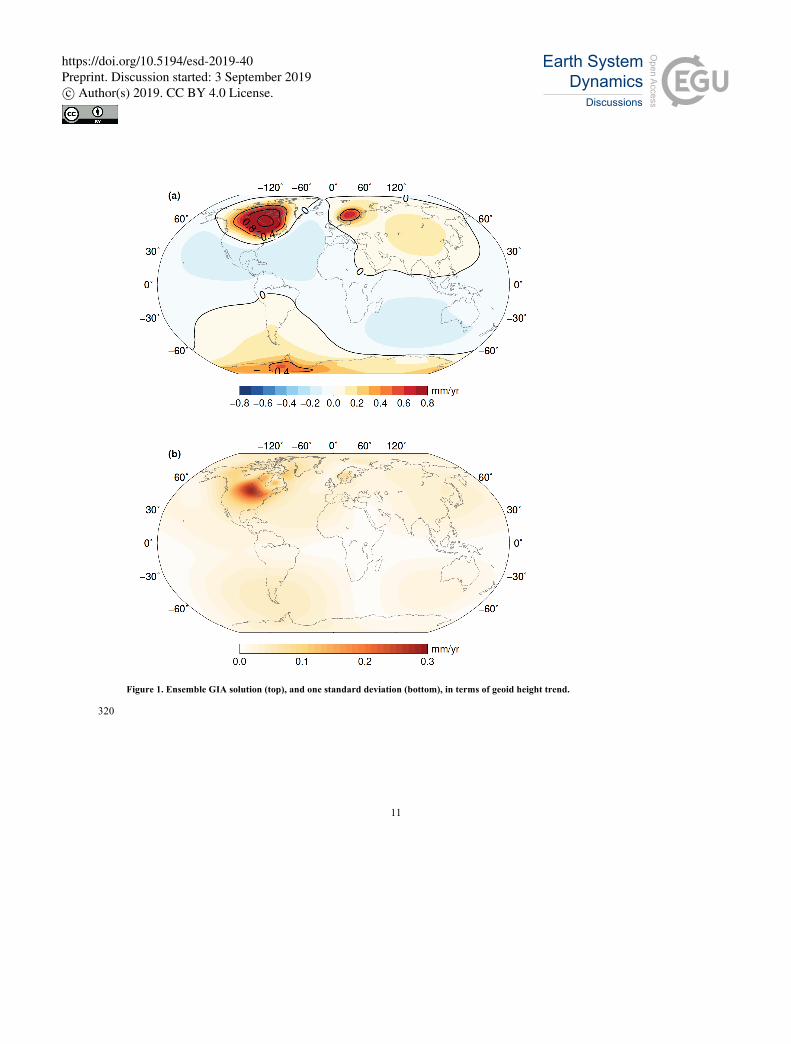
In Figure 1, we show the ensemble GIA solution and its standard deviation, obtained from averaging the four realizations

described above (two ice models, two earth models). The solution is represented in terms of geoid height changes,

consistently with the GRACE input. 115

In North America, the largest values are obtained over Hudson Bay and the overall pattern is rounder than ICE-6G_C

(VM5a), due to the influence of the GLAC1D ice history. The main difference between the two ice histories seems to lie in

the effect of ice sheet evolution at the south-west margin, resulting in a large uncertainty west of the Great Lakes.

The four models are rather similar over Northern Europe, as demonstrated by the small uncertainty. Notably, the ensemble

solution does not show any significant signal over the Barents Sea, apart from a NE extension of the 0.1 mm/y contour to 120

include Novaya Zemlya, reflecting the absence of signal in the input GRACE fields.

The solution over Antarctica, and in particular its minimal uncertainty, is a direct result of the use of a single fingerprint: in

principle, the approach allows for a variable Antarctic scaling, depending on the impact of alternative GIA fingerprints in the

northern hemisphere, but in practice the solution is dominated by the near-field regions.


5

Finally, a clear signal originates from the pole tide, i.e., the gravitational expression of TPW, which causes a positive trend 125

over Central Asia and southern South America, a negative trend over the southern Indian Ocean, and a southern extension of

the peripheral bulge over Central America. However, it should be noted that the magnitude of the pole motion of our solution

is about one third of the removed linear mean pole (0.37 deg/Ma against 1.07 deg/Ma), and its direction is considerably

different (88o W against 64o W).

130

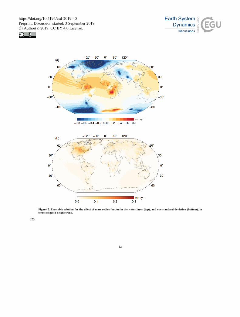
As discussed in the methods section, our approach also allows to quantify the contribution to GRACE from mass changes in

the Earth’s surface water layer. Results are shown in Figure 2.

The largest signals can be found over the two ice sheets and largely saturate the colour scale. In addition, some isolated

glacier regions are evidently losing mass, such as Alaska and Patagonia, while those neighbouring Greenland, such as the

Canadian Arctic and Iceland, are not directly distinguishable due to the low resolution of the geoid representation. A few 135

main regions of large land hydrological variation are also evident, such as the mass loss in the Caspian Sea and the Northern

India Plains, and the mass gain over the Zambezi River basins. The uncertainty is overall rather small, with the exception of

the region in North America that is also characterised by a large GIA uncertainty, due to the coupling of the GIA and

hydrology signals.

At large scales, the geoid rates are dominated by a large positive signal at low latitudes and by a diffused negative signal in 140

polar areas, mostly reflecting the global impact of polar ice melt on the Earth’s oblateness.

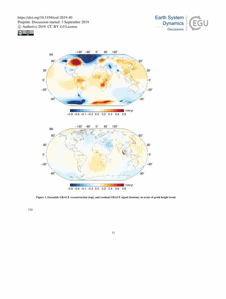
In Figure 3, we show the reconstructed signal (GIA + water layer) and its residual with respect to the original GRACE trend.

Particularly interesting is the plot of the residuals, in the bottom panel: apart from the clear signature of the 2004 Sumatra-

Andaman and of the 2011 Tohoku-Oki megathrust earthquakes, which we expressly do not model, most of the remaining 145

signals are at least one order of magnitude smaller than those in the reconstruction shown in the top panel. In the regions

characterised by the largest signals, the residuals are minimal, indicating that the chosen fingerprints are adequate to

reproduce the input GRACE fields.

At global scales, the main residual signal is represented by a rather round region over the SE Atlantic, which can be mostly

attributed to polar motion induced by mass redistribution in the water layer and not removed by the linear pole correction. 150

The additional effect of the inaccuracy of GRACE in determining changes in the Earth’s oblateness is likely the reason why

the largest residual is closer to the equator than the theoretical pole tide, and why it is part of a positive tropical band.

From the results that contribute to Figure 2, we can estimate global mean ocean mass changes due to individual sources.

Those values are listed in Table 1, and they are especially meant for validation of the ensemble solution. At the same time, 155

the uncertainties provide an indication of the role of GIA in GRACE-based estimates. The values for terrestrial water storage

(TWS), GIA, residual and all uncertainties are obtained from integrating the individual signals over all oceans, after

converting geoid changes into equivalent-water-height changes (Wahr et al., 1998), and excluding a 300-km-wide coastal


6

buffer zone. The values for the three ice sources are obtained from direct scaling of the original fingerprints, which avoids

possible biases from near-field sea-level changes (Sterenborg et al., 2013). We are comparing results against Frederikse et al. 160

(2019) and Bamber et al. (2018), in the following indicated as F19 and B18, respectively.

The global ocean mass change is slightly lower than the estimates by F19, though within reciprocal uncertainties. The

contributions of the individual ice sources are very close to the results by B18, where the largest contributor is Greenland,

followed by glaciers and Antarctica. Note that our Antarctic uncertainty is unrealistically small, as previously discussed, due

to the use of a single GIA fingerprint. The smallest contribution originates from TWS, which is about one third of the value 165

provided by F19, and just outside their 90% confidence level. Our estimate of the GIA contribution is at the low end of

previous estimates (e.g., Tamisiea, 2011), and characterised by a large uncertainty.

Notably, the residual signal is an order of magnitude smaller than the global mean ocean change and within its uncertainty,

confirming that we manage to capture most of the signature of present-day mass changes.

170

Finally, in Table 2, we list estimated trends of geocentre motion and Earth’s dynamic oblateness. The formers are only

provided for the water layer, since there are no benchmarked solutions we can rely upon to generate the corresponding GIA

fingerprints. Our result for geocentre motion in NS direction (Z component) is almost half a millimetre per year and

considerably larger than a few previous estimates (Sun et al., 2016b, Table 3).

As far as J2 is concerned, the total value of 4.1e-11/yr is in line with some solutions based on satellite laser ranging (Sośnica 175

et al., 2014) as well as to one of our previous solutions based on the GRACE-OBP approach (Sun et al., 2016a), though it

results from a smaller GIA and a larger water-layer contribution.

4 Discussion

The core of the proposed approach, and its main innovation with respect to the original work by Rietbroek et al. (2012), lies

in the assumption that the used set of fingerprints is sufficiently orthogonal to allow for a unique solution of the problem 180

based on a single set of observations, i.e., GRACE data. We expect this to be the case for signals due to mass redistribution

within the water layer, since the sources are small and sufficiently separated in the spatial domain. The problem becomes

more complex when mass change sources overlap in the spatial domain: in this case, the use of a single dataset could fail to

provide a unique solution. In particular, we are not able to solve for co-located GIA fingerprints, such as those that would

result from varying mantle viscosity for a given ice history. For this reason, we are producing different sets of GIA solutions, 185

each based on a single combination of ice histories and mantle viscosity, and average them afterwards. Similarly, we are not

able to use smaller GIA patches over the ice sheets, since their scale would become comparable to that of present-day ice

mass changes. Hence the choice of using a single GIA fingerprint for Antarctica and no GIA fingerprint at all for Greenland.

Working with overlapping signals would require the use of additional datasets and/or regularization methods (e.g., Wu et al,

2010; Rietbroek et al., 2016). In this study, we have chosen to adopt the simplest possible approach, by using only one 190


7

dataset and no additional regularization, with the aim of providing a robust solution in terms of internal consistency and of

global mass conservation, and of maintaining control on the impact of input data on the final solution.

A somehow separate issue is represented by the pole tide signal, which we are not trying to fully reconstruct due to the fact

that the GRACE trend is affected by the removal of a linear mean pole in the processing phase. However, this will mostly

affect the estimation of terrestrial water storage (Adhikari&Ivins, 2016), which is anyway very uncertain. 195

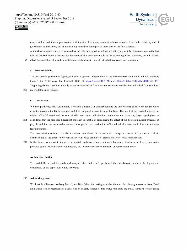
5 Data availability

The data used to generate all figures, as well as a spectral representation of the ensemble GIA solution, is publicly available

through the 4TU.Centre for Research Data at https://doi.org/10.4121/uuid:44326654-8dae-42df-adbd-d0f145581353.

Supporting datasets, such as monthly reconstructions of surface water redistribution and the four individual GIA solutions,

are available upon request. 200

6 Conclusions

We have partitioned GRACE monthly fields into a linear GIA contribution and the time-varying effect of the redistribution

of water masses at the Earth’s surface, and then computed a linear trend of the latter. The fact that the residual between the

original GRACE trend and the sum of GIA and water redistribution trends does not show any large signal gives us

confidence that the proposed fingerprint approach is capable of reproducing the effect of the different physical processes at 205

play. In addition, the estimated ocean mass change and the contributions of its individual sources are in line with the most

recent literature.

The uncertainties obtained for the individual contributors to ocean mass change are meant to provide a realistic

quantification of the global role of GIA in GRACE-based estimates of present-day water mass redistribution.

In the future, we expect to improve the spatial resolution of our empirical GIA model, thanks to the longer time series 210

provided by the GRACE Follow-On mission, and to a more advanced treatment of observational noise.

Author contribution

Y.S. and R.R. devised the study and analysed the results; Y.S. performed the calculations, produced the figures and

commented on the paper; R.R. wrote the paper.

Acknowledgements 215

We thank Lev Tarasov, Anthony Purcell, and Dick Peltier for making available their ice sheet history reconstructions; Pavel

Ditmar and Roelof Rietbroek for discussions on an early version of this study; John Ries and Mark Tamisiea for discussing


8

the impact of the GRACE pole tide correction; Matt King for commenting on geocentre motion. Y.S. is supported by the

National Natural Science Foundation of China (grant 41801393), the Education Department of Fujian Province (grant

JT180031), and Central Guide Local Science and Technology Development Project (grant 2017L3012). He is also partially 220

supported by the QiShan program of Fuzhou University. R.R. acknowledges funding from the Netherlands Organisation for

Scientific Research (NWO), through VIDI grant 864.12.012.

References

Adhikari, S., & Ivins, E. R.: Climate-driven polar motion: 2003–2015. Science advances, 2(4), e1501693, 2016. 225

Bamber, J. L., Westaway, R. M., Marzeion, B., & Wouters, B.: The land ice contribution to sea level during the satellite

era. Environmental Research Letters, 13(6), 063008, 2018.

Bettadpur, S.: GRACE 327-742, UTCSR Level-2 Processing Standards Document, https://podaac.jpl.nasa.gov/gravity/grace-

documentation, 2018.

Caron, L., Ivins, E. R., Larour, E., Adhikari, S., Nilsson, J., & Blewitt, G.: GIA model statistics for GRACE hydrology, 230

cryosphere, and ocean science. Geophysical Research Letters, 45(5), 2203-2212, 2018.

Chen, J. L., M. Rodell, C. R. Wilson, and J. S. Famiglietti: Low degree spherical harmonic influences on Gravity Recovery

and Climate Experiment (GRACE) water storage estimates, Geophys. Res. Lett., 32, L14405, 2005.

Chen, J. L.,& Wilson, C. R.: Low degree gravity changes from GRACE, Earth rotation, geophysical models, and satellite

laser ranging. Journal of Geophysical Research, 113, B06402, 2008. 235

Dobslaw, H., Bergmann-Wolf, I., Dill, R., Poropat, L., Thomas, M., Dahle, C., Esselborn, S., König, R., & Flechtner, F.: A

new high-resolution model of non-tidal atmosphere and ocean mass variability for de-aliasing of satellite gravity

observations: AOD1B RL06. Geophysical Journal International, 211(1), 263-269, 2017.

Dziewonski, A. M., & Anderson, D. L.: Preliminary reference Earth model. Physics of the earth and planetary

interiors, 25(4), 297-356, 1981. 240

Farrell, W. E., & Clark, J. A.: On postglacial sea level. Geophysical Journal International, 46(3), 647-667, 1976.

Frederikse, T., F. W. Landerer, & L. Caron: The imprints of contemporary mass redistribution on regional sea level and

vertical land motion observations. Solid Earth Discuss., doi: 10.5194/se-2018-128, 2019.

Han, S. C., Riva, R., Sauber, J., & Okal, E.: Source parameter inversion for recent great earthquakes from a decade-long

observation of global gravity fields. Journal of Geophysical Research: Solid Earth, 118(3), 1240-1267, 2013. 245

Hill, E. M., Davis, J. L., Tamisiea, M. E., & Lidberg, M.: Combination of geodetic observations and models for glacial

isostatic adjustment fields in Fennoscandia. Journal of Geophysical Research: Solid Earth, 115(B7), 2010.

Ivins, E. R., & James, T. S.: Antarctic glacial isostatic adjustment: a new assessment. Antarctic Science, 17(4), 541-553,

2005.


9

Kargel, J. S., Leonard, G. J., Bishop, M. P., Kääb, A., & Raup, B. H. (Eds.): Global land ice measurements from space. 250

Springer, 2014.

Kendall, R. A., Mitrovica, J. X., & Milne, G. A.: On post-glacial sea level–II. Numerical formulation and comparative

results on spherically symmetric models. Geophysical Journal International, 161(3), 679-706, 2005.

Lambeck, K., Purcell, A., Zhao, J., & Svensson, N. O.: The Scandinavian ice sheet: from MIS 4 to the end of the Last

Glacial Maximum. Boreas, 39(2), 410-435, 2010. 255

Martinec, Z., & Hagedoorn, J.: The rotational feedback on linear-momentum balance in glacial isostatic

adjustment. Geophysical Journal International, 199(3), 1823-1846, 2014.

Martinec, Z., Klemann, V., van der Wal, W., Riva, R. E. M., Spada, G., Sun, Y., ... & James, T. S.: A benchmark study of

numerical implementations of the sea level equation in GIA modelling. Geophysical Journal International, 215(1), 389-414,

2018. 260

Milne, G. A., & Mitrovica, J. X.: Postglacial sea-level change on a rotating Earth. Geophysical Journal

International, 133(1), 1-19, 1998.

Mitrovica, J. X., & Forte, A. M.: Radial profile of mantle viscosity: results from the joint inversion of convection and

postglacial rebound observables. Journal of Geophysical Research: Solid Earth, 102(B2), 2751-2769, 1997.

Mitrovica, J. X., & Wahr, J.: Ice age Earth rotation. Annual Review of Earth and Planetary Sciences, 39, 577-616, 2011. 265

Nakada, M., & Lambeck, K.: Glacial rebound and relative sea-level variations: a new appraisal. Geophysical Journal

International, 90(1), 171-224, 1987.

Nakiboglu, S. M., & Lambeck, K.: Deglaciation effects on the rotation of the Earth. Geophysical Journal

International, 62(1), 49-58, 1980.

Peltier, R.: Dynamics of the ice age Earth. In Advances in geophysics (Vol. 24, pp. 1-146). Elsevier, 1982. 270

Peltier, W. R.: Global glacial isostasy and the surface of the ice-age Earth: the ICE-5G (VM2) model and GRACE. Annu.

Rev. Earth Planet. Sci., 32, 111-149, 2004.

Peltier, W. R., Argus, D. F., & Drummond, R.: Space geodesy constrains ice age terminal deglaciation: The global ICE-

6G_C (VM5a) model. Journal of Geophysical Research: Solid Earth, 120(1), 450-487, 2015.

Peltier, W. R., & Luthcke, S. B.: On the origins of Earth rotation anomalies: New insights on the basis of both 275

‘‘paleogeodetic’’ data and Gravity Recovery and Climate Experiment (GRACE) data, J. Geophys. Res., 114, B11405, 2009.

Rietbroek, R., Brunnabend, S. E., Kusche, J., & Schröter, J.: Resolving sea level contributions by identifying fingerprints in

time-variable gravity and altimetry. Journal of Geodynamics, 59, 72-81, 2012.

Rietbroek, R., Brunnabend, S. E., Kusche, J., Schröter, J., & Dahle, C.: Revisiting the contemporary sea-level budget on

global and regional scales. Proceedings of the National Academy of Sciences, 113(6), 1504-1509, 2016. 280

Riva, R. E., Gunter, B. C., Urban, T. J., Vermeersen, B. L., Lindenbergh, R. C., Helsen, M. M., Bamber, J. L., van de Wal,

R. S. W., van den Broeke, M. R., & Schutz, B. E.: Glacial isostatic adjustment over Antarctica from combined ICESat and

GRACE satellite data. Earth and Planetary Science Letters, 288(3-4), 516-523, 2009.


10

Save, H., Tapley, B., & Bettadpur, S.: GRACE RL06 reprocessing and results from CSR. In EGU General Assembly

Conference Abstracts (Vol. 20, p. 10697), 2018. 285

Simon, K. M., Riva, R. E. M., Kleinherenbrink, M., & Tangdamrongsub, N.: A data-driven model for constraint of present-

day glacial isostatic adjustment in North America. Earth and Planetary Science Letters, 474, 322-333, 2017.

Sośnica, K., Jäggi, A., Thaller, D., Beutler, G., & Dach, R.: Contribution of Starlette, Stella, and AJISAI to the SLR-derived

global reference frame. Journal of geodesy, 88(8), 789-804, 2014.

Sterenborg, M. G., Morrow, E., & Mitrovica, J. X.: Bias in GRACE estimates of ice mass change due to accompanying sea-290

level change. Journal of Geodesy, 87(4), 387-392, 2013.

Sun, Y., Ditmar, P., & Riva, R.: Observed changes in the Earth’s dynamic oblateness from GRACE data and geophysical

models. Journal of geodesy, 90(1), 81-89, 2016a.

Sun, Y., R. Riva, and P. Ditmar: Optimizing estimates of annual variations and trends in geocenter motion and J2 from a

combination of GRACE data and geophysical models, J. Geophys. Res. Solid Earth, 121, 8352–8370, 2016b. 295

Sun, Y., Riva, R., Ditmar, P., & Rietbroek, R.: Using GRACE to Explain Variations in the Earth's Oblateness. Geophysical

Research Letters, 46(1), 158-168, 2019.

Tamisiea, M. E.: Ongoing glacial isostatic contributions to observations of sea level change. Geophysical Journal

International, 186(3), 1036-1044, 2011.

Tapley, B. D., Bettadpur, S., Ries, J. C., Thompson, P. F., & Watkins, M. M.: GRACE measurements of mass variability in 300

the Earth system. Science, 305(5683), 503-505, 2004.

Tarasov, L., Dyke, A. S., Neal, R. M., & Peltier, W. R.: A data-calibrated distribution of deglacial chronologies for the North

American ice complex from glaciological modeling. Earth and Planetary Science Letters, 315, 30-40, 2012.

Wahr, J., Molenaar, M., & Bryan, F.: Time variability of the Earth's gravity field: Hydrological and oceanic effects and their

possible detection using GRACE. Journal of Geophysical Research: Solid Earth, 103(B12), 30205-30229, 1998. 305

WCRP Global Sea Level Budget Group: Global sea-level budget 1993–present, Earth Syst. Sci. Data, 10, 1551-1590,

https://doi.org/10.5194/essd-10-1551-2018, 2018.

Wouters, B., Bonin, J. A., Chambers, D. P., Riva, R. E. M., Sasgen, I., & Wahr, J.: GRACE, time-varying gravity, Earth

system dynamics and climate change. Reports on Progress in Physics, 77(11), 116801, 2014.

Wu, X., Heflin, M. B., Schotman, H., Vermeersen, B. L., Dong, D., Gross, R. S., Ivins, E. R., Moore, A. W., & Owen, S. E.: 310

Simultaneous estimation of global present-day water transport and glacial isostatic adjustment. Nature Geoscience, 3(9),

642, 2010.

315


11

Figure 1. Ensemble GIA solution (top), and one standard deviation (bottom), in terms of geoid height trend.

320


12

Figure 2. Ensemble solution for the effect of mass redistribution in the water layer (top), and one standard deviation (bottom), in terms of geoid height trend.

325


13

Figure 3. Ensemble GRACE reconstruction (top), and residual GRACE signal (bottom), in terms of geoid height trend.

330


14

GMSL (mm/yr) Error (90%) Mass (Gt/yr)

Global ocean 1.46 [ 1.58 / - ] 0.28 -530 ± 100

Glaciers 0.54 [ 0.66 / 0.55 ] 0.12 -190 ± 40

Greenland 0.69 [ 0.80 / 0.71 ] 0.07 -250 ± 20

Antarctica 0.34 [ 0.40 / 0.31 ] 0.02 -120 ± 10

TWS -0.10 [-0.28 / - ] 0.23 40 ± 80

GIA -0.91 0.53 330 ± 190

Residual 0.21 0.34 -80 ± 120

Table 1. Estimated global mean ocean changes (Jan 2003 – Aug 2016), in terms of global mean sea level (GMSL) and mass, for the global ocean and for the individual contributors. Between brackets: values from Frederikse et al. (2019) and Bamber et al. (2018), respectively. Estimates from Bamber et al. (2018) are obtained from their Table 2, by averaging results over the three consecutive 335 time windows covering the GRACE era. We assume that 1 mm GMSL = -362 Gt, and we round off the mass estimates to the nearest ten.

GIA Water layer

X geocentre (mm/yr) - -0.05 ± 0.01

Y geocentre (mm/yr) - 0.15 ± 0.02

Z geocentre (mm/yr) - -0.46 ± 0.02

J2 (1e-11/yr) -2.6 ± 0.2 6.7 ± 0.1

Table 2. Estimated linear trends (Jan 2003 – Aug 2016) of geocentre motion and Earth’s dynamic oblateness. Errors represent the 340 90% confidence level.


a global empirical gia model based on grace data

Documents