a geometrical pore model for estimating the microscopical pore geometry of soil with infiltration...

Transport in Porous Media 54: 193–219, 2004.c© 2004 Kluwer Academic Publishers. Printed in the Netherlands. 193

A Geometrical Pore Model for Estimatingthe Microscopical Pore Geometry of Soilwith Infiltration Measurements

C. HAMMECKER1, L. BARBIERO1, P. BOIVIN1,2, J. L. MAEGHT1

and E. H. B. DIAW1,3

1Institut de Recherche pour le Developpement UR067, BP1386 Dakar, Senegal2Swiss Federal Institute for Technology, IATE-Pedology, 1015 Lausanne, Switzerland3Ecole Superieure Polytechnique, Thies, Senegal

(Received: 9 April 2002; in final form: 18 February 2003)

Abstract. This paper presents a simple geometrical pore model designed to relate characteristic poreradii of the porous network of soils with macroscopic infiltration parameters. The model composedof a stack of spherical hollow elements is described with two radii values: the pore access radiusand the actual pore radius. The model was compared to cylindrical pore models and its mathematicalconsistency was assessed. Soil sorptivity S and the second parameter A of the Philip infiltrationequation (1957), have been determined by numerically simulated infiltration. A diagram and anempirical relation have been set in order to relate the pore access and pore radii to the infiltrationparameters S and A. The consistency of the model was validated by comparing the predicted sorptiv-ity and hydraulic conductivity values, with the widely used unsaturated soil hydraulic functions (vanGenuchten, 1980). The model showed good agreement with experimental infiltration data, and it istherefore concluded that the use of a model with two radii improves the relation between microscopicpore size and macroscopic infiltration parameters.

Key words: sorptivity, gravity flow, pore size, disc infiltrometer, unsaturated soil hydraulicparameters.

Nomenclature

A second term of Richards’ infiltration equation (≈Ks) [L T−1].B empirical parameter [−].C integrating constant [M L2 T−1].D diffusivity [L2 T−1].e soil porosity [L3 L−3].f fluidity [L−1 T−1].g constant of gravity [L T−2].h height of conical element [L].hf soil water pressure head at the wetting front [L].I cumulative infiltration [L].k intrinsic permeability [L2].K hydraulic conductivity [L T−1].

194 C. HAMMECKER ET AL.

Ks saturated hydraulic conductivity [L T−1].K0 natural hydraulic conductivity [L T−1].l pore connectivity parameter [−].L capillary length [L].m,n empirical parameters [−].Pc capillary pressure [M L−1 T−2].r(z) varying meniscus radius [L].ra pore access radius [L].r∗c capillary tube radius [L].rret pore access radius determined on retention curve [L].R pore radius (widening) [L].Rret pore radius determined on retention curve [L].S sorptivity [L T−1/2].Se effective water content [−].t time [T].V volume [L3].z depth [L].

Greek lettersα empirical parameter [L−1].ε1, ε2 lower and upper limit of a single element [L].η dynamic viscosity [M L−1 T−1].θ water content [L3 L−3].θr, θs residual and saturated water content [L3 L−3].θx contact angle [−].λm frame-weighted mean pore size [L].ρ density [M L3].σ surface tension [M T−2].ψ matric suction head [L].

1. Introduction

It is well known that the pore size distribution in soils, strongly affects the in-filtration of water. Tillage and natural degradation processes such as crusteningor sodification drastically affect the pore structure in soils and consequently thehydraulic properties. Nevertheless there is little information on the actual relationbetween the dynamic of water infiltration and the microscopic pore structure ofsoils. Grismer (1986) studied the dependence of infiltration rate on changes in poresize distribution, with a special focus on the Green and Ampt (1911) equation.However the parameters necessary for the infiltration equations such as the poresize distribution index (Brooks and Corey, 1966) and the displacement pressurehead are difficult to determine experimentally. In this paper, we propose to use ageometrical pore model for which infiltration can be calculated with two pore radii(Hammecker et al., 1993; Hammecker and Jeannette, 1994). Conversely this modelcan be used to determine the effective pore size involved in infiltration processes,from experimentally measured sorptivity and constant infiltration rate. The aim ofthis study is to test the validity of the proposed model and the significance of the

GEOMETRIC PORE MODEL 195

two radii calculated from sorptivity and constant rate infiltration parameters, withthe proposed model.

This study is mainly focused on infiltration data derived from unsaturated hy-draulic parameters data from literature, but also on some infiltration results ob-tained with disc infiltrometers, as its use has become very common in soil science,for rapid in situ determination of saturated hydraulic conductivity, sorptivity, andother water flow parameters (Perroux and White, 1988; Smetten and Clothier,1989; Reynolds and Elrick, 1991; Thony et al., 1991).

2. Theory

2.1. THE MODEL

The geometry of the porous network in soils is far too complex to be completelydescribed mathematically. Nevertheless mercury porosimetry curves performed onseveral soil types, show that it is often possible to define a threshold in relation to apore size for which most of the porous network is interconnected (Dullien, 1979). Itcan then be assumed that water flow is mainly conducted through this kind of pore.A single pore radius is then selected. Most of the capillary imbibition or capillarypressure models involve simple pore shapes being defined as cylindrical, conical,sinusoidal or spherical (Kusakov and Nekrasov, 1966; van Brakel, 1975; Dullienet al., 1977; Levine et al., 1980; Marmur, 1989). The most common capillaryimbibition model is cylindrical, which is described by the Poiseuille law:

Q = πr∗c

4&P

8ηz= dV

dt= πr∗

c2 dz

dt(1)

⇒ dt = 8ηz

r∗c

2&Pdz (2)

whereQ is the water flow rate [L3 T−1] through the cylindrical tube of radius r∗c [L],

dV is the volume variation [L3], η is the dynamic viscosity of water [M L−1 T−1],&P is the pressure gradient [M L−1 T−2], and z [L] is the distance of the progress-ing meniscus from the free water level.

For downward flow (as found during in situ infiltration measurement), the driv-ing pressure gradient can be outlined as the sum of the capillary pressure Pc andthe gravitational pressure:

&P = Pc + ρgz (3)

For quasi-steady-state infiltration into a cylindrical tube, capillary pressure is givenby the Laplace law:

Pc = 2σ cos θxr∗

c

(4)


where σ is the surface tension [M T−2], θx is the contact angle (equal to 0◦ forwater on minerals), r∗

c [L] is the tube radius considered equivalent to the meniscusradius, ρ [M L−3] is the density of water and g [M S−2] is the gravitational constant.Although the Laplace equation has been defined for static equilibrium conditions,it has previously been used to describe dynamic imbibition processes by Washburn(1921). The validity of the use of this equation for dynamic imbibition processeshas been established by Dullien (1979) who compared it to the results of the moregeneral Navier–Stokes equations for the motion of fluid, and has been used byseveral authors (Peiris and Tennakone, 1980; Case, 1990, 1994). The analyticalsolution for the relation t (z), can be calculated by integrating (2) with (3) and (4):

t =[

z

r∗c

2ρg− 2σ

r∗c

3ρ2g2ln

(r∗

c2ρgz + 2σr∗

c

)+ C

]8η (5)

where C is an integrating constant, and for initial conditions t = 0 and z = 0 is:

C = 2σ

r∗c

3(ρg)2ln(2σr∗

c )

replacing it in Equation (5) leads to:

t =[

z

r∗c

2ρg− 2σ

r∗c

3ρ2g2ln

(1 + r∗

c ρgz

2σ

)]8η (6)

By posing:

K0 = ρgr∗c

2

8η(7a)

|hf| = 2σ

ρgr∗c

(7b)

Equation (6) becomes:

t = K−10

[z − |hf| ln

(1 + z

|hf|)]

(8)

In fact, this result generalises the Green–Ampt infiltration equation (Green andAmpt, 1911) from that obtained using a physical model of a porous medium,constituted of a bundle of cylindrical capillaries, where K0 [L T−1] is the ‘natural’saturated hydraulic conductivity (usually considered half the saturated hydraulicconductivity Ks), and |hf| [L] is the soil water pressure head at the wetting front.Equation (8) can be simplified and formulated in dimensionless form:

tD = zD ln(1 + zD)

where tD = tK0/|hf| and zD = z/|hf|. In this form the limits between capillary andgravity forces, are clearly defined for zD 1 and zD � 1 respectively.


Natural porous media such as rocks or soils have no well defined radius. How-ever it is possible to define a ‘hydraulic radius’ which is a macroscopic property ofthe media, for example, like the ratio of the volumetric water content and the sur-face area of the water solid interface, or an equivalent hydraulic pore radius whichdescribes the macroscopic infiltration properties of the medium, when introducedin Equation (6).

Nevertheless when realistic pore radius values for natural porous media areintroduced in Equation (6), the calculated imbibition kinetics are several order ofmagnitude higher than the experimental values (Dullien, 1979; Hammecker et al.,1993). The monotonous cylindrical pore shape, which is a poor representation ofthe porous network in soil, is mainly responsible for this discrepancy. The intro-duction of two parameters in Green–Ampt equation, partly solves this problemwith the introduction of a macroscopic parameter namely the ‘natural’ hydraulicconductivity (K0) and a microscopic parameter related to pore size distribution(|hf|). There is generally no direct relation between these two parameters unlikepresented previously for cylindrical capillary tubes (Eqs. (7a) and (7b)). Despitedescribing perfectly infiltration in natural soils, Equation (8) often shows non-uniqueness for parameter determination, when fitted to experimental infiltrationdata.

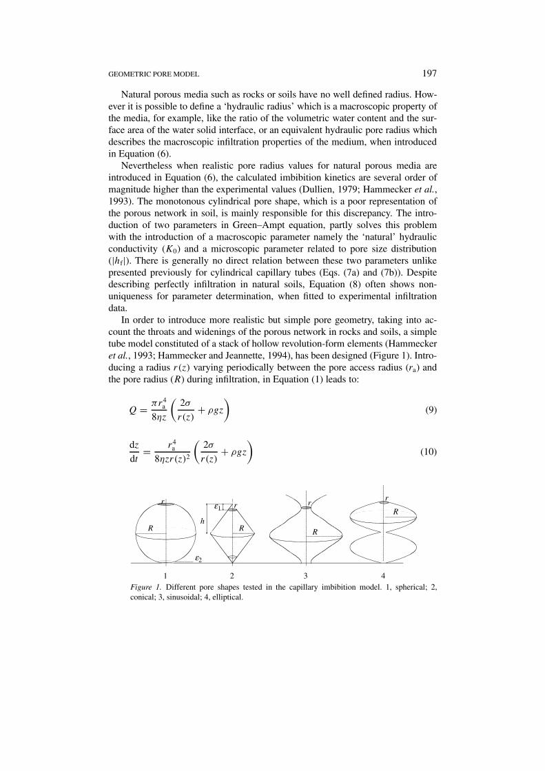
In order to introduce more realistic but simple pore geometry, taking into ac-count the throats and widenings of the porous network in rocks and soils, a simpletube model constituted of a stack of hollow revolution-form elements (Hammeckeret al., 1993; Hammecker and Jeannette, 1994), has been designed (Figure 1). Intro-ducing a radius r(z) varying periodically between the pore access radius (ra) andthe pore radius (R) during infiltration, in Equation (1) leads to:

Q = πr4a

8ηz

(2σ

r(z)+ ρgz

)(9)

dz

dt= r4

a

8ηzr(z)2

(2σ

r(z)+ ρgz

)(10)

Figure 1. Different pore shapes tested in the capillary imbibition model. 1, spherical; 2,conical; 3, sinusoidal; 4, elliptical.


It must be noticed that Hagen–Poiseuille equation defined for cylindrical tubes,is strictly speaking not valid to describe water transport in this kind of unit cell.This fact has been determined experimentally by Chavetau (1965) on millimetricto centimetric conical tubes. Hence an analogous equation has been considered todescribe water infiltration into a hollow element with varying radius (Eq. (9)). Inthis conceptual model, viscous and capillary forces are treated differently. In factviscous forces are supposed to be dependant on the pore access radius (ra) as flowthrough a hollow system is determined by the smallest section of the fluid path.Conductivity is consequently approximated by the conductivity of a cylinder ofradius equal to the pore access radius ra. On the other hand the capillary forces de-pend on the varying pore radius (r(z)) as the meniscus progresses along the hollowelement where the pore radius (R) determines the minimal capillary pressure.

For a single element, infiltration takes places between ε1 and ε2 corresponding,respectively, to the upper and lower limit, where the access orifice cuts through thepore (Figure 1). Their values are listed for different pore shapes in Table I. Thederivative imbibition function t (z) is:

dt = 8ηzr(z)2

r4a (2σ/r(z) + ρgz)

dz (11)

The integration of Equation (11) is solved numerically, by iterative calculation pro-cedures with a small dz incremental value set to (ε2−ε1)/1000. For each incrementdz, dt and t are recalculated with:

z =ε2∑ε1

dz (12)

t =∑

dt (13)

Table I. Pore radius equation for different pore shapesa

Model Equation ε1 ε2

Spherical r(z) = (2Rz − z2)1/2 R − (R2 − r2a )

1/2 R + (R2 − r2a )

1/2

Conical r(z) = zR/L, z < h (R − ra)L/R 2L − ε1

r(z) = R − ((z − L)R/L), z > h

Sinusoidal r(z) = ((R − ra)/2)× 0 L

×[1 + sin(2zπ/L)] + ra

Elliptical r(z) = ((R − ra)/2)× 0 L

×| sin(2zπ/L)| + ra

a R is the radius of the actual pore (the widening) and r is the radius of the access (the neck), h isthe height of some elements and ε1 and ε2 are, respectively, the superior and inferior limits of theshape.


For a tube of length Z constituted of a stack of n elements with Z = ∑nj (ε2 − ε1),

Equation (11) becomes:

dt = 8η(∑

(ε2 − ε1)j−1 + zj)r(zj )

2

r4a

(2σ/r(zj ) + ρg

(∑(ε2 − ε1)j−1 + zj

)) dz (14)

Indices j−1 refer to the number of the elements through which imbibition hasalready proceeded, and zj refers to the distance of the meniscus in the j th element.Considering the meniscus and the pore radius as being equivalent, r(z) can bereplaced in Equation (14) by any expression of Table I and the numerical integra-tion of this equation describes the function t (z) for the imbibition kinetics in theproposed tube model.

2.2. THEORETICAL VALIDATION

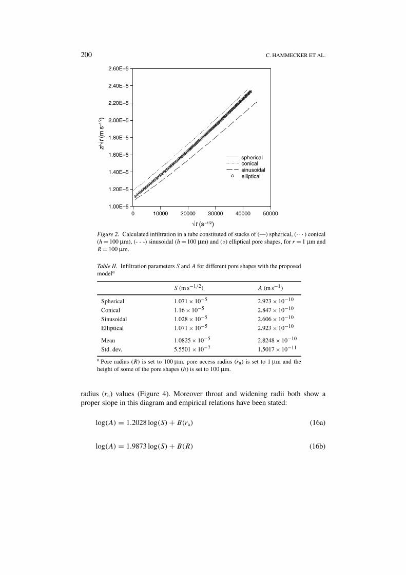
This model has been used to calculate the 1D infiltration into porous networks,with different pore geometry. According to the Philip 2-terms infiltration equationwhich is a truncated form of the power series solution of Philip (1957), sorptivity S

and the second infiltration parameter A have been determined for the numericallysimulated cumulative infiltration I :

I = St1/2 + At (15)

The parameters have been evaluated using the linear best fit relation of I/√t versus√

t , where A is the slope and S the ordinate at the origin (Figure 2). The results dis-played in Figure 2 and Table II, show that regardless of the actual pore shape of thepores, the infiltration kinetic is equivalent for identical pore and pore access radii.Moreover Figure 3 shows that for conical pore shape the height (h) of the elementis not determining infiltration when calculated with this conceptual model. Nev-ertheless it must be noticed that experimental data obtained by Chavetau (1965),show that conductivity in conical tubes is related inversely to the slope of the tubewalls, and that this kind of effect is not taken into account in this model. As theactual shape parameters are not relevant to the infiltration kinetics with this model,the spherical pore shape has been chosen for the following calculations.

On the other hand, these numerical results highlight that the dimensions ofthe pores (R and ra) are the critical parameters for imbibition. In order to testthe influence of both pore and pore-access radii on infiltration, calculations withvarying dimensions have been performed for 1 m long tubes (Z). The sorptivity(S) and the second infiltration rate (A) values have been determined, by linear bestfit as described previously.

For each pair; pore access radius – pore radius, a unique set of sorptivity andgravity flow is found. When plotted in a log–log diagram, A versus S show excel-lent linear correlation for constant widening radius values (R) and constant neck


Figure 2. Calculated infiltration in a tube constituted of stacks of (—) spherical, (· · · ) conical(h= 100 µm), (- - -) sinusoidal (h= 100 µm) and (◦) elliptical pore shapes, for r = 1 µm andR= 100 µm.

Table II. Infiltration parameters S and A for different pore shapes with the proposedmodela

S (m s−1/2) A (m s−1)

Spherical 1.071 × 10−5 2.923 × 10−10

Conical 1.16 × 10−5 2.847 × 10−10

Sinusoidal 1.028 × 10−5 2.606 × 10−10

Elliptical 1.071 × 10−5 2.923 × 10−10

Mean 1.0825 × 10−5 2.8248 × 10−10

Std. dev. 5.5501 × 10−7 1.5017 × 10−11

a Pore radius (R) is set to 100 µm, pore access radius (ra) is set to 1 µm and theheight of some of the pore shapes (h) is set to 100 µm.

radius (ra) values (Figure 4). Moreover throat and widening radii both show aproper slope in this diagram and empirical relations have been stated:

log(A) = 1.2028 log(S) + B(ra) (16a)

log(A) = 1.9873 log(S) + B(R) (16b)


Figure 3. Calculated downward infiltration kinetics, for a conical pore shape with differentheights h.

Figure 4. Calculated S and A values for different pore access radii (ra) and pore radii (R).

where the units are m s−1 for A, m s−1/2 for S and m for both the radii, R and ra.The ordinate at the origin for each equation, which depends on both throat andwidening radii, is determined empirically by second order best fit (Figure 5):

B(ra) = 0.0297(log(ra))2 + 1.6158 log(ra) + 5.4107 (17a)

B(R) = 0.091(log(R))2 + 1.9489 log(R)+ 6.7262 (17b)


Figure 5. Relation between ordinate at the origin of Equation (13) and the radii values forboth throat (ra) and widening (R).

Similarly by reversing Equations (16a), (16b), (17a) and (17b) both radii can becalculated from the infiltration parameters:

log(ra) = −1.6152 + (1.96802 − 0.14289 log(S) + 0.118 log(A))2

0.0594(18a)

log(R) = −1.9489 + (1.34987 − 0.72377 log(S) + 0.364 log(A))2

0.182(18b)

These equations defined for 10−6 � S � 10−1m s−0.5 and 10−14 �A� 10−1m s−1,show that sorptivity is more dependant on pore and pore access radius variationthan constant flow parameter, and that the relation between the hydraulic transferparameters and the internal pore topology is stronger for the pore radii (R) than forthe neck radii (ra).

In order to verify the validity of numerical procedure of the model, it has beentested at its limit where the pore radius and the throat radius are equal (R = ra)and the tube becomes cylindrical with analytical solutions (i.e. Eq. (5)). Moreover,the intrinsic permeability k [L2] of a single cylindrical tube can be calculated bycombining the Darcy Law and the Poiseuille law:

Q = kS&P

ηL= πr4

a&P

8ηL(19)

k = r2c

8(20)


where rc is the cylindrical tube radius. Hydraulic conductivity K [L T−1] relates tointrinsic permeability with fluidity f [L−1 T−1]:

K = kf (21)

f = ρg

η(22)

where ρ and η are, respectively, the density [M L−3] and the dynamic viscosity[M L−1 T−1] of water. Thus hydraulic conductivity can be expressed as function ofthe radius for a cylindrical tube:

K = r2c ρg

8η(23)

when K is reported in the log–log diagram, as a constant value for A, the calcu-lated conductivity for each tube radius rc, intercepts the corresponding line whererc = ra = R as shown in Figure 6. When calculating the capillary imbibitioninto a cylindrical tube for a given radius r∗

c (Eq. (2)), the two Philip parameterscan be determined by the same procedure as described previously, and reportedin Figure 6. Sorptivity and constant infiltration rate, respectively, are similar whenra = R = rc = r∗

c , whether derived from numerical calculation with the pro-posed model or from analytical solutions for imbibition and hydraulic conductivityof cylindrical tubes. This result illustrates the numerical consistency of the pro-posed model and of the calculation procedure. Lines for constant R/ra ratio can

Figure 6. Calculated S and A values for different pore and pore access values (R and r) withthe proposed model and calculated hydraulic conductivity values for cylindrical tubes.


Figure 7. Calculated S and A values for constant pore/pore access radii ratios.

be defined in the log(A) versus log(S) diagram (Figure 7), and consequently a‘restricted’ zone, for which the access radius would be bigger than the pore radius(R/ra < 1) is outlined. Hence for an homogeneous non-swelling soil, there aresorptivity and constant rate infiltration values which are not possible to be foundtogether for 1D infiltration (e.g. S/θ = 10−2 m s−1/2 and A/θ = 10−8 m s−1).

3. Material and Method

In order to evaluate the consistency of the proposed model it was compared to both,experimental infiltration data and theoretical unsaturated water flow models basedon the resolution of Richards’ equation (1931).

In fact it is essential to state the behaviour of this model compared to theclassical phenomenological infiltration models describing isothermal Darcian flowin porous bodies such as soils. Soil properties defined by the unsaturated soilhydraulic functions of van Genuchten (1980) have been used. For retention curves:

θ(ψ) = (θs − θr)(1 + |αψ |n)−m + θr, h < 0 (24a)

θ(ψ) = θs, ψ � 0 (24b)

and for hydraulic conductivity:

K(θ) = KsSle[1 − (1 − S1/m

e )m]2, ψ < 0 (25a)

K(θ) = Ks, ψ � 0 (25b)

where θr and θs denote the residual and the saturated water content [L3 L−3], ψ isthe matric pressure head [L], α [L−1], n [−] and m (1 − 1/n) [−] are empiricalparameters, Se is the effective water content ((θ − θr)/(θs − θr)), Ks is the saturatedhydraulic conductivity [L T−1] and l is the pore connectivity parameter [−]. The


predictive K(θ) model (Eqs. (25a) and (25b)) is based on the capillary theory ofMualem (1976) who found that in many soils an average value of 0.5 can be con-sidered for the pore connectivity parameter l. Despite being linked to the retentioncurve (Eqs. (24a) and (24b)), the description of hydraulic conductivity (Eqs. (25a)and (25b)) needs a supplementary parameter, namely the saturated hydraulic con-ductivity (Ks). This parameter is either measured experimentally or derived fromthe pore size distribution when experimental data are not available.

According to the Laplace equation (Eq. (4)), pressure head can be expressedas an equivalent pore radius. Consequently a pore size distribution can be de-rived from Equations (24a) and (24b), where α is proportional to the pore sizeand n is proportional to the homogeneity of the pore size distribution. Marshall(1958) proposed a statistical pore size distribution model predicting the saturatedhydraulic conductivity. It is based on the subdivision of the retention curve into afinite number m0 of parts of equal volume. Each one being characterised by a poreradius.

Ks = e2

8η2

m0∑i=1

((2i − 1)r2i ) (26)

where e is the porosity of the soil (≡ θs), ri is the mean pore radii (decreasing poreradii with increasing i) in each of the m0 parts in which the porous medium hasbeen divided.

However, attention must be drawn to the fact that Marshall’s model only prop-erly applies to poorly structured soils, where the main water flow takes placethrough the aggregates and that interaggregate water flow is negligible.

Infiltration in soil can then be calculated by numeric resolution of Richards’equation for given initial and limit conditions. However this procedure of calcula-tion is time consuming and the results need to be fitted by the Philips infiltrationequation (Eq. (15)). Alternatively, these infiltration parameters can be derived ana-lytically. The second rate of infiltration A can be assimilated to saturated hydraulicconductivity Ks, when infiltration time is long (Hillel, 1998).

Sorptivity S0, the second important water flow property for a soil, can be calcu-lated by combining Equations (24a), (24b), (25a) and (25b), according to Parlange(1975):

S20 =

∫ θ0

θn

(θ0 + θ − 2θn)D(θ) dθ (27)

where θn and θ0 are, respectively, initial and final water content and D(θ) thediffusivity [L2 T−1]:

D(θ) = K(θ)dψ

dθ(28)

Hence if the infiltration parameters like saturated hydraulic conductivity (Ks) andsorptivity (S0) for a soil are not known, they can be derived theoretically from itspore size distribution, described by Equations (24a) and (24b) and which is definedby four parameters (θr, θs, α and n).

206C

.HA

MM

EC

KE

RE

TA

L.

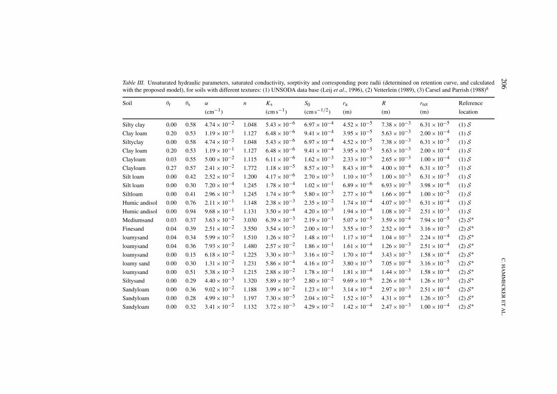
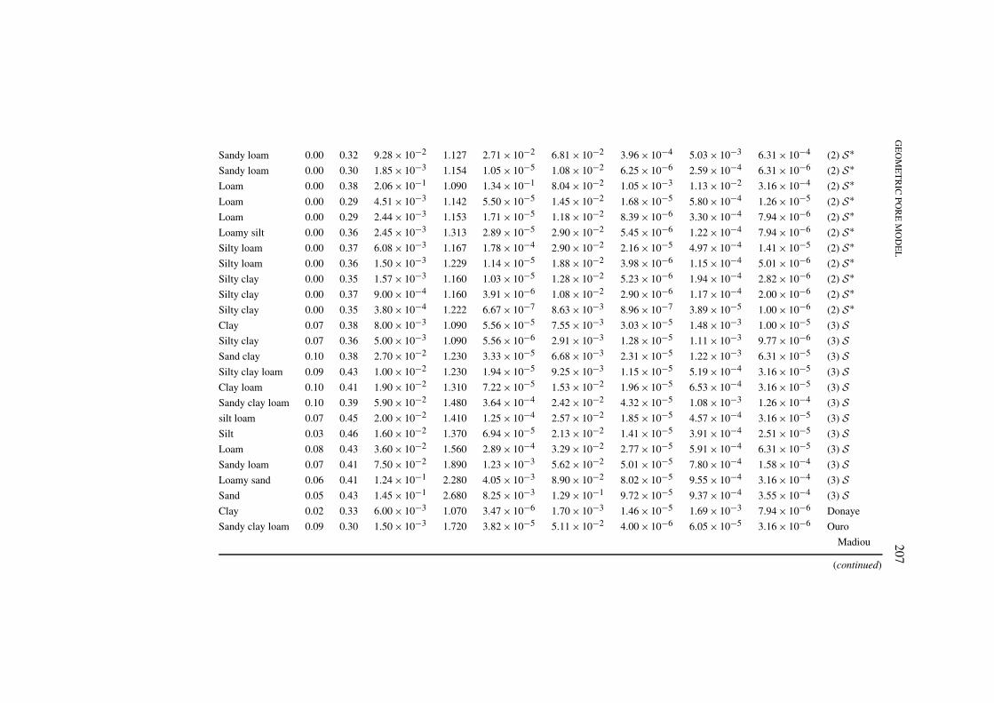
Table III. Unsaturated hydraulic parameters, saturated conductivity, sorptivity and corresponding pore radii (determined on retention curve, and calculatedwith the proposed model), for soils with different textures: (1) UNSODA data base (Leij et al., 1996), (2) Vetterlein (1989), (3) Carsel and Parrish (1988)a

Soil θr θs α n Ks S0 ra R rret Reference

(cm−1) (cm s−1) (cm s−1/2) (m) (m) (m) location

Silty clay 0.00 0.58 4.74 × 10−2 1.048 5.43 × 10−6 6.97 × 10−4 4.52 × 10−5 7.38 × 10−3 6.31 × 10−5 (1) SClay loam 0.20 0.53 1.19 × 10−1 1.127 6.48 × 10−6 9.41 × 10−4 3.95 × 10−5 5.63 × 10−3 2.00 × 10−4 (1) SSiltyclay 0.00 0.58 4.74 × 10−2 1.048 5.43 × 10−6 6.97 × 10−4 4.52 × 10−5 7.38 × 10−3 6.31 × 10−5 (1) SClay loam 0.20 0.53 1.19 × 10−1 1.127 6.48 × 10−6 9.41 × 10−4 3.95 × 10−5 5.63 × 10−3 2.00 × 10−4 (1) SClayloam 0.03 0.55 5.00 × 10−2 1.115 6.11 × 10−6 1.62 × 10−3 2.33 × 10−5 2.65 × 10−3 1.00 × 10−4 (1) SClayloam 0.27 0.57 2.41 × 10−2 1.772 1.18 × 10−5 8.57 × 10−3 8.43 × 10−6 4.00 × 10−4 6.31 × 10−5 (1) SSilt loam 0.00 0.42 2.52 × 10−2 1.200 4.17 × 10−6 2.70 × 10−3 1.10 × 10−5 1.00 × 10−3 6.31 × 10−5 (1) SSilt loam 0.00 0.30 7.20 × 10−4 1.245 1.78 × 10−4 1.02 × 10−1 6.89 × 10−6 6.93 × 10−5 3.98 × 10−6 (1) SSiltloam 0.00 0.41 2.96 × 10−3 1.245 1.74 × 10−6 5.80 × 10−3 2.77 × 10−6 1.66 × 10−4 1.00 × 10−5 (1) SHumic andisol 0.00 0.76 2.11 × 10−1 1.148 2.38 × 10−3 2.35 × 10−2 1.74 × 10−4 4.07 × 10−3 6.31 × 10−4 (1) SHumic andisol 0.00 0.94 9.68 × 10−1 1.131 3.50 × 10−4 4.20 × 10−3 1.94 × 10−4 1.08 × 10−2 2.51 × 10−3 (1) SMediumsand 0.03 0.37 3.63 × 10−2 3.030 6.39 × 10−3 2.19 × 10−1 5.07 × 10−5 3.59 × 10−4 7.94 × 10−5 (2) S∗Finesand 0.04 0.39 2.51 × 10−2 3.550 3.54 × 10−3 2.00 × 10−1 3.55 × 10−5 2.52 × 10−4 3.16 × 10−5 (2) S∗loamysand 0.04 0.34 5.99 × 10−2 1.510 1.26 × 10−2 1.48 × 10−1 1.17 × 10−4 1.04 × 10−3 2.24 × 10−4 (2) S∗loamysand 0.04 0.36 7.93 × 10−2 1.480 2.57 × 10−2 1.86 × 10−1 1.61 × 10−4 1.26 × 10−3 2.51 × 10−4 (2) S∗loamysand 0.00 0.15 6.18 × 10−2 1.225 3.30 × 10−3 3.16 × 10−2 1.70 × 10−4 3.43 × 10−3 1.58 × 10−4 (2) S∗loamy sand 0.00 0.30 1.31 × 10−2 1.231 5.86 × 10−4 4.16 × 10−2 3.80 × 10−5 7.05 × 10−4 3.16 × 10−5 (2) S∗loamysand 0.00 0.51 5.38 × 10−2 1.215 2.88 × 10−2 1.78 × 10−1 1.81 × 10−4 1.44 × 10−3 1.58 × 10−4 (2) S∗Siltysand 0.00 0.29 4.40 × 10−3 1.320 5.89 × 10−5 2.80 × 10−2 9.69 × 10−6 2.26 × 10−4 1.26 × 10−5 (2) S∗Sandyloam 0.00 0.36 9.02 × 10−2 1.188 3.99 × 10−2 1.23 × 10−1 3.14 × 10−4 2.97 × 10−3 2.51 × 10−4 (2) S∗Sandyloam 0.00 0.28 4.99 × 10−3 1.197 7.30 × 10−5 2.04 × 10−2 1.52 × 10−5 4.31 × 10−4 1.26 × 10−5 (2) S∗Sandyloam 0.00 0.32 3.41 × 10−2 1.132 3.72 × 10−3 4.29 × 10−2 1.42 × 10−4 2.47 × 10−3 1.00 × 10−4 (2) S∗

GE

OM

ET

RIC

POR

EM

OD

EL

207

Sandy loam 0.00 0.32 9.28 × 10−2 1.127 2.71 × 10−2 6.81 × 10−2 3.96 × 10−4 5.03 × 10−3 6.31 × 10−4 (2) S∗Sandy loam 0.00 0.30 1.85 × 10−3 1.154 1.05 × 10−5 1.08 × 10−2 6.25 × 10−6 2.59 × 10−4 6.31 × 10−6 (2) S∗Loam 0.00 0.38 2.06 × 10−1 1.090 1.34 × 10−1 8.04 × 10−2 1.05 × 10−3 1.13 × 10−2 3.16 × 10−4 (2) S∗Loam 0.00 0.29 4.51 × 10−3 1.142 5.50 × 10−5 1.45 × 10−2 1.68 × 10−5 5.80 × 10−4 1.26 × 10−5 (2) S∗Loam 0.00 0.29 2.44 × 10−3 1.153 1.71 × 10−5 1.18 × 10−2 8.39 × 10−6 3.30 × 10−4 7.94 × 10−6 (2) S∗Loamy silt 0.00 0.36 2.45 × 10−3 1.313 2.89 × 10−5 2.90 × 10−2 5.45 × 10−6 1.22 × 10−4 7.94 × 10−6 (2) S∗Silty loam 0.00 0.37 6.08 × 10−3 1.167 1.78 × 10−4 2.90 × 10−2 2.16 × 10−5 4.97 × 10−4 1.41 × 10−5 (2) S∗Silty loam 0.00 0.36 1.50 × 10−3 1.229 1.14 × 10−5 1.88 × 10−2 3.98 × 10−6 1.15 × 10−4 5.01 × 10−6 (2) S∗Silty clay 0.00 0.35 1.57 × 10−3 1.160 1.03 × 10−5 1.28 × 10−2 5.23 × 10−6 1.94 × 10−4 2.82 × 10−6 (2) S∗Silty clay 0.00 0.37 9.00 × 10−4 1.160 3.91 × 10−6 1.08 × 10−2 2.90 × 10−6 1.17 × 10−4 2.00 × 10−6 (2) S∗Silty clay 0.00 0.35 3.80 × 10−4 1.222 6.67 × 10−7 8.63 × 10−3 8.96 × 10−7 3.89 × 10−5 1.00 × 10−6 (2) S∗Clay 0.07 0.38 8.00 × 10−3 1.090 5.56 × 10−5 7.55 × 10−3 3.03 × 10−5 1.48 × 10−3 1.00 × 10−5 (3) SSilty clay 0.07 0.36 5.00 × 10−3 1.090 5.56 × 10−6 2.91 × 10−3 1.28 × 10−5 1.11 × 10−3 9.77 × 10−6 (3) SSand clay 0.10 0.38 2.70 × 10−2 1.230 3.33 × 10−5 6.68 × 10−3 2.31 × 10−5 1.22 × 10−3 6.31 × 10−5 (3) SSilty clay loam 0.09 0.43 1.00 × 10−2 1.230 1.94 × 10−5 9.25 × 10−3 1.15 × 10−5 5.19 × 10−4 3.16 × 10−5 (3) SClay loam 0.10 0.41 1.90 × 10−2 1.310 7.22 × 10−5 1.53 × 10−2 1.96 × 10−5 6.53 × 10−4 3.16 × 10−5 (3) SSandy clay loam 0.10 0.39 5.90 × 10−2 1.480 3.64 × 10−4 2.42 × 10−2 4.32 × 10−5 1.08 × 10−3 1.26 × 10−4 (3) Ssilt loam 0.07 0.45 2.00 × 10−2 1.410 1.25 × 10−4 2.57 × 10−2 1.85 × 10−5 4.57 × 10−4 3.16 × 10−5 (3) SSilt 0.03 0.46 1.60 × 10−2 1.370 6.94 × 10−5 2.13 × 10−2 1.41 × 10−5 3.91 × 10−4 2.51 × 10−5 (3) SLoam 0.08 0.43 3.60 × 10−2 1.560 2.89 × 10−4 3.29 × 10−2 2.77 × 10−5 5.91 × 10−4 6.31 × 10−5 (3) SSandy loam 0.07 0.41 7.50 × 10−2 1.890 1.23 × 10−3 5.62 × 10−2 5.01 × 10−5 7.80 × 10−4 1.58 × 10−4 (3) SLoamy sand 0.06 0.41 1.24 × 10−1 2.280 4.05 × 10−3 8.90 × 10−2 8.02 × 10−5 9.55 × 10−4 3.16 × 10−4 (3) SSand 0.05 0.43 1.45 × 10−1 2.680 8.25 × 10−3 1.29 × 10−1 9.72 × 10−5 9.37 × 10−4 3.55 × 10−4 (3) SClay 0.02 0.33 6.00 × 10−3 1.070 3.47 × 10−6 1.70 × 10−3 1.46 × 10−5 1.69 × 10−3 7.94 × 10−6 Donaye

Sandy clay loam 0.09 0.30 1.50 × 10−3 1.720 3.82 × 10−5 5.11 × 10−2 4.00 × 10−6 6.05 × 10−5 3.16 × 10−6 Ouro

Madiou

(continued)

208C

.HA

MM

EC

KE

RE

TA

L.

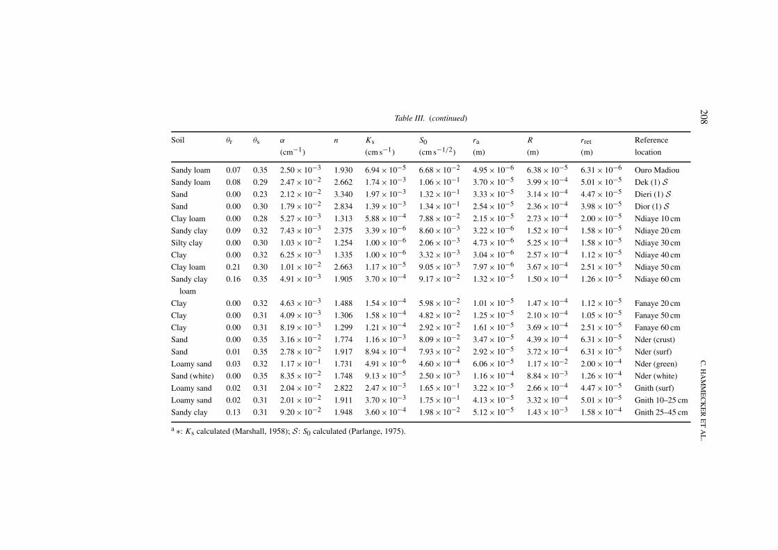
Table III. (continued)

Soil θr θs α n Ks S0 ra R rret Reference

(cm−1) (cm s−1) (cm s−1/2) (m) (m) (m) location

Sandy loam 0.07 0.35 2.50 × 10−3 1.930 6.94 × 10−5 6.68 × 10−2 4.95 × 10−6 6.38 × 10−5 6.31 × 10−6 Ouro Madiou

Sandy loam 0.08 0.29 2.47 × 10−2 2.662 1.74 × 10−3 1.06 × 10−1 3.70 × 10−5 3.99 × 10−4 5.01 × 10−5 Dek (1) SSand 0.00 0.23 2.12 × 10−2 3.340 1.97 × 10−3 1.32 × 10−1 3.33 × 10−5 3.14 × 10−4 4.47 × 10−5 Dieri (1) SSand 0.00 0.30 1.79 × 10−2 2.834 1.39 × 10−3 1.34 × 10−1 2.54 × 10−5 2.36 × 10−4 3.98 × 10−5 Dior (1) SClay loam 0.00 0.28 5.27 × 10−3 1.313 5.88 × 10−4 7.88 × 10−2 2.15 × 10−5 2.73 × 10−4 2.00 × 10−5 Ndiaye 10 cm

Sandy clay 0.09 0.32 7.43 × 10−3 2.375 3.39 × 10−6 8.60 × 10−3 3.22 × 10−6 1.52 × 10−4 1.58 × 10−5 Ndiaye 20 cm

Silty clay 0.00 0.30 1.03 × 10−2 1.254 1.00 × 10−6 2.06 × 10−3 4.73 × 10−6 5.25 × 10−4 1.58 × 10−5 Ndiaye 30 cm

Clay 0.00 0.32 6.25 × 10−3 1.335 1.00 × 10−6 3.32 × 10−3 3.04 × 10−6 2.57 × 10−4 1.12 × 10−5 Ndiaye 40 cm

Clay loam 0.21 0.30 1.01 × 10−2 2.663 1.17 × 10−5 9.05 × 10−3 7.97 × 10−6 3.67 × 10−4 2.51 × 10−5 Ndiaye 50 cm

Sandy clay 0.16 0.35 4.91 × 10−3 1.905 3.70 × 10−4 9.17 × 10−2 1.32 × 10−5 1.50 × 10−4 1.26 × 10−5 Ndiaye 60 cm

loam

Clay 0.00 0.32 4.63 × 10−3 1.488 1.54 × 10−4 5.98 × 10−2 1.01 × 10−5 1.47 × 10−4 1.12 × 10−5 Fanaye 20 cm

Clay 0.00 0.31 4.09 × 10−3 1.306 1.58 × 10−4 4.82 × 10−2 1.25 × 10−5 2.10 × 10−4 1.05 × 10−5 Fanaye 50 cm

Clay 0.00 0.31 8.19 × 10−3 1.299 1.21 × 10−4 2.92 × 10−2 1.61 × 10−5 3.69 × 10−4 2.51 × 10−5 Fanaye 60 cm

Sand 0.00 0.35 3.16 × 10−2 1.774 1.16 × 10−3 8.09 × 10−2 3.47 × 10−5 4.39 × 10−4 6.31 × 10−5 Nder (crust)

Sand 0.01 0.35 2.78 × 10−2 1.917 8.94 × 10−4 7.93 × 10−2 2.92 × 10−5 3.72 × 10−4 6.31 × 10−5 Nder (surf)

Loamy sand 0.03 0.32 1.17 × 10−1 1.731 4.91 × 10−6 4.60 × 10−4 6.06 × 10−5 1.17 × 10−2 2.00 × 10−4 Nder (green)

Sand (white) 0.00 0.35 8.35 × 10−2 1.748 9.13 × 10−5 2.50 × 10−3 1.16 × 10−4 8.84 × 10−3 1.26 × 10−4 Nder (white)

Loamy sand 0.02 0.31 2.04 × 10−2 2.822 2.47 × 10−3 1.65 × 10−1 3.22 × 10−5 2.66 × 10−4 4.47 × 10−5 Gnith (surf)

Loamy sand 0.02 0.31 2.01 × 10−2 1.911 3.70 × 10−3 1.75 × 10−1 4.13 × 10−5 3.32 × 10−4 5.01 × 10−5 Gnith 10–25 cm

Sandy clay 0.13 0.31 9.20 × 10−2 1.948 3.60 × 10−4 1.98 × 10−2 5.12 × 10−5 1.43 × 10−3 1.58 × 10−4 Gnith 25–45 cm

a ∗: Ks calculated (Marshall, 1958); S : S0 calculated (Parlange, 1975).


Unsaturated hydraulic function data, for soils with a wide range of texture, havebeen collected in the literature and used to test the model (Carsel and Parrish, 1988;Vetterlein, 1989; Leij et al., 1996) and displayed in Table III.

Experimentally determined infiltration parameters for soils of the river Senegalvalley (north of the Republic of Senegal) have equally been utilised for testingthe reliability of the model. The retention curves have been determined duringevaporation experiments according to Wind’s method (1968). The correspondingunsaturated soil hydraulic parameters were evaluated with RETC Code (vanGenuchten et al., 1991). Saturated hydraulic conductivity Ks and sorptivity S0

have been determined from field infiltration experiments performed with a discinfiltrometer for different pressure head values. Sorptivity has been evaluated fromthe transient infiltration flow, whereas saturated hydraulic conductivity has beenderived from the constant rate infiltration according to Wooding’s equation (1968)(Appendix A).

Common infiltration parameters like saturated hydraulic conductivity Ks andsorptivity S0, evaluated from a 3D infiltration experiment with a disc infiltrometer,can be used directly in this 1D flow model. As the infiltrations have been simu-lated over long time periods with the model, namely until reaching a cumulatedinfiltration depth of 1 m, the constant infiltration rate A can be substituted by the

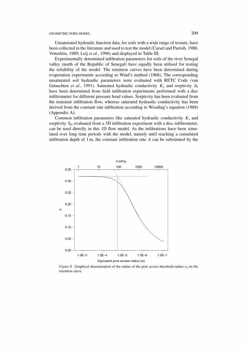
Figure 8. Graphical determination of the radius of the pore access threshold radius ra on theretention curve.

210C

.HA

MM

EC

KE

RE

TA

L.

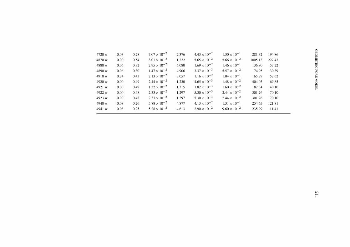
Table IV. Unsaturated hydraulic parameters from UNSODA data base (Leij et al., 1996), saturated conductivity, sorptivity andcorresponding pore radii R and Rret (determined on wetting branch of retention curve, and calculated with the proposed model)

Ref. θr θs α n Ks S0 R Rret

UNSODA cm−1 m s−1 m s−1/2 (×10−6 m) (×10−6 m)

1300 w 0.20 0.37 2.73 × 10−2 2.233 1.08 × 10−2 5.15 × 10−2 238.91 77.28

1310 w 0.27 0.33 2.02 × 10−2 3.273 6.41 × 10−3 1.97 × 10−2 308.53 48.50

1410 w 0.04 1.00 1.11 × 10−1 3.532 1.82 1.58 × 101 329.71 257.47

2020 w 0.50 0.71 1.87 × 10−1 1.383 9.18 × 10−1 3.13 × 10−1 2592.27 581.44

2021 w 0.58 0.65 5.39 × 10−2 2.258 1.35 × 10−1 1.51 × 10−1 1067.02 151.85

2022 w 0.53 0.71 3.21 × 10−1 1.409 2.85 5.28 × 10−1 3912.75 1003.93

2151 w 0.00 0.29 3.34 × 10−2 2.287 1.05 × 10−2 7.54 × 10−2 145.07 93.59

2310 w 0.05 0.30 5.01 × 10−2 7.979 4.49 × 10−2 1.89 × 10−1 226.06 90.93

3340 w 0.05 0.26 7.06 × 10−2 2.302 3.75 × 10−2 9.38 × 10−2 302.00 197.27

3341 w 0.00 0.37 4.83 × 10−2 1.280 1.26 × 10−2 1.99 × 10−2 552.64 143.87

4690 w 0.10 0.38 3.34 × 10−2 1.593 1.14 × 10−2 4.46 × 10−2 283.09 105.18

4700 w 0.00 0.39 2.76 × 10−2 1.628 8.52 × 10−3 6.00 × 10−2 183.87 86.67

4710 w 0.06 0.38 3.35 × 10−2 1.789 1.41 × 10−2 8.33 × 10−2 209.31 102.96

GE

OM

ET

RIC

POR

EM

OD

EL

211

4720 w 0.03 0.28 7.07 × 10−2 2.376 4.43 × 10−2 1.30 × 10−1 281.32 194.86

4870 w 0.00 0.54 8.01 × 10−2 1.222 5.65 × 10−2 5.66 × 10−2 1005.13 227.43

4880 w 0.06 0.32 2.95 × 10−2 6.080 1.69 × 10−2 1.46 × 10−1 136.80 57.22

4890 w 0.06 0.30 1.47 × 10−2 4.906 3.37 × 10−3 5.57 × 10−2 74.95 30.39

4910 w 0.24 0.43 2.13 × 10−2 3.057 1.16 × 10−2 1.04 × 10−1 165.79 52.62

4920 w 0.00 0.49 2.44 × 10−2 1.230 4.65 × 10−3 1.48 × 10−2 404.03 69.85

4921 w 0.00 0.49 1.32 × 10−2 1.315 1.82 × 10−3 1.60 × 10−2 182.34 40.10

4922 w 0.00 0.48 2.33 × 10−2 1.297 5.30 × 10−3 2.44 × 10−2 301.76 70.10

4923 w 0.00 0.48 2.33 × 10−2 1.297 5.30 × 10−3 2.44 × 10−2 301.76 70.10

4940 w 0.08 0.26 5.88 × 10−2 4.877 4.13 × 10−2 1.31 × 10−1 254.65 121.81

4941 w 0.08 0.25 5.28 × 10−2 4.613 2.90 × 10−2 9.60 × 10−2 235.99 111.41


saturated hydraulic conductivity Ks. The model describes the kinetic of wettingfront progression, hence experimental infiltration measurements have to be dividedby the corresponding saturated water content value (θs), in order to be compared tothe model. Consequently the corresponding infiltration parameters S/θs and A/θs

have been determined and introduced in Equations (18a) and (18b) in order tocalculate the pore access (ra) and pore radii (R). The pore size distribution foreach soil has been derived from its retention curve. A pore threshold radius (rret)considered as giving access to the chief part of the porous network in the soil, whichis equivalent to the air entry pressure, has been determined graphically with a curvetangent method (Figure 8) as described by Dullien (1979). As retention curves aremostly obtained during the drying phase (equivalent to a mercury intrusion formercury porosimetry), the corresponding pore size distribution are representativeof the pore access radii (ra). The direct determination of the pore radii (widenings)R, on coloured thin sections, has not been possible on the soils for which infiltrationexperiments have been performed. This information was also unavailable for thesoils selected from literature. Nevertheless the pore radius (R) can alternatively bederived from retention data for imbibition, considering the hysteresis is due to inkbottle geometry of pores. Despite being difficult to obtain, this kind of informa-tion is available in UNSODA database (Leij et al., 1996) for some soil samples(Table IV). However these wetting curves have usually only few points and fittingprocedure for determination of the unsaturated hydraulic parameters (θr, θr, α andn) was not very satisfactory. Nevertheless the same procedure as mentioned abovewas used to determine the pore radii on the wetting branch (imbibition) of theretention curve.

4. Results and Discussion

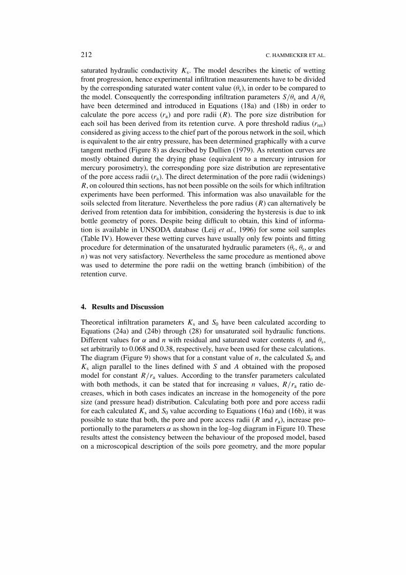
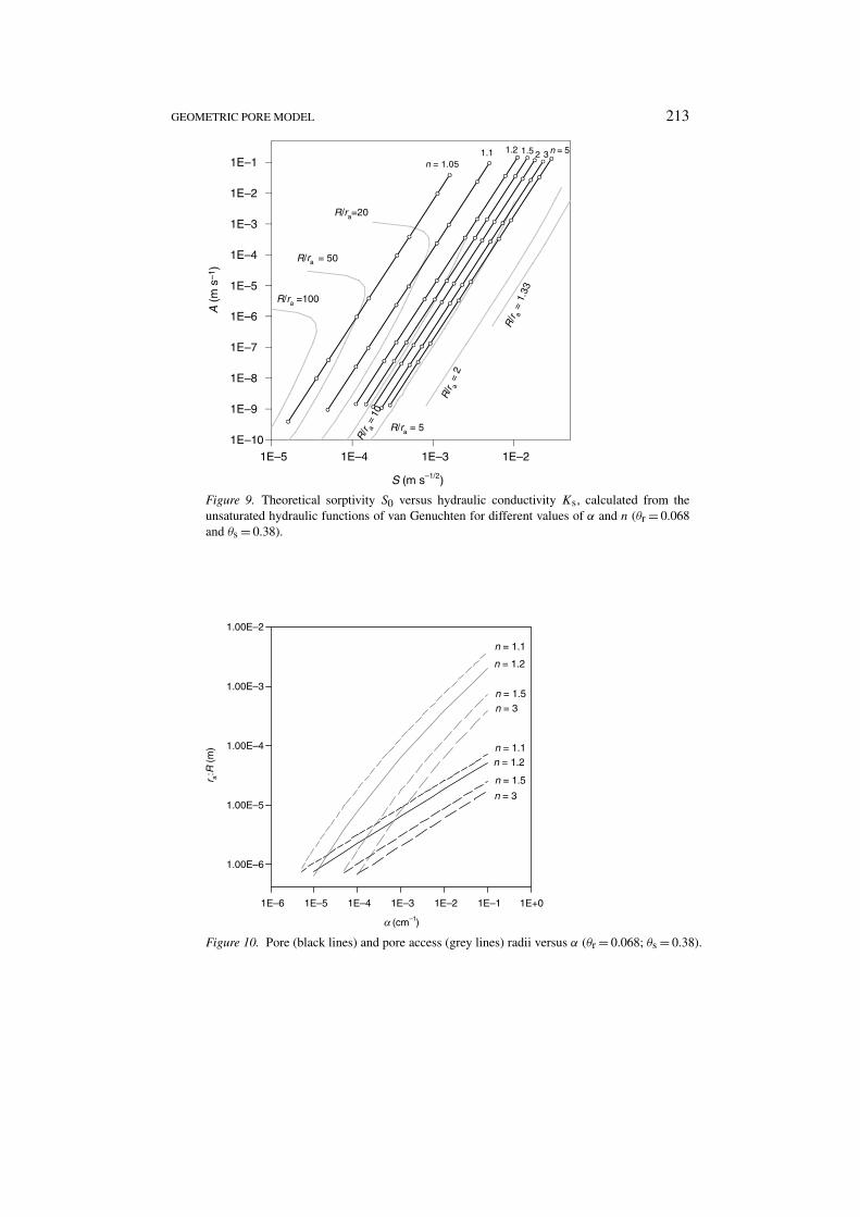
Theoretical infiltration parameters Ks and S0 have been calculated according toEquations (24a) and (24b) through (28) for unsaturated soil hydraulic functions.Different values for α and n with residual and saturated water contents θr and θs,set arbitrarily to 0.068 and 0.38, respectively, have been used for these calculations.The diagram (Figure 9) shows that for a constant value of n, the calculated S0 andKs align parallel to the lines defined with S and A obtained with the proposedmodel for constant R/ra values. According to the transfer parameters calculatedwith both methods, it can be stated that for increasing n values, R/ra ratio de-creases, which in both cases indicates an increase in the homogeneity of the poresize (and pressure head) distribution. Calculating both pore and pore access radiifor each calculated Ks and S0 value according to Equations (16a) and (16b), it waspossible to state that both, the pore and pore access radii (R and ra), increase pro-portionally to the parameters α as shown in the log–log diagram in Figure 10. Theseresults attest the consistency between the behaviour of the proposed model, basedon a microscopical description of the soils pore geometry, and the more popular


Figure 9. Theoretical sorptivity S0 versus hydraulic conductivity Ks, calculated from theunsaturated hydraulic functions of van Genuchten for different values of α and n (θr = 0.068and θs = 0.38).

Figure 10. Pore (black lines) and pore access (grey lines) radii versus α (θr = 0.068; θs = 0.38).


phenomenological models describing the unsaturated soil hydraulic parametersfrom which infiltration parameters have been derived or calculated with numericalresolution of the Richards’ equation.

As well as a theoretical validation, the model has been subjected to tests withexperimental data, on soils with textures ranging from silty clay to sand, of differentorigins. Table IV displays the unsaturated hydraulic functions data, the derivedparameters (S0, Ks, rret), and the corresponding pore and pore access radii (R, ra)calculated with the model.

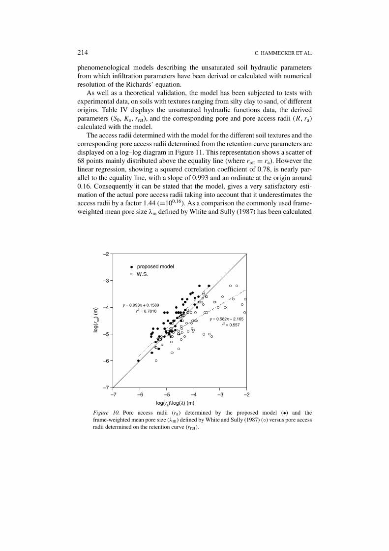
The access radii determined with the model for the different soil textures and thecorresponding pore access radii determined from the retention curve parameters aredisplayed on a log–log diagram in Figure 11. This representation shows a scatter of68 points mainly distributed above the equality line (where rret = ra). However thelinear regression, showing a squared correlation coefficient of 0.78, is nearly par-allel to the equality line, with a slope of 0.993 and an ordinate at the origin around0.16. Consequently it can be stated that the model, gives a very satisfactory esti-mation of the actual pore access radii taking into account that it underestimates theaccess radii by a factor 1.44 (=100.16). As a comparison the commonly used frame-weighted mean pore size λm defined by White and Sully (1987) has been calculated

Figure 10. Pore access radii (ra) determined by the proposed model (•) and theframe-weighted mean pore size (λm) defined by White and Sully (1987) (◦) versus pore accessradii determined on the retention curve (rret).


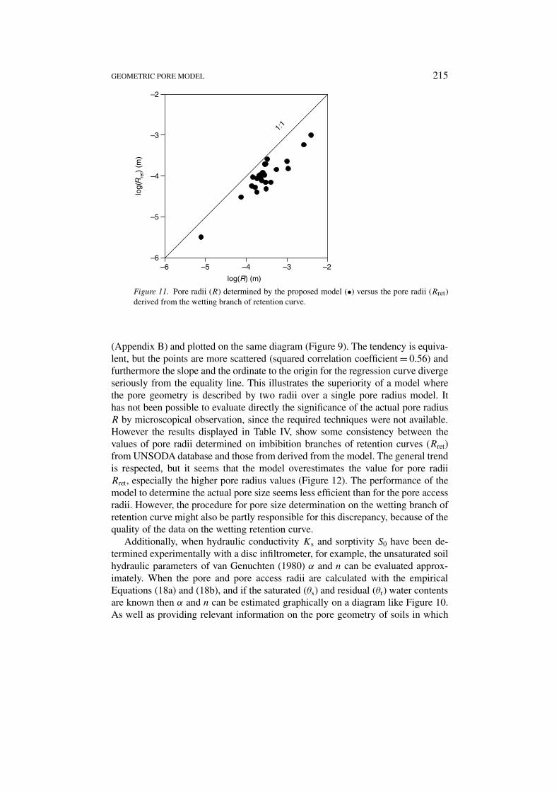
Figure 11. Pore radii (R) determined by the proposed model (•) versus the pore radii (Rret)derived from the wetting branch of retention curve.

(Appendix B) and plotted on the same diagram (Figure 9). The tendency is equiva-lent, but the points are more scattered (squared correlation coefficient = 0.56) andfurthermore the slope and the ordinate to the origin for the regression curve divergeseriously from the equality line. This illustrates the superiority of a model wherethe pore geometry is described by two radii over a single pore radius model. Ithas not been possible to evaluate directly the significance of the actual pore radiusR by microscopical observation, since the required techniques were not available.However the results displayed in Table IV, show some consistency between thevalues of pore radii determined on imbibition branches of retention curves (Rret)from UNSODA database and those from derived from the model. The general trendis respected, but it seems that the model overestimates the value for pore radiiRret, especially the higher pore radius values (Figure 12). The performance of themodel to determine the actual pore size seems less efficient than for the pore accessradii. However, the procedure for pore size determination on the wetting branch ofretention curve might also be partly responsible for this discrepancy, because of thequality of the data on the wetting retention curve.

Additionally, when hydraulic conductivity Ks and sorptivity S0 have been de-termined experimentally with a disc infiltrometer, for example, the unsaturated soilhydraulic parameters of van Genuchten (1980) α and n can be evaluated approx-imately. When the pore and pore access radii are calculated with the empiricalEquations (18a) and (18b), and if the saturated (θs) and residual (θr) water contentsare known then α and n can be estimated graphically on a diagram like Figure 10.As well as providing relevant information on the pore geometry of soils in which


Ks and S0 have been measured experimentally, this model also provides useful datafor estimating the unsaturated soil hydraulic parameters.

5. Conclusions

The aim of this paper is to present a geometrical model designed to provide quan-titative information on the size of pores involved in infiltration process in soils,derived from sorptivity and constant rate infiltration data. The model describes theinfiltration through a geometrical porous network composed of stacks of hollowspherical elements. It has been shown that the actual shape is an irrelevant factorfor infiltration, but that a varying radius along the infiltration front is determin-ing when proper infiltration kinetics are to be described. This model shows thatinfiltration is mainly governed by two geometrical parameters: the widening ofthe pores and the pore necks radii, each having a predominant influence, respec-tively, on the sorptivity and the constant gravity-driven infiltration rate. The Philipinfiltration parameters for limit conditions (when ra → R), determined with thismodel, have been compared to the results obtained by simple cylindrical modelsand thereby establish it’s numerical consistency. The microscopical pore model hasbeen tested theoretically with macroscpical unsaturated soil hydraulic functions.This test assesses the consistency of the proposed model according to the tradi-tional phenomenological models describing water transfer processes. An empiricalrelation between sorptivity, hydraulic conductivity, and the pore and pore accessradii has been defined for sorptivity values ranging from 10−6 to 10−1 m s−0.5 andhydraulic conductivity from 10−14 to 10−1 m s−1. Finally the model has been anal-ysed with soil data from literature and measured experimentally for a wide rangeof texture. The pore access radii calculated with the model have been comparedto the experimental pore access radii determined on the retention curve and foundto be in very good agreement despite being underestimated by an average factorof 1.44. In comparison the frame-weighted mean pore size λm (White and Sully,1987) also calculated with sorptivity and hydraulic conductivity, does not accord aswell with experimental pore access radii. This demonstrates that a pore model withtwo radii (throat and widening) is more suitable to describe infiltration processes insoils than a single pore radius model. Although actual observation of the pore sizewas not possible, these data were derived from imbibition retention curves (Rret)

and compared to the widening radii (R) of the model. The results are consistent asthey follow the same general trend, but the pore radii (R) obtained with the modelare systematically superior to those obtained on retention curves (Rret). However,this relative discrepancy cannot only be attributed to the model because of the poorquality of data for imbibition retention curves.

This model can also be used in the estimation of α and n when Ks and S0 havebeen measured experimentally. Finally it can be stated that the introduction of asecond pore radius in this simple model improves notably the relation between themicroscopical description of pore size and macroscopical infiltration processes.


Acknowledgements

This work was partially supported by the EC-project FED and the regional pole forresearch on sudano-sahelian irrigated systems (PSI). The authors would also liketo thank Dr Michel Vauclin (LTHE, Grenoble) and Dr Laurent Bruckler (INRA,Avignon) for their useful advise and comments on this paper.

Appendix A.

Hydraulic conductivity measured with a tension disc infiltrometer has been calcu-lated according to Wooding’s equation (1968):

q0 = K0 + 4.0

π + rd(A.1)

.0 =∫ h0

hi

K(h) dh (A.2)

where rd is the disk diameter, q0 is the constant infiltration rate (A), K0 is the hy-draulic conductivity, and .0 is the matric flux potential. hi and h0 are, respectively,the initial and applied pressure heads.

Assuming an exponential relation for conductivity with pressure head (Gardner,1958): K(h) = Ks exp(α1h), Equation (A.1) simplifies to:

q0 = Ks exp(α1h0)

(1 + 4

α1πrd

)(A.3)

As sorptivity S0 is defined for an initial dry soil, it has been determined duringthe first stage of infiltration, according to Philip’s equation (1957), and assuming arelation between initial water content θi and the measured sorptivity S (Musy andSoutter, 1991):

S0 = S

(1 − θi

θs

)−1

(A.4)

Appendix B.

White and Sully (1987) defined a now commonly used frame-weighted mean poresize for given infiltration parameters:

λm = σ (θ0 − θn)K0

ρgbS20

(B.1)

where σ is the surface tension of water (7.2 × 10−2 N s m−2), ρ is the density ofwater (1000 kg m−3), g is the gravitational constant (9.81 m s−1), θn and θ0 are the


initial volumetric water content and the water content at an imposed water pressurehead, K0 is the hydraulic conductivity for this pressure head, which in this case canbe assimilated to A, S0 is the corresponding sorptivity and b a constant usually setat 0.55 (White and Sully, 1987; Warrick and Broadbridge, 1992; Angulo-Jaramilloet al., 1997).

References

Angulo-Jaramillo, R., Moreno, F., Clothier, B. E., Thony, J. L., Vachaud, G., Fernandez-Boy, E. andCayuela, J. A.: 1997, Seasonal variation of hydraulic properties of soils measured using a tensiondisk infiltrometer, Soil. Sci. Soc. Am. J. 61, 27–32.

Brooks, R. H. and Corey, A. T.: 1966, Properties of porous media affecting fluid flow, J. Irr. Drain.Div., Am. Soc. Civ. Eng. 96, 2535–2548.

Case, C. M.: 1990, Rate of rise of liquid in capillary tube-revisited, Am. J. Phys. 58, 888–889.Case, C. M.: 1994, Physical Principles of Flow in Unsaturated Porous Media, Oxford University

Press, New York, 374 pp.Carsel, R. F. and Parrish, R. S.: 1988, Developing joint probability distributions of soil water retention

characteristics, Water Resour. Res. 24, 755–759.Chavetau, G.: 1965, Essai sur la loi de Darcy et les ecoulements laminaires a perte de charge non-

lineaire, These Docteur-Ingenieur de l’Universite de Toulouse.Dullien, F. A. L.: 1979, Porous Media: Fluid Transport and Pore Structure, Academic Press,

New York, 396 pp.Dullien, F. A. L., El-Sayed, M. S. and Batra, V. K.: 1977, Rate of capillary rise in porous media with

non uniform pores, J. Colloids Interf. Sci. 60, 497–506.FAO, ISRIC and ISSS: 1994, Draft World Reference Base for Soil Resources, Wageningen.Green, W. H. and Ampt, G. A.: 1911, Studies in soil physics. I. Flow of air and water through soils,

J. Agric. Sci. 4, 1–24.Grismer, M. E.: 1986, Pore size distribution and infiltration, Soil Sci. 14, 249–260.Hammecker, C. and Jeannette, D.: 1994, Modelling the capillary imbibition kinetics in sedimentary

rocks: role of petrographical features, Transp. Porous Media 17, 285–303.Hammecker, C., Mertz, J. D., Fischer, C. and Jeannette, D.: 1993, A geometrical model for numerical

simulation of capillary imbibition in sedimentary rocks, Transp. Porous Media 12, 125–141.Hillel, D.: 1998, Environmental Soil Physics, Academic Press, San Diego, 771 pp.Kusakov, M. M. and Nekrasov, D. N.: 1966, Capillary hysteresis in the rise of wetting liquids

in single capillaries and porous bodies, in: B.V. Deryagin (ed.), Research in Surface Forces,New York, pp. 193–202.

Leij, F. J., Alves, W. J., van Genuchten, M. T. and Williams, J. R.: 1996, The UNSODA UnsaturatedSoil Hydraulic Database. United States Environmental Agency document EPA/600/R-96/095,103 pp.

Levine, S., Lowndes, J. and Reed, P.: 1980, Two phase fluid flow and hysteresis in a periodic capillarytube, J. Colloid Interf. Sci. 77, 253–263.

Marmur, A.: 1989, Capillary rise and hysteresis in periodic porous media, J. Colloid Interf. Sci. 127,362–372.

Marshall, T. J.: 1958, A relation between permeability and size distribution of pores, J Soil. Sci. 9,1–8.

Mualem, Y.: 1976, A new model for predicting the hydraulic conductivity of unsaturated porousmedia, Water Resour. Res. 12, 513–522.

Musy, A. and Soutter, M.: 1991, Physique du sol. Presses Polytechniques et universitaires romandes(ed.), Lausanne, Switzerland.


Parlange, J. Y.: 1975, On solving the flow equation in unsaturated soils by optimization: Horizontalinfiltration, Soil Sci. Soc. Am. Proc. 39, 415–418.

Peiris, M. G. C. and Tenakone, K.: 1980, Rate of rise of liquid in a capillary tube, Am. J. Phys. 48,415.

Perroux, K. M. and White, I.: 1988, Design for disc permeameters, Soil. Sci. Soc. Am. J. 52,1205–1215.

Philip, J. R.: 1957, Theory of infiltration. 4. Sorptivity and algebraic infiltration equations, Soil Sci.84, 257–264.

Reynolds, W. D. and Elrick, D. E.: 1991, Determination of hydraulic conductivity using a tensioninfiltrometer, Soil. Sci. Soc. Am. J. 55, 633–639.

Richards, L. A.: 1931, Capillary conduction of liquids in porous medias, Physics 1, 318–333.Smettem, K. R. J. and Clothier, B. E.: 1989, Measuring unsaturated sorptivity and hydraulic

conductivity using multiple disc permeameters, J. Soil Sci. 40, 563–568.Thony, J. L., Vachaud, G., Clothier, B. E. and Angulo-Jaramillo, R.: 1991, Field measurements of

the hydraulic properties of soil, Soil Tech. 4, 111–123.van Brakel, J.: 1975, Pore space models for transport phenomena in porous media. Review and

evaluation with special emphasis on capillary transport, Powder Technol. 11, 205–236.van Genuchten, M. Th.: 1980, A closed form equation for predicting the hydraulic conductivity of

unsaturated soils, Soil Sci. Soc. Am. J. 44, 892–898.van Genuchten. M. Th., Leij, F. J. and Yates, S. R.: 1991, The RETC code for quantifying the

hydraulic functions of unsaturated soils, US Salinity Laboratory, US Dep. of Agric. Res. Serv.,Riverside, CA.

Vetterlein, E.: 1989, Bodenphysikalische Kennwerte fur Substrat-Horizont-Gruppen, in: V. Koepke(ed.), Bodenwasserregulierung, Muncheberg, Germany.

Warrick, A. W. and Broadbridge, P.: 1992, Sorptivity and macroscopic capillary length relationships,Water Resour. Res. 28, 427–431.

Washburn, E. W.: 1921, The dynamics of capillary flow, Phys. Rev. 17, 273–283.Wind, G. P.: 1968, Capillary conductivity data estimated by a simple method, in: P. E. Rijtema and

H. Wassink (eds), Water in the Unsaturated Zone, Proc. of the Wageningen Symposium, June1966, IASH Gentbrugge/UNESCO Paris, Vol. 1, pp. 181–191.

White, I. and Sully, M. J.: 1987, Macroscopic and microscopic capillary length and times scales fromfield infiltration, Water Resour. Res. 23, 1514–1522.

Wooding, R. A.: 1968, Steady infiltration from a shallow circular pond, Water Resour. Res. 4,1259–1273.

a geometrical pore model for estimating the microscopical pore geometry of soil with infiltration...

Documents