a genetic algorithm for facility layout design in flexible ... · pdf filea genetic algorithm...

A Genetic Algorithm For Facility Layout Design

In Flexible Manufacturing Systems

Maheswaran Rajasekharan

Brett A. Peters

Taho Yang

Submitted February 7, 1996

Revised December 19, 1996

This working paper is not to be copied, quoted, or cited without the permission of the

authors. Address correspondence to Brett A. Peters, Dept. of Industrial Engineering,

Texas A&M University, College Station, TX 77843–3131 or email to [email protected]

A Genetic Algorithm For Facility Layout Design In

Flexible Manufacturing Systems

Abstract

The flexible manufacturing system (FMS) facility layout problem (FLP) involves the positioning of cells

within a given area so as to minimize the material flow costs between cells. The FLP design includes

specifying the spatial coordinates of each cell, the orientation of each cell in either a horizontal or vertical

position, and the position of each cell’s pickup and dropoff points. The layout design problem is both

tactically and strategically important since the layout plays a large role in determining the efficiency and

flexibility of the system. The FMS layout problem differs from traditional layout problems in that there are

additional constraints on a cell’s shape and orientation and the location of the pickup/dropoff points must

be determined. A mixed integer programming formulation for the FLP developed by Das (1993) is adapted

and heuristically solved in this paper. Because of the NP-hard nature of the solution space, a genetic

algorithm based decomposition strategy is proposed and computationally tested. A comparison of the

computational results with the existing methods indicate that the heuristic is a viable alternative for

efficiently and effectively generating layout designs for flexible manufacturing systems.

1

A Genetic Algorithm For Facility Layout Design In

Flexible Manufacturing Systems

1. Introduction

Flexible manufacturing systems (FMSs) have emerged in recent years as a viable answer to meet the

market demand for increased product variety, short product life cycles, and uncertain demand. From a

strategic perspective, an efficient layout design is critical for the implementation of an FMS, since the

layout is difficult to design, costly to modify, and significantly affects the efficiency of the entire system.

It has been estimated that 20%-50% of the total operating expenses within manufacturing operations are

attributed to material handling, and it has been reported that effective layout design will reduce these

costs by at least 10%-30% (Tompkins and White, 1984). In addition to material handling costs, the

facility layout also impacts the production costs and the work-in-process inventory levels.

The design problem in a flexible manufacturing system consists of three distinct stages: (i) selection and

grouping of production and material handling equipment into cells, (ii) allocation of the machine cells to

areas within the shop-floor (facility layout), and (iii) detailed layout of the machines within each cell

(machine layout). The first problem in this design hierarchy, the cell grouping problem has been considered

by numerous researchers in the past, and is not considered in this paper. This paper addresses the FMS

facility layout problem (FLP) by assuming that the composition of each cell is known. The detailed

machine layout within a cell can be determined using the same approach presented here by adjusting the

level of detail to consider each cell as a separate layout problem.

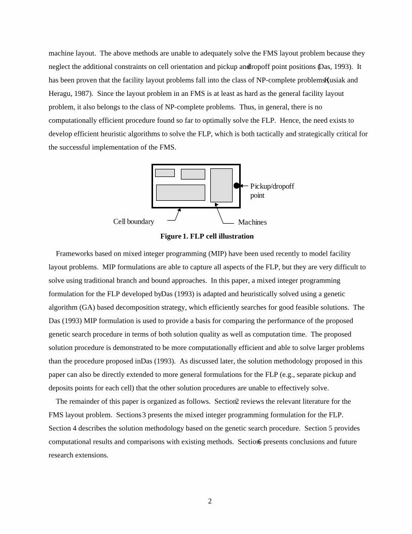
The layout problem in an FMS differs from the traditional facility layout problem in that there are

additional features that require explicit modeling. The cells in an FMS can be represented by rectangular

blocks. The pickup/dropoff point positions of each cell are usually located on either one of the cell axes.

(Das, 1993). In this paper, it is assumed that the pickup/dropoff positions are collocated and are restricted

to be on either one of the cell axes. Hence an FLP design includes specifying the spatial coordinates of

each cell, the orientation of each cell in either a horizontal or vertical position, and the positions of each

cell’s pickup and dropoff point. Figure 1 illustrates the conceptual configuration of a cell.

The general facilities layout problem considers the area of the cells, but not the shape, and has been

modeled in the past in several ways, such as a quadratic assignment problem (QAP), a quadratic set

covering problem (QSCP), a linear integer programming problem, and a graph theoretic problem (Kusiak

and Heragu, 1987). In contrast, the general machine layout problem (MLP) also considers the cell

geometry, and QAP and other integer programming formulations have been suggested for determining the

2

machine layout. The above methods are unable to adequately solve the FMS layout problem because they

neglect the additional constraints on cell orientation and pickup and dropoff point positions (Das, 1993). It

has been proven that the facility layout problems fall into the class of NP-complete problems (Kusiak and

Heragu, 1987). Since the layout problem in an FMS is at least as hard as the general facility layout

problem, it also belongs to the class of NP-complete problems. Thus, in general, there is no

computationally efficient procedure found so far to optimally solve the FLP. Hence, the need exists to

develop efficient heuristic algorithms to solve the FLP, which is both tactically and strategically critical for

the successful implementation of the FMS.

Figure 1. FLP cell illustration

Frameworks based on mixed integer programming (MIP) have been used recently to model facility

layout problems. MIP formulations are able to capture all aspects of the FLP, but they are very difficult to

solve using traditional branch and bound approaches. In this paper, a mixed integer programming

formulation for the FLP developed by Das (1993) is adapted and heuristically solved using a genetic

algorithm (GA) based decomposition strategy, which efficiently searches for good feasible solutions. The

Das (1993) MIP formulation is used to provide a basis for comparing the performance of the proposed

genetic search procedure in terms of both solution quality as well as computation time. The proposed

solution procedure is demonstrated to be more computationally efficient and able to solve larger problems

than the procedure proposed in Das (1993). As discussed later, the solution methodology proposed in this

paper can also be directly extended to more general formulations for the FLP (e.g., separate pickup and

deposits points for each cell) that the other solution procedures are unable to effectively solve.

The remainder of this paper is organized as follows. Section 2 reviews the relevant literature for the

FMS layout problem. Sections 3 presents the mixed integer programming formulation for the FLP.

Section 4 describes the solution methodology based on the genetic search procedure. Section 5 provides

computational results and comparisons with existing methods. Section 6 presents conclusions and future

research extensions.

Pickup/dropoffpoint

Cell boundary Machines

3

2. Literature Survey

The first FMS design step is to group the machines into cells. This step can be done in a variety of ways

including group technology based algorithms such as those by Lee and Garcia-Diaz (1993) or Chan and

Milner (1982).

Various techniques can be used to determine the layout of each cell depending on the characteristics of

the particular problem. In general, the machine sizes are such that the pickup and dropoff points can be

assumed to be located at the cell centroid. In fact, the solution procedure for the FLP can also apply to the

machine layout design problem in an FMS cell, since the machine layout design problem is a micro-version

of the FMS layout design problem. Heragu and Kusiak (1988 and 1990) contain more specific information

about the machine layout problem.

This paper assumes that the machine arrangement inside a cell has been previously determined; thus, a

cell geometry as well as the distance between the potential pickup/dropoff positions and the cell centroid

are known. The FLP arranges the FMS cells on an open-field floor space in order to minimize the total

material handling costs.

Traditional layout design problems have been extensively studied, but these procedures are unable to

solve the FLP because of the insufficient design information on a cell’s shape and pickup/dropoff point

positions. For a detailed discussion of traditional layout approaches, readers are referred to Francis et al.

(1992), Kusiak and Heragu (1987), and Meller and Gau (1996).

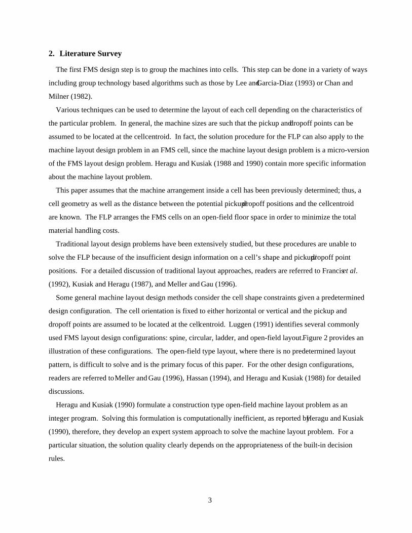
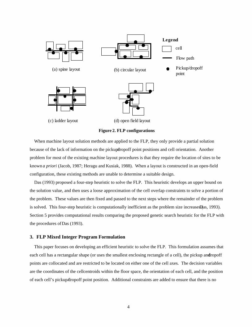
Some general machine layout design methods consider the cell shape constraints given a predetermined

design configuration. The cell orientation is fixed to either horizontal or vertical and the pickup and

dropoff points are assumed to be located at the cell centroid. Luggen (1991) identifies several commonly

used FMS layout design configurations: spine, circular, ladder, and open-field layout. Figure 2 provides an

illustration of these configurations. The open-field type layout, where there is no predetermined layout

pattern, is difficult to solve and is the primary focus of this paper. For the other design configurations,

readers are referred to Meller and Gau (1996), Hassan (1994), and Heragu and Kusiak (1988) for detailed

discussions.

Heragu and Kusiak (1990) formulate a construction type open-field machine layout problem as an

integer program. Solving this formulation is computationally inefficient, as reported by Heragu and Kusiak

(1990), therefore, they develop an expert system approach to solve the machine layout problem. For a

particular situation, the solution quality clearly depends on the appropriateness of the built-in decision

rules.

4

Figure 2. FLP configurations

When machine layout solution methods are applied to the FLP, they only provide a partial solution

because of the lack of information on the pickup/dropoff point positions and cell orientation. Another

problem for most of the existing machine layout procedures is that they require the location of sites to be

known a priori (Jacob, 1987; Heragu and Kusiak, 1988). When a layout is constructed in an open-field

configuration, these existing methods are unable to determine a suitable design.

Das (1993) proposed a four-step heuristic to solve the FLP. This heuristic develops an upper bound on

the solution value, and then uses a loose approximation of the cell overlap constraints to solve a portion of

the problem. These values are then fixed and passed to the next steps where the remainder of the problem

is solved. This four-step heuristic is computationally inefficient as the problem size increases (Das, 1993).

Section 5 provides computational results comparing the proposed genetic search heuristic for the FLP with

the procedures of Das (1993).

3. FLP Mixed Integer Program Formulation

This paper focuses on developing an efficient heuristic to solve the FLP. This formulation assumes that

each cell has a rectangular shape (or uses the smallest enclosing rectangle of a cell), the pickup and dropoff

points are collocated and are restricted to be located on either one of the cell axes. The decision variables

are the coordinates of the cell centroids within the floor space, the orientation of each cell, and the position

of each cell’s pickup/dropoff point position. Additional constraints are added to ensure that there is no

cell

Flow path

Legend

(c) ladder layout

(b) circular layout

(d) open field layout

(a) spine layout Pickup/dropoffpoint

5

overlap between cells. The distance between cell pickup and deposit points is estimated with a rectilinear

distance metric. The absolute value signs are removed by using additional variables and constraints.

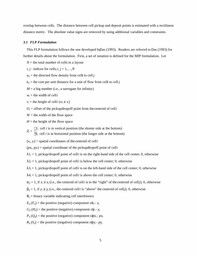
3.1 FLP Formulation

This FLP formulation follows the one developed by Das (1993). Readers are referred to Das (1993) for

further details about the formulation. First, a set of notation is defined for the MIP formulation. Let

N = the total number of cells in a layout

i, j : indices for cells; i, j = 1,…,N

uij = the directed flow density from cell i to cell j

εij = the cost per unit distance for a unit of flow from cell i to cell j

M = a big number (i.e., a surrogate for infinity)

wi = the width of cell i

vi = the height of cell i (wi ≥ vi)

Oi = offset of the pickup/dropoff point from the centroid of cell i

W = the width of the floor space

H = the height of the floor space

Zi = 1, cell is in vertical position (the shorter side at the bottom)

0, cell is in horizontal position (the longer side at the bottom)

i

i

(xi, yi) = spatial coordinates of the centroid of cell i

(pxi, pyi) = spatial coordinate of the pickup/dropoff point of cell i

λ1i = 1, pickup/dropoff point of cell i is on the right-hand side of the cell center; 0, otherwise

λ2i = 1, pickup/dropoff point of cell i is below the cell center; 0, otherwise

λ3i = 1, pickup/dropoff point of cell i is on the left-hand side of the cell center; 0, otherwise

λ4i = 1, pickup/dropoff point of cell i is above the cell center; 0, otherwise

α ij = 1, if xi ≥ xj (i.e., the centroid of cell i is to the “right” of the centroid of cell j); 0, otherwise

βij = 1, if yi ≥ yj (i.e., the centroid cell i is “above” the centroid of cell j); 0, otherwise

θij = binary variable indicating cell interference

Eij (Fij) = the positive (negative) component of xi - xj

Gij (Hij) = the positive (negative) component of yi - yj

Pij (Qij) = the positive (negative) component of pxi - pxj

Rij (Sij) = the positive (negative) component of pyi - pyj

6

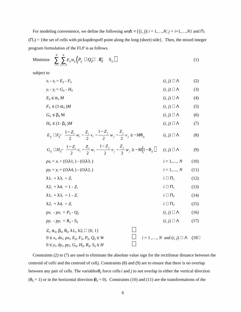
For modeling convenience, we define the following sets: Λ = {( i, j)| i = 1,…,N; j = i+1,…,N} and Π1

(Π2) = {the set of cells with pickup/dropoff point along the long (short) side}. Then, the mixed integer

program formulation of the FLP is as follows.

Minimize ( )ε ij ijj i

N

i

N

ij ij ij iju P Q R S= +=∑∑ + + +

11

(1)

subject to

xi - xj = Eij - Fij (i, j) ∈ Λ (2)

yi - yj = Gij - Hij (i, j) ∈ Λ (3)

Eij ≤ α ij M (i, j) ∈ Λ (4)

Fij ≤ (1-α ij )M (i, j) ∈ Λ (5)

Gij ≤ βij M (i, j) ∈ Λ (6)

Hij ≤ (1- βij )M (i, j) ∈ Λ (7)

E FZ

wZ

vZ

wZ

v Mij iji

ii

ij

jj

j ij+ −−

− −−

− ≥ −1

2 2

1

2 2θ (i, j) ∈ Λ (8)

( )G HZ

vZ

wZ

vZ

w Mij iji

ii

ij

jj

j ij+ −−

− −−

− ≥ − −1

2 2

1

2 21 θ (i, j) ∈ Λ (9)

pxi = xi + (Oiλ1i ) - (Oiλ3i ) i = 1,...., N (10)

pyi = yi + (Oiλ4i ) - (Oiλ2i ) i = 1,...., N (11)

λ1i + λ3i = Zi i ∈ Π1 (12)

λ2i + λ4i = 1 - Zi i ∈ Π1 (13)

λ1i + λ3i = 1 - Zi i ∈ Π2 (14)

λ2i + λ4i = Zi i ∈ Π2 (15)

pxi - pxi = Pij - Qij (i, j) ∈ Λ (16)

pyi - pyi = Rij - Sij (i, j) ∈ Λ (17)

Zi, α ij, βij, θij, λ1i, λ2i ∈ {0, 1} 0 ≤ xi, dxi, pxi, Eij, Fij, Pij, Qij ≤ W i = 1 ,…, N and (i, j) ∈ Λ (18)

0 ≤ yi, dyi, pyi, Gij, Hij, Rij, Sij ≤ H Constraints (2) to (7) are used to eliminate the absolute value sign for the rectilinear distance between the

centroid of cell i and the centroid of cell j. Constraints (8) and (9) are to ensure that there is no overlap

between any pair of cells. The variables θij force cells i and j to not overlap in either the vertical direction

(θij = 1) or in the horizontal direction (θij = 0). Constraints (10) and (11) are the transformations of the

7

rectilinear distances between the pickup/dropoff point of cell i and its centroid. Constraints (12) to (15)

relate a cell’s pickup/dropoff point position to its cell centroid for the different configurations. Constraints

(16) and (17) are used to remove the absolute value signs of the distance between the pickup/dropoff point

of cell i and the pickup/dropoff point of cell j. Constraints (18) specify the bounds for each variable. Due

to the interrelationships between pickup/dropoff points, λ3i and λ4i are not required to be integer restricted.

4. Solution Methodology

The formulation presented in Section 3 has 1.5(N2 − N) binary variables for a layout problem of N cells

and is very hard to solve for realistic problems using standard linear programming based branch and bound

approaches. In this paper, a two step hierarchical decomposition approach is developed to intelligently

search the solution space to obtain good solutions in a fast manner. The first step in the hierarchy is to

determine the spatial sequence for cells in both x (horizontal) and y (vertical) directions. This step restricts

the candidate region for a cell’s location in an open-field floor space. A greedy genetic algorithm is

developed to determine the spatial sequence for the cells, which defines the candidate regions. The second

step in the hierarchy is to search this restricted space to obtain a good solution to the FMS layout problem.

A slightly different genetic search procedure is developed to search the restricted solution space. Figure 3

illustrates this two-step GA based heuristic procedure for solving the FLP.

Figure 3. GA based two-step heuristic procedure

Input information• Flow density matrix• Cell geometry• Distance between the

pickup/dropoff position andcentroid for each cell

Output layout design• Cell centroid coordinates• Cell orientations• P/D point positions

Layout evaluation

Step 1: Greedy geneticprocedure for spatial sequence

determinationGenerate reduced FLPformulation based on bestspatial relative positioningfrom search procedure

Step 2: GA procedure for FLPSolve the reduced FLPformulation

GA procedure

8

4.1 Overview of Genetic Algorithms

Genetic algorithms attempt to mimic the biological evolution process for discovering good solutions.

They are based on a direct analogy to Darwinian natural selection and mutations in biological reproduction

and belong to a category of heuristics known as randomized heuristics that employ randomized choice

operators in their search strategy and do not depend on complete a priori knowledge of the features of the

domain. These operators have been conceived through abstractions of natural genetic mechanisms such as

crossover and mutation and have been cast into algorithmic forms (Arunkumar and Chockalingam, 1993).

Repetitive executions of these heuristics need not yield the same solution.

A genetic algorithm maintains a collection or population of solutions throughout the search. It initializes

the population with a pool of potential solutions to the problem and seeks to produce better solutions

(individuals) by combining the better of the existing ones through the use of one or more genetic operators.

Individuals are chosen at each iteration with a bias towards those with the best objective values. With

various mapping techniques and an appropriate measure of fitness of individuals (i.e., objective function

value), a genetic algorithm can be tailored to evolve a solution for many types of problems, including

optimization of a function or determination of the proper order of a sequence.

Theoretical analyses suggest that genetic algorithms can quickly locate high performance regions in

extremely large and complex search spaces. In addition, the distributed and repeated sampling can lead to

some natural insensitivity to noisy feedback. The genetic algorithm based heuristics are highly suited for

application to large instances of problems that are hard to model and for which no satisfactory tailored

algorithms are available. Readers are referred to Schaffer et al. (1992), Goldberg (1989), and Holland

(1992) for more information about genetic algorithms.

For large MIP formulations, stochastic global optimization methods such as simulated annealing (SA)

and genetic algorithms have recently shown great promise. The SA based approaches operate on one

intermediate solution at a time, whereas GA utilizes the past information by simultaneously operating on a

population of solutions. Genetic algorithms can combine the desirable features of two radically different

previous solutions unlike the SA approach where only one previous solution is transmitted (Banerjee et al.,

1994). Researchers in the past have successfully applied genetic approaches for facilities layout design. In

particular, Banerjee et al. (1992) and Banerjee and Zhou (1995) have successfully used a genetic approach

to determine the facilities layout design for a single loop material flow path configuration.

4.2 Basic Genetic Algorithm Procedure

The search technique consists of generating an initial population of strings (symbolic representation of a

set of solutions using binary bits) at random. Each solution is assigned a numerical evaluation of its fitness

9

by an objective function, which is a mathematical function that maps a particular solution onto a single

positive number that is a measure of the solution’s worth. During each iteration (generation), each

individual string in the current population is evaluated using this measure of fitness. New strings (children)

for the next generation are selected from the current population of strings (parents) by a process known as

selection. A random selection process is used with a higher probability given for strings with higher fitness

values. Such a selection scheme systematically eliminates low-fitness individuals from the population from

one generation to the next. New generations can be produced either synchronously, so that the old

generation is completely replaced, or asynchronously, so that the generations overlap. This paper uses the

technique of steady-state reproduction without duplicates proposed by Whitley (1988) and Syswerda

(1989). This technique creates a certain number of children to replace the parents in the population, but

discards children that are duplicates of current individuals in the population.

Two genetic operators, crossover and mutation, are probabilistically applied to create a new population

of individuals. In crossover, individual strings in the current population are randomly selected two at a

time as parents, and the crossover operation exchanges cross sections of the parents to generate two new

individuals. A cut point is randomly chosen within the breeding pair of parent strings. New individuals are

formed by combining the initial components of the first parent string with the last components of the second

parent string and vice versa. The number of crossovers done in a generation is controlled by the crossover

rate (CR), which is defined as the ratio of the number of new individuals produced in each generation (by

crossover) to the population size. Mutation involves flipping a 0 bit to 1 or vice versa. The number of

bits to mutate and the specific bits to mutate are chosen in a random manner. The number of mutations

performed in a generation is controlled by a mutation rate parameter (MR), which is defined as the ratio of

the new individuals produced in each generation (by mutation) to the population size.

In the GA based solution procedure, the number of new individuals created at each iteration is (CR +

MR)P = δP. The remaining individuals are obtained by deterministically copying the individuals with the

top (1-δ)100% fitness from the previous generation. Parent individuals are selected as candidates for

crossover or mutation using the following selection process. An individual is selected at random and its

objective function value is compared with the average objective function value of the generation. If it has a

better objective function value than the generation average, it is accepted as a parent. If its objective

function value is lower than the generation average, it is accepted as a parent with probability γ < 1.

Genetic algorithms are domain independent because they require no explicit notion of a neighborhood.

Hence, crossover and mutation may not always produce feasible solutions. Therefore, the feasibility of a

newly created individual is ascertained before inserting it in the population to replace a parent string.

10

4.3 Genetic Algorithm Based Two Step Heuristic Procedure

The overall design of the specific genetic search procedure developed for solving the FLP is depicted in

Figure 4. The details of the two steps in the heuristic procedure are presented in Sections 4.3.1 and 4.3.2.

Input Parameters

Start

Generate a feasible spatialsequence for the cells at random

Yes

No

Yes

Generate at random values forthe cell interference variables

Yes

No

Yes

No

Population of strings

Crossover andMutation

Selection

Yes

No

Solve reduced FLP formulation byBranch & Bound procedure for layout

fitness determination

No

CREATION OF NEXTGENERATION

Yes

Obtain best result anddraw layout

GENETIC ALGORITHM FOR FLP

Is stringduplicated ?

Is population sizereached ?

No



Stop rulesreached ?

Population of strings

Crossover andMutation

Selection

Obtain best spatialsequence

Yes

No


GENETIC ALGORITHM FORSPATIAL SEQUENCEDETERMINATION

Is population sizereached ?

End





Figure 4. Genetic algorithm search procedure for FLP

11

4.3.1 Genetic Algorithm for Spatial Sequence Determination

The first step in the heuristic procedure for solving the FLP is to determine the relative spatial

positioning among the cells. A greedy genetic algorithm has been developed to determine the spatial

sequence for the cells in an open-field floor space. The algorithm performs a first search with no

backtracking and hence the term “greedy” is used. The string for the genetic algorithm is in binary code

and is of size 1.5(N2 − N) for a layout problem of N cells. The first 0.5(N2 − N) bits in the string represent

the spatial sequence for the cells in the x (horizontal) direction corresponding to the variables α ij in the

formulation. The second 0.5(N2 − N) bits in the string represent the spatial sequence for the cells in the y

(vertical) direction corresponding to the variables βij in the formulation. The third 0.5(N2 − N) bits in the

string represent the cell interference information corresponding to the variables θij in the formulation.

A feasible spatial sequence can be obtained by randomly generating unique values for xi’s and yi’s and

ranking them according to these values. From these ordered xi’s and yi’s, the values for the α ij and βij

variables can be determined (recall that α ij (βij) = 1 if xi ≥ xj (yi ≥ yj)). This process provides the values for

the first (N2 − N) values of the string. For the cell interference variables (θij), a one in the string means that

cell i and cell j will not overlap in the y (vertical) direction, and a zero in the string means that there will be

no overlap in the x (horizontal) direction. The values for these variables are generated at random. A given

string thus fixes the α ij, βij, and θij variables in the formulation. The resulting reduced formulation can be

easily solved using a branch and bound procedure to determine the best layout given the restrictions

specified by the string. The resulting material handling cost (objective value) for the cell layout specified

by that particular string is considered as the measure of the string’s fitness or competence.

The genetic algorithm procedure can be summarized as follows:

Initialize a population of feasible solutions

1. Generate at random a feasible spatial sequence for the cells (α ij and βij) and values for the cell

interference variables (θij).

2. Repeat step 1 until P feasible solutions are obtained.

Evaluate each individual in the population

3. Based on the α ij, βij, and θij values determine the objective function value for each individual in the

population using the branch and bound procedure. This step creates a specific layout that satisfies

the relative position of cells specified by α ij, βij, and θij. The material handling cost of this layout is

used as the objective function value for the individual.

Create new individuals using genetic operators

12

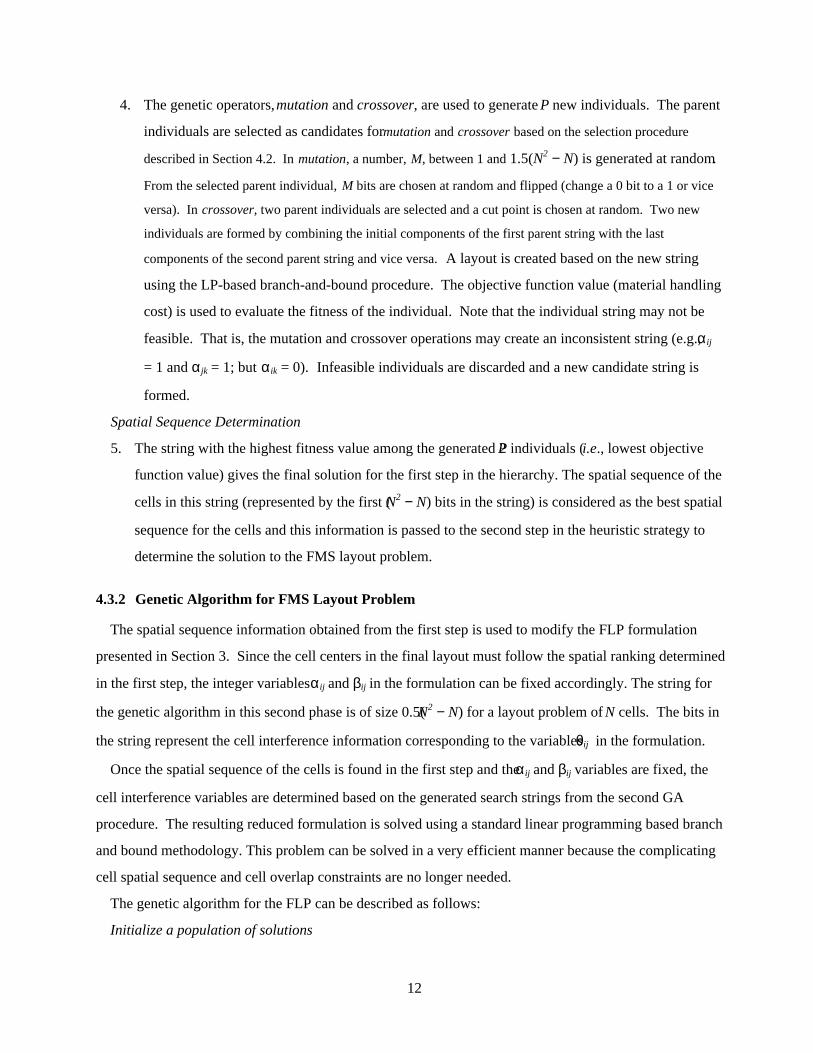
4. The genetic operators, mutation and crossover, are used to generate P new individuals. The parent

individuals are selected as candidates for mutation and crossover based on the selection procedure

described in Section 4.2. In mutation, a number, M, between 1 and 1.5(N2 − N) is generated at random.

From the selected parent individual, M bits are chosen at random and flipped (change a 0 bit to a 1 or vice

versa). In crossover, two parent individuals are selected and a cut point is chosen at random. Two new

individuals are formed by combining the initial components of the first parent string with the last

components of the second parent string and vice versa. A layout is created based on the new string

using the LP-based branch-and-bound procedure. The objective function value (material handling

cost) is used to evaluate the fitness of the individual. Note that the individual string may not be

feasible. That is, the mutation and crossover operations may create an inconsistent string (e.g., α ij

= 1 and α jk = 1; but α ik = 0). Infeasible individuals are discarded and a new candidate string is

formed.

Spatial Sequence Determination

5. The string with the highest fitness value among the generated 2P individuals (i.e., lowest objective

function value) gives the final solution for the first step in the hierarchy. The spatial sequence of the

cells in this string (represented by the first (N2 − N) bits in the string) is considered as the best spatial

sequence for the cells and this information is passed to the second step in the heuristic strategy to

determine the solution to the FMS layout problem.

4.3.2 Genetic Algorithm for FMS Layout Problem

The spatial sequence information obtained from the first step is used to modify the FLP formulation

presented in Section 3. Since the cell centers in the final layout must follow the spatial ranking determined

in the first step, the integer variables α ij and βij in the formulation can be fixed accordingly. The string for

the genetic algorithm in this second phase is of size 0.5(N2 − N) for a layout problem of N cells. The bits in

the string represent the cell interference information corresponding to the variables θij in the formulation.

Once the spatial sequence of the cells is found in the first step and the α ij and βij variables are fixed, the

cell interference variables are determined based on the generated search strings from the second GA

procedure. The resulting reduced formulation is solved using a standard linear programming based branch

and bound methodology. This problem can be solved in a very efficient manner because the complicating

cell spatial sequence and cell overlap constraints are no longer needed.

The genetic algorithm for the FLP can be described as follows:

Initialize a population of solutions

13

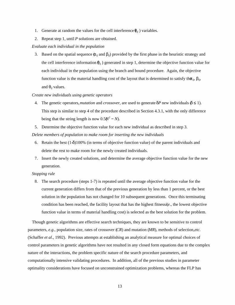
1. Generate at random the values for the cell interference (θij ) variables.

2. Repeat step 1, until P solutions are obtained.

Evaluate each individual in the population

3. Based on the spatial sequence (α ij and βij) provided by the first phase in the heuristic strategy and

the cell interference information (θij ) generated in step 1, determine the objective function value for

each individual in the population using the branch and bound procedure. Again, the objective

function value is the material handling cost of the layout that is determined to satisfy the α ij, βij,

and θij values.

Create new individuals using genetic operators

4. The genetic operators, mutation and crossover, are used to generate δP new individuals (δ ≤ 1).

This step is similar to step 4 of the procedure described in Section 4.3.1, with the only difference

being that the string length is now 0.5(N2 − N).

5. Determine the objective function value for each new individual as described in step 3.

Delete members of population to make room for inserting the new individuals

6. Retain the best (1-δ)100% (in terms of objective function value) of the parent individuals and

delete the rest to make room for the newly created individuals.

7. Insert the newly created solutions, and determine the average objective function value for the new

generation.

Stopping rule

8. The search procedure (steps 1-7) is repeated until the average objective function value for the

current generation differs from that of the previous generation by less than 1 percent, or the best

solution in the population has not changed for 10 subsequent generations. Once this terminating

condition has been reached, the facility layout that has the highest fitness (i.e., the lowest objective

function value in terms of material handling cost) is selected as the best solution for the problem.

Though genetic algorithms are effective search techniques, they are known to be sensitive to control

parameters, e.g., population size, rates of crossover (CR) and mutation (MR), methods of selection, etc.

(Schaffer et al., 1992). Previous attempts at establishing an analytical measure for optimal choices of

control parameters in genetic algorithms have not resulted in any closed form equations due to the complex

nature of the interactions, the problem specific nature of the search procedure parameters, and

computationally intensive validating procedures. In addition, all of the previous studies in parameter

optimality considerations have focused on unconstrained optimization problems, whereas the FLP has

14

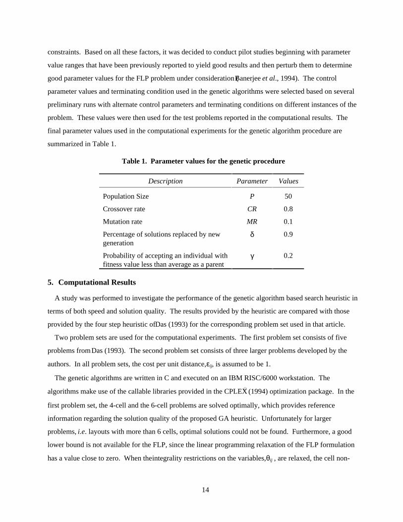
constraints. Based on all these factors, it was decided to conduct pilot studies beginning with parameter

value ranges that have been previously reported to yield good results and then perturb them to determine

good parameter values for the FLP problem under consideration (Banerjee et al., 1994). The control

parameter values and terminating condition used in the genetic algorithms were selected based on several

preliminary runs with alternate control parameters and terminating conditions on different instances of the

problem. These values were then used for the test problems reported in the computational results. The

final parameter values used in the computational experiments for the genetic algorithm procedure are

summarized in Table 1.

Table 1. Parameter values for the genetic procedure

Description Parameter Values

Population Size P 50

Crossover rate CR 0.8

Mutation rate MR 0.1

Percentage of solutions replaced by newgeneration

δ 0.9

Probability of accepting an individual withfitness value less than average as a parent

γ 0.2

5. Computational Results

A study was performed to investigate the performance of the genetic algorithm based search heuristic in

terms of both speed and solution quality. The results provided by the heuristic are compared with those

provided by the four step heuristic of Das (1993) for the corresponding problem set used in that article.

Two problem sets are used for the computational experiments. The first problem set consists of five

problems from Das (1993). The second problem set consists of three larger problems developed by the

authors. In all problem sets, the cost per unit distance, εij, is assumed to be 1.

The genetic algorithms are written in C and executed on an IBM RISC/6000 workstation. The

algorithms make use of the callable libraries provided in the CPLEX (1994) optimization package. In the

first problem set, the 4-cell and the 6-cell problems are solved optimally, which provides reference

information regarding the solution quality of the proposed GA heuristic. Unfortunately for larger

problems, i.e. layouts with more than 6 cells, optimal solutions could not be found. Furthermore, a good

lower bound is not available for the FLP, since the linear programming relaxation of the FLP formulation

has a value close to zero. When the integrality restrictions on the variables, θij , are relaxed, the cell non-

15

overlap constraints are no longer enforced. Therefore, all cells are placed on top of each other, which

results in a small objective function value.

Das (1993) reports results for the four-step heuristic solving the problems in set 1. These results are

repeated in column 4 of Table 1, labeled “original four-step.” Since the computation times for the four-

step heuristic were not reported in the paper, the authors implemented the four-step heuristic from Das

(1993) to obtain some estimate of the computation times. Because these times turned out to be very long, a

computational time limit of 72000 seconds was set for the second step, which has the longest computation

time in the four-step heuristic. When this time limit was reached, the best known integer feasible solution

was recorded and passed to the third step. The columns labeled “four-step” refer to our implementation of

the four-step heuristic. It must be noted that Das’s original results are better in some cases, suggesting that

very long run times were allowed or some specialized procedures were used to solve the four-step

subproblems. The complete experimental results are summarized in Table 1, Table 2, and Figure 4.

Table 1. Material flow costs for problem set 1

No.cells

Optimal OriginalFour-step

Four-step GAProcedure

GAimprovement

4 1393.6 1679.4 1631.6 1393.6* 17.08%

6 2612.7 2620.0 3163.4 2612.7* 21.08%

8 N/A 10777.1 10374.1 9174.8 13.07%

10 N/A 15878.3 20791.4 19777.3 5.13%

12 N/A 41267.5 49082.5 45353.5 8.22%

* Optimal solution obtained using the GA procedure

Table 2. Material flow costs for problem set 2

No. ofcells

GAProcedure

14 51154.5

16 64371.4

18 78567.8

16

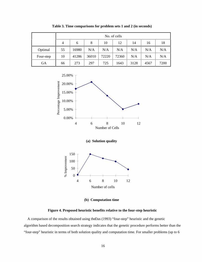
Table 3. Time comparisons for problem sets 1 and 2 (in seconds)

No. of cells

4 6 8 10 12 14 16 18

Optimal 55 16980 N/A N/A N/A N/A N/A N/A

Four-step 10 41286 36010 72220 72360 N/A N/A N/A

GA 66 273 297 725 1643 3128 4567 7200

0.00%

5.00%

10.00%

15.00%

20.00%

25.00%

4 6 8 10 12Number of Cells

Pe

rce

nta

ge I

mpr

ove

me

nt

(a) Solution quality

0

50

100

150

4 6 8 10 12

Number of cells

% I

mpr

ove

me

nt

(b) Computation time

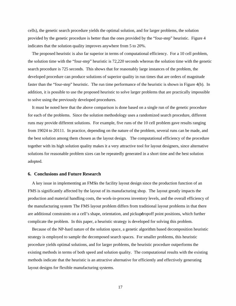
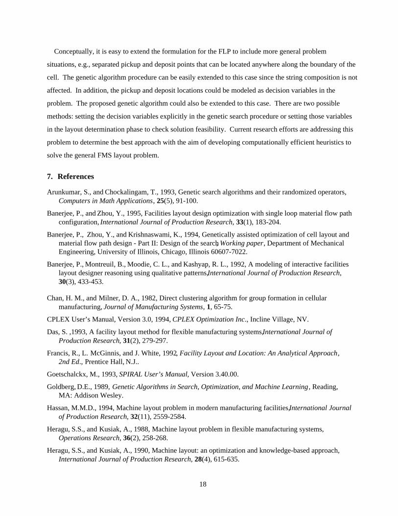
Figure 4. Proposed heuristic benefits relative to the four-step heuristic

A comparison of the results obtained using the Das (1993) “four-step” heuristic and the genetic

algorithm based decomposition search strategy indicates that the genetic procedure performs better than the

“four-step” heuristic in terms of both solution quality and computation time. For smaller problems (up to 6

17

cells), the genetic search procedure yields the optimal solution, and for larger problems, the solution

provided by the genetic procedure is better than the ones provided by the “four-step” heuristic. Figure 4

indicates that the solution quality improves anywhere from 5 to 20%.

The proposed heuristic is also far superior in terms of computational efficiency. For a 10 cell problem,

the solution time with the “four-step” heuristic is 72,220 seconds whereas the solution time with the genetic

search procedure is 725 seconds. This shows that for reasonably large instances of the problem, the

developed procedure can produce solutions of superior quality in run times that are orders of magnitude

faster than the “four-step” heuristic. The run time performance of the heuristic is shown in Figure 4(b). In

addition, it is possible to use the proposed heuristic to solve larger problems that are practically impossible

to solve using the previously developed procedures.

It must be noted here that the above comparison is done based on a single run of the genetic procedure

for each of the problems. Since the solution methodology uses a randomized search procedure, different

runs may provide different solutions. For example, five runs of the 10 cell problem gave results ranging

from 19024 to 20111. In practice, depending on the nature of the problem, several runs can be made, and

the best solution among them chosen as the layout design. The computational efficiency of the procedure

together with its high solution quality makes it a very attractive tool for layout designers, since alternative

solutions for reasonable problem sizes can be repeatedly generated in a short time and the best solution

adopted.

6. Conclusions and Future Research

A key issue in implementing an FMS is the facility layout design since the production function of an

FMS is significantly affected by the layout of its manufacturing shop. The layout greatly impacts the

production and material handling costs, the work-in-process inventory levels, and the overall efficiency of

the manufacturing system The FMS layout problem differs from traditional layout problems in that there

are additional constraints on a cell’s shape, orientation, and pickup/dropoff point positions, which further

complicate the problem. In this paper, a heuristic strategy is developed for solving this problem.

Because of the NP-hard nature of the solution space, a genetic algorithm based decomposition heuristic

strategy is employed to sample the decomposed search spaces. For smaller problems, this heuristic

procedure yields optimal solutions, and for larger problems, the heuristic procedure outperforms the

existing methods in terms of both speed and solution quality. The computational results with the existing

methods indicate that the heuristic is an attractive alternative for efficiently and effectively generating

layout designs for flexible manufacturing systems.

18

Conceptually, it is easy to extend the formulation for the FLP to include more general problem

situations, e.g., separated pickup and deposit points that can be located anywhere along the boundary of the

cell. The genetic algorithm procedure can be easily extended to this case since the string composition is not

affected. In addition, the pickup and deposit locations could be modeled as decision variables in the

problem. The proposed genetic algorithm could also be extended to this case. There are two possible

methods: setting the decision variables explicitly in the genetic search procedure or setting those variables

in the layout determination phase to check solution feasibility. Current research efforts are addressing this

problem to determine the best approach with the aim of developing computationally efficient heuristics to

solve the general FMS layout problem.

7. References

Arunkumar, S., and Chockalingam, T., 1993, Genetic search algorithms and their randomized operators,Computers in Math Applications, 25(5), 91-100.

Banerjee, P., and Zhou, Y., 1995, Facilities layout design optimization with single loop material flow pathconfiguration, International Journal of Production Research, 33(1), 183-204.

Banerjee, P., Zhou, Y., and Krishnaswami, K., 1994, Genetically assisted optimization of cell layout andmaterial flow path design - Part II: Design of the search, Working paper, Department of MechanicalEngineering, University of Illinois, Chicago, Illinois 60607-7022.

Banerjee, P., Montreuil, B., Moodie, C. L., and Kashyap, R. L., 1992, A modeling of interactive facilitieslayout designer reasoning using qualitative patterns, International Journal of Production Research,30(3), 433-453.

Chan, H. M., and Milner, D. A., 1982, Direct clustering algorithm for group formation in cellularmanufacturing, Journal of Manufacturing Systems, 1, 65-75.

CPLEX User’s Manual, Version 3.0, 1994, CPLEX Optimization Inc., Incline Village, NV.

Das, S. ,1993, A facility layout method for flexible manufacturing systems, International Journal ofProduction Research, 31(2), 279-297.

Francis, R., L. McGinnis, and J. White, 1992, Facility Layout and Location: An Analytical Approach,2nd Ed., Prentice Hall, N.J..

Goetschalckx, M., 1993, SPIRAL User’s Manual, Version 3.40.00.

Goldberg, D.E., 1989, Genetic Algorithms in Search, Optimization, and Machine Learning, Reading,MA: Addison Wesley.

Hassan, M.M.D., 1994, Machine layout problem in modern manufacturing facilities, International Journalof Production Research, 32(11), 2559-2584.

Heragu, S.S., and Kusiak, A., 1988, Machine layout problem in flexible manufacturing systems,Operations Research, 36(2), 258-268.

Heragu, S.S., and Kusiak, A., 1990, Machine layout: an optimization and knowledge-based approach,International Journal of Production Research, 28(4), 615-635.

19

Holland, J.H., 1992, Genetic algorithms, Scientific American, July, 66-72.

Jacob, F.R., 1987, A layout planning system with multiple criteria and a variable domain representation,Management Science, 33, 1020-1034.

Kusiak, A. and Heragu, S.S., 1987, The facility layout problem, European Journal of OperationalResearch, 29, 229-251.

Lee, H., and Garcia-Diaz, A., 1993, A network flow approach to solve clustering problems in grouptechnology, International Journal of Production Research, 31(3), 603-612.

Luggen, W.W., 1991, Flexible Manufacturing Cells and Systems, Englewood Cliffs, Prentice-Hall, NJ.

Meller, R.D., and Gau, K-Y., 1996, The facility layout problem: recent and emerging trends andperspectives, Journal of Manufacturing Systems, 15(5), 351-366.

Schaffer, J.D., Whitley, D., and Eshelman, L.J., 1992, Combinations of genetic algorithms and neuralnetworks: a survey of the state of the art, Proceedings of the International Conference on theCombinations of Genetic Algorithms, San Mateo, CA: Morgan Kaufmann Publishers.

Syswerda, G., 1989, Uniform crossover in genetic algorithms, Proceedings of the Third InternationalConference on Genetic Algorithms, San Mateo, Calif.: Morgan Kaufmann Publishers.

Tompkins, J.A., and White, J.A., 1984, Facilities Planning, Wiley and Sons, New York, NY.

Whitley, D., 1988, GENITOR: A different genetic algorithm, Proceedings of the Rocky MountainConference on Artificial Intelligence, Denver.

a genetic algorithm for facility layout design in flexible ... · pdf filea genetic algorithm...

Documents