A Generative Kriging Surrogate Model for Constrainedand Unconstrained Multi-objective Optimization∗

Rayan Hussein and Kalyanmoy DebComputational Optimization and Innovation (COIN) Laboratory

Department of Electrical and Computer EngineeringMichigan State University

East Lansing, MI 48824, USA{husseinr,kdeb}@egr.msu.edu, http://www.egr.msu.edu/˜kdeb/

COIN Report Number 2016007

March 28, 2016

Abstract

Surrogate models are effective in reducing the computational time required for solvingoptimization problems. However, there have been a lukewarm interest in finding multipletrade-off solutions for multi-objective optimization problems using surrogate models. Theliterature on surrogate modeling for constrained optimization problems is also rare. The dif-ficulty lies in the requirement of building and solving multiple surrogate models, one for eachPareto-optimal solution. In this paper, we first provide a brief introduction of the past stud-ies and suggest a computationally fast, Kriging-based, and generative procedure for findingmultiple near Pareto-optimal solutions in a systematic manner. The expected improvementmetric is maximized using a real-parameter genetic algorithm for finding new solutions forhigh-fidelity evaluations. The approach is computationally fast due to the interlinking ofbuilding multiple surrogate models and in its systematic sequencing methodology for assist-ing one model with another. In standard two and three-objective test problems with andwithout constraints, our proposed methodology takes only a few hundreds of high-fidelitysolution evaluations to find a widely distributed near Pareto-optimal solutions compared tothe standard EMO methods requiring tens of thousands of high-fidelity solution evaluations.The framework is generic and can be extended to utilize other surrogate modeling methodseasily.

∗Accepted in GECCO-2016 Conference (20-24 July, 2016), Denver, Colorado, USA.

1

1 Introduction

In most practical optimization problems, the evaluation of a solution involves computation-ally expensive softwares and procedures, which remain as one of the main bottlenecks ofcompleting an optimization run within a reasonable amount of time. However, it is clearthat since solutions created in the beginning of an optimization simulation are expected tobe away from the optimal region and an exact and precise evaluation of the solution may notbe necessary. As the solutions progress towards the optimal region, a more precise evaluationmay be invoked.

The recent developments of optimization methods have led to an increasing interestof approximation models or surrogate models [1, 2, 3]. A surrogate model approximatesthe original objective or constraint function by computing a few high-fidelity solutions –solutions that are evaluated using the original but computationally expensive functions. Mostsurrogate models are designed in a way so as to pass through these high-fidelity solutions,such as Kriging models [4], but there exist some methods that makes a regression fit of thehigh-fidelity solutions. The optimization process is then continued using the surrogate modeluntil the model is deemed to be accurate enough in the current region of focus. Due to thisreason, surrogate models are effective in reducing the overall computational time required inreal-world design optimization.

Despite the existence of a plethora of surrogate modeling study in the context of single-objective optimization problems, there is not much efforts spent on extending the ideas tomulti-objective optimization. The reasons for the lack of study, except a few [5, 2] is that inmulti-objective optimization, the aim is to find multiple trade-off Pareto-optimal solutions,instead of a single optimal solution. Most surrogate modeling studies have not consideredmodeling a multi-modal function in the spirit of locating multiple optimal solutions simul-taneously. Hence, there is not much clue that can be borrowed from the single-objectiveliterature. However, Emmerich et al [5] have generalized the probability of improvement andthe expected improvement concept to multi-objective optimization. Single-objective EAs areused for maximizing one of these metrics for determining which point should be evaluatednext. Although one can select multiple test points with high-metric values at each iteration,these scalar metrics on their own could not predict the most likely shape and location ofthe whole PF. Therefore, they may not be stochastically sound for locating multiple testpoints. Another study [2] used a generative method of approximating the objective functionfor a single Pareto-optimal solution at a time. However, the study did not consider anyconstraint, which is a major issue in making surrogate modeling methods practical. It isironical that while surrogate models are used to make optimization methods practical, buton the other hand the methods are flexible enough to handle other important practicalities,such as constraint and uncertainty handling. This work is motivated by the later study,but enables the use of constraints and other efficient features that make the overall algo-rithm computationally fast and applicable to larger-sized problems than the above existingmethodologies have demonstrated.

In the remainder of this paper, we provide a brief summary of the efficient global op-timization (EGO) procedure and some past surrogate modeling studies in the context ofmulti-objective optimization in Section 2. The proposed multi-objective EGO procedure isthen described in detail in Section 3. Results on unconstrained and constrained test prob-

2

lems are then presented in Section 4. Finally, conclusions and extensions of this study arediscussed in Section 5.

2 Efficient Global Optimization

(EGO)

One of the popular surrogate models used in approximating computationally expensive func-tions is the well-known Kriging model. Kriging methodology was proposed by Daniel G.Krige [6] to predict the spatial patterns for gold mines. Then, more improvements to theKriging Model we developed by Matheron [7]. On other hand, Sacks et al [8] utilized the Krig-ing model to improve the approximation of computer experiments. Later, Kriging method-ology was also called the design and analysis of computer experiments (or DACE) stochasticprocess model [9].

The DACE is one of the efficient tools for dealing with expensive single-objective op-timization problems. In this methodology, the approximation of a function in terms of adesign variable is considered as a sample of Gaussian stochastic process. Then, the distri-bution of the function value at any untested point can be estimated using Kriging model.Jones et al [10] proposed a practical approach to determine the location of additional samplepoints which improves the Kriging model accuracy. This is known as the Efficient GlobalOptimization (EGO) procedure. On the Kriging model, EGO searches for the location wherethe expected improvement of the original function is maximized, and then reconstructs thesurrogate model by adding a new sample point at this location. This approach consists ofthe following steps:

Step 1: Build an initial Kriging model for the objective function.

Step 2: Use a cross-validation method to ensure that the Kriging prediction and measureof uncertainty are satisfactory.

Step 3: Find the location that maximizes the expected improvement (EI) function.

Step 4: Evaluate the point at which the EI function was maximum. Update the Krigingmodel using the new point and move to Step 3.

There exists a large number of studies to incorporate Kriging model into evolutionaryalgorithm (EA) for only single-objective optimization problems [11]. Therefore, our proposedmethod is dealing with Multi-objective optimization problems based on Kriging model. Abrief overview of Kriging methodology is presented in the following sections.

2.1 Overview of Kriging Method

The Kriging approach treats the function of interest as a realization of a random function(stochastic process) y(x) . For this reason, the mathematical model of Kriging method hasbeen presented as a linear combination of a global model plus its departure:

y(x) = f(x) + Z(x), (1)

3

where y(x) is the unknown deterministic response, f(x) is a known function of x, and Z(x)is a realization of a stochastic process with zero mean, σ2 variance, and having non-zerocovariance values. The procedure starts with obtaining a sample data of limited size (i.e. n-

design sets each having k-variables), X ={x(1), x(2), . . . , x(n)

}T, and a corresponding vector

of scalar responses, Y ={y(1), y(2), . . . , y(n)

}T. It is assumed that if any two design points,

e.g. x(i) and x(j), are positioned close together in the design space, their respective functionvalues y(i) and y(j) are also expected to be similar. Usually, the Latin hypercube techniqueis used to create initial point, ensuring a diverse set of points along each variable dimension[1].

2.2 Kriging Procedure

Without going to the detailed mathematics, here, we provide the Kriging predictor, as fol-lows:

y(x) = µ+ r(x∗, x)TR−1(y(x)− 1µ), (2)

where r(x∗, x) is the linear vector of correlation between the unknown point x to be predictedand the known sample points x∗. R denote the n × n matrix with (i, j) whose entry isCorr[y(i), y(j)], and 1 denote an n-vector of ones. The optimal values of µ and σ2, expressedas function of R are given below[10]:

µ =1TR−1y

1TR−11, (3)

σ2 =(~y − 1µ)TR−1(~y − 1µ)

n. (4)

Moreover, Kriging is attractive because of its ability to provide error estimates of the pre-dictor:

s2(x) = σ2[1− rTR−1r +(1− rTR−1r)2

1TR−11]. (5)

2.3 The Expected Improvement Procedure

As described in the previous section, using Kriging technique in optimization requires fittingthe Kriging model, finding the point that maximizes expected improvement, evaluating thefunction at this point, and ultimately iterating. The second step of this procedure is basedon the fact that Kriging helps in estimating the model uncertainty and stresses on exploringpoints where we are uncertain. In order to do this, Kriging method treats the value of thefunction at x as if it were the realization of a stochastic process y(x), with the mean givingby the predictor y(x) and variance s(x), The expected improvement function is given asfollows [10, 4]:

E[I(x)]) = (ybest − y(x))Φ

(ybest − y(x)

s(x)

)+ s(x)φ

(ybest − y(x)

s(x)

), (6)

where Φ(.) and φ(.) are the normal cumulative distribution function and probability densityfunction, respectively. It is worth noting here that the implementation of Kriging (DACE)is based on universal Kriging, where it is possible to use other regression models as well.

4

The decision of to select Kriging method as an approximator depends on various factors.One important factor is the size of the search space. It has been observed that Krigingmethodology does not work very well when the number of variables exceeds about 10.

As mentioned above, Kriging and subsequent EGO methodology are standards in thecontext of single-objective unconstrained problems, but they have not been extended wellneither to constrained single-objective problems nor to multi-objective optimization prob-lems. A recent study [12] suggested a way to modify the expected improvement function forconstrained problems. It selects the best feasible objective function value instead of ybest inEquation 6. This method has been applied only to single objective optimization problems.The expected improvement function is modified as follows:

Ec[I(x)] = E[I(x)]ΠJj=1Fj(x), (7)

where Fj(x) is given as follows for j-th constraint:

Fj(x) =

0.5 + 0.5erf

(gj(x)

sj(x)

), if erf

(gj(x)

sj(x)

)≥ 1,

2− erf(

gj(x)

sj(x)

), if 0 < erf

(gj(x)

sj(x)

)< 1,

0, otherwise,

(8)

where gj(x) is the normalized version of j-th constraint function, and sj is the MSE predictionof the j-th constraint function. It is clear that if any constraint is violated, Ec[I(x)] is zeroand for near constraint boundary solutions Ec[I(x)] has a large value, thereby emphasizingnear-boundary solutions during simulations, and for points that are well inside the feasibleregion Ec[I(x)] = E[I(x)]. Here, we do not use this method, instead, handle constraintdirectly through a modeling of the selection function, as discussed in Section 3.

In the following subsection, we provide a few existing studies of Kriging method formulti-objective optimization problems.

2.4 Past Studies on Surrogate-based EMO

ParEGO, proposed by Knowles [13], applies the EGO algorithm and the selected aggregationfunction randomly for finding a point to evaluate the next point in the search space. Themajor drawback of the ParEGO algorithm is that it considers one aggregation function ateach iteration and it is not able to generate multiple candidate points at one iteration. S-Metric Selection based EGO (SMS-EGO) [14] extends the idea of Emmerich et al. [5] andoptimizes the S-metric, a hypervolume-based metric, by the covariance matrix adaptationevolution strategy (CMS-ES) algorithm to decide which point will be evaluated next. LikeParEGO, SMS-EGO evaluates only one single test point at each iteration.

MOEA/D-EGO, proposed by Zhang et al. [2], integrates the EGO algorithm with de-composition based multi-objective EAs (MOEA/D) [15]. MOEA/D is based on conventionalaggregation approach. It decomposes an MOP into a number of single-objective optimiza-tion subproblems. At each iteration in MOEA/D-EGO, a Gaussian stochastic process modelfor each subproblem is built based on data obtained from the previous search, and the ex-pected improvement of these subproblems are optimized simultaneously by using MOEA/Dprocedure for generating a set of candidate solutions. Then, a few of them are selected for

5

evaluation. This algorithm was applied to unconstrained multi-objective ZDT problems [16]having only eight variables, although the original test problems were defined for 30 variables.It is likely that Kriging method could not approximate a 30-dimensional problem well andthe overall method suffered from the curse of dimensionality. Moreover, the method did notuse any constraint in the study; hence an extension to multi-objective constrained problemsis not clear.

3 Proposed Multi-objective EGO Method

With the brief description of the EGO method for single-objective optimization problemsdiscussed above, we are now ready to provide details of our proposed procedure.

Our proposed approach is a generative multi-objective optimization procedure in whichone Pareto-optimal point is determined to be found at a time. The development of a suitablesurrogate modeling and its solution are achieved for one targeted Pareto-optimal solution ata time. However, the surrogate building process for multiple Pareto-optimal solutions arenot all independent to each other, rather the whole process is interlinked, as described bythe following step-by-step procedure.

Step 1: Create an archive having H random points based on Latin hypercube sampling(LHS) [1] from the entire variable search space. Evaluate each of these solutions usingthe objective and constraint functions (referred to as ‘high-fidelity’ evaluations).

Step 2: Generate R reference directions on a normalized unit hyperplane in the objectivespace using Das and Dennis’s method [17]. Then, for each reference direction chosenusing a Diversity Preserver procedure, execute the following steps.

Step 3: Select K points closest to the reference direction based on projected Euclideandistance of all H archive points in the objective space using a Points Selector pro-cedure.

Step 4: Build a local surrogate model (Surrogate Model procedure) using the chosen αHpoints executed already with high-fidelity evaluations (for example α = 0.7).

Step 5: Use the developed surrogate model to find the best possible solution of the modelby a specific (Optimization) procedure.

Step 6: Perform a high-fidelity evaluation of the newly created solution and add it to thearchive.

Step 7: Repeat Steps 3 to 6 p times to add p new solutions to the archive.

Step 8: Move to a new reference line according to the Diversity Preserver procedure andGo to Step 3 until all reference lines are considered or another termination criterion issatisfied.

The above step-by-step procedure is a generic surrogate-based EMO procedure that canbe applied with any surrogate modeling technique and optimization algorithm. It also hasa few other flexibilities which we describe next.

6

3.1 Diversity Preserver Procedure

This procedure provides the linking between model building and its solution among severalreference lines. Given K reference directions spanning the entire first quadrant of the M -dimensional objective space, this procedure determines the sequence of choosing referencelines. Figure 1 illustrates the proposed procedure in which H = 20 random points denotethe archive and for each of five reference directions, K = 4 points are chosen.

Figure 1: An illustration of the proposed surrogate-based generative EMO procedure

This procedure involves fixing the following three entities:

1. The starting reference direction,

2. The sequence of choosing reference directions, and

3. Repeat pattern of the sequencing.

The surrogate modeling can start anywhere, but either one of the extreme reference directions(lying on one of the objective directions) or in the middle of the objective space (equi-distancefrom all objective directions) are two unbiased approaches. In all our study here, we considerthe former approach of choosing one of the objective axis direction as the initial referencedirection.

The second entity is probably the most important factor. Once the initial direction ischosen, a model is built and one or more solutions are obtained using the model, whichreference direction to choose next is a relevant question.

In the neighborhood approach, we can choose one of the nearest reference direction tothe already chosen directions as the next direction. Since there is one or more models al-ready built around a neighboring reference direction in this approach, inclusion of their bestsolutions in the neighboring model building process should create a better model. How-ever, the flip side is that each model then have a local perspective and the performance ofthis approach will depend on the mapping between variable and objective spaces. In the

7

maximum diversity approach, a reference direction which is maximally away from all cho-sen reference directions is selected for building the next surrogate model. In this approach,initial few models are independent to each other, but together they will span the searchspace well. Later surrogate models tend to have a more global perspective than those in theneighborhood approach. We use both approaches in this study.

Another aspect of the diversity preserving procedure is whether the above sequencingprocess needs to be repeated after their first pass on all reference directions! This can bedecided adaptively, based on whether a satisfactory set of non-dominated solutions havebeen found for each reference direction. If it is to repeated, an exactly the same sequencingor a different sequencing operation can be chosen as well. The repetition need not for allreference directions, the ones that generated a dominated solution can be repeated. Forrepetition, it will be a good idea to preserve all surrogate models generated in the first passof the procedure. In this study, we repeat the first pass in the same sequence one more time.

3.2 Points Selector Procedure

In this procedure, a set of K points will be chosen from the archive having H points. Here,we suggest to compute the orthogonal distance of each archive point to the given referencedirection and select K shortest orthogonal distance solutions. But other distance metrics(such as the achievement scalarization function (ASF) value or its augmented version) orTchebyshev metric or other Lp norms can be used, instead.

3.2.1 Achievement Scalarization Function (ASF)

One of the common ways to solve the generic multi-objective optimization problem is to solvea parameterized achievement scalarization function (ASF) optimization problem repeatedlyfor different parameter values. The ASF approach was originally suggested by Wierzbicki[18].For a specified reference point z and a weight vector w (parameters of the ASF problem),the ASF problem is given as follows:

Minimizex ASF(x, z, w) = maxMi=1

(fi(X)−zi

wi

),

Subject to gj(X) ≤ 0, j = 1, 2, . . . , J.(9)

The reference point z ∈ RM is any point in the M -dimensional objective space and theweight vector w ∈ RM is an M -dimensional unit vector for which every wi ≥ 0 and |W | = 1.To avoid division by zero, we shall consider strictly positive weight values. It has beenproven that for above conditions of z and w, the solution to the above problem is always aPareto-optimal solution [19]. Figure 2 illustrates the ASF procedure of arriving at a weakor a strict Pareto-optimal solution.

For illustrating the working principle of the ASF procedure, we consider specific referencevector z (marked in the figure) and weight vector w (marked as w in the figure). For any pointx, the objective vector f is computed (shown as F). Larger of two quantities (f1 − z1)/w1

and (f2− z2)/w2) is then chosen as the ASF value of the point x. For the point G, the abovetwo quantities are identical, that is, (f1 − z1)/w1 = (f2 − z2)/w2 = p (say). For points online GH, the first term dominates and the ASF value is identical to p. For points on line

8

w

z

B

Obj1

A Iso−ASFline for B

(f1−z1)D

=(z1,z2)

=(w1,w2)

G

F=(f1,f2)

(f2−

z2)

K

H1/w1

1/w2

O

Obj2

Figure 2: ASF procedure of finding a Pareto-optimal solution is illustrated.

GK, the second term dominates and the ASF value is also identical to p. Thus, it is clearthat for any point on lines GH and GK, the corresponding ASF value will be the same asp. This is why an iso-ASF line for an objective vector at F traces any point on lines KGand GH. For another point A, the iso-ASF line is shown in dashed lines passing throughA, but it is important to note that its ASF value will be larger than p, since its iso-ASFlines meet at the w-line away from the direction of minimum of both objectives. Since theASF function is minimized, point F is considered better than A in terms of the ASF value.Similarly, point A will be considered better than point B. A little thought will reveal thatwhen the ASF problem is optimized the point O will correspond to the minimum ASF valuein the entire objective space (marked with a shaded region), thereby making point O (anefficient point) as the final outcome of the optimization problem stated in Equation 9 for thechosen z and w vectors. By keeping the reference point z fixed and by changing the weightvector w (treating it like a parameter of the resulting scalarization process), different pointson the efficient front can be generated by the above ASF minimization process.

The ASF procedure calculated from an ideal or an utopian point may result in a weakPareto-optimal solution [20]. To avoid finding weak points, the following augmented ASFcomputation is used [19]:

Minimizex AASF(x, z, w) = maxMi=1

(fi(X)−zi

wi

)+ρ∑M

j=1

(fi(X)−zi

wi

),

Subject to gj(X) ≤ 0, j = 1, 2, . . . , J.

(10)

Here, the parameter ρ takes a small value (∼ 10−3). The additional term on the objectivefunction has an effect of making the iso-AASF lines inclined to objective axes.

9

3.3 Surrogate Model Procedure

This is one of the main procedures that will affect the performance of the overall algorithm.Here, we use the Kriging methodology [4] to model the selection function used for comparingsolutions in the presence/absence of constraints. The selection function is given below:

S(x) =

{f(x), if x is feasible,fmax + CV(x), otherwise.

(11)

It is assumed that the objective function is minimized and there are J constraints of typegj(x) ≤ 0 (j = 1, 2, . . . , J). Equality constraints are converted into two inequality constraintsof the above type. Here, the parameter fmax is the worst objective function value of allfeasible solutions of K solutions used for building the model. The function CV(x) is theoverall constraint violation, defined as follows:

CV(x) =J∑

j=1

〈gj(x)〉, (12)

where the bracket operator 〈α〉 is −α if α < 0 and zero, otherwise. The function gj is anormalized version of constraint function gj [21].

Thus, for a given set of K points to build the Kriging model, the above unconstrainedselection function S(x) for each point x is computed and the standard Kriging modelingtechnique [4] is used to find the estimator and the mean squared error (MSE) function.Thereafter, the expected improvement function [10] is formulated for the next step.

Here, other surrogate modeling methods can also be used, instead of the Kriging method-ology. We are currently working with a few other surrogate models for this purpose.

3.4 Optimization Procedure

Once the surrogate model is built, the next step is to optimize the model to find the bestpossible solution of the model. For this purpose, we use a real-parameter genetic algorithm(rGA) which uses simulated binary crossover [22] and polynomial mutation operator [20].The population is started with a random population and rGA is run for 100 number ofgenerations. Here, the rGA population can be initialized by the K points used to build thesurrogate model.

Figure 1 illustrates the overall procedure. It can be observed that some of the originalarchive points may not have been chosen for any of the reference directions, particularly whenK is very small compared to H. Also, some points can be chosen for more than one referencedirections, particularly when K is comparable to H. Since all H points were already madehigh-fidelity evaluations, it is better to choose K in a way so that all H evaluated solutionsare used for one or more reference directions. Another advantage of the proposed methodis that since the points chosen for a surrogate model for a particular reference direction areclose to each other, each model will be local to the reference direction and is likely find therespective Pareto-optimal solution more reliably than if the model was a global spanning theentire search space. Since each surrogate model uses a few points to build it, the proposedalgorithm is also likely to be computationally faster than global models.

10

4 Results

In this section, we compare our proposed multi-objective EGO method with MOEA/D-EGO procedure, proposed elsewhere [2]. We mentioned in the previous section, MOEA/D-EGO solved ZDT problems with only eight variables and solved only one test problem(DTLZ2) having three objective functions. Our multi-objective EGO is applied to 30-variableversion of the ZDT problems, also to the constrained test problems, and multiple three-objective test problems. The reference direction that used in most of instances test problemsis neighborhood approach as we illustrated in Section 3.

The rGA control parameters are set as follows:

• Population size = 10k, where k is a number of variables.

• Number of generations = 100.

• Crossover probability = 0.9.

• Mutation probability = 1/k.

• Distribution index for SBX operator = 2.

• Distribution index for polynomial mutation operator = 20.

4.1 Two-Objective Unconstrained Problems

First, we compare our multi-objective EGO with MOEA/D-EGO on ZDT1 and ZDT2 prob-lems for an identical number of variables (k = 8). As reported in the original study [2],MOEA/D-EGO requires 200 high-fidelity function evaluations for ZDT1 and ZDT2, whileour method takes 164 function evaluations for ZDT1 and 122 function evaluations for ZDT2,respectively, to have almost a similar number of non-dominated solutions, as illustrated inFigures 3 and 4 respectively.

Next, we apply our multi-objective EGO method to solve ZDT1, ZDT2, and ZDT3 with30 variables (the original size). In our knowledge, this is the first time a meta-modelingmethod has attempted to solve the original version of ZDT test problems. ZDT1 takes 858function evaluations with 51 reference directions, ZDT2 takes 276 function evaluations with21 reference directions, and ZDT3 takes 1,170 function evaluations with 51 reference direc-tions. The Pareto-optimal front of these problems and obtained non-dominated solutionsare shown in Figures 5 and 6 (a), respectively. For ZDT6 problem having 10 variables, ourmethod takes 558 function evaluations with 51 reference directions, as illustrated in Figure 6(b).

ZDT4 problem is multi-modal for any Kriging methodology. The previous study [2] didnot show results and our approach was also not able to find solutions close to the truePareto-optimal front.

4.2 Three-Objective Problems

Regarding the three-objective optimization problems, the MOEA/D-EGO solved the sim-plest problem (DTLZ2) with only six variables which takes 300 solution evaluations. Our

11

Figure 3: ZDT1 with eight decision variable (a) MOEA/D-EGO, (b) Multi-objective EGO

Figure 4: ZDT2 with eight decision variable (a) MOEA/D-EGO, (b) Multi-objective EGO

12

Figure 5: (a) Multi-objective EGO for thirty-variable ZDT1, (b) Multi-objective EGO forthirty-variable ZDT2

Figure 6: (a) Multi-objective EGO for thirty-variable ZDT3, (b) Multi-objective EGO forten-variable ZDT6

13

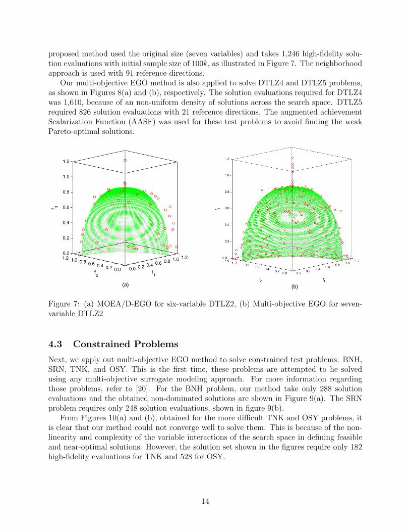
proposed method used the original size (seven variables) and takes 1,246 high-fidelity solu-tion evaluations with initial sample size of 100k, as illustrated in Figure 7. The neighborhoodapproach is used with 91 reference directions.

Our multi-objective EGO method is also applied to solve DTLZ4 and DTLZ5 problems,as shown in Figures 8(a) and (b), respectively. The solution evaluations required for DTLZ4was 1,610, because of an non-uniform density of solutions across the search space. DTLZ5required 826 solution evaluations with 21 reference directions. The augmented achievementScalarization Function (AASF) was used for these test problems to avoid finding the weakPareto-optimal solutions.

(a) (b)

Figure 7: (a) MOEA/D-EGO for six-variable DTLZ2, (b) Multi-objective EGO for seven-variable DTLZ2

4.3 Constrained Problems

Next, we apply out multi-objective EGO method to solve constrained test problems: BNH,SRN, TNK, and OSY. This is the first time, these problems are attempted to he solvedusing any multi-objective surrogate modeling approach. For more information regardingthose problems, refer to [20]. For the BNH problem, our method take only 288 solutionevaluations and the obtained non-dominated solutions are shown in Figure 9(a). The SRNproblem requires only 248 solution evaluations, shown in figure 9(b).

From Figures 10(a) and (b), obtained for the more difficult TNK and OSY problems, itis clear that our method could not converge well to solve them. This is because of the non-linearity and complexity of the variable interactions of the search space in defining feasibleand near-optimal solutions. However, the solution set shown in the figures require only 182high-fidelity evaluations for TNK and 528 for OSY.

14

Figure 8: (a) Multi-objective EGO for seven-variable DTLZ4, (b) Multi-objective EGO forseven-variable DTLZ5

Figure 9: (a) Multi-objective EGO for BNH, (b) Multi-objective EGO for SRN

15

Figure 10: (a) Multi-objective EGO for TNK, (b) Multi-objective EGO for OSY

4.4 Simplified Constraints

In the above simulations, objective function and constraints are used in the Kriging and ex-pected improvement function modeling tasks in a unique parameter-less way. In problems,where both objective function and constraint functions involve computationally expensiveprocedures, this is the only approach. However, in some practical problems, certain con-straints may be simpler to evaluate and may not require the same or any computationallyexpensive method. In this case, the constraints can be directly used in the rGA method forsolving the EI problem.

We resolve two of the difficult constrained problems – TNK and OSY – again by using theconstraint functions in the rGA optimization, but the Kriging and EI models approximatethe objective function alone. Results are shown in Figure 11(a) and (b), respectively. Theproblem TNK takes 182 high-fidelity solution evaluations, while OSY takes 408 solutionevaluations and the obtained solutions are shown in the figure. A much more converged setof solutions is now found. A comparison of these figures with that of the previous subsectionreveals that the Kriging and the EI approach find it difficult to approximate the feasibleregion adequately. More emphasis in research should be spent in approximating feasibleregion for surrogate-based constrained multi-objective optimization problems.

4.5 IGD Performance Metric

The inverted generational distance (IGD) [15] is considered as the performance metric forproviding a quantitative evaluation of the obtained solutions. The IGD metric provides acombined information about the convergence and diversity of the obtained solutions.

Table 1 presents the IGD values for comparison between MOEA/D-EGO and Multi-objective EGO for ZDT1 and ZDT2 with eight variable decision variables.

Table 2 presents the IGD values for all problems with original variables size, compared

16

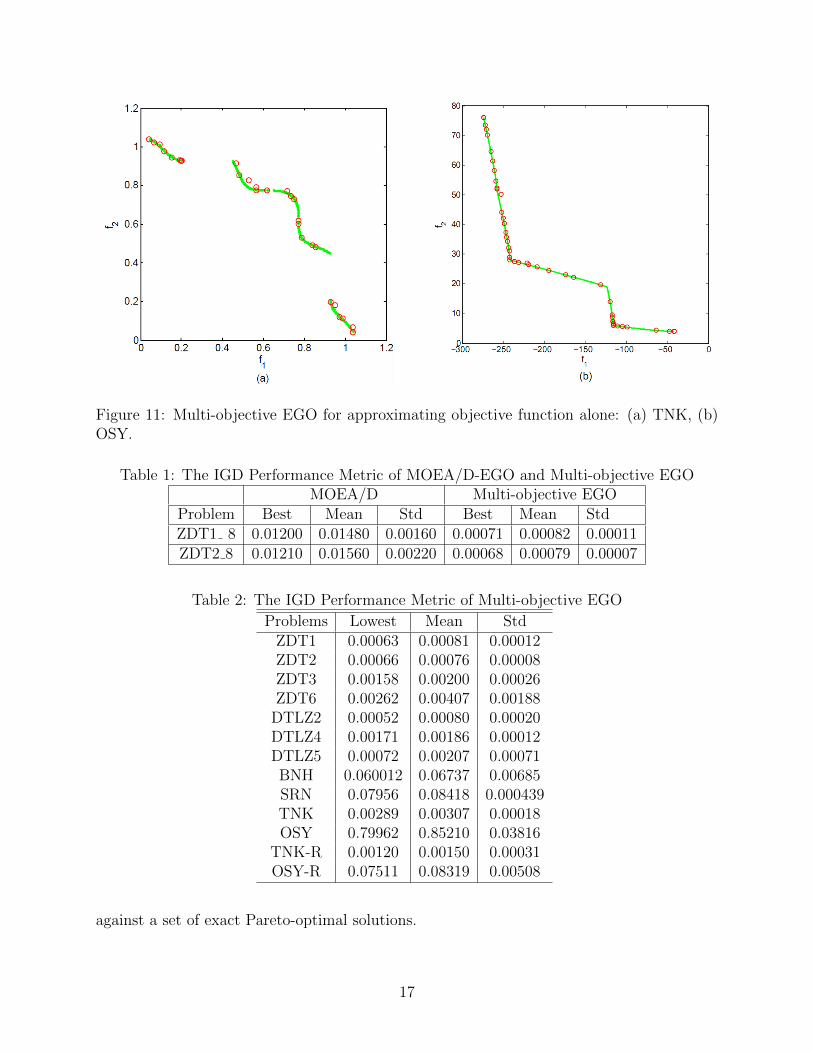
Figure 11: Multi-objective EGO for approximating objective function alone: (a) TNK, (b)OSY.

Table 1: The IGD Performance Metric of MOEA/D-EGO and Multi-objective EGOMOEA/D Multi-objective EGO

Problem Best Mean Std Best Mean StdZDT1 8 0.01200 0.01480 0.00160 0.00071 0.00082 0.00011ZDT2 8 0.01210 0.01560 0.00220 0.00068 0.00079 0.00007

Table 2: The IGD Performance Metric of Multi-objective EGO

Problems Lowest Mean StdZDT1 0.00063 0.00081 0.00012ZDT2 0.00066 0.00076 0.00008ZDT3 0.00158 0.00200 0.00026ZDT6 0.00262 0.00407 0.00188

DTLZ2 0.00052 0.00080 0.00020DTLZ4 0.00171 0.00186 0.00012DTLZ5 0.00072 0.00207 0.00071BNH 0.060012 0.06737 0.00685SRN 0.07956 0.08418 0.000439TNK 0.00289 0.00307 0.00018OSY 0.79962 0.85210 0.03816

TNK-R 0.00120 0.00150 0.00031OSY-R 0.07511 0.08319 0.00508

against a set of exact Pareto-optimal solutions.

17

5 Conclusions

Surrogate models are effective in reducing the computational time required to solve singleor multi-objective optimization problems. However, there has not been much studies inusing them for multi-objective optimization problems. The difficulty lies in finding a setof optimal solutions using one surrogate model, hence a common approach has been to usesingle-objective surrogate modeling approaches in a generative manner to find one solutionat a time.

In this work, we have proposed a generative surrogate modeling procedure for multi-objective optimization in which one model designed for finding a particular Pareto-optimalsolution helps in modeling and finding another neighboring Pareto-optimal solution. Ourproposed method is generic and is now ready to be tested for other surrogate modelingapproaches and for different sequence of building individual models. Our extensive simulationresults are compared with an existing study which was limited to small-sized problems. Ithas been observed that our approach can find a well converged and well diverged set ofsolutions on the originally proposed large-sized version of the test problems in a few hundredsof solution evaluations. Another hallmark of our approach is that we have proposed aconstrained handling method within the surrogate modeling approach that can solve difficultconstrained test problems of the multi-objective optimization literature.

We are now extending the proposed approach in many ways: (i) effect of other referencedirection sequencing approaches, (ii) effect of other surrogate modeling approaches, suchas radial basis neural network and SVM procedures, (iii) application to more complex testproblems and practical problems, and (iv) other non-generative, and multi-modal surrogatemodeling approaches. Results from these studies will be communicated as they are obtained.

References

[1] A. Forrester, A. Sobester, and A. Keane, Engineering design via surrogate modelling: Apractical guide. John Wiley & Sons, 2008.

[2] Q. Zhang, W. Liu, E. Tsang, and B. Virginas, “Expensive multiobjective optimizationby MOEA/D with gaussian process model,” vol. 14, no. 3, pp. 456–474, 2010-06.

[3] K. Shimoyama, K. Sato, S. Jeong, and S. Obayashi, “Updating Kriging surrogate modelsbased on the hypervolume indicator in multi-objective optimization,” vol. 135, 2013.

[4] D. R. Jones, “A taxonomy of global optimization methods based on response surfaces,”Journal of global optimization, vol. 21, no. 4, pp. 345–383, 2001.

[5] M. Emmerich, K. Giannakoglou, and B. Naujoks, “Single- and multiobjective evolution-ary optimization assisted by gaussian random field metamodels,” vol. 10, pp. 421–439,2006-08.

[6] D. Krige, “A statistical approach to some basic mine valuation problems on the Wit-watersrand,” Journal of the Chemical, Metallurgical and Mining Engineering Society ofSouth Africa, pp. 119–139, 1951.

18

[7] G. Matheron, “Principles of geostatistics,” Economic Geology, pp. 1246–1266, 1963.

[8] J. Sacks, W. J. Welch, T. J. Mitchell, and H. P. Wynn, “Design and analysis of computerexperiments,” Statistical science, pp. 409–423, 1989.

[9] S. N. Lophaven, H. B. Nielsen, and J. Søndergaard, “DACE–A Matlab Kriging toolbox,version 2.0,” Tech. Rep., 2002.

[10] D. R. Jones, M. Schonlau, and W. J. Welch, “Efficient global optimization of expensiveblack-box functions,” J. of Global Optimization, vol. 13, no. 4, pp. 455–492, 1998.

[11] Y. Jin, M. Olhofer, and B. Sendhoff, “A framework for evolutionary optimizationwith approximate fitness functions,” Evolutionary Computation, IEEE Transactionson, vol. 6, no. 5, pp. 481–494, 2002.

[12] C. C. Tutum, K. Deb, and I. Baran, “Constrained efficient global optimization forpultrusion process,” Materials and manufacturing processes, vol. 30, no. 4, pp. 538–551,2015.

[13] J. Knowles, “Parego: A hybrid algorithm with on-line landscape approximation forexpensive multiobjective optimization problems,” IEEE Trans. Evol. Comput., vol. 10,no.1, pp. 50–66, 2006.

[14] W. Ponweiser, T. Wagner, D. Biermann, and M. Vincze, “Multiobjective optimizationon a limited budget of evaluations using model–assisted S–metric selection,” in ParallelProblem Solving from Nature–PPSN X. Springer, 2008, pp. 784–794.

[15] Q. Zhang and H. Li, “MOEA/D : A multiobjective evolutionary algorithm based ondecomposition,” vol. 11, no. 6, pp. 712–731, 2007.

[16] K. Deb, “Multi-objective genetic algorithms: Problem difficulties and construction oftest problems,” Evolutionary computation, vol. 7, no. 3, pp. 205–230, 1999.

[17] I. Das and J. E. Dennis, “Normal-boundary intersection: A new method for generat-ing the pareto surface in nonlinear multicriteria optimization problems,” SIAM J. onOptimization, vol. 8, no. 3, 1998.

[18] A. P. Wierzbicki, “The use of reference objectives in multiobjective optimization,” inMultiple criteria decision making theory and application. Springer, 1980, pp. 468–486.

[19] K. Miettinen, Nonlinear multiobjective optimization. Springer Science & Business Me-dia, 2012, vol. 12.

[20] K. Deb, Multi-objective optimization using evolutionary algorithms. John Wiley &Sons, 2001, vol. 16.

[21] ——, “An efficient constraint handling method for genetic algorithms,” Computer meth-ods in applied mechanics and engineering, vol. 186, no. 2, pp. 311–338, 2000.

19

[22] K. Deb and A. Kumar, “Real-coded genetic algorithms with simulated binary crossover:studies on multimodal and multiobjective problems,” Complex Systems, vol. 9, no. 6,pp. 431–454, 1995.

20