a generalized discrete strong discontinuity approachframcos.org/framcos-7/02-07.pdf · a...

Fracture Mechanics of Concrete and Concrete Structures -Recent Advances in Fracture Mechanics of Concrete - B. H. Oh, et al.(eds)

2010 Korea Concrete Institute, Seoul, ISBN 978-89-5708-180-8

A generalized discrete strong discontinuity approach

D. Dias-da-Costa ISISE, Civil Engineering Department, University of Coimbra, Coimbra, Portugal

J. Alfaiate IST and ICIST, Civil Engineering Department, Instituto Superior Técnico, Lisboa, Portugal

L.J. Sluys Civil Engineering and Geosciences Department, Delft University of Technology, Delft, The Netherlands

E. Júlio ISISE, Civil Engineering Department, University of Coimbra, Coimbra, Portugal

ABSTRACT: Several local embedded discontinuity formulations have already been developed, in which con-stant strain triangles and constant jumps are adopted. However, these formulations lead to jump and traction discontinuity across element boundaries and stress locking effects. Herein, a new contribution to embedded strong discontinuities is given. A generalized discrete strong discontinuity approach (GSDA) is presented, in which non-homogeneous jumps can be embedded in any type of parent finite elements. A comparison to the generalized finite element method (GFEM) is also established. With this new formulation the additional de-grees of freedom are global and continuous jumps and tractions across the element boundaries are always ob-tained. The kinematics of the GSDA accurately reproduces both rigid-body motion and stretching induced by the opening of a discontinuity. Some simple examples are presented to illustrate the ability of this formulation in reproducing different opening modes. Structural examples, involving both mode-I and mixed-mode frac-ture, are also simulated and compared to experimental results.

1 INTRODUCTION

The numerical modeling of fracture behavior of quasi-brittle materials still poses important chal-lenges. Before a true crack is formed, microcracking extends over a significant area ahead of the crack tip, rendering the traditional assumptions of linear elastic fracture cumbersome.

The cohesive crack model proposed by Hiller-borg, Modeer et al. (1976) allowed for the simula-tion of discrete cracking. Initially, zero-thickness in-terface elements were applied. However, only after the development of finite elements with strong em-bedded discontinuities, a more efficient modeling of strain localization problems could be achieved. Most existing formulations (Dvorkin, Cuitiño et al. 1990, Simo & Rifai 1990, Klisinski, Runesson et al. 1991, Lofti & Shing 1995, Armero & Garikipati 1996, Larsson & Runesson 1996, Oliver 1996, Wells & Sluys 2001, Oliver, Huespe et al. 2002) take advan-tage of a static condensation, at element level, in or-der to keep the number of degrees of freedom con-stant. As a consequence, a discontinuous jump profile across element boundaries is obtained. More-over, constant strain triangles (CST) enriched with

constant jumps are usually applied, leading to well-known stress locking problems (Jirásek 2000).

In the embedded formulations introduced by Bol-zon (2001) and Linder & Armero (2007) linear dis-placement jumps at the discontinuity are adopted. However, the traditional CST elements are still used in the former case, whereas a local formulation is applied for both cases. In Dias-da-Costa, Alfaiate et al. (2009), a global formulation is presented, in which a non-homogeneous jump displacement field is considered across the discontinuity. These dis-placement jumps are transmitted to the parent ele-ment nodes by means of a rigid body motion. As a consequence, constant shear jumps are enforced, thus neglecting the stretching induced by the open-ing of a discontinuity.

Recently, the generalized finite element method (GFEM), also known as extended finite element me-thod (XFEM), became a powerful numerical tool available for the simulation of discontinuities (Duarte & Oden 1995, Melenk & Babuska 1996, Be-lytschko & Black 1999, Moës, Dolbow et al. 1999, Duarte, Babuska et al. 2000). This is a nodal en-richment technique, in which the partition of unity

property of the shape functions is exploited to ap-proximate the strong discontinuity kinematics.

In this paper, a generalized strong discontinuity approach (GSDA) is presented and compared to the GFEM method. Conversely to previous embedded formulations (Alfaiate, Simone et al. 2003, Dias-da-Costa, Alfaiate et al. 2009), all available degrees of freedom at the discontinuity are taken into account in order to capture both rigid body motion and stretching. This formulation can be applied to any parent element. Moreover, the additional degrees of freedom are global, meaning that the discontinuity jumps and tractions are kept continuous across ele-ment boundaries.

In Section 2 the problem description is presented, including the variational framework (Section 2.1), which is the same for the GSDA and the GFEM. The discretization of the variational equations is per-formed in Section 2.2. Some issues related to the numerical implementation are briefly reviewed in Section 3. The constitutive relation used in the com-puted examples is presented in Section 4. In Sec-tion 5.1 simple examples are computed in order to reveal particular aspects connected to the kinematics of both numerical techniques. Next, in Section 5.2, two structural examples are presented, one including mixed-mode fracture. Finally, in Section 6, the most relevant conclusions are presented.

2 PROBLEM DESCRIPTION

2.1 Common framework

In this Section the kinematics of a strong discontinu-ity is briefly addressed. More detail can be found elsewhere (see, for instance, Dias-da-Costa, Alfaiate et al. (2009)).

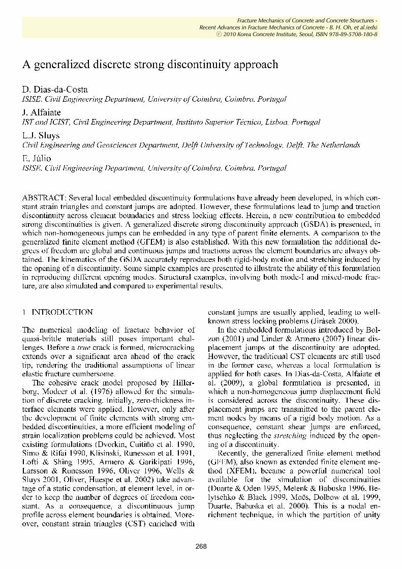
Consider an elastic domain Ω , with boundary Γ , containing a discontinuity surface

dΓ defining

two subregions +

Ω and −

Ω , according to Figure 1. A quasi-static loading composed by body forces,

b , and natural boundary conditions, t , the latter distributed on the external boundary,

tΓ , are ap-

plied to the body. The essential boundary conditions u distributed on the remaining part of the bound-ary,

uΓ , such that

t uΓ ∪Γ = Γ and

t uΓ ∩Γ =∅ .

The vector n is orthogonal to the boundary sur-face, pointing outwards, whereas +

n is orthogonal to the internal discontinuity surface, pointing in-wards +

Ω (see Fig. 1). The total displacement u is decomposed ac-

cording to the following equation:

ˆ( ) ( ) ( ),dΓ

= +u x u x u x%H (1)

where u represents the regular displacement field and u% is the enhanced displacement field.

dΓH is

a function defining the jump transmission by the dis-continuity. Here, the standard Heaviside function is chosen.

The strain field is defined, under small displace-ments hypothesis, as the symmetric part of the gra-dient of the displacement field:

( )s s s

unbounded

ˆ in ,d d

s

bounded

δΓ Γ

= ∇ = ∇ + ∇ + ⊗ Ωε u u u u n%1442443 1442443

H (2)

where (·)

s

stands for the symmetric part of (·) and ⊗ denotes the dyadic product.

Both displacement and strain fields remain con-tinuous in −

Ω and +

Ω , since the unbounded term in Equation (2) vanishes in

d

− +

Ω Γ = Ω ∪Ω .

u

n+

ΓdΓu

Ω− Ω+

nt

Γ

Γt

[[u]]

u|Γd= [[u]] u + u

Figure 1. Domain Ω crossed by a discontinuity surface

dΓ .

Under quasi-static equilibrium conditions, the

variational formulation can be cast into the follow-ing form:

( ) ( )s

\

\

ˆ :

ˆ ˆ· ·

d

d t

d

d d

Ω Γ

Ω Γ Γ

∇ Ω =

= Ω+ Γ

∫

∫ ∫

δ

δ δ

u σ ε

u b u t

(3)

and

( ) ( ) s

:

· · ,

d

t

d d

d d

+

+ +

+

Ω Γ

Ω Γ

∇ Ω+ Γ =

= Ω+ Γ

∫ ∫

∫ ∫

%

% %

δ δ

δ δ

u σ ε u t

u b u t

(4)

where ˆδu and δu% are, respectively, the regular and enhanced virtual displacements.

Both GSDA and GFEM formulations share the same variational framework defined by Equation (3) and (4). However, the GSDA remains an element enrichment technique, whereas the GFEM is a nodal enrichment technique. Therefore, discretization is addressed sepa-rately in the following subsection.

Proceedings of FraMCoS-7, May 23-28, 2010

hThD ∇−= ),(J (1)

The proportionality coefficient D(h,T) is called moisture permeability and it is a nonlinear function of the relative humidity h and temperature T (Bažant & Najjar 1972). The moisture mass balance requires that the variation in time of the water mass per unit volume of concrete (water content w) be equal to the divergence of the moisture flux J

J•∇=∂

∂−

t

w (2)

The water content w can be expressed as the sum

of the evaporable water we (capillary water, water vapor, and adsorbed water) and the non-evaporable (chemically bound) water wn (Mills 1966, Pantazopoulo & Mills 1995). It is reasonable to assume that the evaporable water is a function of relative humidity, h, degree of hydration, αc, and degree of silica fume reaction, αs, i.e. we=we(h,αc,αs) = age-dependent sorption/desorption isotherm (Norling Mjonell 1997). Under this assumption and by substituting Equation 1 into Equation 2 one obtains

nscw

s

ew

c

ew

hh

Dt

h

h

ew

&&& ++∂

∂

∂

∂

=∇•∇+∂

∂

∂

∂

− αα

αα

)(

(3)

where ∂we/∂h is the slope of the sorption/desorption isotherm (also called moisture capacity). The governing equation (Equation 3) must be completed by appropriate boundary and initial conditions.

The relation between the amount of evaporable water and relative humidity is called ‘‘adsorption isotherm” if measured with increasing relativity humidity and ‘‘desorption isotherm” in the opposite case. Neglecting their difference (Xi et al. 1994), in the following, ‘‘sorption isotherm” will be used with reference to both sorption and desorption conditions. By the way, if the hysteresis of the moisture isotherm would be taken into account, two different relation, evaporable water vs relative humidity, must be used according to the sign of the variation of the relativity humidity. The shape of the sorption isotherm for HPC is influenced by many parameters, especially those that influence extent and rate of the chemical reactions and, in turn, determine pore structure and pore size distribution (water-to-cement ratio, cement chemical composition, SF content, curing time and method, temperature, mix additives, etc.). In the literature various formulations can be found to describe the sorption isotherm of normal concrete (Xi et al. 1994). However, in the present paper the semi-empirical expression proposed by Norling Mjornell (1997) is adopted because it

explicitly accounts for the evolution of hydration reaction and SF content. This sorption isotherm reads

( ) ( )( )

( ) ( )⎥⎥

⎦

⎤

⎢⎢

⎣

⎡

⎥⎥⎥

⎦

⎤

⎢⎢⎢

⎣

⎡

−

−∞

+

−∞

−=

1110

,1

110

11,

1,,

hcc

ge

scK

hcc

ge

scG

sch

ew

αα

αα

αα

αααα

(4)

where the first term (gel isotherm) represents the physically bound (adsorbed) water and the second term (capillary isotherm) represents the capillary water. This expression is valid only for low content of SF. The coefficient G1 represents the amount of water per unit volume held in the gel pores at 100% relative humidity, and it can be expressed (Norling Mjornell 1997) as

( ) ss

s

vgkc

c

c

vgk

scG αααα +=,1

(5)

where k

cvg and k

svg are material parameters. From the

maximum amount of water per unit volume that can fill all pores (both capillary pores and gel pores), one can calculate K1 as one obtains

( )1

110

110

11

22.0188.00

,1

−⎟⎠

⎞⎜⎝

⎛−∞

⎥⎥⎥

⎦

⎤

⎢⎢⎢

⎣

⎡⎟⎠

⎞⎜⎝

⎛−∞

−−+−

=

hcc

ge

hcc

geGs

ssc

w

scK

αα

αα

αα

αα

(6)

The material parameters k

cvg and k

svg and g1 can

be calibrated by fitting experimental data relevant to free (evaporable) water content in concrete at various ages (Di Luzio & Cusatis 2009b).

2.2 Temperature evolution

Note that, at early age, since the chemical reactions associated with cement hydration and SF reaction are exothermic, the temperature field is not uniform for non-adiabatic systems even if the environmental temperature is constant. Heat conduction can be described in concrete, at least for temperature not exceeding 100°C (Bažant & Kaplan 1996), by Fourier’s law, which reads

T∇−= λq (7)

where q is the heat flux, T is the absolute temperature, and λ is the heat conductivity; in this

2.2 Discretization

In this section the discretized equations for both formulations are presented.

2.2.1 GSDA

The displacement field within each enriched element domain, e

Ω , can be cast in the following form:

( )( ) if ,d d

e e e e e e

dΓ Γ⎡ ⎤⎣ ⎦

= + − ∈Ω Γu N x a I H a x%H (5)

[ ]( ) at , e e e e

w ds= Γu N x w (6)

where e

N contains the element shape functions, e

a are the total nodal displacements, e

a% are the enhanced nodal displacements, I is a (2 2 )n n× identity matrix and

d

e

ΓH is a (2 2 )n n× diagonal

matrix composed by successively evaluating the Heaviside function at each of the 2n degrees of freedom of the finite element. e

wN is a ( )

wd n× ,

( 2d = in 2D and 3d = in 3D), matrix containing the shape functions used to approximate the jumps

e

u , which are reflected by degrees of freedom e

w measured at the

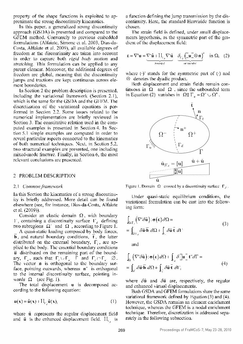
wn additional nodes, and ( )s x is

the coordinate along the discontinuity defined by Figure 2.

wn is related to the degree used to ap-

proximate the jumps: two additional nodes along

dΓ are used for a linear function (nodes i and j from Figure 2).

n

s

de+e

e−

Figure 2. Domain e

Ω crossed by a discontinuity surface e

dΓ .

The enhanced nodal displacements are obtained from:

,

e ek e

w=a M w% (7)

where ek

wM is a matrix transmitting the jumps to

the nodes of the enriched finite element. This matrix is formed by stacking, in rows, a matrix e

wM evalu-

ated at each node of the element. e

wM is decom-

posed into two matrices containing: (i) a linear shear slide, e

ws

M ; and (2) a rigid body rotation and trans-lation normal to the discontinuity, e

wn

M :

,

e e e

w= +

w ws n

M M M (8)

with

( ) ( ) ( )

( ) ( ) ( )

1 1 2 1 2 1 2 21

,2

1 2 1 1 2 2 1 2

e e e es c a s s a s c a s s an n n n

e e e es s a s c a s s a s c an n n n

e

⎡ ⎤⎛ ⎞ ⎛ ⎞− + − +⎜ ⎟ ⎜ ⎟⎢ ⎥⎝ ⎠ ⎝ ⎠⎢ ⎥=⎢ ⎥⎛ ⎞ ⎛ ⎞− − − −⎜ ⎟ ⎜ ⎟⎢ ⎥⎝ ⎠ ⎝ ⎠⎣ ⎦

w

Ms (9)

2 2 2 22 2 2 21 2 2

2 2

.

1 1 1 11 1 1 12 1 2

2 2

i i i ix x sa x x ca x x sa x x ca

c a s a

e e e el l l ld d d d

i i i ix x sa x x ca x x sa x x ca

s a c a

e e e el l l ld d d d

e

⎡ ⎤⎛ ⎞ ⎛ ⎞ ⎛ ⎞ ⎛ ⎞− − − −⎜ ⎟ ⎜ ⎟ ⎜ ⎟ ⎜ ⎟⎢ ⎥− ⎝ ⎠ ⎝ ⎠ ⎝ ⎠ ⎝ ⎠− − + −⎢ ⎥⎢ ⎥⎢ ⎥=⎢ ⎥⎛ ⎞ ⎛ ⎞ ⎛ ⎞ ⎛ ⎞− − − −⎜ ⎟ ⎜ ⎟ ⎜ ⎟ ⎜ ⎟⎢ ⎥+⎝ ⎠ ⎝ ⎠ ⎝ ⎠ ⎝ ⎠⎢ ⎥− + − −⎢ ⎥⎣ ⎦

w

Mn

(10)

In Equation (9) and (10), sin( )sa α= , cos( )ca α= ,

2 sin(2 )s a α= , 2 cos(2 )c a α= , and:

1 1 2 2

( ) cos( ) sin( )( ) ( ) ,e i ii

n e e e

d d d

ss x x x x

l l l

α α

= = − + −x

(11)

( )1 2,=x x x is the global position of any material

point inside the finite element, ( )1 2,

i i i=x x x is the

global position of the tip i , e

dl is the length of the

discontinuity e

dΓ measured along the local frame

s and α is the discontinuity angle (see Fig. 2). The strain field is approximated using the stan-

dard strain-displacement matrix, e

B :

( )( ) .d d

e e e e e

Γ Γ⎡ ⎤= + −⎣ ⎦

B x a I aε H %H (12)

The incremental stress field and incremental trac-

tion at the discontinuity are given by:

( )[ ],d d

e e e e e e

d d dΓ Γ

= + −σ D B a I H a%H (13)

at ,ee e e e e e

w dd d d= = Γt T u T N w (14)

where e

T is the discontinuity constitutive matrix. Taking into account Equation (5) into (14), the

descritization of Equation (3) and (4) leads to the following system of equations:

ˆ ,

e e e e e

aa awd d d+ =K a K w f (15)

( ) ,

e e e e e e

wa ww d wd d d+ + =K a K K w f (16)

with e e

d

e eT e e

aad

Ω Γ

= Ω∫K B D B

, e

aw=K

e e

d

eT e e e

wd

Ω Γ

= Ω∫ B D B ,

e e

d

e eT e e e

wa wd

Ω Γ

= Ω∫K B D B

,

e e

d

e eT e e e

ww w wd

Ω Γ

= Ω∫K B D B

, e

d

e e T e e

d w wd

Γ

= Γ∫K N T N ,

e e ek

w w=B B M , ( )

d d

ek e ek

w wΓ Γ= −I H MHM ,

\

ˆ

e e e

d t

ee eT eT e

d d dΩ Γ Γ

= Ω+ Γ∫ ∫f N b N t and

e e

t

e ee ekT eT ekT eT

w w wd d d

Ω Γ

= Ω+ Γ∫ ∫f N b N tM M .


hThD ∇−= ),(J (1)


J•∇=∂

∂−

t

w (2)



nscw

s

ew

c

ew

hh

Dt

h

h

ew

&&& ++∂

∂

∂

∂

=∇•∇+∂

∂

∂

∂

− αα

αα

)(

(3)




( ) ( )( )

( ) ( )⎥⎥

⎦

⎤

⎢⎢

⎣

⎡

⎥⎥⎥

⎦

⎤

⎢⎢⎢

⎣

⎡

−

−∞

+

−∞

−=

1110

,1

110

11,

1,,

hcc

ge

scK

hcc

ge

scG

sch

ew

αα

αα

αα

αααα

(4)


( ) ss

s

vgkc

c

c

vgk

scG αααα +=,1

(5)

where k

cvg and k



( )1

110

110

11

22.0188.00

,1

−⎟⎠

⎞⎜⎝

⎛−∞

⎥⎥⎥

⎦

⎤

⎢⎢⎢

⎣

⎡⎟⎠

⎞⎜⎝

⎛−∞

−−+−

=

hcc

ge

hcc

geGs

ssc

w

scK

αα

αα

αα

αα

(6)


cvg and k

svg and g1 can




T∇−= λq (7)


The additional degrees of freedom are considered global; as a consequence, both jump and traction continuity are obtained across elements. Traction continuity is enforced in the weak sense. Therefore, the symmetry is kept if the constitutive material law is symmetric.

2.2.2 GFEM

The derivation of the discretized equations for the GFEM is well known and therefore omitted. The corresponding system of equations is:

ˆ ˆ ˆ

ˆ

ˆ ,e e e e e

aa aad d d+ =

%

%K a K a f (17)

( )ˆ

ˆ ,e e e e e e

aa aa dd d d+ + =K a K K a f

% % %

%

% (18)

whereˆ ˆ e e

d

e eT e e

aad

Ω Γ

= Ω∫K B D B

,ˆ

e

aa=K

%

e

eT e e ed

+Ω

= Ω∫ B D B ,ˆ ˆ

e e eT

aa aa aa= =

% % % %

K K K , e

d=K

e

d

eT e ed

Γ

= Γ∫ N T N , ˆ

e

e eT ed d d

Ω

= Ω+∫f N b

,e

t

eT ed d

Γ

+ Γ∫ N te e

t

e eT e eT ed d d d d

+ +Ω Γ

= Ω+ Γ∫ ∫f N b N t%

3 NUMERICAL IMPLEMENTATION

3.1 Crack propagation technique

A discontinuity is considered straight, always cross-ing a complete parent element. Under crack propa-gation, additional degrees of freedom must be added to the GSDA and the GFEM. Only one discontinuity is allowed at each parent element, although generali-zations can be made for more than one (Daux, Moës et al. (2000); Dias-da-Costa, Alfaiate et al. (2009)).

The direction of crack propagation is evaluated applying Rankine criterion to an averaged stress ten-sor. A Gaussian weight function, presented in Wells & Sluys (2001) is used. This function depends on the distance between integration point and disconti-nuity tip and also on a significant distance around the tip, designated interaction radius. Different sug-gestions for the value for the radius of influence can be found (Wells & Sluys (2001); Simone (2003)). Here the value is defined as circa 1% of Hiller-borg’s characteristic length, 2

/ch F tl G E f= .

The stress field measured in the bulk is not lo-cally in equilibrium with the traction field measured in the discontinuity. This is a direct consequence of the weak traction continuity condition adopted in Equation (4). Consequently, at crack initiation, in order to prevent the traction field at the tip to lie out-side the limit surface, a conservative procedure is adopted: the discontinuities are introduced in an ear-

lier stage, in which the stress field in the bulk lies in-side the Rankine limit surface.

3.2 Numerical integration

In order to solve for the equilibrium equation pre-sented in Section 2.2, several numerical integrations need to be performed.

Regarding the integration of the discontinuity stiffness, e

dK , a two point Newton-Cotes/Lobatto

scheme is applied in the GSDA, in order to avoid spurious oscillations (Dias-da-Costa, Alfaiate et al. (2009)). Consequently, these integration points co-incide with the additional nodes located at the inter-section of the discontinuity with the element edges (Fig. 2).

With respect to the bulk stiffness, the subregion e+

Ω is divided in triangles defined by the centroid of e+

Ω and each edge surrounding e+

Ω . These tri-angular areas are afterwards integrated by a mid-point rule with three points. All remaining integrals, spanning over e

Ω , are computed by the usual Gaus-sian rule.

4 CONSTITUTIVE RELATIONS

In all examples presented in the following sections, the bulk is considered linear elastic. In the follow-ing, a brief review of the discontinuity traction-separation law is presented. A more comprehensive description, regarding plastic and damage models, can be found in Alfaiate, Wells et al. (2002); Dias-da-Costa, Alfaiate et al. (2009).

4.1 Isotropic damage law

The constitutive law for the isotropic damage law is given by:

(1 ) ,el

d= −t T w (19)

where d is a scalar damage variable such that 0 1d≤ ≤ and

elT is the initial elastic constitutive

tensor. The evolution of damage is written as:

0 0

0( ) 1 exp ( ) ,t

F

fd d

G

κ

κ κ κ

κ

⎛ ⎞= = − − −⎜ ⎟

⎝ ⎠ (20)

where

0tf is the initial tensile strength,

FG is the

fracture energy, and κ is a scalar equivalent jump damage parameter depending on the maximum ever reached positive normal jump component,

nw +

< > , and shear jump component, | |

sw :


hThD ∇−= ),(J (1)


J•∇=∂

∂−

t

w (2)



nscw

s

ew

c

ew

hh

Dt

h

h

ew

&&& ++∂

∂

∂

∂

=∇•∇+∂

∂

∂

∂

− αα

αα

)(

(3)




( ) ( )( )

( ) ( )⎥⎥

⎦

⎤

⎢⎢

⎣

⎡

⎥⎥⎥

⎦

⎤

⎢⎢⎢

⎣

⎡

−

−∞

+

−∞

−=

1110

,1

110

11,

1,,

hcc

ge

scK

hcc

ge

scG

sch

ew

αα

αα

αα

αααα

(4)


( ) ss

s

vgkc

c

c

vgk

scG αααα +=,1

(5)

where k

cvg and k



( )1

110

110

11

22.0188.00

,1

−⎟⎠

⎞⎜⎝

⎛−∞

⎥⎥⎥

⎦

⎤

⎢⎢⎢

⎣

⎡⎟⎠

⎞⎜⎝

⎛−∞

−−+−

=

hcc

ge

hcc

geGs

ssc

w

scK

αα

αα

αα

αα

(6)


cvg and k

svg and g1 can




T∇−= λq (7)


( ) max max | | .n sw wκ κ β+

= = < > +w (21)

β , which is always non-negative, defines the

contribution of the shear jump component to the equivalent jump parameter. At the onset of localization,

0sw = and 0

st = , whereas

0nw κ= and

0n tt f= .

A load function, in the displacement jump space, is defined as:

| | .n s

f w wβ κ+

=< > + − (22)

The incremental constitutive relation can be de-

rived from differentiation of Eq. (19):

(1 ) (1 ) ,el el el eld d d d= − − = − −t T w T w T w t& &

&

& & (23)

where el

t is the elastic traction vector and:

.

dd

κ

κ

∂ ∂=∂ ∂

w

w

&

& (24)

Finally, Eq. (23) can be cast into the following

form:

) . (1 el eldd

κ

κ

∂ ∂⎡ ⎤= − − ⊗⎢ ⎥∂ ∂⎣ ⎦

t T t ww

&

& (25)

If unloading takes place, the rate of damage is ze-

ro and the following relation is recovered:

(1 ) .eld= −t T w&

& (26)

5 NUMERICAL EXAMPLES

Some examples are computed to compare the per-formance of the GSDA and the GFEM. First, one element examples are presented for two different sit-uations: i) a discontinuity significantly softer than the bulk; and ii) vice-versa. Next, an example with stretching is also shown. Finally, two structural ex-amples are computed, the last of them including mixed-mode fracture. Plane stress state is assumed.

5.1 Simple examples

5.1.1 Soft discontinuity with rigid bulk vs. rigid dis-continuity with soft bulk

A horizontal discontinuity is placed at half the height of the parent element 3(1 1 1 mm )× × . A unit load is either vertically or horizontally applied at the top left node, to induce mode-I and mode-II crack opening, respectively. A linear elastic constitutive law is adopted for the discontinuity:

0,

0

se

n

k

k

⎡ ⎤= ⎢ ⎥⎣ ⎦

T (27)

Two situations are simulated: i) a soft discontinu-

ity ( 31 N/mm

nk = and 5 3

10 N/mms

k = , for mode-I; 5 3

10 N/mmn

k = and 31 N/mm

sk = , for mode-II) with

stiffer bulk ( 310 MPaE = ; 0ν = ); and ii) a stiffer

discontinuity ( 3 310 N/mm

nk = and 5 3

10 N/mms

k = , for mode-I; 5 3

10 N/mmn

k = and 3 310 N/mm

sk = ,

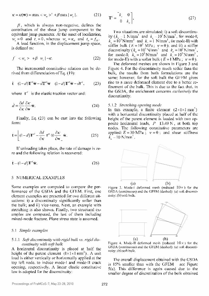
for mode-II) with a softer bulk ( 1 MPaE = ; 0ν = ). The deformed meshes are shown in Figure 3 and

Figure 4. For the discontinuity much softer than the bulk, the results from both formulations are the same; however, for the soft bulk the GFEM gives rise to a more deformed element due to a better re-finement of the bulk. This is due to the fact that, in the GSDA, the enrichment concerns exclusively the discontinuity.

5.1.2 Stretching opening mode In this example, a finite element 3(2 1 1 mm )× × with a horizontal discontinuity placed at half of the height of the parent element is loaded with two op-posite horizontal loads, 13.49 NP = , at both top nodes. The following constitutive parameters are applied: 30 MPaE = ; 0ν = ; and shear stiffness

310 N/mm

sk = .

(a) (b)

Figure 3. Mode-I deformed mesh (reduced 10× ) for the GSDA (continuous) and the GFEM (dashed): (a) soft disconti-nuity; (b) soft bulk.

(a) (b)

Figure 4. Mode-II deformed mesh (reduced 10× ) for the GSDA (continuous) and the GFEM (dashed): (a) soft disconti-nuity; (b) soft bulk.

The overall displacement obtained with the GSDA

is 15% smaller than with the GFEM – see Figure 5(a). This difference is again caused due to the smaller degree of discretization of the bulk obtained


hThD ∇−= ),(J (1)


J•∇=∂

∂−

t

w (2)



nscw

s

ew

c

ew

hh

Dt

h

h

ew

&&& ++∂

∂

∂

∂

=∇•∇+∂

∂

∂

∂

− αα

αα

)(

(3)




( ) ( )( )

( ) ( )⎥⎥

⎦

⎤

⎢⎢

⎣

⎡

⎥⎥⎥

⎦

⎤

⎢⎢⎢

⎣

⎡

−

−∞

+

−∞

−=

1110

,1

110

11,

1,,

hcc

ge

scK

hcc

ge

scG

sch

ew

αα

αα

αα

αααα

(4)


( ) ss

s

vgkc

c

c

vgk

scG αααα +=,1

(5)

where k

cvg and k



( )1

110

110

11

22.0188.00

,1

−⎟⎠

⎞⎜⎝

⎛−∞

⎥⎥⎥

⎦

⎤

⎢⎢⎢

⎣

⎡⎟⎠

⎞⎜⎝

⎛−∞

−−+−

=

hcc

ge

hcc

geGs

ssc

w

scK

αα

αα

αα

αα

(6)


cvg and k

svg and g1 can




T∇−= λq (7)


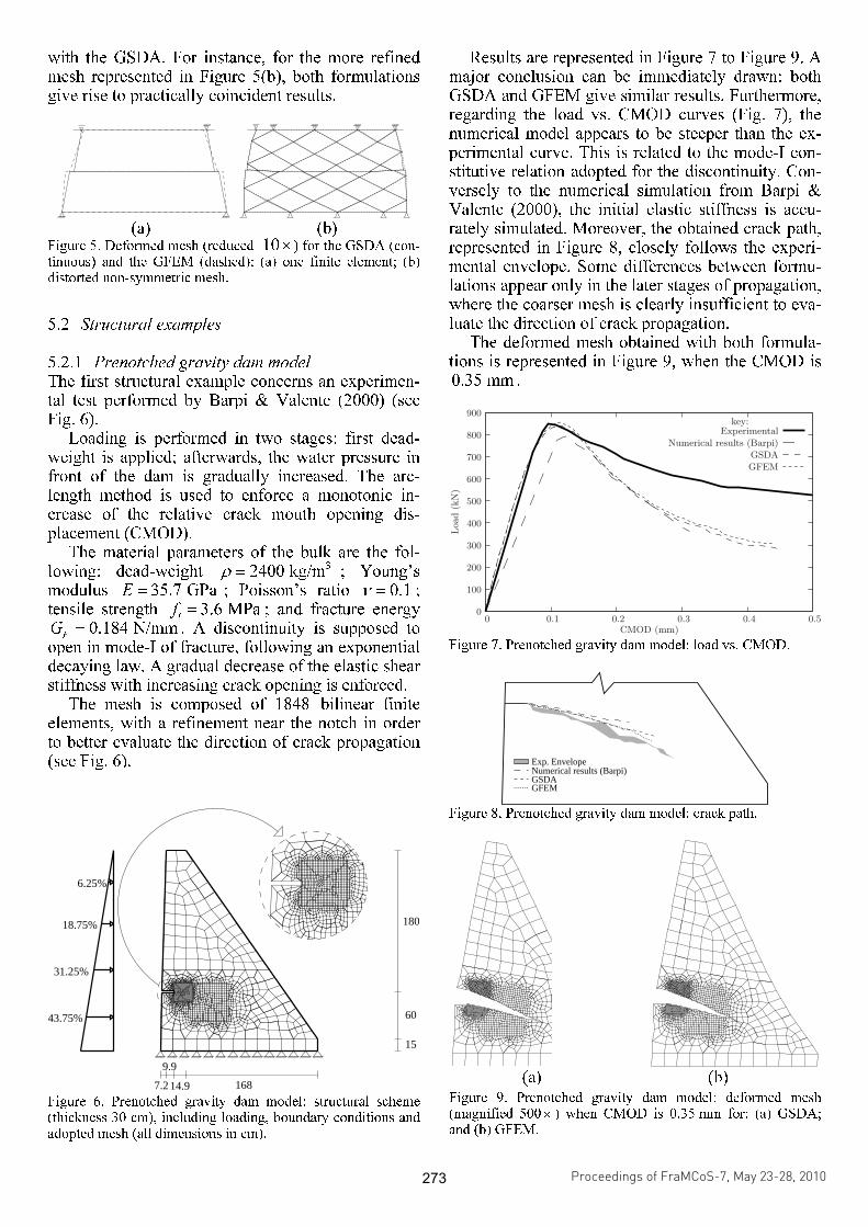
with the GSDA. For instance, for the more refined mesh represented in Figure 5(b), both formulations give rise to practically coincident results.

(a) (b)

Figure 5. Deformed mesh (reduced 10× ) for the GSDA (con-tinuous) and the GFEM (dashed): (a) one finite element; (b) distorted non-symmetric mesh.

5.2 Structural examples

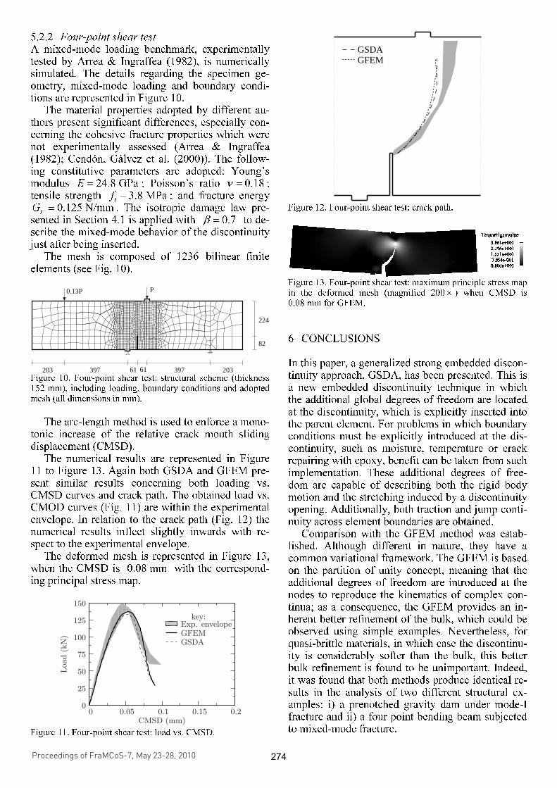
5.2.1 Prenotched gravity dam model The first structural example concerns an experimen-tal test performed by Barpi & Valente (2000) (see Fig. 6).

Loading is performed in two stages: first dead-weight is applied; afterwards, the water pressure in front of the dam is gradually increased. The arc-length method is used to enforce a monotonic in-crease of the relative crack mouth opening dis-placement (CMOD).

The material parameters of the bulk are the fol-lowing: dead-weight 32400 kg/mρ = ; Young’s modulus 35.7 GPaE = ; Poisson’s ratio 0.1ν = ; tensile strength 3.6 MPa

tf = ; and fracture energy

0.184 N/mmFG = . A discontinuity is supposed to open in mode-I of fracture, following an exponential decaying law. A gradual decrease of the elastic shear stiffness with increasing crack opening is enforced.

The mesh is composed of 1848 bilinear finite elements, with a refinement near the notch in order to better evaluate the direction of crack propagation (see Fig. 6).

43.75%

15

60

180

16814.97.2

9.9

6.25%

18.75%

31.25%

Figure 6. Prenotched gravity dam model: structural scheme (thickness 30 cm), including loading, boundary conditions and adopted mesh (all dimensions in cm).

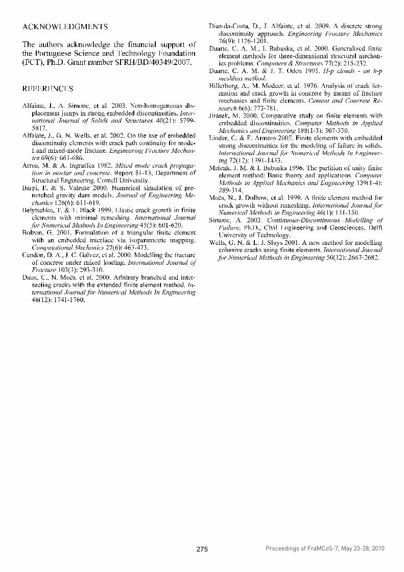
Results are represented in Figure 7 to Figure 9. A major conclusion can be immediately drawn: both GSDA and GFEM give similar results. Furthermore, regarding the load vs. CMOD curves (Fig. 7), the numerical model appears to be steeper than the ex-perimental curve. This is related to the mode-I con-stitutive relation adopted for the discontinuity. Con-versely to the numerical simulation from Barpi & Valente (2000), the initial elastic stiffness is accu-rately simulated. Moreover, the obtained crack path, represented in Figure 8, closely follows the experi-mental envelope. Some differences between formu-lations appear only in the later stages of propagation, where the coarser mesh is clearly insufficient to eva-luate the direction of crack propagation.

The deformed mesh obtained with both formula-tions is represented in Figure 9, when the CMOD is 0.35 mm .

GFEM

100

200

300

400

500

600

700

800

900

0 0.1 0.2 0.3 0.4 0.5

Load

(kN

)

CMOD (mm)

key:Experimental

Numerical results (Barpi)

GSDA

0

Figure 7. Prenotched gravity dam model: load vs. CMOD.

Exp. EnvelopeNumerical results (Barpi)GSDAGFEM

Figure 8. Prenotched gravity dam model: crack path.

(a) (b)

Figure 9. Prenotched gravity dam model: deformed mesh (magnified 500× ) when CMOD is 0.35 mm for: (a) GSDA; and (b) GFEM.


hThD ∇−= ),(J (1)


J•∇=∂

∂−

t

w (2)



nscw

s

ew

c

ew

hh

Dt

h

h

ew

&&& ++∂

∂

∂

∂

=∇•∇+∂

∂

∂

∂

− αα

αα

)(

(3)




( ) ( )( )

( ) ( )⎥⎥

⎦

⎤

⎢⎢

⎣

⎡

⎥⎥⎥

⎦

⎤

⎢⎢⎢

⎣

⎡

−

−∞

+

−∞

−=

1110

,1

110

11,

1,,

hcc

ge

scK

hcc

ge

scG

sch

ew

αα

αα

αα

αααα

(4)


( ) ss

s

vgkc

c

c

vgk

scG αααα +=,1

(5)

where k

cvg and k



( )1

110

110

11

22.0188.00

,1

−⎟⎠

⎞⎜⎝

⎛−∞

⎥⎥⎥

⎦

⎤

⎢⎢⎢

⎣

⎡⎟⎠

⎞⎜⎝

⎛−∞

−−+−

=

hcc

ge

hcc

geGs

ssc

w

scK

αα

αα

αα

αα

(6)


cvg and k

svg and g1 can




T∇−= λq (7)


5.2.2 Four-point shear test A mixed-mode loading benchmark, experimentally tested by Arrea & Ingraffea (1982), is numerically simulated. The details regarding the specimen ge-ometry, mixed-mode loading and boundary condi-tions are represented in Figure 10.

The material properties adopted by different au-thors present significant differences, especially con-cerning the cohesive fracture properties which were not experimentally assessed (Arrea & Ingraffea (1982); Cendón, Gálvez et al. (2000)). The follow-ing constitutive parameters are adopted: Young’s modulus 24.8 GPaE = ; Poisson’s ratio 0.18ν = ; tensile strength 3.8 MPa

tf = ; and fracture energy

0.125 N/mmFG = . The isotropic damage law pre-sented in Section 4.1 is applied with 0.7β = to de-scribe the mixed-mode behavior of the discontinuity just after being inserted.

The mesh is composed of 1236 bilinear finite elements (see Fig. 10).

224

82

397 61 39761 203203

P0.13P

Figure 10. Four-point shear test: structural scheme (thickness 152 mm), including loading, boundary conditions and adopted mesh (all dimensions in mm).

The arc-length method is used to enforce a mono-

tonic increase of the relative crack mouth sliding displacement (CMSD).

The numerical results are represented in Figure 11 to Figure 13. Again both GSDA and GFEM pre-sent similar results concerning both loading vs. CMSD curves and crack path. The obtained load vs. CMOD curves (Fig. 11) are within the experimental envelope. In relation to the crack path (Fig. 12) the numerical results inflect slightly inwards with re-spect to the experimental envelope.

The deformed mesh is represented in Figure 13, when the CMSD is 0.08 mm with the correspond-ing principal stress map.

GSDA

25

50

75

100

125

150

0 0.05 0.1 0.15 0.2

Load

(kN

)

CMSD (mm)

key:Exp. envelopeGFEM

0

Figure 11. Four-point shear test: load vs. CMSD.

GSDAGFEM

Figure 12. Four-point shear test: crack path.

Figure 13. Four-point shear test: maximum principle stress map in the deformed mesh (magnified 200 × ) when CMSD is 0.08 mm for GFEM.

6 CONCLUSIONS

In this paper, a generalized strong embedded discon-tinuity approach, GSDA, has been presented. This is a new embedded discontinuity technique in which the additional global degrees of freedom are located at the discontinuity, which is explicitly inserted into the parent element. For problems in which boundary conditions must be explicitly introduced at the dis-continuity, such as moisture, temperature or crack repairing with epoxy, benefit can be taken from such implementation. These additional degrees of free-dom are capable of describing both the rigid body motion and the stretching induced by a discontinuity opening. Additionally, both traction and jump conti-nuity across element boundaries are obtained.

Comparison with the GFEM method was estab-lished. Although different in nature, they have a common variational framework. The GFEM is based on the partition of unity concept, meaning that the additional degrees of freedom are introduced at the nodes to reproduce the kinematics of complex con-tinua; as a consequence, the GFEM provides an in-herent better refinement of the bulk, which could be observed using simple examples. Nevertheless, for quasi-brittle materials, in which case the discontinu-ity is considerably softer than the bulk, this better bulk refinement is found to be unimportant. Indeed, it was found that both methods produce identical re-sults in the analysis of two different structural ex-amples: i) a prenotched gravity dam under mode-I fracture and ii) a four point bending beam subjected to mixed-mode fracture.


hThD ∇−= ),(J (1)


J•∇=∂

∂−

t

w (2)



nscw

s

ew

c

ew

hh

Dt

h

h

ew

&&& ++∂

∂

∂

∂

=∇•∇+∂

∂

∂

∂

− αα

αα

)(

(3)




( ) ( )( )

( ) ( )⎥⎥

⎦

⎤

⎢⎢

⎣

⎡

⎥⎥⎥

⎦

⎤

⎢⎢⎢

⎣

⎡

−

−∞

+

−∞

−=

1110

,1

110

11,

1,,

hcc

ge

scK

hcc

ge

scG

sch

ew

αα

αα

αα

αααα

(4)


( ) ss

s

vgkc

c

c

vgk

scG αααα +=,1

(5)

where k

cvg and k



( )1

110

110

11

22.0188.00

,1

−⎟⎠

⎞⎜⎝

⎛−∞

⎥⎥⎥

⎦

⎤

⎢⎢⎢

⎣

⎡⎟⎠

⎞⎜⎝

⎛−∞

−−+−

=

hcc

ge

hcc

geGs

ssc

w

scK

αα

αα

αα

αα

(6)


cvg and k

svg and g1 can




T∇−= λq (7)


ACKNOWLEDGMENTS

The authors acknowledge the financial support of the Portuguese Science and Technology Foundation (FCT), Ph.D. Grant number SFRH/BD/40349/2007.

REFERENCES

Alfaiate, J., A. Simone, et al. 2003. Non-homogeneous dis-placement jumps in strong embedded discontinuities. Inter-national Journal of Solids and Structures 40(21): 5799-5817.

Alfaiate, J., G. N. Wells, et al. 2002. On the use of embedded discontinuity elements with crack path continuity for mode-I and mixed-mode fracture. Engineering Fracture Mechan-ics 69(6): 661-686.

Arrea, M. & A. Ingraffea 1982. Mixed mode crack propaga-tion in mortar and concrete. Report 81-13, Department of Structural Engineering, Cornell University.

Barpi, F. & S. Valente 2000. Numerical simulation of pre-notched gravity dam models. Journal of Engineering Me-chanics 126(6): 611-619.

Belytschko, T. & T. Black 1999. Elastic crack growth in finite elements with minimal remeshing. International Journal for Numerical Methods In Engineering 45(5): 601-620.

Bolzon, G. 2001. Formulation of a triangular finite element with an embedded interface via isoparametric mapping. Computational Mechanics 27(6): 463-473.

Cendón, D. A., J. C. Gálvez, et al. 2000. Modelling the fracture of concrete under mixed loading. International Journal of Fracture 103(3): 293-310.

Daux, C., N. Moës, et al. 2000. Arbitrary branched and inter-secting cracks with the extended finite element method. In-ternational Journal for Numerical Methods In Engineering 48(12): 1741-1760.

Dias-da-Costa, D., J. Alfaiate, et al. 2009. A discrete strong discontinuity approach. Engineering Fracture Mechanics 76(9): 1176-1201.

Duarte, C. A. M., I. Babuska, et al. 2000. Generalized finite element methods for three-dimensional structural mechan-ics problems. Computers & Structures 77(2): 215-232.

Duarte, C. A. M. & J. T. Oden 1995. H-p clouds - an h-p meshless method.

Hillerborg, A., M. Modeer, et al. 1976. Analysis of crack for-mation and crack growth in concrete by means of fracture mechanics and finite elements. Cement and Concrete Re-search 6(6): 773-781.

Jirásek, M. 2000. Comparative study on finite elements with embedded discontinuities. Computer Methods in Applied Mechanics and Engineering 188(1-3): 307-330.

Linder, C. & F. Armero 2007. Finite elements with embedded strong discontinuities for the modeling of failure in solids. International Journal for Numerical Methods In Engineer-ing 72(12): 1391-1433.

Melenk, J. M. & I. Babuska 1996. The partition of unity finite element method: Basic theory and applications. Computer Methods in Applied Mechanics and Engineering 139(1-4): 289-314.

Moës, N., J. Dolbow, et al. 1999. A finite element method for crack growth without remeshing. International Journal for Numerical Methods in Engineering 46(1): 131-150.

Simone, A. 2003. Continuous-Discontinuous Modelling of Failure. Ph.D., Civil Engineering and Geosciences, Delft University of Technology.

Wells, G. N. & L. J. Sluys 2001. A new method for modelling cohesive cracks using finite elements. International Journal for Numerical Methods in Engineering 50(12): 2667-2682.


hThD ∇−= ),(J (1)


J•∇=∂

∂−

t

w (2)



nscw

s

ew

c

ew

hh

Dt

h

h

ew

&&& ++∂

∂

∂

∂

=∇•∇+∂

∂

∂

∂

− αα

αα

)(

(3)




( ) ( )( )

( ) ( )⎥⎥

⎦

⎤

⎢⎢

⎣

⎡

⎥⎥⎥

⎦

⎤

⎢⎢⎢

⎣

⎡

−

−∞

+

−∞

−=

1110

,1

110

11,

1,,

hcc

ge

scK

hcc

ge

scG

sch

ew

αα

αα

αα

αααα

(4)


( ) ss

s

vgkc

c

c

vgk

scG αααα +=,1

(5)

where k

cvg and k



( )1

110

110

11

22.0188.00

,1

−⎟⎠

⎞⎜⎝

⎛−∞

⎥⎥⎥

⎦

⎤

⎢⎢⎢

⎣

⎡⎟⎠

⎞⎜⎝

⎛−∞

−−+−

=

hcc

ge

hcc

geGs

ssc

w

scK

αα

αα

αα

αα

(6)


cvg and k

svg and g1 can




T∇−= λq (7)


a generalized discrete strong discontinuity approachframcos.org/framcos-7/02-07.pdf · a...

Documents