A Generalized Cognitive Hierarchy Model of Games

Juin-Kuan Chong, Teck-Hua Ho, and Colin Camerer∗

June 4, 2014

Subjects in simple games often exhibit nonequilibrium behaviors. Cognitive Hierarchy (CH)

and Level k (LK) are two prevailing structural models that can predict these behaviors well

but they make quite different assumptions on players’ beliefs of their opponents’ actions.

This paper develops a generalization of CH and shows that CH and a variant of LK belong

to the same family. Under generalized CH (GCH), level k players best respond to level 0 to

level k−1 but the perceived proportion of each lower level is obtained by weighting its actual

frequency by a parameter α, reflecting stereotype bias well documented in social psychology

literature. When α = 1, GCH reduces to CH; and when α =∞, it becomes Level m (LM) in

which level k best responds to only the modal level below k (and the modal level may be k−1).

GCH also fixes prior ad-hoc assumptions about level 0 by developing a plausible model for

it. GCH posits that non-strategic level 0 players are more likely to choose strategies that will

never yield the minimum payoff in all possible outcome scenarios. This minimum-aversion

tendency captures level 0’s avoidance for dominated strategies and compromise effects well-

documented in the individual choice literature. Using fifty-five 2-player m x n games from

four distinct datasets, we show that GCH describes and predicts behaviors better than CH

and LK. Structural estimation results show that higher level players exhibit stereotype bias

and level 0 players exhibit minimum aversion. Finally, we apply GCH to two new games and

find that GCH is able to overcome CH’s inadequacies and predict behavior remarkably well.

Keywords: Cognitive Hierarchy, Level k Model, Level m Model, Generalized Cognitive Hi-

erarchy, Nonequilibrium Structural Models, Behavioral Game Theory

∗Chong: National University of Singapore. Ho: University of California, Berkeley and National University

of Singapore. Camerer: Caltech. Direct correspondence to Juin-Kuan Chong: bizcjk@nus.edu.sg. We thank

Vince Crawford for his encouragement and Sada Reza for his research assistance.

1

1 Introduction

Subjects frequently do not play equilibrium in simple one-shot games. Sometimes these

nonequilibrium behaviors persist even when subjects engage in repeated plays and when

they are motivated by substantial financial incentives. Both nonequlibrium phenomena pose

serious challenges for standard equilibrium models. Recent research has developed structural

nonequilibrium models as alternatives and these models have shown promise in explaining

and predicting these out-of-equilibrium behaviors in a wide variety of games and markets

(see Crawford (2013) for a comprehensive review).

Standard equilibrium models make three fundamental assumptions to generate their pre-

diction: 1) players form subjective beliefs about what their opponents will do, 2) players

choose actions to maximize their expected payoffs conditional on their belief (i.e., they are

subjective utility maximizers), and 3) players’ subjective beliefs are always correct (i.e., their

beliefs always match their opponents’ actual actions). The third assumption is particularly

strong because it uses opponents’ actual actions to pin down players’ beliefs. Since players’

beliefs are always correct under standard equilibrium models, no players will ever be sur-

prised by their opponents’ actions. Nonequilibrium structural models, on the other hand,

do not require players’ subjective beliefs to be always correct. As a result, players can be

surprised by their opponents’ actions in actual game plays (as we observe in many real-world

situations).

To generate their behavioral prediction, existing nonequilibrium models posit that players

are heterogenous and have different levels of thinking ability. The proportion of player with

thinking level k (k = 0, 1, . . . ,∞) is denoted by f(k). Clearly,∑∞

k=0 f(k) = 1. These models

starts with an explicit assumption on how non-strategic level 0 players behave. Higher level

players’ behaviors are then determined iteratively by assuming they best-respond to lower

level players. As a consequence, the aggregate behavioral prediction is simply an average of

each level’s behavior weighted by its actual proportion.

Cognitive Hierarchy (CH) (Camerer, Ho and Chong, 2004) and Level k (LK) (Nagel, 1995;

Stahl and Wilson, 1994, 1995; Costa-Gomes, Crawford and Broseta, 2001; Costa-Gomes and

Crawford, 2006) have been successful in explaining nonequilibrium behaviors, however, they

2

make quite different assumptions on how higher level players best respond to lower level

players. Both models start with a specification of level 0 rule. While LK assumes that level

k best-responds to only level k − 1, CH assumes that level k best respond to all lower level

(i.e., 0, 1, . . . , k − 2, k − 1) with the perceived proportion of each lower level equals to its

normalized true proportion (i.e., perceived proportion of level h = f(h)∑k−1h′=0

f(h′), for all h < k).

This paper develops a generalization of CH and shows that it nests a variant of LK, which

we call Level m (LM) model. Like LK, LM assumes each level of player best-responds to

only one lower level player. Unlike LK, however, LM assumes level k best-responds to the

most frequently occurring lower level (i.e. the modal level below k), reflecting stereotype

bias. If the modal level happens to be k− 1, LK and LM make the same prediction for level

k behavior.

Generalized Cognitive Hierarchy (GCH) assumes that level k best-responds to all lower levels

but the perceived proportion of each lower level is obtained by weighting its actual frequency

by a parameter α. Specifically, level k’s belief of the proportion of level h(< k), the perceived

proportion of level h, is equal to f(h)α∑k−1h′=0

f(h′)α. As a result, GCH reduces to CH when α = 1

and LM when α = ∞. Note that when α = ∞, perceived proportion of level h = 1 if

h = argmaxh′<k f(h′) and 0 otherwise. We shall show below that LM avoids an undesirable

property of LK, which predicts oscillating player behavior in some games including market

entry.

The behavioral prediction of non-equilibrium structural models depends critically on level

0’s behavioral rule because higher level rules are defined iteratively based on lower level

ones. Despite its importance, there is a lack of a plausible model for level 0’s rule that can

be applied uniformly to all games. Existing research uses two different models of level 0’s

rule. In one model, level 0 is assumed to randomize her choice uniformly across all possible

actions (e.g., Camerer et al, 2004). While the random choice rule is general, it appears too

naive as a plausible rule of behavior for actual players in practice. In another model, saliency

is used to derive level 0’s rule from the game structure (e.g., Crawford and Iriberri, 2007).

This saliency-based model, while plausible, can sometimes appear ad-hoc. This is so because

saliency is not precisely defined and different people may invoke a different saliency principle.

In this paper, we develop a model of level 0 that aims to address the inadequacies of existing

3

models of level 0. Our model hypothesizes that level 0 players use minimum avoidance as

the saliency principle in choosing their strategy. Specifically, they prefer strategies that will

not yield the minimum payoff in all possible outcome scenarios. Let’s illustrate the mini-

mum avoidance principle with a nxm game matrix. We focus on the row player i who has n

strategies. Strategy j belongs to the preferred set Si if strategy j never yields the minimum

payoff in any of the m possible opponent’s strategies. Our model posits that level 0 players

choose strategies in set Si β times more likely than those outside Si. As a consequence,

level 0 players choose each of the strategies in Si with probability βn−|Si|+|Si|·β and each of the

strategies not in Si with probability 1n−|Si|+|Si|·β , where |Si| is the cardinality of the set Si.

Below, we show that this simple model of level 0’s rule exhibits dominance and compromise

effects, two behavioral phenomena well-documented in the individual choice literature. In

addition, it predicts that level 0 is less likely to choose dominated strategies, which fixes a

weakness of the random choice model. Note that when β = 1, the model reduces to random

choice rule. When β =∞, level 0 never chooses strategies outside the preferred set Si.

GCH has 2 more parameters (i.e., α and β) than the CH model. The α parameter allows us

to investigate various models of opponents in a common framework. It allows us to establish

an explicit link between CH and a variant of LK (i.e., LM). The β parameter uses minimum

avoidance as the saliency principle and allows us to model random choice and saliency as

two extreme special cases of a well-defined model of level 0.

We fit GCH to 55 n x m games (with n,m = 2,3,4,5,6) from 4 distinct datasets. We show

that our generalized model describes and predict behaviors better than CH and LK models.

Both α and β are important and add to the overall fit. The parameter α is always greater

1, suggesting that higher level players exhibit stereotype bias. The parameter β is always

greater than 1, suggesting that level 0 players exhibit minimum aversion. We also estimate

nested cases of GCH and show that they are rejected in favor of the general model.

To check for robustness, we apply GCH to predict behavior in two new games. In all games,

CH did not predict the observed behaviors well. In the first game, Carrillo and Palfrey

(2009) find that people tend to fight in a fight-or-compromise game less frequently than

Nash equilibrium would predict. We show that GCH is able to overcome CH’s shortcomings

and predict observed behaviors remarkably well. In the second game, Amaldoss, Bettman

4

and Payne (2008) add an irrelevant (i.e., dominated) alternative to a coordination game and

show that subjects are better able to coordinate their behavior. GCH is able to capture the

better coordination.

The rest of the paper is organized as follows. Section 2 describes the model. It shows how

the GCH model nests CH and LM as special cases. Section 3 compares LM and LK models

in several games (including the entry game) and describes their similarities and differences.

It shows that LM does not exhibit oscillating behavior. Section 4 provides MLE estimates of

GCH, CH, LM, LK and a 2-parameter LK models. Section 5 describes two applications of

best fitted GCH to 2 new games. Section 6 concludes and suggests future research directions.

2 Model

2.1 Notations

We focus the GCH model on 2-player matrix games. Beginning with notation, we index

players by i and denote player i’s jth strategy by sji . Player i chooses from mi possible

strategies. Player i’s opponent is denoted by −i and her strategy profile by sj′

−i, and there

are m−i such strategies. Player i’s payoff is denoted by πi(sji , s

j′

−i). Players are heteroge-

nous and choose a rule from a rule hierarchy. We index rule levels in the rule hierarchy by k

(k = 0, 1, 2, . . . , k−1, k, . . . ,∞) and denote the proportion of level k players by f(k). Clearly∑∞k=0 f(k) = 1. In the empirical estimation, we assume f(.) follows a 1-parameter Poisson

distribution with mean and variance τ . Formally, f(k) = τk·e−k·τk!

.

2.2 Model of Opponent

Denote the probability that a player i with rule level k choosing strategy sji by Pk(sji ). Like

CH, GCH posits that level k best responds to level 0 to level k− 1 and chooses the strategy

that maximizes her expected payoff. The expected payoff of choosing sji is computed on

the basis of level k’s belief on what the lower levels will do. Denote the expected payoff of

strategy sji for level k as Ek(sji ). The expected payoff is computed as follows:

5

Ek(sji ) =

m−i∑j′=1

πi(sji , s

j′

−i){k−1∑h=0

gk(h) · Ph(sj′

−i)} (1)

where gk(h) is level k’s belief on the proportion of level h, h < k.

A level k player believes that the relative proportion of lower level h is:

gk(h) =f(h)α∑k−1i=0 f(i)α

, ∀h < k. (2)

The parameter α ≥ 1 captures the tendency of players exhibiting stereotype bias. When

α = 1, level k’s belief of lower level equals to its normalized true proportion and hence cor-

rectly reflecting the relative proportions of the lower levels. When α > 1, player k’s belief of

lower levels is concentrated on the more frequently occurring levels. This bias is the stereo-

type bias. Stereotype bias is well documented in social psychology literature. Stereotype

bias is a simplification of beliefs (where heterogeneity of outgroup members is reduced) when

people are faced with heavy cognitive load or when their cognitive resources are depleted.

This simplification of belief is done to achieve efficiency in information processing and deci-

sion making.

Note that when α = 1, GCH reduces to CH. When α =∞, level k exhibits extreme stereo-

type bias and believes that her opponent is only of the most frequently occurring lower rule.

We call this special case the Level m (LM), in contrast to LK, which places the entire weight

on level k−1. Both LK and LM assume that level k player believes that his opponent is of a

singular type; the type is level k−1 in LK and the modal lower rule in LM. If the modal rule

is always level k − 1, ∀k, then the two models are identical. For well-behaved single-modal

distributions (e.g., Poisson), the two models generate an identical prediction for level k up

to the mode+1 and a different prediction for level k above mode+1.

6

2.3 Model of Level 0

As discussed below, there are two existing models of level 0 rule. One model assumes that

level 0 uniformly randomizes among all possible strategies. This model has the advantage

that it is well-defined and general. However, it does not appear plausible for describing be-

haviors of sufficiently motivated subjects. The second model assumes that Level 0 chooses a

salient action in the feasible strategy space. This model receives the criticism of being ad-hoc

because it is often unclear ex ante which action is salient in some games. GCH addresses

the inadequacies of these models by proposing a model of level 0 that is both behaviorally

plausible and empirically general.

GCH assumes that level 0 players are averse to receiving minimum payoffs. Specifically, the

model assumes that level 0 is more likely to choose from a set of strategies that will never

yield the minimum payoff in any outcome scenario. That is, a strategy in this set will always

provide a strictly higher payoff than at least one other strategy in any outcome scenario.

These strategies are never the worst.

For player i, we define i’s “never worst set” Si as the the set of strategies that will never yield

the worst payoff in any of the possible strategies of opponent −i. Specifically, any strategy j

in set Si will yield a strictly higher payoff than at least one other strategy in every possible

strategy of −i. Formally, if i’s strategies are indexed by j as well as j′ and −i’s strategies

are indexed by j′′, then Si = {j : πi(sji , s

j′′

−i) > minj′{πi(sj′

i , sj′′

−i), ∀j′′}. GCH posits that

level 0 player i choose strategies in Si β times more likely those not in Si. Hence, the choice

probability of level 0 for each strategy sji is as follows:

P0(sji ) =

β

mi−|Si|+|Si|·β if j ∈ Si

1mi−|Si|+|Si|·β otherwise.

(3)

where |Si| is the cardinality of Si. Note that Si can be a null set and in this case our model

reduces to the uniform randomization rule with level 0 players choose each strategy with an

equal probability of 1mi

.

The proposed model of non-strategic level 0 captures two well-established empirical regular-

ities documented in the individual choice literature: 1) dominant strategies are chosen more

7

frequently than dominated strategies, and 2) compromise effects. In addition, the model also

captures the asymmetric dominance phenomena when the dominant strategy does not have

a minimum. The following three examples illustrate these phenomenas.

1. Existence of Dominant Strategies

When player i has 2 strategies and one of them is strictly dominant, level 0 player

chooses this strategy with probability of β1+β

. Table 1 shows one such game (Game

2 from Cooper and Van Huyck, 2003). The dominant strategy is labeled T, which

pays 0.4 and 0.6 when the opponent chooses L and R respectively. It is more than

what strategy B will pay in both scenario which is 0.2. GCH allows us to investigate

whether by allowing level 0 to choose T β times more likely than B would help to

describe and predict behaviors better in this kind of games. There are 10 games that

have a dominant strategy for at least one of the two players in the 55 games we studied.

Table 1: Game 2 from Cooper and Van Huyck [2003]

L R data

T .4,.5 .6,.3 .909

B .2, .1 .2, .1 .091

data .738 .262

Note: Payoffs in bold indicate the minimum payoff for the

corresponding columns or rows. The never worst set for

the row player consists of the dominant strategy T while

the never worst set for column player is empty.

2. Compromise Effects

Decision makers have a tendency to select a compromise alternative in individual

choice. Specifically, in a choice among three alternatives with 2 attributes, they often

prefer the alternative that yields intermediate payoffs in both attributes to alterna-

tives that yield high payoff in one attribute and low payoff in the other attribute. This

behavioral phenomenon of minimum aversion is called compromise effect. If players

exhibit compromise effect in games, they may choose a strategy that never yields the

8

minimum payoff. We use Game 10 from Camerer et al (2004) to illustrate this behav-

ioral tendency. Strategy M of row player is a compromise alternative because it gives

intermediate payoffs of -10 and 0 when the column player chooses L and R respec-

tively. It also gives the maximum payoff of 30 when column player chooses C. Note

that strategy M never receives the worst payoff in all possible outcome scenarios. GCH

predicts that level 0 chooses M with probability β2+β

and T or B with probability 12+β

.

Interestingly, subjects in this game play Strategy M with a frequency of 96%. In the

55 games we analyze, there are 10 games with such payoff structure.

Table 2: Game 10 from Camerer et al [2004]

L C R data

T -20,20 30,-30 -30,30 .00

M -10,10 30,30 0,0 .96

B 0,0 -10,10 10,-10 .04

data .29 .58 .13

Note: Payoffs in bold indicate the minimum payoff for the corre-

sponding columns or rows. The never worst set for the row player

consists of strategy M while the never worst set for column player

is strategy L.M is the compromise alternative which gives the in-

termediate payoff of -10 and 0 when opponent chooses L and R.

3. Asymmetric Dominance

Sometimes there is no dominant strategy in a 2x2 game. One way to make a strat-

egy more attractive is by adding a dominated strategy to the feasible strategy space.

Equilibrium models predict that players will not behave differently with the addition

of irrelevant alternative. However experimental literature suggests that players often

choose the strategy that dominates the added (and dominated) strategy more fre-

quently. We use Game 6 from Costa Gomes et al (2001) to illustrate this phenomenon.

This game is a 3x2 matrix game with payoff matrix as shown in Table 3. Note that

strategy M is a dominated strategy (it is dominated by B). If players exhibit asymmet-

ric dominance, they will be more likely to choose strategy B. Indeed, B is played 75%

of the time by the row players even though this game has a unique pure strategy Nash

9

equilibrium at (T,L). GCH can capture this phenomenon since its level 0 chooses B

with probability β2+β

and strategy T and M with probability 12+β

. There were 7 games

with asymmetric dominance payoff structure for at least of one of the two players in

the 55 games we studied.

Table 3: Game 6 from Costa Gomes et al [2001]

L R data

T 74,62 43,40 .14

M 25,12 76,93 .11

B 59,37 94,16 .75

data .70 .30

Note: Payoffs in bold indicate the minimum payoff for

the corresponding columns or rows. The never worst set

for the row player consists of strategy B which domi-

nates strategy M. The never worst set for column player

is empty.

In sections 4 and 5, we provide precise measure of statistical significance for the GCH model.

Before doing so, we would like to elaborate on one important feature of the GCH model.

We show how a special case of the GCH model is linked to the Level k model in the next

section.

3 Level m versus Level k

Our Level m (LM) and Level k (LK) models share a common feature: both have players

higher than level 0 best-responding to a single lower level. As a consequence, they are more

tractable analytically. However, they differ in which specific lower level the higher level

best-responds to. The LM model assumes level k best responds to the mode of the lower

levels while LK model assumes level k best responds to level k − 1. When k is small, the

two models frequently make the same prediction. Indeed, if the distribution of thinking level

is unimodal, the two models predict the same lower level for k up to one level higher than

10

the mode. As a consequence, the two models make different predictions only among players

whose level k > mode+1.

To understand the extent of difference between the two models under different mean thinking

step τ , we compute the proportion of predicted behaviors which are different between the

two models. Figure 1 below shows four lines. The top most line represents the theoretical

upper bound for the proportion of difference. It is computed from the proportion of all level

k players in the LM model who do not best respond to level k − 1.1 The figure is generated

for τ in the range of 0 and 4. We also generate empirical proportion of all level k players

in the LM model who do not pick the same strategy as the level k in the LK model for

each of the 55 games we considered. These empirical proportions should be lower than the

upper bound since level k who does not best respond to level k − 1 in LM model may be

predicted to best respond with the same strategy as level k in LK model who best responds

to level k− 1.2 The thick dashed line indicates the maximum proportion from the 55 games.

As we can see the maximum proportions practically matches the upper bounds over the en-

tire range of τ . We also report the median and the minimum. The minimum is always zero

suggesting that for each τ , there are games in which LM and LK produce the same prediction.

A drawback of LK model is that it may lead to oscillating behavior as the thinking level

increases. To see this, let us consider Game 7 of Stahl and Wilson (1995). This game is a

3x3 symmetric matrix game (see Table 4). To determine LK’s prediction in this game, let

us begin with the choice of level 1. Believing that her opponent is level 0 who chooses the

three strategies equally likely, level 1 best responds by choosing T as it offers the highest

expected payoff of 13· 30 + 1

3· 100 + 1

3· 50 = 60. Level 2 best responds to level 1’s choice of T

by choosing B which gives a payoff of 50. Level 3 best responds to level 2’s choice of B by

choosing M yielding a payoff of 90. Level 4 best responds to level 3’s choice of M by choosing

T paying 100. Level 5 will best respond to T with a choice of B, as what a level 2 will do;

and the higher levels will cycle through the same choice sequence of T, B and M endlessly.

Given the empirical frequency as reported in Table 4, the best fitted τ for LK model is 0.166.

Does LM model suffer from the same drawback of oscillating behavior? The answer is no.

1That is,we compute for the LM model,∑

k f(k) · I[gk(k − 1) 6= 1] where I[·] is the indicator function.2The proportion is

∑k f(k) · I[PLM

k (sji ) 6= PLKk (sji )] where I[·] is the indicator function.

11

FIGURE 1

Proportion of Different Predicted Behaviors between LM and LK Models

0.00

0.05

0.10

0.15

0.20

0.25

0.30

0.35

0.40

0.00

0.

50

1.00

1.

50

2.00

2.

50

3.00

3.

50

4.00

Proprotionate Difference

Mea

n Th

inki

ng L

evel

, τ

Upp

er B

ound

M

ax

Med

ian

Min

12

Table 4: Game 7 from Stahl and Wilson [1995]

T M B data

T 30 100 50 .44

M 40 0 90 .35

B 50 75 29 .21

Note: Payoffs in bold indicate the minimum payoff for the

corresponding columns or rows. Best response to strategy

T is strategy B, best response to strategy B is strategy M

and best response to strategy M is strategy T, making it

a full cycle.

Given the empirical data, the best fitted τ for LM model is 0.178. Under LM, Level 1’s

best response is T, which follows from the same calculation as the LK model. Level 2 best

responds to the most frequently occurring lower type which in this case is level 0 (since

τ = 0.178). Hence, the choice of level 2 is T, same as level 1. The modal type is level 0 for

all higher type; hence, all higher levels also choose T as the best response. As a consequence,

there is no oscillating behavior among higher level thinkers.3

This oscillating behavior of the LK model can also occur in games with N > 2 players. We

illustrate this in a market entry game. In this game, N players independently and simul-

taneously decide whether or not to enter a market with demand d (where d < N). If the

number of entry is greater than d, all entrants earn nothing; otherwise they receive a payoff

of 1. Players who stay out receive a payoff of 0.5. Hence, the best response function for a

player depends on the number of other players who choose to enter.

Let us derive the best response function of a level k player. Denote the best response function

(or the entry function) of level k with demand d by e(k, d). In addition, let Ek(k − 1, d) be

level k player’s assessment of the total number of entries by her competitors who are level

k − 1 or lower. Hence the entry function of level k player can be defined as follows:

3In this game, LM fits slightly better than LK. There is a 0.32% improvement in log-likelihood (note that

both models have one parameter).

13

e(k, d) =

{0 if Ek(k − 1, d) > d

1 if Ek(k − 1, d) < d(4)

Using the above equation, the entry function can be recursively derived starting with e(0, d).

In the case of the LK model, a level k player believes that she is facing only level k − 1

players, hence Ek(k − 1, d) = e(k − 1, d). Using the entry function in equation (4), level k

will enter if k − 1 stays out and vice versa. Therefore, we will see alternate entry and no

entry decisions being taken as k goes from level 1 to ∞. In the case of the LM model, the

entry function depends on the mode of distribution of think level. Assuming a single modal

distribution such as the Poisson distribution, a level k player, where k ≤ mode, believes

she is facing only level k − 1 players, and hence her entry function is best responding to

Ek(k − 1, d) = e(k − 1, d). For k > mode, the level k player believes that she is facing only

modal players and best respond to Ek(k − 1, d) = e(mode, d). In other words, these players

will all best respond to the modal level by making the same decision; if the modal player

enters, all higher level will stay out and vice versa. Therefore, we see that the prediction of

the LM model converges at levels higher than the mode of the distribution.

In addition to avoiding oscillating behaviors, an equally important empirical question is

whether total entry monotonically increases in demand as observed in data? Put simply, if

we fix the number of players N but increases the demand d, would we observe a correspond-

ing increase in entry from these N players. We show in Appendix 1 that with the assumption

of Poisson distribution, the monotonicity in entry is guaranteed when τ ≤ 1.256, similar to

the condition derived for the CH model in Camerer et al (2004).

4 Estimation and Results

4.1 Likelihood Function

Let’s first derive the likelihood function. Recall that GCH has three parameters, namely,

τ, α, β. Let Pk(sji |τ, α, β)) be GCH’s predicted probability of level k choosing strategy sji .

14

We start with level 0 players. P0(sji |τ, α, β)) = β

mi−|Si|+|Si|·β if sji is in set Si and 1mi−|Si|+|Si|·β

if sji is not. For k ≥ 1, we use equation (1) to compute the expected payoff for each strategy

sji . Players are assumed to choose the strategy that yields the highest expected payoff.

Specifically, Pk(sji |τ, α, β)) = 1 if sji gives the highest expected payoff and 0 otherwise.4 The

predicted choice probability for strategy sji is simply an aggregation of best responses from

all thinking levels weighted by their proportion f(k|τ):

R(sji |τ, α, β) =∑k

f(k|τ) · Pk(sji |τ, α, β) (5)

where R(sji |τ, α, β) is the aggregate choice probability of strategy sji .

We then aggregate over all subjects i and all strategies j to form the log-likelihood function

as follows:

LL(τ, α, β) =∑i

∑j

I(sji ) · lnR(sji , τ, α, β) (6)

where I(sji ) is the indicator function; I(sji ) = 1 if player i chooses strategy sji and 0 otherwise.

We maximize the above log-likelihood function to find the best values for τ, α and β. This

log-likelihood function can be highly non-linear. To avoid trapping in local optimum, we

perform an extensive grid search over the parametric space with τ ranges from 0 to 10, α

ranges from 1 to 20, and β from 1 to 10. It is computationally very demanding so we run

multiple grid searches in parallel. We have also truncated the thinking levels at 20 (because

the proportion of think ing levels higher than 20 is usually less than 0.00001 empirically).

The grids for all parameters are set at intervals of 0.01.

We calibrate GCH, its special cases, LK and a 2-parameter LK models on the four datasets of

matrix games. These include, 12 games in Stahl and Wilson (1995), 8 games in Cooper and

Van Huyck (2003), 13 games in Costa Gomes et al (2001) and 22 games collected by Camerer

4If more than one strategies give the highest expected payoff, we assume players choose the strategies

equally likely.

15

et al (2004)5. General details of the games are reported in Table 5.6 The four datasets are

all 2-person normal form one-shot matrix games. The number of strategies varies from 2 to

6. The whole collection of 55 games offers not only diversity in number of strategies, but

more importantly diversity in distinct characteristics of payoff matrices constructed to test

various behavioral hypotheses. Hence, the collection of games provides a rigorous test of the

GCH model.

4.2 Results

Using the 55 matrix games, we estimated the GCH model, its 2 special cases (namely CH

and LM) and LK and a 2-parameter LK models. The 2-parameter LK model allows for

a bimodal distribution of types where γ proportion of the population is level 0 and 1 − γproportion of the population follows the Poisson distribution. When γ = 0, the 2-parameter

model reduces to the original LK model. Recall that GCH has three parameters τ, α, β. The

CH model has α = 1, β = 1. The LM model has α = ∞, β = 1. Left panel of Table 6

reports the fit and parameter estimates of the five models. GCH’s improvement in fit over

the other four models range from 1.2% to 4.5%. These improvements are significant for two

reasons. First, GCH adds an average of 100 likelihood points over the other 4 models; this

difference is large when compared with the differences in log-likelihood among the other 3

models. Second, it is difficult to have substantial improvement over the existing models in

games with 2 to 3 strategies; 48 of the 55 games we consider are such games.

The τ estimates of GCH, CH, LM, and LK are remarkably close and between 1.00 and

1.11.7 This suggests that the average step of thinking is about 1. α is reliably estimated to

be 2.10, suggesting that subjects exhibit stereotype bias and give disproportionately more

weight to more frequently occurring levels. β is reliably estimated to be 2.10, indicating

that level 0 players exhibit minimum aversion and choose strategies that never see the mini-

5The 22 games collected by Camerer, Ho and Chong (2004) replicate games reported in Ochs(1995),

Bloomfield (1994), Binmore, Swierzbinski and Proulx (2001), Rapoport and Amaldoss (2000), Tang (2001),

Goeree, Holt and Palfrey(2003), Mookerjhee and Sopher (1997), Rapoport and Boebel (1992), Messick

(1967), Lieberman (1962) and O’Neil (1987).6The payoff matrices with data are available from the corresponding author.7The τ estimate for the 2-parameter LK model is 1.79 and the bimodal estimate of level 0 is γ = 0.34.

This proportion of level 0 estimated by the 2-parameter LK model is quite close to those estimated by the

other models. The range of level 0 for Poisson distribution when τ = 1.00 and 1.11 is between 0.33 and 0.37.

16

Table 5: Data Descriptions

Total No

Dataset

of Games

2x2

3x2

3x3

4x2

4x4

5x5

6x6

Stahl and

Wilson

(1995)

12

!!

12

!!

!!

Cooper and

Van

Huyck

(2001)

88

!!

!!

!!

Costa

!Gomes,

Crawford

and

Broseta

(2003)

13

38

!2

!!

!

Camerer,

Ho

and

Chong

(2004)

22

10

!7

!2

12

Total

55

21

819

22

12

Game

Dim

ensions

17

Table 6: Calibration Results for GCH, CH, LM, LK, GCH with α = 1 and GCH with β = 1

LKGCH

GCH

Mod

elGCH

CH  

LM  

LKBimod

al(β  =  1)

(α  =  1)

Log-­‐likelihoo

d-­‐263

7-­‐275

1-­‐274

2-­‐273

2-­‐267

0-­‐269

6-­‐265

4%  Im

provem

ent  o

f  GCH

 over  the  mod

el4.3%

4.0%

3.6%

1.2%

2.2%

0.6%

Bayesian  Inform

aKon

 Criterion

 (BIC)

5299

5510

5491

5472

5356

5408

5324

LL  RaK

o  with

 GCH

227

*208

*190

*65

*117

*33

*

Parameter  EsKmates

τ1.11

*1.00

*1.01

*1.11

*1.79

*1.20

*0.76

*α

2.10

*-­‐

-­‐-­‐

-­‐2.50

*1.00

fβ

2.10

*-­‐

-­‐-­‐

-­‐1.00

f2.99

*γ

-­‐-­‐

-­‐-­‐

0.34

*-­‐

-­‐

1 No  of  observaKo

n  =  3596

2  Bold  indicates  be

st  perform

ing  mod

el.

3  *  indicates  significance  at  1%  using  grid  search  to

 con

struct  log-­‐likelihoo

d  raKo

.4  f    ind

icates  fixed  parameter  value

18

mum payoff twice as likely as those that may see the minimum payoff in at lease one outcome.

To check that the two modeling extensions are significant individually, we also estimate the

special cases of (α, β = 1) (which provides a new model of opponents) and (α = 1, β) (which

provides a new model of level 0 players). Right panel of Table 6 shows that each of the

two modeling extensions is crucial in improving GCH’s overall fit. Below, we dissect the

improvement made by both model extensions.

4.3 Dissecting GCH

Each of the two modeling innovations can be further dissected to provide the most primitive

understanding of what really makes the GCH model work. Modeling the stereotype bias

involves two components: level k’s own stereotype bias and her belief that others have

stereotype bias. Similarly, modeling minimum aversion also has two components: aversion

in level 0’s own behavior and higher levels’ response to level 0’s aversion. We discuss each of

these components in formal terms below and show how each accounts for the improvement

of GCH over CH.

4.3.1 Allowing for Stereotype Bias: The α Parameter

When α = 1, there is no stereotype bias because level k’s beliefs of proportions of lower levels

correspond to their true relative proportions. When α = ∞, there is maximum stereotype

bias because level k believes that opponents are all of same type (and is the most frequently

occurring lower level). GCH assumes that level k players exhibit stereotype bias (i.e., α > 1)

and they project themselves on others and assume that others (i.e., lower level players)

exhibit the same bias too. To separate the effects of level k players’ own stereotype bias

and their belief that others have stereotype bias, let us denote α∗ and α∗∗ as parameters for

own stereotype bias and belief of others’ stereotype bias. Both parameters impact on the

expected payoff of level k as follows,

Ek(πi(sj)) =

m−i∑j′=1

πi(sj, sj

′){

k−1∑h=0

g∗k(h) · Ph(sj′ |g∗∗k (h))} (7)

where g∗k(h) is the relative proportion with level k’s own stereotype bias α∗; and the choice

probability of lower levels Ph(sj′ |g∗∗k (h)) (in particular g∗∗k (h)) is based on level k belief of

19

lower levels’ stereotype bias α∗∗.

In the GCH model, we have α∗ = α∗∗ = α. We set α∗ = 1 to suppress level k players’ own

stereotype bias, but allow them to believe that lower level players have stereotype bias. In

other words, the choice probability Ph(sj′|g∗∗k (h)) is conditioned on the belief of k on lower

levels having stereotype bias α∗∗ = α and hence g∗∗k (h). Comparing this to the full GCH

model allows us to gauge the effect of own stereotype bias.

Log-likelihood of the best fitted GCH model is -2637.33 with τ = 1.11, α = 2.10 and β = 2.10,

as reported in Table 6. When we suppress own stereotype bias with α∗ = 1 only (and

α∗∗ = α = 2.10), log-likelihood of the model drops to -2675.07. This suggests that own

stereotype bias plays a significant role in improving fit. If we were to suppress both stereo-

type biases with α∗ = 1 and α∗∗ = 1, the further drop in log-likelihood is insignificant at

-2675.16. This suggests that level k’s belief of others’ stereotype bias does not significantly

affect fit. In fact, if one were to suppress only level k’s belief on lower levels’ stereotype bias

by having α∗∗ = 1 (and α∗ = α), the log-likelihood drops to -2639.56 which is marginally

lower than -2637.33 of the full GCH model. Even if we allow the belief that lower levels have

extreme stereotype bias α∗∗ =∞, the log-likelihood is -2640.87. Hence, the model fit is not

affected much by big swings in the belief of others’ stereotype bias. In summary, we can

conclude that modeling level k own stereotype bias matters the most while modeling belief

of others’ stereotype bias matters the least.

4.3.2 Allowing for Minimum Aversion: The β Parameter

Right panel of Table 6 shows that allowing for minimum aversion improves the fit signifi-

cantly. Does β > 1 fit both behaviors of level 0 and higher level players better? Specifically,

does minimum aversion provide a better description of level 0 behavior, or does it also de-

scribe the belief of higher levels (which determine the behavior of higher levels) better.

To test and quantify the impact of our proposed model of level 0 on the behavior of higher

levels, we suppress the model of level 0 in the behavior of higher levels. In other words, we

run a model where the belief of higher levels is based on the behavior of a uniformly random

level 0, not the model of level 0; but the behavior of level 0 is that prescribed by the model

20

of level 0. Let us denote level 0’s minimum aversion by β∗ and higher levels’ belief of level

0 aversion by β∗∗. In GCH, β∗ = β∗∗ = β. Formally, the modified expected payoff of level 1

and higher from equation (1) is as follows:

Ek(πi(sj)) =

m−i∑j′=1

πi(sj, sj

′){

k−1∑h=0

gk(h) · Ph(sj′ |β∗∗)} (8)

while the behavior of level 0 behavior is modeled by P0(sj|β∗).

The model of higher levels based on the above expected payoff where β∗∗ = 1 (that is,

uniform random level 0) together with β∗ = β for level 0 behavior yield a log-likelihood of

-2691.37. This sizeable drop from -2637.33 suggests that responding to minimum averse level

0 describes the behavior of higher levels more accurately. If we further suppress minimum

aversion in level 0 with β∗ = 1 (in addition to β∗∗ = 1), there is a further sizable drop in

log-likelihood to -2716.94. Hence, we can conclude that the model of level 0 provides a better

description of both level 0 and higher levels.

5 Applications of GCH Model

Going beyond calibrating the GCH model on the extensive repertoire of 2-person normal

form matrix games, we demonstrate the applicability of the GCH model in two different

classes of games with varied game structure. The first application is on the compromise

game proposed in Carrillo and Palfrey (2009) where subjects with private signals of their

own strengths choose to fight or to compromise. Empirical result shows that the fighting rate

is substantially lower than equilibrium prediction of always fight. The second application

is on some modified coordination games in Amaldoss, Bettman and Payne (2008) where

coordination improves with the addition of an irrelevant alternative. In each application, we

take the approach of calibrating on half of the games and validating on another half which

has different design parameters.

5.1 To Fight or To Compromise

Carrillo and Palfrey (2009) study a game of two-sided private information. In this two-player

game, each player is privately assigned a randomly drawn strength σ ∈ [0, 1]. With his own

21

strength, each player decides to either compromise or fight. If at least one player chooses

to fight, the player with higher strength is paid 1 and the weaker player is paid 0. If both

choose to compromise, they are both paid M . The equilibrium prediction is for both to fight

regardless of own strength. Only 61.1% fighting is observed as opposed to the equilibrium

prediction of 100%.

Since a player’s decision is irrelevant if the other player decides to fight, we only need to

consider the best response function conditioned on the other player choosing compromise.

Specifically, the best response function should depend on own strength and will be in the

form of cut-point or threshold: suppose own strength is σ, fight if σ > σ∗ for some threshold

σ∗, compromise otherwise. The threshold strength is where expected payoff of fighting equals

M , the payoff for compromise.

To determine whether level k should fight, let us first define Mk(σ) as the expected payoff of

fighting for level k with strength σ, given that lower levels compromise. In addition, denote

qk(σ) as the posterior strength distribution of level k given that level k compromises.

Beginning with level 0, the expected payoff of fighting is better than compromising when

σ > M ; and the expected payoff of fighting is worse than compromising when σ < M .

Hence with minimum aversion, level 0 will fight with probabilities P (fight|σ > M) = β1+β

and P (fight|σ < M) = 11+β

. Conditioned on level 0 compromising, the posterior strength

distribution of level 0 is q0(σ) = βM ·β+(1−M)

over the range [0,M ] and q0(σ) = 1M ·β+(1−M)

over the range [M, 1].

The expected payoff of fighting for level 1 with strength σ is M1(σ) =∫ σ0q0(σ′)∂σ′ · 1 +∫ 1

σq0(σ′)∂σ′ · 0 = β

Mβ+(1−M)· σ for σ < M . Level 1 is indifferent between compromise and

fight at the cutpoint σ1 where M1(σ1) = M . Hence the best response of level 1 is to com-

promise when σ ≤ σ1 = M · Mβ+(1−M)β

and fight otherwise. Therefore, the posterior strength

distribution of level 1 is q1(σ) = 1 over the range [0, σ1] and q1(σ) = 0 otherwise.

In general, the cumulative strength distribution of lower levels and hence the expected payoff

for level k to fight, given all lower levels compromise, can be derived recursively as follows:

22

Mk(σ) =

∑k−1h=0[gk(h) ·

∫ σ0qh(σ′)∂σ′]∑k−1

h=0 gk(h) · σh(9)

where gk(h) is the level k perceived proportion of level h, h < k, as previously defined; and

σh is the threshold cutpoint for level h.

The cut-point of level k is derived from Mk(σk) = M . The best response of level k is therefore

compromise if σ ≤ σk, otherwise fight. Note that σk ≤ σk−1. As thinking level k increases,

the range of compromise [0, σk] shrinks and the chance of compromise gets smaller. In the

limit, we will observe the best response of always fight, which is the equilibrium prediction.

Two game sessions in Carrillo and Palfrey (2009) were run in simultaneous move; one with

M = 718

= 0.39 and the other with M = 0.50. We calibrate on the session with M = 0.50 and

validate on the session with M = 0.39.8 The estimation result and the parameter estimates

are reported in top panel of Table 7.

GCH offers the best fit and LK the worse. The better fit of GCH over CH and LK in

calibration is statistically significant at 1%. The performance of GCH in validation is also

substantially better than the CH and the LK models. The τ estimates from all three models

are fairly close to one another staying in the range of [1.24,1.60]. The stereotype bias param-

eter α is equal to 2, which is close to the value of 2.1 from the matrix games. The minimum

aversion parameter β is however lower (than that of the matrix game) at 1.41, indicating

that level 0 favors the never-worst strategies 41% more. The following two figures would

better illustrate where the GCH model improves over the LK model (and the CH model).

One can observe from both figures that the GCH model (represented by the bold solid step

line) fits the data better than the LK model (represented by the dotted line) in two ways.

First, the GCH model predicts a wider range of fight rate over the entire strength distri-

bution. This effect is generated by the model of level 0. Second, the GCH model steps up

the fight rate at the right strength level compared to the LK model; in other words, the

8Calibrating on the M = 0.39 session yields a substantially better fit for GCH when compared to CH

and LK where log-likelihood for GCH is -141 versus -181 for CH and -209 for LK. One reason that GCH fits

better for M = 0.39 is due mainly to the higher contribution from capturing minimum aversion.

23

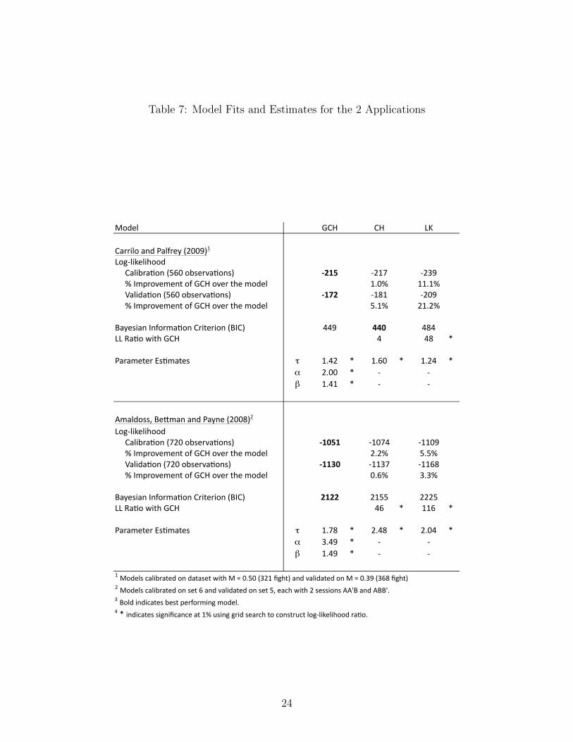
Table 7: Model Fits and Estimates for the 2 Applications

Model GCH CH   LK

Carrilo  and  Palfrey  (2009)1

Log-­‐likelihood          Calibra>on  (560  observa>ons) -­‐215 -­‐217 -­‐239          %  Improvement  of  GCH  over  the  model 1.0% 11.1%          Valida>on  (560  observa>ons) -­‐172 -­‐181 -­‐209          %  Improvement  of  GCH  over  the  model 5.1% 21.2%

Bayesian  Informa>on  Criterion  (BIC) 449 440 484LL  Ra>o  with  GCH 4 48 *

Parameter  Es>mates τ 1.42 * 1.60 * 1.24 *α 2.00 * -­‐ -­‐β 1.41 * -­‐ -­‐

Amaldoss,  BeUman  and  Payne  (2008)2

Log-­‐likelihood          Calibra>on  (720  observa>ons) -­‐1051 -­‐1074 -­‐1109          %  Improvement  of  GCH  over  the  model 2.2% 5.5%          Valida>on  (720  observa>ons) -­‐1130 -­‐1137 -­‐1168          %  Improvement  of  GCH  over  the  model 0.6% 3.3%

Bayesian  Informa>on  Criterion  (BIC) 2122 2155 2225LL  Ra>o  with  GCH 46 * 116 *

Parameter  Es>mates τ 1.78 * 2.48 * 2.04 *α 3.49 * -­‐ -­‐β 1.49 * -­‐ -­‐

1  Models  calibrated  on  dataset  with  M  =  0.50  (321  fight)  and  validated  on  M  =  0.39  (368  fight)2  Models  calibrated  on  set  6  and  validated  on  set  5,  each  with  2  sessions  AA'B  and  ABB'.3  Bold  indicates  best  performing  model.4  *  indicates  significance  at  1%  using  grid  search  to  construct  log-­‐likelihood  ra>o.

24

FIGURE 2

Fight Rate over Strength [0,1] with M = 718

0  

0.1  

0.2  

0.3  

0.4  

0.5  

0.6  

0.7  

0.8  

0.9  1  

Fight  Rate  

Strength  

Data  

GCH

 

LK  

25

FIGURE 3

Fight Rate over Strength [0,1] with M = 0.50

0  

0.1  

0.2  

0.3  

0.4  

0.5  

0.6  

0.7  

0.8  

0.9  1  

Fight  Rate  

Strength  

Data  

GCH

 

LK  

26

predicted fight rate of LK is almost always higher than the GCH model except in the higher

end of strength. This effect is generated by the model of opponents.

5.2 Coordination by Irrelevant Alternative

Amaldoss, Bettman and Payne (2008) demonstrated how coordination could be improved

by adding a weakly dominated alternative. In a 2x2 nonzero sum game, row player chooses

between A and B and column player chooses between L and R. There are two pure strategy

coordinating equilibria which pay better, (A, R) and (B, L). When a weakly dominated

(by one of the two original strategies) alternative was added to the choice set of the row

player, Amaldoss et al (2008) showed that the choice proportion of the dominating strategy

increased. Specifically, when A’ (weakly dominated by A) was added, the choice proportion

of A increased from 47.22% to 59.45%. Similarly, when B’ is added, the proportion of B

increased from 52.78% to 83.12% (see Table 5 of Amaldoss et al (2008)). Column players

chose R more frequently when A’ was added, increased from 51.81% to 72.92%. Hence, both

row and column players had higher proportion of coordination at (A, R), increased from an

average of 22.22% to 41.67%. Column players also chose L more frequently when B’ was

added, increased from 48.19% to 75.14%. This resulted in better coordination at (B, L),

increased from an average of 23.20% to 63.20% (see Table 7 of Amaldoss et al (2008)).

Similar to Amaldoss et al (2008), we analyze strategic thinking using the data generated

in their study 2, datasets 5 and 6. The two datasets use different payoff matrices. Each

dataset has two sessions, one with row strategies (A,B,A’) and another with (A,B,B’).9 Col-

umn players in both sessions have column strategies (L, R). We calibrate on dataset 6 and

validate on dataset 5.10 Bottom panel of Table 7 reports the parameters, the calibration and

9Minimum aversion picks up the asymmetric dominance in the (A,B,A’) sessions where A is favored by

level 0 row player but in the (A,B,B’) session, B is not favored by level 0 row player. In the (A,B,B’) session

the weakly dominant alternative B pays the minimum (same as B’) when column player picks R, hence no

strategy is favored by level 0 row player. In short, (A,B,B’) is a game with a specific form of asymmetric

dominance which GCH model does not cover.10Calibrating on dataset 5 yields a substantially better fit for GCH when compared to CH and LK where

log-likelihood for GCH is -1026 versus -1111 for CH and -1160 for LK. One reason that GCH fits better in

dataset 5 is due to the even higher contribution from capturing minimum aversion.

27

validation results.

GCH provides an improvement in log-likelihood of 23 points and 58 points over CH and LK

respectively. GCH also has a significant lead over the CH and the LK model in validation.

The parameter estimates of the GCH model are τ = 1.78, α = 3.49 and β = 1.49, compared

to τ = 2.48 for the CH model and τ = 2.04 for the LK model. The average thinking step

is about 2 when we look at the τ estimates from the 3 models. Stereotype bias seems to be

fairly strong at 3.49. When coupled with the τ estimates, it suggests that level 2 and above

respond mostly to level 1. Never worst strategies are 49% more favored by level 0.

To further understand the differences among the three models, we describes the predicted

behaviors of level k players using the (A,B,A’) session in dataset 6 (payoff matrix reproduced

in Table 8).

Table 8: (A,B,A’) session in Dataset 6 from Amaldoss et al [2008]

L R

A 16,16 20,24

A’ 8,22 20,12

B 24,20 8,8

Note: Payoffs in bold indicate the minimum payoff for

the corresponding columns or rows. The never worst

set for the row player consists of strategy A which

weakly dominates strategy A’. The never worst set

for column player is empty. There are two equilibria,

namely (A,R) and (B,L).

As indicated in Table 8, strategy A in the Never Worst set is preferred by level 0 row player

while level 0 column player randomizes between L and R. GCH predicts that the behavior

of row player level 3 and above stabilizes onto strategy A and the column player level 2 and

above stabilizes onto strategy R. Hence, GCH predicts the game to stabilizes onto (A, R),

one of the two equilibria, for players level 3 and above. While the CH model predicts that

row player level 5 and above chooses A and column player level 5 and above chooses R. In

other words, the GCH and CH models predict higher level players converging onto one of

28

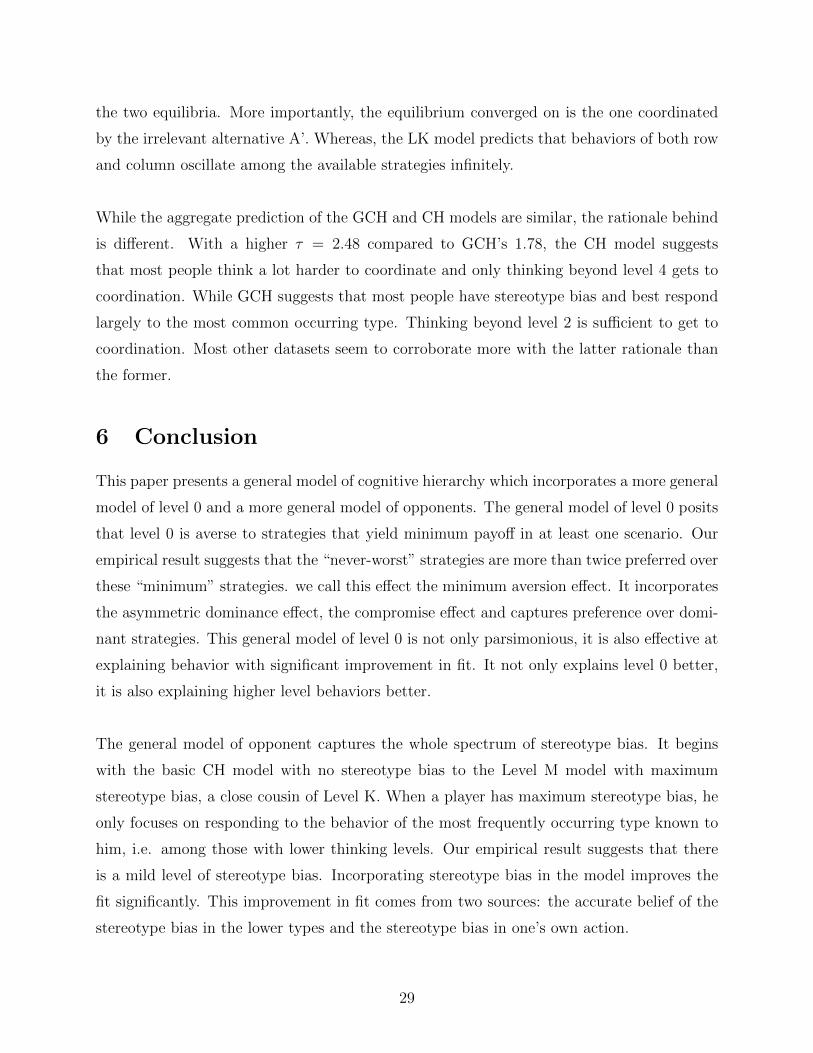
the two equilibria. More importantly, the equilibrium converged on is the one coordinated

by the irrelevant alternative A’. Whereas, the LK model predicts that behaviors of both row

and column oscillate among the available strategies infinitely.

While the aggregate prediction of the GCH and CH models are similar, the rationale behind

is different. With a higher τ = 2.48 compared to GCH’s 1.78, the CH model suggests

that most people think a lot harder to coordinate and only thinking beyond level 4 gets to

coordination. While GCH suggests that most people have stereotype bias and best respond

largely to the most common occurring type. Thinking beyond level 2 is sufficient to get to

coordination. Most other datasets seem to corroborate more with the latter rationale than

the former.

6 Conclusion

This paper presents a general model of cognitive hierarchy which incorporates a more general

model of level 0 and a more general model of opponents. The general model of level 0 posits

that level 0 is averse to strategies that yield minimum payoff in at least one scenario. Our

empirical result suggests that the “never-worst” strategies are more than twice preferred over

these “minimum” strategies. we call this effect the minimum aversion effect. It incorporates

the asymmetric dominance effect, the compromise effect and captures preference over domi-

nant strategies. This general model of level 0 is not only parsimonious, it is also effective at

explaining behavior with significant improvement in fit. It not only explains level 0 better,

it is also explaining higher level behaviors better.

The general model of opponent captures the whole spectrum of stereotype bias. It begins

with the basic CH model with no stereotype bias to the Level M model with maximum

stereotype bias, a close cousin of Level K. When a player has maximum stereotype bias, he

only focuses on responding to the behavior of the most frequently occurring type known to

him, i.e. among those with lower thinking levels. Our empirical result suggests that there

is a mild level of stereotype bias. Incorporating stereotype bias in the model improves the

fit significantly. This improvement in fit comes from two sources: the accurate belief of the

stereotype bias in the lower types and the stereotype bias in one’s own action.

29

With careful calibration and validation using the rich repertoire of datasets, the GCH model

provides a very robust and decent performance in one-shot games. More importantly, it pro-

vides an intuitive and viable explanation of the observed behaviors. We believe the model

has wider applicability. In the last section, we offers two application examples of this Gen-

eralized CH model.

For future research direction, we suggest that the GCH model can be applied with some

perturbations to other economic applications to provide a better understanding of the un-

derlying behaviors. In particular, our model of opponent can be parameterized to explain

how stereotype bias might vary depending on how subjects’ prior is primed; our model of

level 0 can be parameterized to capture the potential impact of game structure, and more

specifically the impact of payoff structure.

Appendix 1: Entry Game Analysis for the LM model

We have e(0, d) = 12

for all d, and

Ek(k − 1, d) =

e(k − 1, d) if k ≤ mode

e(mode, d) if k > mode

(10)

For k ≥ 1

e(k, d) =

{0 if Ek(k − 1, d) > d

1 if Ek(k − 1, d) < d(11)

We shall derive the condition on τ for the Poisson distribution when total entries is mono-

tonically increasing in demand. Given that the entry function of level k only depends on a

single lower level (whether it is k−1 or mode of the distribution), there is only one single cut-

point as d increases. For d < 12, level 1 will stays out, level 2 enters, and continuing with odd

30

level stay out and even levels enter, until the mode. If mode is even, then all levels above mode

stay out, otherwise, they enter. Hence, total entry is (1/2)f(0)+f(2)+f(4)+ · · ·+f(mode),

if mode is even; otherwise it is (1/2)f(0) + f(2) + f(4) + · · · + f(mode − 1) + f(mode +

1) + f(mode + 2) + · · · . For d > 12, level 1 enters since half of level 0 enter. Level 2 stays

out, and continuing with odd levels enter and even levels stay out until the mode. If mode

is even, then all levels above mode enter, otherwise, they stay out. Hence, total entry is

(1/2)f(0) + f(1) + f(3) + · · ·+ f(mode− 1) + f(mode+ 1) + f(mode+ 2) + · · · , if mode is

even; otherwise it is (1/2)f(0) + f(1) + f(3) + · · ·+ f(mode).

If mode is even, the condition of monotonically increasing entries requires total en-

tries in d < 1/2 to be less than total entries in d > 1/2. In other words, 1 − f(0) >

2(f(2) + f(4) + · · · + f(mode)), this is always true for the unimodal Poisson distribution

given the f(0) is exponentially decreasing in τ . If the mode is odd, we have the condition

that 1 − f(0) < 2(f(1) + f(3) + · · · + f(mode)), this condition is satisfied when τ ≤ 1.256.

Hence, total entries is monotonically increasing in demand when τ ≤ 1.256 in a Poisson

distribution of thinking levels.

References

Amaldoss, Wilfred, James R. Bettman and John W. Payne“Biased but Efficient:

An Investigation of Coordination Facilitated by Asymmetric Dominance,” Marketing

Science, 27(5), (2008), 903-921.

Binmore, Kenneth, Joe Swierzbinski and Chris Proulx, “Does Maximin Work?

An Experimental Study,” Economic Journal, 111, (2001), 445-464.

Bloomfield, Robert, “Learning a Mixed Strategy Equilibrium in the Laboratory,”

Journal of Economic Behavior and Organization, 25, (1994), 411-436.

Camerer, Colin F., Teck-Hua Ho and Juin-Kuan Chong, “A Cognitive Hierarchy

Theory of One-shot Games,” Quarterly Journal of Economics, 119(3), (2004), 861-898.

31

Carrillo, Juan D. and Thomas R. Palfrey, “The Compromise Game: Two-Sided

Adverse Selection in the Laboratory,” American Economic Journal: Microeconomics,

1(1), (2009), 151-181.

Cooper, David and John Van Huyck, “Evidence on the Equivalence of the Strategic

and Extensive Form Representation of Games,” Journal of Economic Theory, 110(2),

(2003), 290-308.

Costa-Gomes, Miguel and Vincent Crawford, ”Cognition and Behavior in Two-

Person Guessing Games: An Experimental Study,” American Economic Review, 96,

(2006), 1737-1768.

Costa-Gomes, Miguel, Vincent Crawford and Bruno Broseta, “Cognition and Be-

havior in Normal-form Games: An Experimental Study,” Econometrica, 69(5), (2001),

1193-1235.

Crawford, Vincent, “Boundedly Rational versus Optimization-Based Models of

Strategic Thinking and Learing in Games”, Journal of Economic Literature, 51, (2013),

512-527.

Crawford, Vincent and Nagore Iriberri, “Fatal Attraction: Salience, Naivete, and

Sophistication in Experimental Hide-and-Seek Games,” American Economic Review,

97(5), (2007), 1731-1750.

Goeree, Jacob, Charles Holt and Thomas Palfrey, “Risk Averse Behavior in Gener-

alized Matching Pennies Games,” Games and Economic Behavior, 45(1), (2003), 97-113.

Lieberman, Bernhardt, “Experimental studies of conflict in some two-person and

three-person games,” In J. H. Criswell, H. Solomon, and P. Suppes (Eds.), Mathemat-

ical Models in Small Group Processes. Stanford: Stanford University Press, (1962),

203-220.

Messick, David M., “Interdependent Decision Strategies in Zero-sum Games: A

32

Computer-controlled Study,” Behavioral Science, 12, (1967), 33-48.

Mookerjee, Dilip and Barry Sopher, “Learning and Decision Costs in Experi-

mental Constant-sum Games,” Games and Economic Behavior, 19, (1997), 97-132.

Nagel, Rosemarie, “Unraveling in Guessing Games: An Experimental Study,”

American Economic Review, 85(5), (1995), 1313-1326.

Ochs, Jack, “Games with Unique, Mixed Strategy Equilibria: An Experimental

Study,” Games and Economic Behavior, 10, (1995), 202-217.

O’Neill, Barry, “Nonmetric Test of the Minimax Theory of Two-person Zero-

sum Games,” Proceedings of the National Academy of Sciences, 84, (1987), 2106-2109.

Rapoport, Amnon and Amaldoss, Wilfred, “Mixed Strategies and Iterative Elim-

ination of Strongly Dominated Strategies: An Experimental Investigation of States of

Knowledge,” Journal of Economic Behavior and Organization, 42, (2000), 483-521.

Rapoport, Amnon and Boebel, Richard B., “Mixed Strategies in Strictly Com-

petitive Games: A Further Test of the Minimax Hypothesis,” Games and Economic

Behavior, 4, (1992), 261-283.

Stahl, Dale O., and Paul Wilson, ”Experimental Evidence on Players’ Models of

Other Players,” Journal of Economic Behavior and Organization, 25, (1994), 309-327.

Stahl, Dale O., and Paul Wilson, ”On Players Models of Other Players: Theory

and Experimental Evidence,” Games and Economic Behavior, 10, (1995), 218-254.

Tang, Fang-Fang, “Anticipatory Learning in Two-person Games: Some Experi-

mental Results,” Journal of Economic Behavior and Organization, 44, (2001), 221-32.

33