1

A Fuzzy Set-Based Approach to Range-Free Localization in

Wireless Sensor Networks1

Andrija S. Velimirović, Goran Lj. Djordjević, Maja M. Velimirović, Milica D. Jovanović

Faculty of Electronic Engineering, University of Nis, Aleksandra Medvedeva 14, P.O.

Box 73, 18000 Nis, Serbia

Abstract

Localization in Wireless Sensor Networks (WSNs) refers to the ability of determining the

positions of sensor nodes, with an acceptable accuracy, based on known positions of

several anchor nodes. Among the plethora of possible localization schemes, the Received

Signal Strength (RSS) based range-free localization techniques have attracted significant

research interest for their simplicity and low cost. However, these approaches suffer from

significant estimation errors due to low accuracy of RSS measurements influenced by

irregular radio propagation. In order to tackle the problem of RSS uncertainty, in this

work we propose a fuzzy set-based localization method as an enhancement of the ring-

overlapping scheme [12]. In the proposed method, first we use a fuzzy membership

function based on RSS measurements to generate fuzzy sets of rings that constrain sensor

node position with respect to each anchor. Then we generate fuzzy set of regions by

intersecting rings from different ring sets. Finally, we employ weighted centroid method

on the fuzzy set of regions to localize the node. The results obtained from simulations

demonstrate that our solution improve localization accuracy in the presence of radio

irregularity, but even for the case without radio irregularity.

Keywords: Wireless Sensor Networks, Range-free localization, Received Signal

Strength, Ring-overlapping, Fuzzy set theory.

1This work was supported by the Serbian Ministry of Science and Technological Development, project No. TR - 11020 - "Reconfigurable embedded systems".

2

1. Introduction

Recent advances in wireless communications, low-power design, and MEMS-based

sensor technology have enabled the development of relatively inexpensive and low power

wireless sensor nodes. The common vision is to create a large wireless sensor network

(WSN) through ad-hoc deployment of hundreds or thousands of such tiny devices able to

sense the environment, compute simple task and communicate with each other in order to

achieve some common objective, like environmental monitoring, target tracking,

detecting hazardous chemicals and forest fires, monitoring seismic activity, military

surveillance [1]. Most of these applications require the knowledge on the position of

every node in the WSN. However, in most cases, sensor nodes are deployed throughout

some region of interest without their position information known in advance. Thus, the

first task that has to be solved is to localize the nodes, i.e., to find out their spatial

coordinates in some fixed coordinate system. Determining the physical positions of

sensor nodes is a crucial problem in WSN operation because the position information is

used (i) to identify the location at which sensor readings originate, (ii) in energy aware

geographic routing, and (iii) to make easier network self-configuration and self-

organization. Also, in many applications the position itself is the information of interest

[2].

One possible way to localize sensor nodes is to use the commonly available Global

Positioning System (GPS), which offers 3-D localization based on direct line-of-sight

with at least four satellites [3]. However, attaching a GPS receiver to each sensor node is

highly impractical solution due to its high power consumption, high price, inaccessibility

(nodes may be deployed indoors, or GPS reception might be obstructed by climatic

conditions) and imprecision (the positioning error might be of 10-20m) [4]. A number of

localization systems and algorithms have been proposed recently specifically for WSNs,

which are generally classified into range-based and range-free localization schemes. The

range-based localization depends on the assumption that sensor nodes have the ability to

estimate the distance or angle to other nodes by means of one or more of the following

measurements: received signal strength (RSS), time of arrival (TOA), time difference of

3

arrival (TDOA), and angle of arrival (AOA) [5][6][7][8][9]. Although the range-based

schemes typically provide a lower estimation error than the range-free schemes, they

require installation of specific and expensive hardware (e.g., directive antennas) to obtain

relatively accurate distance (or angle) measurements and have weakness in the noisy

environments.

In contrast to range-based technique, the range-free scheme enables sensor nodes to

estimate their locations without relying on distance/angle measurements [2][4][10][11].

Such techniques generally require numerous anchors (location-aware nodes) which

enable location-unknown sensor nodes to determine their locations by exploiting the

radio connectivity information among nodes, or by comparing their RSS measurements

with those supplied by anchors or nearby nodes. Range-free solutions use only standard

features found in most radio modules as hardware means for localization, thus providing

more economic and simpler location estimates than the range-based ones. On the other

hand, the results of range-free methods are not as precise as those of the range-based

methods.

In this paper we propose a distributed range-free localization technique, called Fuzzy-

Ring, which utilizes the received signal strength information to estimate the relative

position of a sensor node with respect to a small number of randomly distributed anchors.

Similar to other area-based localization methods [11][12][13], Fuzzy-Ring uses beacons

broadcasted by anchors to isolate a region of the localization space where the sensor node

most probably resides. Like in ROCRSSI algorithm [12], the localization region is

defined as the intersection area of overlapping annular rings which constrain the position

of the sensor node with respect to each anchor. The rings are generated by comparison of

the signal strength a sensor node receives from a specific anchor and the signal strength

other anchors receive from the same anchor. The novelty of our localization scheme is to

represent overlapping rings as fuzzy sets with ambiguous boundaries. The use of the

fuzzy set theory is motivated by the fact that RSS measurements are usually inaccurate

due to a number of factors such as multipath propagation, reflection, interference and

shadowing among others. Such irregularity of the radio propagation creates non-circular

4

ring borders and might induce a significant localization error when a binary decision-

making model (“in-ring” versus “out-of-ring”) is employed, like in ROCRSSI. In our

approach, we use fuzzy membership functions based on the RSS information to represent

the degree to which a sensor node location is within different rings, which helps to

improve localization estimations, especially for sensor nodes located in proximity to ring

boundaries.

The rest of the paper is organized as follows: Section 2 introduces localization based on

comparison of RSS and discuses how fuzzy set theory can be applied in this range-free

approach. Section 3 presents the proposed localization approach. Results for the

simulations are shown in Section 4. Finally, Section 5 concludes this paper.

2. Localization based on comparison of RSS

RSS–based range–free algorithms only rely on the assumption that the RSS is a

decreasing function of the distance between transmitter and receiver. For example, if the

straight of the beacon signal that sensor node S receives from anchor A is smaller than

the straight of the same signal received by anchor B, then S can conclude that it is closer

to A then to B. A number of distance constraints, produced after a series of such

comparisons, will enable the sensor node to confine its position within a limited area of

the localization space.

Let consider a network with n=3 anchors placed at fixed known positions in 2-D

localization space shown in Fig. 1. Around each anchor the set of n-1 concentric circles is

placed. Radius of every circle equals distance between center anchor and one of n-1

remaining anchors. Each set of concentric circles partitions the localization space into n

rings numbered from 1 to n. The ring 1 corresponds to the area of the innermost circle,

while the ring n-1 corresponds to the outside area of the last circle. A localization region

is the intersection area of rings from different ring sets, while its area-code is the

sequence of the intersecting ring numbers, i.e. ring ranks. For example, shaded area in

Fig. 1 represents the region with area-code (2, 1, 2), i.e. the region which is obtained by

5

intersecting rings 2, 1 and 2 of anchors A1, A2, and A3, respectively. Note that for each

point p in this region, the area-code (2, 1, 2) defines the following set of distance-based

constraints:

d(A1, A2) ≤ d(A1, p) ≤ d(A1, A3)

d(A2, A2) ≤ d(A2, p) ≤ d(A2, A3)

d(A3, A2) ≤ d(A3, p) ≤ d(A3, A1)

where d(x, y) denotes the distance between two anchors/nodes.

Fig. 1. Rings, regions and area codes.

In an idealistic physical environment, RSS measured at a point further from an anchor is

always smaller then RSS measured at a point that is closer to the same anchor. As a

consequence, if we use RSS information for the regionalization of the localization space,

the resulting set of regions, i.e. the set of region area-codes, will be the same as one

obtained by using distance information. This means that a sensor node will always be

able to locate itself into the correct localization region by using the comparison of RSS

values, only. For example, the following set of RSS-based constraints will confine the

location of the sensor node S inside the region (2, 1, 2) of the network given in Fig. 1:

6

rss(A1, A2) ≥ rss(A1, S) ≥ rss(A1, A3)

rss(A2, A2) ≥ rss(A2, S) ≥ rss(A1, A3)

rss(A3, A2) ≥ rss(A3, S) ≥ rss(A1, A1)

where rss(x,y) denotes the strength of the signal broadcasted by anchor x as measured by

anchor/node y.

However, the radio propagation is usually not homogenous in all directions because of

the presence of multi-path fading and different path losses depending on the direction of

propagation. As a result, the ordering of the anchors based on comparison of RSS values

might not be identical with their ordering based on comparison of Euclidean distances,

which might induce localization errors. Let consider a partial distance-based regional

map of the network configuration with four anchors given in Fig. 2. A sensor node S,

depicted with square mark, is located in the region with area-code (3, 1, 1, 3). However,

due to inaccurate RSS measurements, S may easily came up with the wrong decision

regarding its regional area-code. For example, in order to correctly locate itself into ring 3

of the anchor A4, S should measure lower strength of the beacon signal broadcasted by A4

then anchor A3. However, because of the irregularity in radio propagation, there is a

chance for S to measure a higher RSS value then A3. Such an imprecision will cause the

sensor node S to choose the area-code (3, 1, 1, 2) instead of the correct one (3, 1, 1, 3). As

S is closer to the boundary of the A4’s ring 3 the chance for the wrong ring selection is

larger. Note that area code (3, 1, 1, 2) is valid, but wrong. Under some circumstances, S

may pick an area-code that does not even exist in distance-based regional map, i.e. it may

select so called invalid area-code. For example, an incorrect ring selection with respect to

anchor A2 could result in the area-code (3, 2, 1, 3). It is easy to see that this area-code

does not exist in the given regional map since 3rd rings of anchors A1 and A4 intersect in

two regions, only, i.e. in regions (3, 1, 1, 3) and (3, 4, 4, 3).

7

Fig. 2. A segment of distance-based regional map.

In ROCRSSI algorithm, the problem of incorrect ring/region selection is solved by

choosing the valid region (or regions) with the maximum number of intersecting rings.

However, in this approach, a small radio irregularity in the proximity of ring boundaries

may lead to the large localization error, as illustrated in Fig. 3(a). In order to overcame

the uncertainty of the RSS and the nonlinearity between the RSS and the distance, in this

work we suggest a different approach based of the fuzzy set theory. We use fuzzy sets to

model relationship between localization regions and the RSS information available to the

sensor node. When comparing its RSS measurements with those of anchors, the sensor

node will not select one region only, but it might choose two or more regions each with

different weight representing certainty of the decision. This concept is illustrated in Fig.

3(b). Different shades of gray indicate different weighs of the selected regions. Finally,

the center of gravity of the shaded area is used as the final location estimation.

(a) (b)

Fig. 3. ROCRSSI vs. fuzzy selection of localization regions.

A2

A3

S

8

3. Fuzzy-Ring Localization Algorithm

In this section, we describe our novel fuzzy set-based range-free localization scheme,

which we call Fuzzy-Ring. Fuzzy-Ring requires a heterogeneous wireless sensor network

composed of two sets of static nodes distributed across a planar sensing field: the set of

anchors, i.e. the nodes whose locations are known, and the set of sensor nodes, i.e. the

nodes whose locations are to be determined. For simplicity and ease of presentation we

limit the sensing field to 2-D, but with minor modifications our algorithm is capable of

operating in 3-D. Anchor nodes, or nodes with a prior knowledge of their locations in the

sensing field (obtained via GPS or other means such as pre-configuration), serve as

reference points, broadcasting beacon messages. They are assumed to be sparse and

randomly located. Both anchors and sensor nodes are equipped with omni-directional

antennas and RF transceivers with built-in RSS indicator (RSSI) circuitry. Anchors are

assumed to have a larger communication range than normal sensor nodes so that their

beacons can reach all wireless nodes in the network. The Fuzzy-Ring algorithm proceeds

in four phases: 1) Beacon exchange, 2) Distance-based regionalization, 3) RSS-based

regionalization, and 4) CoG calculation. These steps are performed at individual nodes in

a purely distributed fashion.

3.1. Beacon exchange

The Fuzzy-Ring algorithm requires every anchor to periodically send out beacon message

including its own ID. While receiving a beacon every anchor and sensor node samples

the received signal straight (RSS) and stores measured value together with the ID of the

transmitting anchor. At the end of this period, all anchors broadcast so-called localization

messages to all sensor nodes. Localization message includes anchor’s ID and its location

information, along with a vector containing the recorded RSS values of beacons it

received from other anchors. We assume that anchors are synchronized so that their

beacon and localization message transmissions do not overlap in time. Note that after

beacon exchange phase, each sensor node S knows not only locations of all anchors, but

9

also RSS values measured between each pair of anchors as well as between each anchor

and S, i.e.:

Vector [li], },...,1{ ni of anchors locations wherein li = (axi, ayi) is 2-D coordinate of

anchor Ai in the sensor field.

Vector [xi], },...,1{ ni of sensor node’s RSSI readings wherein xi is the strength of

the beacon signal that S received from anchor Ai.

Matrix [ri,j] of anchors’ RSSI readings wherein ri,j is the strength of the signal that

anchor Aj received form anchor Ai.

3.2. Distance-based regionalization

After collecting enough information, a sensor node can start the localization process. The

first step in this process is to create a distance-based regional map of the localization

space by using the known locations of all anchors. Let AS = {Ai}, i = 1... n, be the set of

anchors. Taking Ai as the center anchor, elements in AS can be arranged into the anchor

sequence Qi = (a0 = Ai, a1, ..., an-1, an = F) ordered by distance to Ai, wherein

}{\ ij AASa , }1,...,1{ nj , and F is a fictive anchor placed in infinity. Thus, d(Ai, aj)

≤ d(Ai, aj+1), },...,1{ nj . Each anchor sequence Qi, },...,1{ ni defines an ordered

sequences of distance-intervals Ti = ([0, d(Ai, a1)], ..., [d(Ai, aj), d(Ai, aj+1)], ..., [d(Ai, an-1),

∞]). For any point p in localization space and any anchor Ai, there is exactly one distance-

interval in Ti such that d(Ai, aj) ≤ d(Ai, p) ≤ d(Ai, aj+1). The rank of point p with respect to

anchor Ai, written as ranki(p), is the ordinal number of the corresponding distance-

interval in Ti. Area-code of point p, written as C(p), is defined as the sequence of its ranks

with respect to all anchors, i.e. c(p) = (rank1(p), ..., rankn(p)). Note that the order in which

the ranks are written in an area-code is determined by a predefined order of anchor IDs.

Localization region, R, with area-code C(R) = C is the set of all points in the localization

space with the same area-code, i.e. R = {p | c(p) = C}. Distance-based regional map,

denoted as D, is the set of area-codes of all regions identified in the localization space.

10

For the purpose of the proposed localization algorithm, each region is represented by the

following two attributes: (a) the area-code, and (b) the center of gravity (CoG). CoG of

region R is defined as the average location of all points in R. Since the analytical

procedure for finding regions and their CoGs is rather involved for resource constrained

sensor nodes due to the large number of floating point operations, we adopted an

approximate approach based on grid-scan algorithm [11][12]. In this algorithm, the

localization space is divided into uniform grid of M x M points, and the area-code is

determined at each point in the grid. Initially, the distance-based regional map, D, is

empty. In order to identify localization regions, the grid is scanned, point-by-point. For

each grid point p with coordinates (px, py) the area-code c(p) is first determined based on

its Euclidean distances to the anchors and pre-determined anchor sequences, and then the

regional map D is searched for that code. If the area-code c(p) is not found, it is inserted

into the map D, and the new region R is created with the code c(p). Four variables, C, X,

Y, and P, are associated with each region, representing its area-code, the sum of x-

coordinates, the sum of y-coordinates, and the total number of grid points in the region,

respectively. When the new region is created, its variables are initialized to C = C(p), P =

1, X = px, and Y = py. Otherwise, if D already contains the area-code C(p), variables X, Y,

and P of that region are updated; i.e. X = X + px, Y = Y + py and P = P + 1. After grid

scanning is completed, the region CoG coordinates are calculated as ),(P

Y

P

X.

3.3. RSS-based regionalization

In this algorithm step, sensor node creates a RSS-based regional map by comparing its

own RSSI readings with those gathered from anchors. Assume that RSS measurements

are in the range I = [0, RSS_max], and denote with ri,j the RSS value of the beacon signal

sent by anchor Ai as measured by jth anchor in anchor sequence Qi = (a0 = Ai, a1, ..., an-1,

an = F). We also assume that ri,0 = RSS_max, and ri,n = 0. The value of ri,j splits the RSS

range into two disjoint sub ranges: LTi,j = [0, ri,j], and GTi,j = [ri,j, RSS_max]. Note that

LTi,0 = GTi,n = I. The RSS-interval with rank j in respect to anchor Ai, denoted as RIi,j,

represents the sub range of RSS values between those measured by two successive

11

anchors, ai,j and ai,j+1, in anchor sequence Qi. In the case of monotonic attenuation of

radio signal, i.e. when ri,j ≥ ri,j+1, RSS-interval is defined as RIi,j = [ri,j, ri,j+1]. However,

due to the irregular radio propagation, the monotonic characteristic might not be always

satisfied, and it might happen that ri,j ≤ ri,j+1, i.e. RIi,j = [ri,j+1, ri,j]. Thus, the RSS-interval

can be defined as:

,, ∩ , , ,

, ∩ , , , (1)

Fig. 4 shows the relationship between distance-intervals and RSS-intervals along one

particular anchor sequence. RSS values of A1’s beacon signal as measured by three

different sensors, S1, S2, and S3 are denoted with rs1, rs2, and rs3, respectively. Note that

in 2-D localization space each distance-interval corresponds to one ring centered in

anchor A1. Note also that due to the anomaly in the radio propagation, anchor A2

measures a larger RSS value than A3 introducing overlapping of RSS-intervals. Using the

“rigid” comparison of RSS values both sensors S1 and S2 will be localized within the ring

A1 – A4 since 1,121, RIrsrs . Although we may have a high degree of confidence in this

decision as sensor S1 is concerned, the real location of sensor S2 is much more uncertain

due to its proximity to the boundary between RSS intervals RI1,1 and RI1,2. The radio

irregularity makes the position of sensor node S3 even more uncertain since its RSS

measurement, rs3, fits in three RSS intervals, RI1,2, RI1,3 and RI1,4.

Fig. 4. Relationship between RSS-intervals and distance-intervals.

12

In order to minimize the effect of the uncertainty in RSS values on transition from RSS-

based to distance-based domain, we explicitly incorporate the uncertainty in the modeling

of RSS intervals using the concepts of fuzzy set theory. First, we represent RSS sub

ranges, , and  , , as fuzzy sets , ,,

∈  and  ,

,,

∈ , where  , , and , represent membership functions defined

as:

,

1 , 1

1

2 ,1

1

2 , 1 , 1

0 , 1

,1

,

A graphical interpretation of membership functions  , , and , is given in Fig. 5.

Parameter P, which we call the level of fuzzification, is involved to enable adaptation to

various levels of radio propagation irregularity. The value of ∈ 0,1 controls the width

of fuzzy region of the membership functions. Functions   , , and , are used by

a sensor node when it compares the straight of the beacon signal it received from anchor

Ai, x, with the RSS value , of the same beacon measured by jth anchor in the anchor

sequence headed in Ai. When x is outside the fuzzy region, the outcome of this

comparison is strictly “greater then” or “less then” describing the full membership in one

of two RSS sub-ranges, LTi,j or GTi,j. On the other hand, when x is in the fuzzy region, the

result of the comparison is a partial membership in both RSS sub-ranges.

Fig. 5. Membership functions.

)(, xjiLT )(, xji

GT

13

Fuzzy set , ,,

∈ representing RSS-interval RIi,j is derived according

to (1) by applying the fuzzy intersection operation on fuzzy sets , and  , . For

membership function    , we use:

  ,   

,  

,1 , ,

  ,

  ,

1 , ,

(2)

Note that expression (2) is known in fuzzy set theory as bounded product (or bold

intersection) [14]. A sensor node uses function   , to determine the degree of its

membership in jth ring placed around anchor Ai.

Given vector X = (x1, x2, ..., xn) of sensor node’s RSS measurements, the fuzzy-ring set

with respect to anchor Ai, written as , is the set of ranks of all RSS-intervals with non-

zero degree of membership in respect to anchor Ai, i.e.,

,   ,

|  ,

0 , 1, … ,

Note that elements of  are integers in range [1, n]. Note also that ⊆ P({1, 2, ..., n}),

where P denotes a power set. Cardinality of a fuzzy-ring set depends on several factors,

such as the number of anchors, the value of parameter P, and the level of radio

propagation irregularity.

The RSS-based regional map is Cartesian product of fuzzy-ring sets:

… , ,

where , , … ,  is area-code, and ,∙

,∙ … ∙

,.

14

Elements of are region area-codes. The degree of membership of an area-code in

RSS-based regional map is derived by multiplying degrees of sensor node membership in

all rings that intersect in the corresponding region.

The last operation of the fuzzification process filters out all invalid area-codes from the

RSS-based regional map. The output is the fuzzy set of area-codes, , that contains all

area-codes of that also belong to the distance-based regional map, D, i.e.

∩ , | ∈ , ∈

Note that degrees of membership of area-codes in are the same as in  . In some

rare cases it may happen that does not contain any area-code. In such situations, there

are two options: to left the sensor node unknown (i.e. not-localized), or to repeat the

fuzzification process with a larger value of parameter P. We implement the second one.

3.4. CoG Calculation

Given the fuzzy set of area-codes,  , the goal of the final step of the localization

process is to find the crisp real value that represent the estimated location of the sensor

node. Note that two numeric attributes are associated with each area-code in  : (a) the

CoG of the corresponding localization region, and (b) the degree of membership in  .

We use Center of Area method (CoA) to produce final location estimation:

_∑ ∙∈

∑ ∈

,∑ ∙∈

∑ ∈

where  and  are x- and y-coordinate of CoG of the region with area-code

C.

15

4. Simulation Results

We implement Fuzzy-Ring localization algorithm in a custom WSN simulator build in

C++, and conducted several experiments to evaluate its performances. In addition, we

compare our results to the ROCRSSI algorithm. Our evaluation is based on the

simulation of a benchmark set of 60 different network configurations categorized into six

subsets of ten networks with the same number of anchors. We analyze network

configurations with 3 to 8 anchors. All networks in one subset are created by varying

positions of n anchors within the same basic setup of 200 sensor nodes randomly

deployed in a circular area of 100 m in diameter. In our simulations, we intend to

illustrate the impact of the number of anchors, the degree radio propagation irregularity,

and the level of fuzzification on the localization error. The performance of two

localization methods is evaluated using the location estimation error defined as

(d/D)*100%, where d is the Euclidian distance between the real location of a sensor node

and its estimated location, and D is the diameter of the localization area.

Radio propagation model

We adopt the Degree Of Irregularity (DOI) radio propagation model introduced in [11]

and subsequently extended in [12]. In this model, the signal strength is defined as

2/)( dKC , where C is a constant, d is the distance between the receiver and the

transmitter, and K() is the coefficient representing the difference in path loss in different

directions. K() is calculated according to (3) where ]360,0[ o , rand is a random

number uniformly distributed in range [-1,1], s , and t [12]. The parameter

DOI is used to denote the irregularity of the radio pattern. It is defined as the maximum

signal straight variation per unit degree change in the direction of radio propagation.

When DOI value is 0, there is no variation in the signal straight which results in a

perfectly circular radio model. When DOI > 0, large DOI values represent large variation

of radio irregularity. Examples of two characteristic DOI values of this irregular radio

pattern model are shown in Fig. 6.

16

 

 1 01       (3)

Fig. 6. Irregular radio patterns for different values of DOI.

Localization Error when varying P

In order to analyze the impact of the fuzzification level, expressed by the value of

parameter P, on the localization error we simulate Fuzzy-Ring algorithm under various

degrees of radio propagation irregularity in a network with NA=5 anchors. The value of

parameter P defines the width of the boundary region of fuzzy membership functions.

When P value is 0, the fuzzification is practically switched-off by forcing selection of

one ring per anchor, only. When P is greater than 0, the chance of selecting multiple rings

per anchor increases. In this way, the value of P directly influences the cardinality of the

fuzzy set of regions. Fig. 7 shows the location error as a function of P for four

characteristic values of DOI.

DOI=0.05 DOI=0.2

17

Fig. 7. Localization error vs. level of fuzzification (P) for four different degrees of radio

propagation irregularity (DOI).

As can be seen from Fig. 7, the fuzzy approach is beneficial even in the regular (i.e.

circular) radio propagation scenario (i.e. when DOI value is 0). The regular radio

propagation pattern guaranties an ideal “1-1” matching between regions in distance- and

RSS-based regional maps enabling the Fuzzy-Ring algorithm to always select the correct

localization region, even without fuzzification (P=0). The only source of localization

errors is due to the distance between the CoG of the region and the real location of the

sensor node. When P > 0, the result of fuzzification process is the fuzzy set of regions

that includes multiple localization regions with different weights. This can move the CoG

toward the real location of the sensor node. On the other hand, an irregular radio

propagation pattern (DOI > 0) creates non-circular region borders causing a non-ideal

mapping between distance- and RSS-based localization regions. Without the fuzzification

(P=0), localization error is influenced not only by the inter-region errors but also by the

wrong ring selection. On the other hand, with the fuzzification switched-on (P>0) the

fuzzy set of region will likely include the correct region along with several nearby

regions which will partially compensate the inaccuracy of RSS measurements.

As can be seen from Fig. 7, for every value of DOI there is an optimal value of the

parameter P, Popt, for which the Fuzzy-Ring algorithm achieves the best performances.

For analyzed range of DOI values, the Popt ranges from 0.25, for DOI=0, to 0.65, for DOI

NA=5

0

2

4

6

8

10

0 0.1 0.2 0.3 0.4 0.5 0.6 0.7P

Avr

. Lo

cat

ion

Err

or

[% a

rea

dia

m.]

DOI=0

DOI=0.05DOI=0.1

DOI=0.2

18

= 0.2. Based on the above results, we suggest that the value of P should be set to 0.3 –

0.4 in order to achieve the minimal additional localization error caused by non-optimal

selection of P. For example, by using P=0.35, independently of DOI, the maximal

additional localization error is less than 10% in respect to Popt over the analyzed range of

DOI.

Localization Error when varying number of anchors

In this experiment, we study the influence of the number of anchors, NA, on localization

error. We apply both ROCRSSI and Fuzzy-Ring algorithms to all network configurations

in the benchmark set with ∈ 0, 0.05,0.1,0.2 and P set to 0.35. Fig. 8 shows the

location errors as a function of the number of anchors deployed. Each data point in these

graphs represents the average value of 20.000 localization trials. First, for every NA we

simulate 10 different anchor configurations within the network of 200 sensor nodes.

Second, for each anchor configuration, 10 runs with different random seeds for DOI were

executed.

From Fig. 8, we can observe that Fuzzy-Ring always outperforms ROCRSSI in terms of

localization error, no matter whether the radio propagation is regular or irregular. For

example, Fig. 8(b) shows that when we set the number of anchors at 6, Fuzzy-Ring

achieves 0.04D accuracy, which is 28% more accurate than the ROCRSSI. Thus, Fuzzy-

Ring algorithm enables us to deploy a smaller number of anchors to obtain the same level

of performances as with ROCRSSI. For example, when DOI is 0.05, the Fuzzy-Ring only

needs 5 anchors to achieve the same localization error as ROCRSSI with 8 anchors.

However, it is important to note that Fuzzy-Ring is more computationally intensive then

ROCRSSI. Based on the above results, we suggest that the optimal number of anchors

should be 5 or 6 because deploying a larger number of anchors results in marginal

improvement of localization accuracy, only.

19

(a) (b)

(c) (d)

Fig. 8. Localization error vs. number of anchors for: (a) DOI = 0; (b) DOI = 0.05; (c) DOI =

0.1; (d) DOI = 0.2.

Localization Error when varying DOI

In this experiment, the results of which are shown Fig. 9, we quantify the degree of

localization performance degradation in the presence of radio irregularity. We conduct

the analysis on the network configuration with 5 anchors under various degrees of radio

propagation irregularity (DOI). For Fuzzy-Ring algorithm we set the level of

fuzzification to P=0.35. From Fig. 9, we observe that with the increase of DOI values, the

DOI = 0

0

2

4

6

8

10

12

14

3 4 5 6 7 8

NA

Avr

. Lo

catio

n E

rro

r [%

are

a d

iam

.]

ROCRSSI

Fuzzy Ring

DOI = 0.05

0

2

4

6

8

10

12

14

3 4 5 6 7 8

NA

Avr

. Lo

cat

ion

Err

or

[% a

rea

dia

m.]

ROCRSSI

Fuzzy Ring

DOI = 0.1

0

2

4

6

8

10

12

14

16

3 4 5 6 7 8

NA

Av

r. L

oca

tion

Err

or

[% a

rea

dia

m.]

ROCRSSI

Fuzzy Ring

DOI = 0.2

0

2

4

6

8

10

12

14

16

18

20

3 4 5 6 7 8

NA

Avr

. Lo

cat

ion

Err

or

[% a

rea

dia

m.]

ROCRSSI

Fuzzy Ring

20

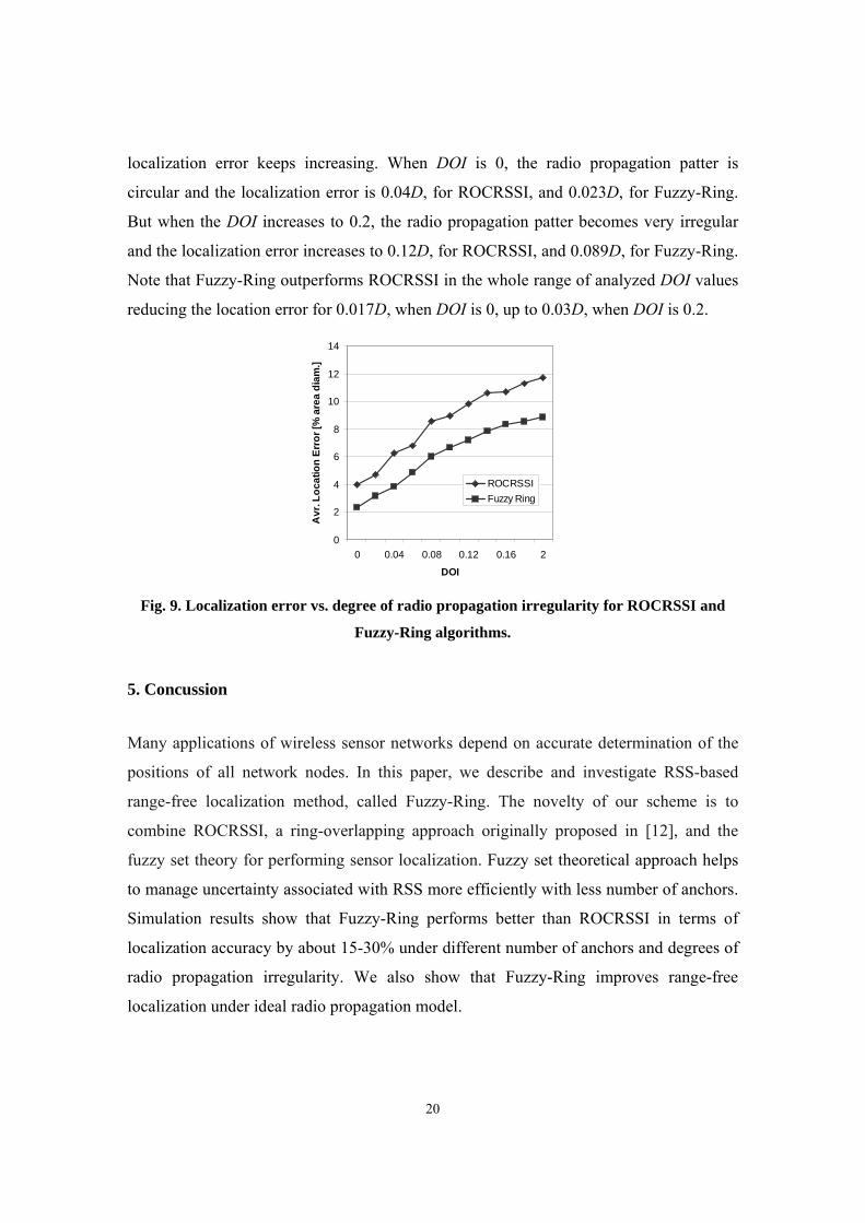
localization error keeps increasing. When DOI is 0, the radio propagation patter is

circular and the localization error is 0.04D, for ROCRSSI, and 0.023D, for Fuzzy-Ring.

But when the DOI increases to 0.2, the radio propagation patter becomes very irregular

and the localization error increases to 0.12D, for ROCRSSI, and 0.089D, for Fuzzy-Ring.

Note that Fuzzy-Ring outperforms ROCRSSI in the whole range of analyzed DOI values

reducing the location error for 0.017D, when DOI is 0, up to 0.03D, when DOI is 0.2.

Fig. 9. Localization error vs. degree of radio propagation irregularity for ROCRSSI and

Fuzzy-Ring algorithms.

5. Concussion

Many applications of wireless sensor networks depend on accurate determination of the

positions of all network nodes. In this paper, we describe and investigate RSS-based

range-free localization method, called Fuzzy-Ring. The novelty of our scheme is to

combine ROCRSSI, a ring-overlapping approach originally proposed in [12], and the

fuzzy set theory for performing sensor localization. Fuzzy set theoretical approach helps

to manage uncertainty associated with RSS more efficiently with less number of anchors.

Simulation results show that Fuzzy-Ring performs better than ROCRSSI in terms of

localization accuracy by about 15-30% under different number of anchors and degrees of

radio propagation irregularity. We also show that Fuzzy-Ring improves range-free

localization under ideal radio propagation model.

0

2

4

6

8

10

12

14

0 0.04 0.08 0.12 0.16 2

DOI

Av

r. L

oca

tion

Err

or

[% a

rea

dia

m.]

ROCRSSI

Fuzzy Ring

21

This paper does not consider the way to adapt the level of fuzzification to the varying

degree of radio propagation irregularity. This remains for a future work. In our future

work, we would also like to test the proposed scheme under more network scenarios such

as limited radio range of anchors, and to study the effect of topology of anchor nodes on

localization error.

6. References

[1] F. Akyildiz, W. Su, Y. Sankarasubramaniam, and E. Cayirci, ”Wireless sensor networks: A

survey”, Computer Networks, vol. 38, no. 3, pp. 393–422, 2002.

[2] N. Bulusu, J. Heidemann, and D. Estrin, “GPS-less low-cost outdoor localization for very

small devices”, IEEE Personal Communications, vol. 7, no. 5, pp. 28 -34, Oct. 2000.

[3] B. H. Wellenhoff, H. Lichtenegger, and J. Collins, Global positions system: theory and

practice, Fourth Edition, Springer Verlag, 1997.

[4] D. Nicolescu, B. Nath, “DV based positioning in ad hoc networks”, Journal of

Telecommunication Systems, vol. 22, no. 1, pp. 267–280, 2003.

[5] G. Mao, B. Fidan, and B. Anderson, “Wireless Sensor Networks Localization Techniques”,

Computer Networks, vol. 51, no. 10, pp. 2529-2553, 2007.

[6] D. Niculescu, B. Nath, “Ad hoc positioning system (APS) using AOA”, In Proc. of the 22nd

Annual Joint Conference of the IEEE Computer and Communications Societies, San

Francisco, USA, pp. 1734−1743, 2003.

[7] Y. Kwon, K. Mechitov, S. Sundresh, W. Kim, and G. Agha, “Resilient Localization for

Sensor Networks in Outdoor Environments”, In Proc. of 25th IEEE International Conference

on Distributed Computing Systems (ICDCS), pp. 643-652, 2005.

[8] A. Savvides, C. C. Han, and M. B. Srivastava, “Dynamic fine-grained localization in ad-hoc

networks of sensors”, In Proc. of the seventh annual international conference on Mobile

computing and networking (MobiCom 2001), pp. 166–179, 2001.

[9] P. Bahl, and V. N. Padmanabhan, “RADAR: An in-building RF-based user location and

tracking system”, INFOCOM 2000. Nineteenth Annual Joint Conference of the IEEE

Computer and Communications Societies, Proc. of IEEE, vol. 2, pp. 775-784, March 2000.

22

[10] R. Stoleru, T. He, J. A. Stankovic “Range-free Localization,” chapter in Secure

Localization and Time Synchronization for Wireless Sensor and Ad Hoc Networks, editors: R.

Poovendran, C. Wang, and S. Roy, Advances in Information Security series, vol. 30,

Springer, 2007.

[11] T. He, C. Huang, B.M. Blum, J. A. Stankovic, and T. Abdelzaher, “Range-Free

Localization Schemes for Large Scale Sensor Networks”, In Proc. of the ninth annual

international conference on Mobile computing and networking (MobiCom 2003), San Diego,

California, pp. 81-95, September 2003.

[12] C. Liu, T. Scott, K. Wu, and D. Hoffman, “Range-Free Sensor Localization with Ring

Overlapping Based on Comparison of Received Signal Strength Indicator”, International

Journal of Sensor Networks (IJSNet), vol. 2, no. 5, pp. 399-413, 2007.

[13] V. Vivekanandan, V. W. S. Wong, “Concentric Anchor-Beacons (CAB)

Localization for Wireless Sensor Networks”, IEEE International Conference on

Communications, ICC’06, Istanbul, 2006, vol. 9, pp. 3972-3977.

[14] D. J. Dubois, H. Prade, Fuzzy Sets and Systems: Theory and Applications, Academic

Press, 1980.