a fully non-linear model for three-dimensional overturning ...guyenne/publications/ijnmf01.pdf · a...
TRANSCRIPT

INTERNATIONAL JOURNAL FOR NUMERICAL METHODS IN FLUIDSInt. J. Numer. Meth. Fluids 2001; 35: 829–867
A fully non-linear model for three-dimensionaloverturning waves over an arbitrary bottom
Stephan T. Grillia,*,1, Philippe Guyenneb,2 and Frederic Diasc,3
a Ocean Engineering Department, Uni6ersity of Rhode Island, Narragansett, RI, U.S.A.b Institut Non-Lineaire de Nice, UMR 6618 CNRS-UNSA, Valbonne, France
c Ecole Normale Superieure, CMLA, UMR8536 CNRS, Cachan Cedex, France
SUMMARY
An accurate three-dimensional numerical model, applicable to strongly non-linear waves, is proposed.The model solves fully non-linear potential flow equations with a free surface using a higher-orderthree-dimensional boundary element method (BEM) and a mixed Eulerian–Lagrangian time updating,based on second-order explicit Taylor series expansions with adaptive time steps. The model is applicableto non-linear wave transformations from deep to shallow water over complex bottom topography up tooverturning and breaking. Arbitrary waves can be generated in the model, and reflective or absorbingboundary conditions specified on lateral boundaries. In the BEM, boundary geometry and field variablesare represented by 16-node cubic ‘sliding’ quadrilateral elements, providing local inter-element continuityof the first and second derivatives. Accurate and efficient numerical integrations are developed for theseelements. Discretized boundary conditions at intersections (corner/edges) between the free surface or thebottom and lateral boundaries are well-posed in all cases of mixed boundary conditions. Higher-ordertangential derivatives, required for the time updating, are calculated in a local curvilinear co-ordinatesystem, using 25-node ‘sliding’ fourth-order quadrilateral elements. Very high accuracy is achieved in themodel for mass and energy conservation. No smoothing of the solution is required, but regridding to ahigher resolution can be specified at any time over selected areas of the free surface. Applications arepresented for the propagation of numerically exact solitary waves. Model properties of accuracy andconvergence with a refined spatio-temporal discretization are assessed by propagating such a wave overconstant depth. The shoaling of solitary waves up to overturning is then calculated over a 1:15 planeslope, and results show good agreement with a two-dimensional solution proposed earlier. Finally,three-dimensional overturning waves are generated over a 1:15 sloping bottom having a ridge in themiddle, thus focusing wave energy. The node regridding method is used to refine the discretizationaround the overturning wave. Convergence of the solution with grid size is also verified for this case.Copyright © 2001 John Wiley & Sons, Ltd.
KEY WORDS: boundary element method; breaking ocean waves; non-linear surface waves; numericalwave tank; potential flow; three-dimensional flows
* Correspondence to: Ocean Engineering Department, University of Rhode Island, Narragansett, RI 02882, U.S.A.Fax: +1 401 8746837.1 E-mail: [email protected] E-mail: [email protected] E-mail: [email protected]
Recei6ed July 1999Copyright © 2001 John Wiley & Sons, Ltd. Re6ised June 2000

S. T. GRILLI, P. GUYENNE, AND F. DIAS830
1. INTRODUCTION
Over the past two decades, the development of increasingly accurate and efficient numericalmodels of highly non-linear surface waves has been a continuous challenge in the ocean andcoastal engineering and science communities. Indeed, wave dynamics govern most physicalprocesses occurring (e.g., air–sea interactions, wave shoaling and breaking, wave-inducedcoastal currents, surf-zone dynamics, . . . ), and engineering design methods used (e.g., forbreaking wave impact pressures on coastal and off-shore structures, . . . ) in these areas.
When dealing with waves prior to breaking, the most successful methods, whether theoreti-cal or numerical, have been based on potential flow theory, which neglects both viscous androtational effects on the wave flow. The governing equation in this case—the continuityequation—is a Laplace’s equation for the potential. This linear partial differential equation(PDE) can efficiently be solved in a boundary integral equation (BIE) formulation, using eithera free space or a more specialized Green’s function; or by eigenfunction or polynomialexpansions. Non-linear terms are included in the dynamic and kinematic free surface boundaryconditions for the potential, and methods usually differ in accuracy, range of applicability, andnumerical efficiency by the way they deal with these terms.
A traditional approach in most wave theories and numerical models based on these has beento define so-called small parameters (e.g., wave steepness, ratio of water depth to wave-length, . . . ) and to express truncated series expansions of free surface boundary conditions andgeometry as a function of these parameters (see, e.g., Mei [1]). In this line, wave propagationmodels based on so-called extended higher-order Boussinesq equations have recently producedquite impressive results in coastal areas, for shallow and intermediate waters (e.g., Wei et al.[2]).
When dealing with strongly non-linear waves close to breaking or starting to break (i.e.,overturning waves), methods based on small parameters and, in most cases, on a single-valuedEulerian description of the free surface, become irrelevant. For such cases, governing equationsmust be solved in their primitive form and the time integration must be based on a mixedEulerian–Lagrangian (MEL) formulation following fluid particle trajectories on the freesurface. Many such numerical solutions of potential flow theory (referred to as ‘fullynon-linear potential flow’ (FNPF) problems) have been developed, mostly in two dimensions(2D), and have been shown to model the physics of wave overturning in deep and intermediatewater (e.g., Dommermuth et al. [3] and Skyner [4]) and wave shoaling and breaking over slopes(e.g., Grilli et al. [5,6], Li and Raichlen [7]), with a surprising degree of accuracy. Let usmention for completion that recent improvements in computer power have also led to anincreasing use of modernized volume of fluid (VOF) methods solving complete Navier–Stokesequations for free surface flows (e.g., Grilli [8], Guignard et al. [9]; Chen et al. [10]). SuchVOF methods can model post-breaking waves, but they are computationally expensive,particularly in three dimensions (3D), and suffer from numerical diffusion leading to artificialloss of wave energy over long distances of propagation. Hence, in such cases, unless thepost-breaking wave flow is the focus of the study, FNPF theory, which is more accurate andefficient, is preferred over VOF methods. A promising recent development is the coupling of
Copyright © 2001 John Wiley & Sons, Ltd. Int. J. Numer. Meth. Fluids 2001; 35: 829–867
3D OVERTURNING WAVES OVER AN ARBITRARY BOTTOM 831
FNPF and VOF methods for pre- and post-breaking wave flows respectively (Guignard et al.[11]).
Thus, most studies to date dealing with transformations of waves leading to breaking havebeen based on an FNPF formulation. Furthermore, in most FNPF models, Laplace’s equationhas been solved with a higher-order boundary element method (BEM; Brebbia [12]), eitherbased on Green’s identity or on Cauchy integral theorem formulations. Time integration offree surface boundary conditions (expressed in an MEL formulation) has been performedeither using a time marching (Runge–Kutta) or a predictor–corrector (Adams–Bashforth–Moulton) scheme, or both (e.g., Longuet-Higgins and Cokelet [13]), or a Taylor seriesexpansion method (Dold and Peregrine [14]). Early computations following this approach weretwo-dimensional and restricted to space–periodic waves over constant depth [13–16], but morerecent two-dimensional models can accommodate both arbitrary incident waves and complexbottom topographies (e.g., Klopman [17], Grilli et al. [18], Cointe [19], Cooker [20], andOhyama and Nadaoka [21]). Most recent models also directly work in a physical space region,i.e., in a numerical wa6e tank (NWT), in which incident waves are generated at one extremityand reflected, absorbed, or radiated at the other extremity (see Grilli and Subramanya [22] andGrilli and Horrillo [23] for details).
Three-dimensionality, in addition to producing quite formidable numerical problems, posesmore difficult geometric and far-field representation problems than two-dimensionality. Innaval hydrodynamics and offshore engineering fields many authors have proposed (mostlyBEM based but often with constant panels) three-dimensional models for weakly and, morerecently, fully non-linear permanent or transient wave patterns created by submerged sources,or submerged/floating bodies moving at constant or variable speed (e.g., Dommermuth andYue [24], Forbes [25], Boo [26], and Lee et al. [27]), or transient wave diffraction, run-up, andforces on surface piercing cylinders (e.g., Isaacson [28], Yang and Ertekin [29], Cheung et al.[30], Lalli et al. [31], Celebi et al. [32], and Ferrant [33]). In these problems, the free surface isalways single-valued and, by assuming infinite or constant depth (image method) and openocean, the problem often reduces to only discretizing the free surface and the body.
Only a few attempts have been reported of solving FNPF problems for transient non-linearwave propagation in general 3D-NWTs, two of them modeling overturning waves. Romate[34] developed a three-dimensional (constant) panel method, which he applied to weaklynon-linear waves generated by a wavemaker and propagating in a narrow 3D-NWT. His timestepping method was similar to that in Reference [13] but results were quite limited andaffected by spurious waves, maybe due to problems at intersections between the free surfaceand lateral boundaries. Xu and Yue [35,36] calculated three-dimensional overturning waves ina doubly-periodic computational domain with infinite depth (i.e., only the free surface wasdiscretized). They used a higher-order BEM based on Green’s identity, with a doubly periodicGreen’s function in the x- and y-directions, quadratic isoparametric boundary elements, andan MEL time stepping similar to that of Reference [13]. As in the two-dimensional solution ofReference [13], sawtooth instabilities eventually developed near wave crests; these wereeliminated by smoothing, typically applied every few time steps. As in Reference [13], initiallytwo-dimensional periodic waves were made to break by specifying an asymmetric surfacepressure. Broeze [37] developed a method similar to Xu and Yue’s and was able to produce the
Copyright © 2001 John Wiley & Sons, Ltd. Int. J. Numer. Meth. Fluids 2001; 35: 829–867
S. T. GRILLI, P. GUYENNE, AND F. DIAS832
initial stages of overturning waves over a bottom obstacle; numerical instabilities were alsoexperienced, which limited computations. Boo et al. [38] produced irregular non-linear wavesin a 3D-NWT; they used a higher-order BEM and a semi-Lagrangian time marching schemesimilar to that in Reference [13]. Sawtooth instabilities occurred and were eliminated bysmoothing. Ferrant [33,39] developed a 3D-NWT based on a BEM with linear elements, andan MEL time stepping similar to that of Reference [13]. He studied wave radiation–diffractionby floating bodies and wave forces on surface piercing cylinders; an annular absorbing beachwas used at the exterior boundary. Note that, in the previous two studies, BEM matrices weremaintained constant for several time steps in order to save on computational time. Celebi etal. [32] studied diffraction of periodic waves around bottom mounted columns, using a BEMwith an MEL time stepping, in an NWT having both wave generation and absorbing beachboundaries.
Reviews of two- and three-dimensional highly non-linear wave problems to date can befound in Romate [34], Yeung [40], Peregrine [41], Grilli [42], Grilli and Subramanya [43], Tsaiand Yue [44], and Kim et al. [45].
From the above it appears that FNPF theory can be used to model overturning waves overan arbitrary bottom. Many such two-dimensional and a few three-dimensional solutions (i.e.,NWTs) have been proposed. Among these, the most stable and accurate models were those inwhich higher-order spatial and temporal discretizations methods were used, and importantproblems such as corner/edge boundary conditions and numerical integrations were carefullyaddressed. Importantly, in the few existing higher-order two-dimensional models [14,18,22],strongly non-linear waves were accurately propagated over long distances and/or time, up tooverturning, without the need for smoothing or filtering of the solution. The non-linear natureof the problem and lack of dissipation in FNPF theory indeed are such that numerical errors,even very small, remain an integral part of the solution and build up as a function of timethrough superposition and non-linear interactions. Therefore, such errors must be minimizedby seeking optimum accuracy in all numerical aspects of the model.
In the present study, the experience gained by the authors in developing accurate and stablenumerical methods for 2D-FNPF-NWTs is applied to the development of a new, similarlyaccurate, 3D-FNPF-NWT for strongly non-linear waves. The model is developed using ahigher-order 3D-BEM and an MEL time updating, based on a second-order Taylor seriesexpansion, with adaptive time steps, similar to that used in the two-dimensional model ofReference [18]. The model is applicable to non-linear wave transformations up to overturningand breaking, from deep to shallow water over arbitrary bottom topography. Arbitrary wavescan be generated in the NWT by wavemakers or directly on the free surface (note only thelatter method will be detailed here). Reflective and absorbing boundary conditions areimplemented on lateral boundaries of the NWT; for the latter in a way similar to Grilli andHorrillo [23] (note no application of absorbing boundaries will be presented here). Geometryand field variables are represented on the NWT boundary by 16-node cubic ‘sliding’ two-dimensional elements similar, in principle, to the one-dimensional 4-node ‘middle-interval-interpolation (MII)’ elements introduced by Grilli and Subramanya [22] in their two-dimensional model. Such elements provide local inter-element continuity of the first andsecond derivatives. Accurate and efficient numerical integrations are developed for theseelements. Discretized boundary conditions at intersections (corner/edges) between the free
Copyright © 2001 John Wiley & Sons, Ltd. Int. J. Numer. Meth. Fluids 2001; 35: 829–867
3D OVERTURNING WAVES OVER AN ARBITRARY BOTTOM 833
surface or the bottom and lateral boundaries are well-posed in all cases of mixed boundaryconditions following the methods introduced by Grilli and Subramanya [22] and Grilli andSvendsen [46]. Higher-order tangential derivatives required for the time updating are calculatedin a local curvilinear co-ordinate system using two-dimensional 25-node sliding fourth-orderelements similar in principle to the 5-node one-dimensional elements introduced by Grilli andSvendsen [46] for calculating s-derivatives in their two-dimensional model. Node regridding toa higher resolution can be specified over selected areas of the free surface. Details of the modeldevelopment and implementation are given in Section 2 and applications are presented inSection 3. These are first aimed at assessing the model properties of accuracy and convergencewith a refined spatio-temporal discretization, by checking errors on conservation of mass andenergy for solitary wave propagation over constant depth. The shoaling of solitary waves upto breaking is then calculated over a 1:15 plane slope in a quasi-two-dimensional configurationand results are compared with two-dimensional results by Grilli et al. [6]. Finally, three-dimensional overturning waves are calculated over a 1:15 sloping bottom having a ridge in themiddle, thus focusing wave energy. The node regridding method is tested in the latterapplication and convergence of results with grid size is verified.
2. THE MATHEMATICAL AND NUMERICAL MODEL
2.1. Go6erning equations and boundary conditions
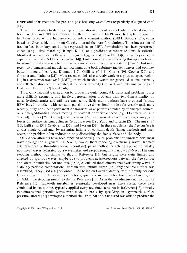
Equations for fully non-linear potential flows with a free surface are listed in the following.The velocity potential f(x, t) is used to represent inviscid irrotational three-dimensional flowsin Cartesian co-ordinates (x, y, z), with z the vertical upward direction (and z=0 at theundisturbed free surface). The velocity is defined by (Figure 1)
Figure 1. Sketch of computational domain for 3D-BEM solution of FNPF equations. The domain isdefined for x]x0. Note a region of constant depth h=h0 is specified for x5x0+d0, beyond whichdepth is set to h=b(x, y). Tangential vectors at point R(t) of the free surface Gf(t) are defined as (s, m)
and outward normal vector as n.
Copyright © 2001 John Wiley & Sons, Ltd. Int. J. Numer. Meth. Fluids 2001; 35: 829–867
S. T. GRILLI, P. GUYENNE, AND F. DIAS834
u=9f= (u, 6, w) (1)
The continuity equation in the fluid domain V(t), with boundary G(t), is a Laplace equationfor the potential
92f=0, in V(t) (2)
The corresponding three-dimensional free space Green’s function is defined as (e.g., Brebbia[12])
G(x, xl)=1
4pr, with
(G(n
(x, xl)= −1
4p
r ·nr3 (3)
and
r=x−xl (4)
with r= �r � being the distance from point x (x, y, z) to the reference point xl (xl, yl, zl),both being on boundary G, and n representing the outward normal unit vector to the boundaryat point x.
Green’s second identity transforms Equation (2) into the BIE
a(xl)f(xl)=&
G(x)
!(f(n
(x)G(x, xl)−f(x)(G(n
(x, xl)"
dG (5)
in which a(xl)=ul/(4p), with ul the exterior solid angle made by the boundary at point xl (i.e.,2p for a smooth boundary; Brebbia [12]).
Boundary G is divided into various parts with different boundary conditions (Figure 1). Onthe free surface Gf(t), f satisfies the non-linear kinematic and dynamic boundary conditions
DRDt
=u=9f on Gf(t) (6)
Df
Dt= −gz+
12
9f ·9f−pa
ron Gf(t) (7)
respectively, with R the position vector of a free surface fluid particle, g the acceleration dueto gravity, pa the atmospheric pressure, r the fluid density, and the material derivative beingdefined as
DDt (
(t+u ·9 (8)
Copyright © 2001 John Wiley & Sons, Ltd. Int. J. Numer. Meth. Fluids 2001; 35: 829–867
3D OVERTURNING WAVES OVER AN ARBITRARY BOTTOM 835
Various methods can be used for wave generation in the model (Grilli et al. [23,46]). Forinstance, when waves are generated by simulating a wavemaker motion on the ‘open sea’boundary of the computational domain, Gr1(t), motion and velocity [xp, up ] are specified overthe wavemaker as
x=xp and(f
(n=up ·n on Gr1(t) (9)
where overlines denote specified values.Along the bottom Gb and other stationary parts of the boundary, referred to as Gr2, a
no-flow condition is prescribed as
(f
(n=0, on Gb and Gr2 (10)
Note G Gf@Gr1@Gr2@Gb.
2.2. Time integration
Free surface boundary conditions (6) and (7) are integrated at time t to establish both the newposition and the boundary conditions on the free surface Gf(t) at a subsequent time (t+Dt)(with Dt a varying time step).
Following the method implemented in Grilli et al.’s [18,22] two-dimensional model, second-order explicit Taylor series expansions are used to express both the new position R(t+Dt) andthe potential f(R(t+Dt)) on the free surface, in an Eulerian–Lagrangian formulation
R( (t+Dt)=R(t)+DtDRDt
(t)+(Dt)2
2D2RDt2 (t)+O[(Dt)3] (11)
f( (R(t+Dt))=f(t)+DtDf
Dt(t)+
(Dt)2
2D2f
Dt2 (t)+O[(Dt)3] (12)
Coefficients in these Taylor series are expressed as functions of the potential, its partial timederivative, and the normal and tangential derivatives of both of these along the free surface(details of calculations of tangential derivatives are given in a following section).
More specifically, first-order coefficients are given by Equations (6) and (7), which requirescalculating (f, (f/(n) on the free surface. This is done by solving the BIE (5) at time t, withboundary conditions (9), (10), and (12) (see next section). Second-order coefficients areobtained from the material derivative of Equations (6) and (7), which requires also calculating((f/(t, (2f/(t (n) at time t ; this is done by solving a BIE similar to Equation (5) for thesefields. The free surface boundary condition for this second BIE is obtained from the Bernoulliequation (7) after solution of the first BIE for f as
Copyright © 2001 John Wiley & Sons, Ltd. Int. J. Numer. Meth. Fluids 2001; 35: 829–867
S. T. GRILLI, P. GUYENNE, AND F. DIAS836
(f
(t= −gz−
12
9f ·9f−pa
r, on Gf(t) (13)
For a wave generation by a wavemaker, Equation (9) gives
(2f
(t (n=((up ·n)(t
, on Gr1(t) (14)
and for the bottom and other stationary boundaries
(2f
(t (n=0 on Gb and Gr2 (15)
Note that the BIEs for f and (f/(t are solved at time t and thus both correspond to thesame boundary geometry and have the same discretized form (see next section). Therefore, thesolution of the second BIE only takes a small fraction of the time (typically a few per cent)needed for the solution of the first BIE (when using a direct method of solution). This makesthis time stepping method very efficient, particularly when compared with higher-orderRunge–Kutta or Adams–Bashforth–Moulton schemes used in other studies (e.g., Longuet-Higgins and Cokelet [13], Romate [34]) which often require multiple evaluations of the BIE (5)for several intermediate times per time step. Other advantages of this time stepping scheme areof being explicit and using spatial derivatives of the field variables along the free surface in thecalculation of values at (t+Dt). This provides more stability to the computed solution andmakes it possible to use larger time steps with a similar accuracy, thus making the overallsolution more efficient.
2.3. Boundary discretization
2.3.1. Classical BEM. The BIE (5) for f, and its equivalent for (f/(t, are solved by a BEM[12].
In this method, the boundary is discretized into NG collocation nodes and MG higher-orderelements are used to define local interpolations in between m of these nodes. Thus, within thekth such element, Ge
k, both the boundary geometry and field variables (denoted by u=f andq=(f/(n for simplicity and generality) are discretized using shape functions. Here, shapefunctions are analytically defined, as higher-order polynomials, over a single reference elementGj,h, to which the MG ‘Cartesian’ elements of arbitrary shape are transformed by a change ofvariable. The intrinsic co-ordinates on the reference element are denoted by (j, h)� [−1, 1].Variations of the geometry and field variables over each element k are described by their nodalvalues, x j
k, ujk, and qj
k, and by the local shape functions Nj(j, h) as
x(j, h)=Nj(j, h)x jk (16)
u(j, h)=Nj(j, h)ujk and q(j, h)=Nj(j, h)qj
k (17)
Copyright © 2001 John Wiley & Sons, Ltd. Int. J. Numer. Meth. Fluids 2001; 35: 829–867

3D OVERTURNING WAVES OVER AN ARBITRARY BOTTOM 837
where j=1, . . . , m locally numbers the nodes within each element Gek, for k=1, . . . , MG, and
the summation convention is applied to repeated subscripts.The shape functions are selected as polynomials of (j, h), whose coefficients are found by
requiring that u(j, h) take the value uik at node x i
k, i.e., in Equation (17)
u(j(x ik), h(x i
k))=Nj(ji, hi)ujk=ui
k
Hence, for the ith node of an m-node reference element, shape functions must satisfy
Nj(ji, hi)=dij with i, j=1, . . . , m on Gj,h (18)
and dij is the Kronecker symbol. Values of (ji, hi) only depend on the element shape (i.e.,triangular, quadrilateral) and degree (i.e., linear, quadratic). The solution of Equation (18) forselected element shape and degree thus provides corresponding closed form expressions for theshape functions (see next section). Note when the same shape functions are used for both thegeometry and the field variables, one defines so-called isoparametric elements.
2.3.2. The 3D-MII method. Isoparametric elements can provide a high-order approximationwithin their area of definition but only offer C0 continuity of the geometry and field variablesat the common nodes in between elements.
Based on the experience acquired in two-dimensional problems, for such highly non-linearwater wave problems one needs to define elements that are both higher-order within their areaof definition and at least locally C2 continuous in between elements. To do so, variousmethods, including cubic-spline-based elements, were used in two-dimensional models [22,46].Here, elements are defined using an extension of the so-called MII method introduced by Grilliand Subramanya [22] in their two-dimensional model. Boundary elements are 4-node quadri-laterals with cubic shape functions defined using both these and additional neighboring nodesin each direction, for a total of m=16 nodes. Hence, only part of the interval of variation(usually the middle part) of the cubic shape functions is used for calculating the boundaryintegrals in Equation (5) (Figure 2).
Figure 2. Sketch of 16-node cubic 3D-MII Cartesian element Gek and corresponding reference element
Gj,h. Quadrilateral element nodes are indicated by symbols (), and additional nodes by symbols (�).The curvilinear co-ordinate system (s, m, n) has been marked at point r of the element. (j0, h0) marks the
bottom left node of the quadrilateral, transformed as part of the reference element by Jk.
Copyright © 2001 John Wiley & Sons, Ltd. Int. J. Numer. Meth. Fluids 2001; 35: 829–867

S. T. GRILLI, P. GUYENNE, AND F. DIAS838
In the present 3D-MII method, two-dimensional bi-cubic shape functions are defined on thereference element as the product of two one-dimensional cubic shape functions N %c(m), withc=1, . . . , 4 and m� [−1, 1], i.e.
Nj(j, h)=N %b( j)(m(j, j0))N %d( j)(m(h, h0)) (19)
with b and d=1, . . . , 4; j=4(d−1)+b, and property (18) implying
N %c(mi)=dic with mi=2i−5
3(20)
for i=1, . . . , 4. Hence, solving Equation (20)
N %1(m)=116
(1−m)(9m2−1), N %2(m)=916
(1−m2)(1−3m),
N %3(m)=916
(1−m2)(1+3m), N %4(m)=116
(1+m)(9m2−1) (21)
For the MII method, the additional transformation from m to the intrinsic coordinates (j, h)on the reference element is formally expressed as
m(x, x0)=x0+13
(1+x) (22)
with x=j or h and x0=j0 or h0= −1, −1/3, or 1/3, depending on which of the ninequadrilaterals defined by the m=16 nodes is selected (Figure 2). Note this selection dependson the location of the element with respect to the intersections between various parts of theboundary (such as the free surface and lateral boundaries).
2.3.3. Discretized BIEs. Integrals in Equation (5) are transformed into a sum of integrals overthe boundary elements, each of which is calculated within the reference element Gj,h. To do so,the curvilinear change of variables introduced above [x� (j, h)] is expressed for element Ge
k bya Jacobian matrix Jk obtained as follows. Two orthogonal tangential vectors are defined atpoint x(j, h) of the boundary as (using Equations (17) and (18))
(x(j
=(Nj(j, h)(j
x jk=
!(N %b( j)(m(j, j0))(m
(m
(jN %d( j)(m(h, h0))
"x j
k,
(x(h
=(Nj(j, h)(h
x jk=
!N %b( j)(m(j, j0))
(N %d( j)(m(h, h0))(m
(m
(h
"x j
k (23)
with j=1, . . . , m on Gek (k=1, . . . , MG) and from Equation (22)
Copyright © 2001 John Wiley & Sons, Ltd. Int. J. Numer. Meth. Fluids 2001; 35: 829–867
3D OVERTURNING WAVES OVER AN ARBITRARY BOTTOM 839
(m
(j=(m
(h=
13
Corresponding tangential unit vectors are further defined as
s(j, h)=1h1
(x(j
and m(j, h)=1h2
(x(h
(24)
with the scale factors
h1=)(x(j
)and h2=
)(x(h
)(25)
A third vector is defined at the same point in the normal direction, as
(x(z
=(x(j
×(x(h
(26)
The corresponding unit normal vector is thus defined as
n(j, h)=1
h1h2
(x(z
=s×m with)(x(z
)=h1h2 (27)
This vector will be pointing in the outward direction with respect to the domain if directions(s, m) of the considered element are such that their cross product is outward oriented (this isonly a matter of definition of the element nodes numbering).
The Jacobian matrix is defined as
Jk=!(x(j
,(x(h
, n"T
and the determinant of the Jacobian matrix to be used in boundary integrals of Equation (5)for the kth element, by definition of an elementary surface element and with Equations (25)and (27), is given by
�Jk(j, h)�=h1h2 for k=1, . . . , MG on G (28)
which can be analytically calculated at any point of the element Gek, by using Equations
(23)–(25), with Equation (21).After transformation, the following discretized forms are obtained for the integrals in
Equation (5):
Copyright © 2001 John Wiley & Sons, Ltd. Int. J. Numer. Meth. Fluids 2001; 35: 829–867

S. T. GRILLI, P. GUYENNE, AND F. DIAS840
&G(x)
(f
(nGl dG= %
NG
j=1
! %MG
k=1
&Gj,h
Nj(j, h)G(x(j, h), xl)�Jk(j, h)� dj dh" (f(n
(xj)
= %NG
j=1
! %MG
k=1
Dljk" (fj
(n= %
NG
j=1
Kljd (fj
(n(29)
&G(x)
f(Gl
(ndG= %
NG
j=1
! %MG
k=1
&Gj,h
Nj(j, h)(G(x(j, h), xl)
(n)
Jk(j, h)� dj dh"
f(xj)
= %NG
j=1
! %MG
k=1
Eljk"fj= %
NG
j=1
Kljnfj (30)
in which l=1, . . . , NG and Dk and Kd denote so-called local (i.e., for element k) and global(i.e., assembled) Dirichlet matrices, and Ek and Kn are Neumann matrices. Note j is nowexpressed in the global node numbering on the boundary and denotes nodal values for elementk. Expressions for the Green’s function, the shape functions, and the Jacobian to be used inEquations (29) and (30) are given by Equations (3), (19), (21), and (28) respectively.
Using Equations (29) and (30), the discretized form of the BIE (5) finally reads
alul= %NG
j=1
{Kljd qj−Klj
n uj} (31)
in which l=1, . . . , NG.Boundary conditions are introduced in Equation (31); these are: (i) Dirichlet conditions for
u=f or (f/(t (Equations (12) or (13)); and (ii) Neumann conditions for q=(f/(n or(2f/(t (n (e.g., Equations (9), (10) or (14), (15)). The final algebraic system is assembled bymoving nodal unknowns to the left-hand side and keeping specified terms on the right-handside
{Cpl+Kpln }up−Kgl
d qg=Kpld qp−{Cgl+Kgl
n }ug (32)
where l=1, . . . , NG; g=1, . . . , Ng refers to nodes with Dirichlet condition on boundary Gf
and p=1, . . . , Np refers to nodes with Neumann condition on boundary Gr1@Gr2@Gb. C is adiagonal matrix made of coefficients al.
2.3.4. Solution of the algebraic system of equations. The solution of the algebraic system ofequations (32) initially implemented in the 3D-NWT was based on Kaletsky’s direct lower–upper (LU) elimination method, for which the CPU time is proportional to the cube of thenumber of nodes in the discretization. This method was used in some of the applicationspresented hereafter, which have small or moderate grid sizes, and were run on a Mac G3-266MHz powerbook or a G4-450 MHz computer. As we will see, for such small cases, theassembling of the system matrix through numerical integration, which is proportional to thenumber of elements (i.e., nodes), is more time consuming than the solution of the system itself.
The last applications presented in this paper, however, have much larger grid sizes and wererun on a CRAY-C90 supercomputer. For such cases, the solution of the system matrix takesan increasingly large part of the total CPU time, and it is desirable to use a (faster) iterative
Copyright © 2001 John Wiley & Sons, Ltd. Int. J. Numer. Meth. Fluids 2001; 35: 829–867

3D OVERTURNING WAVES OVER AN ARBITRARY BOTTOM 841
method to solve Equations (32). The ‘generalized minimal residual’ (GMRES) algorithm, alsoused by Xu and Yue [35,36], was implemented in the 3D-NWT, with preconditioning by the‘symmetric successive overrelaxation’ (SSOR) method (relaxation parameter equal to 0.6), withan initial solution equal to that of the earlier time step. The downside, however, is that for thetype of time stepping scheme used here, two full systems of equations must be solved at eachtime step—one for f and one for (f/(t—with an iterative method, whereas with a directmethod the solution of the second system takes only a few per cent of the time needed to solvethe first system. Nevertheless, results showed that for large systems of say more than 2000nodes and a similar accuracy, the GMRES-SSOR method is faster when used in the 3D-NWTthan the direct solution.
2.3.5. Rigid mode method. Coefficients Cll in Equation (32) can be obtained through a direct,purely geometric, calculation of solid angles ul at nodes of the discretized boundary. Thesecoefficients, however, can be indirectly obtained through a more accurate and efficientapproach, referred to as ‘rigid mode’ method by analogy with structural analysis problems(Brebbia [12]).
By considering a homogeneous Dirichlet problem, where a uniform field u=cst"0 isspecified over the whole boundary G (thus NG=Ng), one can show that normal gradients qmust vanish at each node. Thus, Equation (32) simplifies to
{Cjl+Kjln}uj=0 (33)
which requires that the summation in curly brackets vanishes for all l. Thus, by isolating thediagonal terms in the left-hand side, we get
{Cll+Klln}= − %
NG
j(" l)=1
Kjln, l=1, . . . , NG (34)
which specifies the value of the diagonal term of a row of Equation (33) as minus the sum ofits off-diagonal coefficients. These diagonal terms are directly substituted in the discretizedsystem (32).
This method was shown to significantly improve the conditioning of algebraic systems suchas Equation (32), and thus the accuracy of their numerical solution [18] (particularly foriterative methods). Physically, for potential flows this also corresponds to specifying that thediscretized problem exactly satisfies a zero global flux condition in a specific case.
2.3.6. Discretized boundary conditions at corners. Boundary conditions and normal directionsare in general different on intersecting parts of the boundary, such as between the free surfaceor the bottom, and the lateral boundary of the computational domain (Figure 1). Suchintersections are referred to as edges, and corresponding discretization nodes as corners. To beable to specify such differences in the model corners are represented by double-nodes for whichco-ordinates are identical but normal vectors are different [18,46]. Thus, two differentdiscretized BIEs (Equation (32)) are expressed for each node of a corner double-node.
For Dirichlet–Neumann boundary conditions we have, for instance, equations (i) for l=pon the wavemaker boundary Gr1; and (ii) for l= f on the free surface Gf. Since the potential
Copyright © 2001 John Wiley & Sons, Ltd. Int. J. Numer. Meth. Fluids 2001; 35: 829–867

S. T. GRILLI, P. GUYENNE, AND F. DIAS842
must be unique at a given location, however, one of these two BIEs must be modified in thefinal discretized system, to explicitly satisfy fp=ff (i.e., ‘continuity of the potential’), wherethe overline indicates that the potential is specified on the free surface. For Neumann–Neumann boundary conditions at corners we have, for instance, equations (i) for l=p on thewavemaker boundary Gr1; and (ii) for l=b on the bottom Gb. The potential continuityequation for this case reads fp−fb=0, both of these being unknown. Similar continuityrelationships are expressed for (f/(t at corners, in the corresponding BIE.
Note at the intersection between three boundaries, triple-nodes are specified for which threeBIE equations are expressed, two of which are replaced in the final algebraic system byequations specifying continuity of the potential (and of (f/(t).
2.3.7. Grid generation. A simple and efficient method is implemented in the model forgenerating discretizations in the 3D-NWT with a minimum number of parameters. Referringto Figure 1, the grid for a typical problem is generated by specifying the geometricalparameters: x0, d0, depth h0, the length l0 in the x-direction and width w0 in the y-direction,and the varying depth b(x, y); the latter being also automatically calculated for a simplesloping bottom or a ridge. Discretization parameters Mx, My, and Mz are also given, whichrepresent the number of MII quadrilateral elements in each direction. Note because of the waytangential derivatives are calculated (see below), there must be at least four elements in eachdirection.
2.4. Numerical integrations
Due to their complex analytical form, integrals in Equations (29) and (30) are numericallycalculated for each collocation point xl. For each element k these integrals are represented bylocal matrices Dlj
k and Eljk.
When the collocation node l does not belong to the integrated quadrilateral element (i.e.,l" j(k)=1, . . . , 4), a standard Gauss–Legendre quadrature method is used. When node ldoes belong to the element (i.e., Figure 3, j= l) distance r in Green’s function and its normalgradient becomes zero at one of the nodes of the element (Equations (3) and (4)). It can beshown [12] that when j= l, integrals Dlj
k are weakly singular (thus integrable with finiteL2-norm), whereas integrals Elj
k are non-singular. For the former integrals, special methods of‘singularity extraction’ are detailed below. For the latter integrals, in fact, the strong singular-ity occurring when r�0 was already removed, to become part of coefficients al, and it can beshown that the remaining part is proportional to the boundary curvature at xl. In any case,when the ‘rigid mode method’ is used, terms such as Ell
k are indirectly calculated in their globalform Kll
n by Equation (34).Finally, due to the form of Green’s function (3), non-singular integrals may still have a
highly varying kernel when distance r becomes small, albeit non-zero, in the neighborhood ofa collocation point. Such situations may occur near intersections of boundary parts (e.g., suchas between the free surface and lateral boundaries) or in other regions of the free surface, suchas overturning breaker jets, where nodes are close to elements on different parts of theboundary. In such cases, a standard Gauss quadrature, with a fixed number of integrationpoints, may fail to accurately calculate such integrals. One thus talks of ‘almost’ or ‘quasi-singular’ integrals. Grilli and Subramanya [47], for instance, showed for two-dimensional
Copyright © 2001 John Wiley & Sons, Ltd. Int. J. Numer. Meth. Fluids 2001; 35: 829–867

3D OVERTURNING WAVES OVER AN ARBITRARY BOTTOM 843
Figure 3. Sketch of co-ordinate transformations for weakly singular integrals in a quadrilateral elementGj,h, part of the 16-node cubic MII reference element (Figure 2). Axes (j %, h %) can be located at points
l=1, . . . , 4. The case of collocation node l=2 is given as an example.
problems that the loss of accuracy of Gauss integrations (with ten integration points) for suchquasi-singular integrals may be several orders of magnitudes, when the distance to thecollocation node becomes very small. For such two-dimensional cases, Grilli and Svendsen [46]developed an adaptive integration scheme based on a binary subdivision of the referenceelement and obtained almost arbitrary accuracy for the quasi-singular integrals when increas-ing the number of subdivisions. This method, however, can be computationally expensive andGrilli and Subramanya [47] developed a more efficient method that essentially redistributesintegration points around the location of the quasi-singularity (point of minimum distancefrom an element k to the nearest collocation node xl). A method similar to Grilli andSvendsen’s but applicable to three-dimensional problems is implemented in this study, anddetailed below.
2.4.1. Regular integrals. For 3D-MII elements, regular integrals in Equations (29) and (30) arecalculated with a bi-directional Gauss–Legendre quadrature method, with NL points in eachdirection. These integrals take the form
I ljk=
& +1
−1
& +1
−1
Fljk(j, h) dj dh= %
NL
g=1
%NL
h=1
wgwhFljk(lg, lh) (35)
where Fljk represents either one of the kernels in integrals Dlj
k or Eljk, and (wi, wj) and (lg, lh)
are Gauss weights and points respectively.For more efficiency in the numerical model, once NL is selected values of one-dimensional
shape functions N %c(m(x, x0)) and their derivatives with respect to m are precalculated for x=li
(i=1, . . . , NL), c=1, . . . , 4, and x0= −1, −1/3, and 1/3. From these, the two-dimensionalshape functions Nj and their partial derivatives are calculated with Equations (19) and (23).
Copyright © 2001 John Wiley & Sons, Ltd. Int. J. Numer. Meth. Fluids 2001; 35: 829–867
S. T. GRILLI, P. GUYENNE, AND F. DIAS844
2.4.2. Weakly singular integrals. Weakly singular integrals correspond to terms Dljk in Equation
(29) for j= l. In this case, the singular kernel of the integrals is first modified in order to geta form to which a polar co-ordinate transformation removing the weak 1/r singularity can beapplied. This is followed by further changes of variable and a final Gauss–Legendre numericalquadrature (Badmus et al. [48]). We have
Dljk=
&Gj,h
f jk(j, h)G(x(j, h), xl) dj dh with f j
k(j, h)=Nj(j, h)�Jk(j, h)� (36)
that is
Dljk=
14p
& +1
−1
& +1
−1
1r(x(j, h), xl)
f jk(j, h) dj dh (37)
where the singularity is located at node xl of the discretization, corresponding to co-ordinates(jl, hl) on the reference element.
A new co-ordinate system, centered on node (jl, hl), is defined within the reference elementas
j %=j−jl and h %=h−hl (38)
and Equation (37) becomes
Dljk=
14p
&& 1r %
Fjk(j %, h %) dj % dh % (39)
with
r %=j %2+h %2 and Fjk(j %, h %)=
r %r(x(j(j %), h(h %)), xl)
f jk(j(j %), h(h %)) (40)
where the function Fjk is non-singular (as could be seen by taking its limit for r�0) and the
integration limits for j % and h % depend on the position of the singularity.Polar co-ordinates (r %, 8) centered on (jl, hl) are then introduced (Figure 3) such that
j %=r % cos!
8+ (l−1)p
2"
and h %=r % sin!
8+ (l−1)p
2"
(41)
with l=1, . . . , 4. Noting that dj % dh %=r % dr % d8 and accounting for the geometry of thereference element, Equation (39) becomes
Dljk=
14p
!& p/4
0
d8& 2/cos 8
0
Fjk(r %, 8) dr %+
& p/2
p/4
d8& 2/sin 8
0
Fjk(r %, 8) dr %
"(42)
Copyright © 2001 John Wiley & Sons, Ltd. Int. J. Numer. Meth. Fluids 2001; 35: 829–867

3D OVERTURNING WAVES OVER AN ARBITRARY BOTTOM 845
where Equations (38) and (41) are used to relate (r %, 8) to (j, h) in Fjk. Limits of integrations
in Equation (42) are transformed into [−1, +1] by a last change of variable to (r¦, 8 %) andwe get
Dljk=
164
& +1
−1
d8 %!
r %12m
& +1
−1
Fjk(r %12, 812) dr¦+r %23
m& +1
−1
Fjk(r %23, 823) dr¦
"(43)
which can be integrated by a bi-directional Gauss–Legendre quadrature method as
Dljk=
164
%NL
i=1
%NL
j=1
wiwj{r %12m Fj
k(r %12, 812)+r %23m Fj
k(r %23, 823)} (44)
where (wi, wj) are Gauss weights, with
812=p
8(1+li) and 823=
p
8(3+li) (45)
r %12m =
2cos 812 and r %23
m =2
sin 812 (46)
and
r %12=r %12
m
2(1+lj) and r %23=
r %23m
2(1+lj) (47)
where (li, lj)� [−1, +1] are Gauss points.Again, for more efficiency, once NL is selected in the numerical model, values of 812, 823,
r %12m , r %23
m , r %12, and r %23 are precalculated for (li, lj) values, from which (j ij12,23, h ij
12,23) values areobtained using Equations (38) and (41) for l=1, . . . , 4. Then, one-dimensional shape func-tions N %c(m(x, x0)) and their derivatives with respect to m, to be used in Equations (19) and (23),are precalculated for x=j ij
12,23 or h ij12,23 (i, j=1, . . . , NL); c, l=1, . . . , 4; and x0= −1, −1/3,
and 1/3. From these, the two-dimensional shape functions Nj and their partial derivatives arecalculated using Equations (19) and (23).
2.4.3. Quasi-singular integrals. To identify possible quasi-singular integrals in the discretizeddomain, both distance and intercept angle thresholds are checked for each collocation nodel=1, . . . , NG and each quadrilateral boundary element k=1, . . . , MG.
For each element k, the minimum intercept angle bmin and the maximum number of binarysubdivisions Smax are specified as input. An equivalent diameter is calculated as
Dk=12
MAX(d13, d24) (48)
Copyright © 2001 John Wiley & Sons, Ltd. Int. J. Numer. Meth. Fluids 2001; 35: 829–867

S. T. GRILLI, P. GUYENNE, AND F. DIAS846
where dab indicates distance from node a to b in k. Two planes are defined based on tripletsof element nodes as (r12, r13) and (r12, r14), where rab=xb−xa. Normal unit vectors to theseplanes are
n23=r12×r13
�r12×r13� and n24=r12×r14
�r12×r14� (49)
The following distance parameters are calculated for each collocation node l=1, . . . , NG
d1=Dk
dlc
, d2=Dk
MIN(dlj), and d3=
Dk
MIN(dl23, dl24)(50)
for j=1, . . . , 4 element nodes x jk, where x c
k=x jk denotes co-ordinates of the element geometric
center and dlab=rl1 ·nab is the minimum distance from point l to the plane ab. The interceptangle for node l and element k is calculated as b=2 arctan db, with
db=d1
2
d3
for dlc\Dk d1d3
d12+d3
2
db=d3 for dlc5Dk d1d3
d12+d3
2and MIN(dl23, dl24)"0 (51)
In the latter case, db=b=0 otherwise, which corresponds to point l lying within the plane ofa plane element.
Following the ‘adaptive integration’ method introduced by Grilli and Svendsen [46] fortwo-dimensional problems, quasi-singular integrals for element k are performed by dividing thereference element into Ns=2S segments of length DS=2/Ns in both the j- and h-direction,where S5Smax denotes the number of binary subdivisions. This number is selected as followsfor node l, as a function of values of b and parameters in Equations (50):
S=INT!
(log 2) log! dS
tan bmin
"+0.4999
"for b\bmin and d1\1 (52)
with
dS= (d3, d1) for MIN(dl23, dl24) (\ , =0)
Otherwise dS=d2 and the same equation applies for calculating S.After subdivision, variations of intrinsic co-ordinates over each sub-element are transformed
back to [−1, +1] intervals. We thus have for quasi-singular integrals such as in Equation (35)
& +1
−1
& +1
−1
Fljk(j, h) dj dh= %
Ns
6=1
%Ns
w=1
& +1
−1
& +1
−1
Fljk(j(j %6), h(h %w)) dj % dh % (53)
Copyright © 2001 John Wiley & Sons, Ltd. Int. J. Numer. Meth. Fluids 2001; 35: 829–867

3D OVERTURNING WAVES OVER AN ARBITRARY BOTTOM 847
with
j=j %6Ns
+jr+jl
2, h=
h %wNs
+hr+hl
2(54)
and jl=2(6−1)/Ns−1, hl=2(w−1)/Ns−1, jr=jl+DS, and hr=hl+DS. Integrals foreach (6, w) combination in Equation (53) are calculated with the Gauss–Legendre quadraturemethod, as in Equation (35).
2.5. Higher-order tangential deri6ati6es
Higher-order derivatives, with respect to tangential directions s and m, of the geometry andfield variables are needed for the expression of coefficients in Taylor series expansions (11) and(12), used for the time updating of free surface nodes. Tangential derivatives are also neededon wavemaker boundary nodes for the expression of boundary conditions such as Equation(14).
As discussed above, a BEM discretization is defined within each 3D-MII boundary elementto calculate boundary integrals, by way of a curvilinear change of variables to the referenceelement Gj,h. For the calculation of higher-order tangential derivatives at discretization nodes,a specific local fourth-order interpolation is defined, in a way similar to the sliding polynomialused by Grilli et al. [18] in their two-dimensional model. In the three-dimensional model, abi-quartic local interpolation, based on the product of two one-dimensional, fourth-order,5-node shape functions, S %c(m) (m� [−1, +1]; c=1, . . . , 5), is defined over a 5×5 nodelocal/sliding grid to calculate derivatives at one node of the grid (usually the central node;Figure 4). Variations of the geometry and field variables are thus locally defined by
x(j, h)=Sj(j, h)xj (55)
Figure 4. Sketch of local interpolation by fourth-order two-dimensional sliding polynomials of (j, h), forcalculating tangential derivatives in curvilinear axes (s, m, n) at point r of the boundary. The case witha boundary edge located to the left of the considered area and j=8 is plotted as an example, for which
jb= −1/3 and hd=0.
Copyright © 2001 John Wiley & Sons, Ltd. Int. J. Numer. Meth. Fluids 2001; 35: 829–867

S. T. GRILLI, P. GUYENNE, AND F. DIAS848
6(j, h)=Sj(j, h)6j (56)
where j=1, . . . , 25; 6 denotes f, (f/(n, or (f/(t, and the two-dimensional shape functionsare defined by
Sj(j, h)=S %b(j)S %d(h) (57)
with b and d=1, . . . , 5; j=5(d−1)+b. For more efficiency in the model, values of shapefunctions Sj and their first and second partial derivatives with respect to j and h (calculatedby differentiation of Equation (57)) are precalculated for j=1, . . . , 25, at all points (jb, hd) ofthe local grid (for b, d=1, . . . , 5).
As in the BEM discretization, a local curvilinear co-ordinate system is defined at eachboundary node (s, m, n) by equations similar to Equations (23)–(27). Derivatives of f and(f/(t with respect to normal direction n are obtained by solving the BIE (5) for f and (f/(t.Derivatives of the geometry and field variables with respect to tangential directions s and m arecomputed at boundary nodes, by differentiating Equations (55) and (56) and taking the valuefor j=h=0, in general, or any other location in the grid (jb= (2b−6)/4, hd= (2d−6)/4), fornodes located close to boundary edges. We define the following notations:
( )s (
(s=
1h1
(
(j, ( )m
(
(m=
1h2
(
(h, and ( )n
(
(n(58)
and
( )ss 1h1
2
(2
(j2 , ( )sm 1
h1h2
(2
(j (h, and ( )mm
1h2
2
(2
(h2 (59)
Based on Equation (1) and with notations (58), the particle velocity is expressed in the localco-ordinate system on the boundary by
u=9f=fss+fmm+fnn (60)
where fs and fm denote tangential velocities in the s=xs and m=xm directions respectively(Equations (24) and (58)), and n=s×m. Laplace’s equation (2) is similarly expressed and,after some transformations, leads to
(2f
(n2 = −fss−fmm+fs{xss ·s−xsm ·m}+fm{xmm ·m−xsm ·s}+fn{xss ·n+xmm ·n}
(61)
Note the last term in curly brackets represents the sum of curvatures in two orthogonaldirections. By applying the material derivative to Equation (60), after some calculations theparticle acceleration is similarly expressed in the local co-ordinate system on the boundary by(where all indices represent partial derivatives)
Copyright © 2001 John Wiley & Sons, Ltd. Int. J. Numer. Meth. Fluids 2001; 35: 829–867
3D OVERTURNING WAVES OVER AN ARBITRARY BOTTOM 849
DuDt
=s{fts+fsfss+fmfsm+fnfns−f s2{xss ·s}+fm
2 {xmm ·s}−fnfm{xsm ·n}}
+m{ftm+fsfsm+fmfmm+fnfnm+f s2{xss ·m}−fm
2 {xmm ·m}−fnfs{xsm ·n}}
+n{ftn+fsfns+fmfnm−fn{fss+fmm}+f s2{xss ·n}+fm
2 {xmm ·n}
+2fsfm{xsm ·n}+fn2{xss ·n+xmm ·n}+fnfs{xss ·s−xsm ·m}
+fnfm{xmm ·m−xsm ·s}} (62)
With Equation (6), the second-order term in the Taylor series expansion (11) is given byEquation (62), whereas with Equation (7), the second-order term in Equation (12) is given by
D2f
Dt2 = −gw+u ·DuDt
−1r
Dpa
Dt(63)
where Equations (60) and (62) are used to calculate the second term on the right-hand side,and w denotes the vertical particle velocity.
Finally, for a wavemaker boundary using Equations (8) and (60), Equation (14) becomes
(2f
(t (n=
d(up ·n)dt
−fsfns−fmfnm−fnfnn on Gr1(t) (64)
Laplace’s equation in the form of Equation (61) can be used to express the last term inEquation (64). For a plane solid wavemaker paddle, for instance, we get
(2f
(t (n= (u; p ·n)+
�up ·
dndt�
+ (up ·n){fss+fmm}−fsfns−fmfnm (65)
on Gr1(t), where u; p=dup/dt denotes the absolute wavemaker acceleration and dn/dt=v×n,for a plane wavemaker rotating with angular velocity v.
2.6. Free surface node regridding
In the study of overturning waves, it is desirable to have a means of refining the meshdiscretization in areas of formation of breaker jets prior to their occurrence. In two-dimensional studies this was done by implementing a node regridding method in which aspecified number of nodes were regridded at constant arc-length value in between two nodesselected on the free surface [22].
In the present three-dimensional case, a two-dimensional regridding method is implementedbased on the same principle. However, here the method assumes a single-valued free surfaceh(x, y) at the time of regridding, with a new mesh (xi
n, yin) (with i=1, . . . , Nf; and Nf the
number of nodes in the new mesh on the free surface) being defined with constant Dx and Dyintervals. The first step is to locate in which 3D-MII element k, in the old mesh free surface,each new node is located. Then we solve the following simultaneous polynomial equations for(jn, hn):
Copyright © 2001 John Wiley & Sons, Ltd. Int. J. Numer. Meth. Fluids 2001; 35: 829–867

S. T. GRILLI, P. GUYENNE, AND F. DIAS850
xin−Nj(jn, hn)xj
k=0 and yin−Nj(jn, hn)yj
k=0 (66)
for j=1, . . . , m. This is done iteratively with a Newton–Raphson method. New free surfaceelevations zn
i and field variables 6 in are finally calculated (with 6=f or (f/(n) as
z in=Nj(jn, hn)z j
k and 6 in=Nj(jn, hn)6 j
k (67)
Computations are updated to the next time step based on the new fields, x, f, and (f/(n,regridded on the free surface.
2.7. Selection of mesh and time step size
Numerical errors in the model are a function of the size (i.e., distance between nodes) anddegree (i.e., quadratic, cubic, . . . ) of the boundary elements used in the spatial discretization,both of which control the accuracy of the BEM solution of Laplace’s equation (2), and of thesize of the selected time step, Dt, which controls the accuracy of the time stepping method(O[(Dt)3] in Equations (11) and (12)).
2.7.1. Adapti6e time stepping. Thus, in each application, mesh and time step sizes must beproperly selected in the model to ensure both an accurate numerical solution of governingequations and sufficient spatial and temporal resolution of the physical phenomena one wishesto analyze. Since for water waves such phenomena usually dynamically evolve as a function ofthe solution itself (e.g., breaker jets), mesh and time step sizes must be gradually adaptedthroughout computations.
In the present method, unless regridding is used mesh size is automatically adjusted in theMEL time updating. For instance, discretization nodes identical to fluid particles gather inregions of flow convergence. Thus, to adjust the time step, Grilli et al. [22,46] introduced anadaptive time stepping method in their two-dimensional model. By computing the propagationof fully non-linear solitary waves (Tanaka [49]) over constant depth in the model, for manyspatio-temporal discretizations, they showed that an optimal mesh Courant number C0 existsfor which numerical errors on mass and energy conservation reach a minimum (see nextsection). Therefore, at all times they adaptively selected the time step as
Dt=C0
D�r �min
gh(68)
where D�r �min denotes the instantaneous minimum distance between nodes on the free surface,and h is a characteristic depth. For 2D-MII elements, Grilli and Subramanya [22] showed thatC0#0.4.
Since the present three-dimensional model uses similar numerical methods as in thetwo-dimensional model, the ‘adaptive time stepping’ method defined by Equation (68) is alsoused here. Tests of numerical accuracy as a function of mesh and time step size for 3D-MIIelements are presented in the applications below for the propagation of a fully non-linear (i.e.,numerically exact) solitary wave over constant depth.
Copyright © 2001 John Wiley & Sons, Ltd. Int. J. Numer. Meth. Fluids 2001; 35: 829–867

3D OVERTURNING WAVES OVER AN ARBITRARY BOTTOM 851
2.7.2. Global assessment of numerical accuracy. At each time step, mass and energy conserva-tion must be globally satisfied in the computational domain. Hence, measures of how wellthese are conserved provide a quantification of numerical accuracy as a function of spatial andtemporal discretization parameters.
For r=cst, one can quantify errors on conservation of mass at all times by
oV(t)=V(t)−V0
V0
, with V(t)=&
V(t)
dV=&
G(t)
z(ez ·n) dG (69)
where ez denotes the vertical unit vector and V0 the initial domain volume at t=0. One canalso check that the continuity equation (2) is accurately satisfied by calculating
oC(t)=DtV0
&G(t)
(f
(ndG (70)
Kinetic energy in the computational domain is calculated as
eK(t)=12
r&
V(t)
(9f ·9f) dV=12
r&
G(t)
f(f
(ndG (71)
where an integration by part has been performed, and both the divergence theorem andEquation (2) have been used. Potential energy in the computational domain is calculated as
eP(t)=rg&
V(t)
z dV=12
rg&
G(t)
z2(ez ·n) dG (72)
If there is no energy input, e.g., due to a wavemaker motion, total energy must be conservedin the computational domain. Errors on total energy conservation can thus be quantified at alltimes by
oE(t)=)E(t)−E0
E0
)with E(t)=eK(t)+eP(t) (73)
where E0 is the initial total energy in the domain.Equations (69) and (72), however, include volume and potential energy for the whole
domain. In some cases, such as for solitary waves, it is more useful to check these with respectto the free surface. Hence, based on these equations the error on conservation of volume withrespect to z=0 reads
om(t)=)m(t)−m0
m0
)with m(t)=
&Gf(t)
z(ez ·n) dG (74)
where m0 is the initial wave volume in the domain. Potential energy with respect to z=0 reads
Copyright © 2001 John Wiley & Sons, Ltd. Int. J. Numer. Meth. Fluids 2001; 35: 829–867

S. T. GRILLI, P. GUYENNE, AND F. DIAS852
eP 0(t)=
12
rg&
Gf(t)
z2(ez ·n) dG (75)
Hence, errors on total energy conservation for the wave motion can be quantified at all timesby
oe(t)=)e(t)−e0
e0
)with e(t)=eK(t)+eP 0
(t) (76)
where e0 is the initial total wave energy in the domain.
3. APPLICATIONS
3.1. Solitary wa6e propagation o6er constant depth: determination of optimal Courant number
As was done in the two-dimensional models by Grilli et al. [22,46], the optimal mesh Courantnumber C0 for the 3D-MII elements—corresponding to minimum numerical errors for a givendiscretization resolution—is found by computing the propagation of numerically exact solitarywaves over constant depth h0. Such solitary waves should keep permanent form, celerity,constant volume m above z=0, and total energy e, while propagating in the model. Hence,numerical errors in the computations give a measure of discretization and time step effects onglobal numerical accuracy.
Figure 5 shows the sketch for the three-dimensional model set-up. The domain length is 15times the depth h0 and its width is set to 2h0. Two-dimensional solitary waves are obtainedusing the fully non-linear method by Tanaka [49]. These are made three-dimensional byspecifying the two-dimensional profiles for each vertical cross-section of the three-dimensionaldiscretization. Waves are initially defined by their shape h, potential f and (f/(n on the freesurface, at time t %= tg/h0=0 (see Reference [46] for details; note in the following dashesdenote non-dimensional variables for which length is scaled by h0 and time by h0/g). Astrongly non-linear wave of height H %0=0.6 is initially specified, with its crest located at
Figure 5. Sketch for the propagation of a ‘Tanaka’ solitary wave of initial height H0 over constant depthh0 in the 3D-NWT. Note only the vertical cross-section at y=0 is shown in the figure, with (a) initial
wave profile at t0%=0, (b) intermediate wave profile, (c) final wave profile at t f%=4.
Copyright © 2001 John Wiley & Sons, Ltd. Int. J. Numer. Meth. Fluids 2001; 35: 829–867

3D OVERTURNING WAVES OVER AN ARBITRARY BOTTOM 853
x %=5.5, and propagated in various spatio-temporal discretizations. For this wave, Tanaka’smethod provides, m %0=3.87765 and e %0=1.58547.
Three different spatial discretizations are used in the computations, with initial distancesbetween nodes Dx %0=0.25, 0.33, and 0.50 respectively (Mx=60, 45, and 30), and Dy %0=0.50(My=4) on the free surface Gf and bottom Gb; Dz %0=0.25 (Mz=4) on the lateral boundariesGr1 and Gr2. Ten Gauss points are used per direction in the integrations (NL=10) and adaptiveintegration is specified in corner/edge elements. The Courant number is successively set toC0=0.3, 0.4, 0.5, and 0.6, thus defining 12 computational cases. This leads to initial time stepsin between Dt %0=0.075 and 0.30; the time step is then adapted in time based on Equation (68)as a function of the minimum instantaneous distance between nodes on the free surface.Computational errors on mass and energy conservation: om(t) and oe(t) (Equations (74) and(76)) are calculated as a function of time for the propagation of the wave over fourdimensionless time units, t %f=4, representing a varying number of time steps in each case. Thisalso corresponds to a horizontal distance about five times the depth. Maximum relative errorson wave shape were also calculated for each case and found to follow the same trend whilealways being smaller or equal to errors on wave mass. Hence, these errors are not shown indetail here, but clearly indicate that the calculated wave shape converges well with grid size inthis application. Finally note the initial wave used in the model is truncated at x %=0, wherethe free surface elevation is h %=0.0057. This results in slightly smaller initial wave volume andtotal energy than Tanaka’s values; these reduced values are used in the calculation of relativenumerical errors.
Computational errors are shown in Figure 6 for the 12 computed cases. Mean, r.m.s., andmaximum error curves are given as a function of the spatial discretization resolution andCourant number. We first see that, in general, the smaller Dx %0, the smaller the numericalerrors. This indicates the convergence of results in the 3D-NWT with an increased resolutionof the discretization (i.e., with NG or MG); more specifically, we see that there is more than oneorder of magnitude gain in accuracy when Dx %0 is divided by two. Now, varying the meshCourant number (i.e., the time step) for a given Dx %0 we see that in many cases one or the othertype of errors, om or oe, decreases with C0. In each case, however, an optimal region withminimal errors is reached for either type of error around C0=0.4–0.5. For smaller C0, globalerrors probably re-increase due to the accumulation of round-off and truncation errors whenusing too many small time steps. Hence, for optimum accuracy and efficiency of computations,the Courant number should be specified to, say, C0#0.45 in the model (this is close to thevalue obtained by Reference [22] for their 2D-NWT). Looking at error curves, however, it isclear that small variations around this value should not affect accuracy too much.
Finally, it should be mentioned that computational times were 630, 353, and 222 s of CPUper time step (on a Mac PowerBook G3-266MHz) for Dx %0=0.25, 0.33, and 0.50 respectively,i.e., NG=1270, 970, and 670, or MG=992, 752, and 512. This indicates that, with respect tothe coarser discretization (0.5), CPU time increases proportionally to roughly the power 1.3and 1.6 of the ratio of numbers of nodes or elements for Dx %0=0.33 and 0.25, respectively. Thesolution of the algebraic system in this implementation of the 3D-BEM model is direct and,hence, takes a CPU time proportional to the cube of the number of nodes in the discretization.Thus, the smaller exponent values obtained here indicate that the most time consuming part in
Copyright © 2001 John Wiley & Sons, Ltd. Int. J. Numer. Meth. Fluids 2001; 35: 829–867

S. T. GRILLI, P. GUYENNE, AND F. DIAS854
Figure 6. Relative numerical errors (×104) on: (a) volume conservation and (b) energy conservation. �,Mean errors; , r.m.s. errors; and �, maximum errors for the propagation of an exact solitary wave ofinitial height H0%=0.6 over constant depth, in the 3D-NWT (Figure 5): for Dx0%=0.25 (—), 0.33 (- - -),
and 0.50 (– - – ), as a function of the Courant number, C0.
the computation is the assembling of the system matrix, through numerical integration, forwhich CPU time is proportional to the number of elements MG (i.e., also roughly NG). Formuch larger discretizations, however, it would be expected that the (direct) solution of thealgebraic system take an increasingly larger part of the total CPU time (see last application).
3.2. Solitary wa6e shoaling o6er a plane slope: comparison with results in a 2D-NWT
Grilli et al. [5,6] calculated the shoaling and breaking of solitary waves over plane slopes intheir 2D-FNPF-NWT and compared results with detailed laboratory experiments. Theyshowed that computations of surface elevations matched experimental results within 2 per cent,up to the breaking point.
Similar computations are made here, in a narrow 3D-NWT of width 2h0, having nogeometric variation in the transversal y-direction. A plane slope, s=1:15, is specified in the
Copyright © 2001 John Wiley & Sons, Ltd. Int. J. Numer. Meth. Fluids 2001; 35: 829–867

3D OVERTURNING WAVES OVER AN ARBITRARY BOTTOM 855
Figure 7. Sketch for the propagation of an exact solitary wave of initial height H0 in depth h0 over aplane slope s in the 3D-NWT. Note only the vertical cross-section at y=0 is shown on the figure and,
for convenience, the slope has been truncated at x=x2, with x1=x0+d0 and x2=x1+ (h0−h2)/s.
domain, starting at x %1=d %0=5.4 and truncated at x %2=18 with a depth of h %2=0.16 (Figure 7).The initial wave is the same as the ‘Tanaka’ solitary wave used before, with H %0=0.6 and itscrest is initially located at x %=5.5 for t %=0 (i.e., with its front part located slightly above theslope in order to somewhat save on the domain size). The initial BEM discretizations has60×4 quadrilateral elements in the x- and y-directions respectively (Dx %0=0.30 and Dy %0=0.50), on the bottom and free surface boundaries. The lateral boundaries Gr2 have grid linesconnecting the free surface and bottom edge nodes, with four elements specified in the verticaldirection along each pair of connecting lines. The total number of nodes in the NWT isNG=1270 and the number of quadrilateral MII elements is MG=992. The initial time step isset to Dt %0=0.14 (C0=0.47).
Figure 8 presents results of computations after 122 time steps, at t %=7.551. At this time,numerical errors on wave mass and energy conservation are quite small, with om=0.056 percent and oe=0.117 per cent. Due to node convergence at the wave crest, according to Equation(68), the time step has reduced to Dt %=0.0259. The wave has shoaled up the slope andpropagated to the right of the NWT; its front face reaches an almost vertical tangent at the
Figure 8. Shoaling of an exact solitary wave of initial height H0%=0.6 over a 1:15 slope (Figure 7). Freesurface elevation calculated at t %=7.551. The wave crest is located at x %=5.5 for t %=0. The grid showsthe BEM discretization with 60×4 quadrilateral elements on the free surface (Dx0%=0.3 and Dy0%=0.5).
Copyright © 2001 John Wiley & Sons, Ltd. Int. J. Numer. Meth. Fluids 2001; 35: 829–867

S. T. GRILLI, P. GUYENNE, AND F. DIAS856
Figure 9. Comparison of three-dimensional (—�—) and two-dimensional (---) results [6] for theshoaling of a solitary wave of height H0%=0.6 over a slope s=1:15. With x¦=x %−x1% (Figure 7) and
times t %= (a) 7.551 (as in Figure 8) and (b) 8.163 (as in Figure 10).
crest, with H %=0.679 at x %=15.64. For a given x %, results are identical within four significantfigures for nodes in the y-direction.
Figure 9 presents a comparison of a vertical cross-section in the three-dimensional results, aty %=0 (horizontally shifted to x¦=x %−x %1), with two-dimensional results calculated by Grilliet al. [6]. Curve (a) is the same case as in Figure 8 and corresponds to the break point in thetwo-dimensional model, i.e., a vertical tangent on the front face. The agreement between three-and two-dimensional results is quite good for curve (a), except at the tip of the crest. This isdespite the coarser discretization in the 3D-NWT, which has a resolution about two times lessin the x-direction than in two-dimensional calculations. This lower resolution implies that thewave crest is less resolved in three-dimensional calculations and hence leads to the observeddiscrepancies.
Computations can be pursued slightly further than the stage of curve (a) with sufficientaccuracy. Figure 10 shows the wave computed after 154 time steps of propagation; att %=8.163 the wave crest starts overturning. At this stage, errors on wave mass and energyconservation are still small, with om=0.106 per cent and oe=0.351 per cent, and the time stephas reduced to Dt %=0.0085. Figure 9 curve (b) shows the cross-section of these results aty %=0; two-dimensional results are again shown for comparison. Despite the lower resolution,
Figure 10. Same case as Figure 8. Free surface elevation calculated at t %=8.163.
Copyright © 2001 John Wiley & Sons, Ltd. Int. J. Numer. Meth. Fluids 2001; 35: 829–867
3D OVERTURNING WAVES OVER AN ARBITRARY BOTTOM 857
the agreement of three- and two-dimensional results is still good for this overturning wave.Beyond the stage of Figure 10, however, three-dimensional computations quickly fail aselements start overlapping on the lateral vertical boundaries at y %=91. This limitation couldbe eliminated by implementing appropriate regridding techniques for the elements on thesidewalls of the NWT.
3.3. Solitary wa6e shoaling o6er a sloping ridge
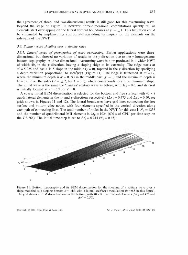
3.3.1. Lateral speed of propagation of wa6e o6erturning. Earlier applications were three-dimensional but showed no variation of results in the y-direction due to the y-homogeneousbottom topography. A three-dimensional overturning wave is now produced in a wider NWTof width 4h0 in the y-direction, having a sloping ridge at its extremity. The ridge starts atx %=5.225 and has a 1:15 slope in the middle (y=0), tapered in the y-direction by specifyinga depth variation proportional to sech2(ky) (Figure 11). The ridge is truncated at x %=19,where the minimum depth is h %=0.093 in the middle part (y %=0) and the maximum depth ish %=0.619 on the sides (y %=92, for k=0.5), which corresponds to a 1:36 minimum slope.The initial wave is the same the ‘Tanaka’ solitary wave as before, with H %0=0.6, and its crestis initially located at x %=5.7 for t %=0.
A coarse initial BEM discretization is selected for the bottom and free surface, with 40×8quadrilateral elements in the x- and y-directions respectively (Dx %0=0.475 and Dy %0=0.50; seegrids shown in Figures 11 and 12). The lateral boundaries have grid lines connecting the freesurface and bottom edge nodes, with four elements specified in the vertical direction alongeach pair of connecting lines. The total number of nodes in the NWT for this case is NG=1238and the number of quadrilateral MII elements is MG=1024 (600 s of CPU per time step onthe G3-266). The initial time step is set to Dt %0=0.214 (C0=0.45).
Figure 11. Bottom topography and its BEM discretization for the shoaling of a solitary wave over aridge modeled as a sloping bottom s=1:15, with a lateral sech2(ky) modulation (k=0.5 in this figure).The grid shows a BEM discretization on the bottom, with 40×8 quadrilateral elements (Dx0%=0.475 and
Dy0%=0.50).
Copyright © 2001 John Wiley & Sons, Ltd. Int. J. Numer. Meth. Fluids 2001; 35: 829–867

S. T. GRILLI, P. GUYENNE, AND F. DIAS858
Figure 12. Free surface shape at t %=6.00 for the propagation of an exact solitary wave of heightH0%=0.6 over a ridge (see Figure 11) in a 3D-NWT with 40×8 quadrilateral elements on the free surface
(initial discretization). The wave crest is located at x %=5.7 for t %=0.
In this application, wave overturning eventually occurs and leads to a large increase innumerical errors, due to the strong convergence of nodes and the gradual loss of accuracy ofnumerical integrations in the overturning jet. (This is similar to results obtained in the2D-NWT by Grilli and Subramanya [22].) In the analyses, results will be deemed acceptablewhen numerical errors are less than 1 per cent. Computations will first be performed in theinitial discretization up to reaching these maximum errors (t %58.788). To refine the BEMdiscretization resolution in the region where wave overturning occurs, without an unnecessarylarge increase in the total number of nodes, regridding of the extremity of the NWT to a finerdiscretization will be performed for results obtained at an earlier time, when errors are verysmall (t %=6.000) and computations restarted up to again reaching the maximum errors.
Figure 12 shows results of computations in the initial discretization after 51 time steps, att %=6.000, corresponding to the stage at which regridding is specified. At this time, numericalerrors on wave mass and energy conservation are quite small, with om=0.065 per cent andoe=0.045 per cent. Figure 13 shows results obtained after 103 time steps in the samediscretization (t %=8.788). At this time, numerical errors are om=0.248 per cent and oe=0.865per cent, i.e., close to the admissible maximum value for the latter one. Due to the nodeconvergence at the wave crest, the time step has reduced to Dt %=0.0096. The wave haspropagated to the far right of the NWT, and its front part starts overturning in the middleshallower part of the tank (y %=0), with H %=0.700 at x %=17.010.
Regridding is applied at t %=6.000, when the wave crest is located at x %=14.203 andH %=0.644, i.e., much before the wave starts overturning (Figure 12). The discretization isincreased to 40×10 quadrilateral elements on the free surface and bottom boundaries, forx %=8.075–19, and nodes are regridded to constant intervals (with Dx %0=0.273 and Dy %0=0.40). The total number of nodes in the NWT is now NG=1422 and the number ofquadrilateral MII elements is MG=1200 (735 s of CPU per time step on the G3-266). Theinitial time step after regridding is set to Dt %=0.123 (C0=0.45). Figure 14 shows the wavecomputed after 130 time steps in the regridded discretization at t %=9.196; the final time stephas reduced to Dt %=0.0051. At this stage, the error on wave energy conservation reaches the
Copyright © 2001 John Wiley & Sons, Ltd. Int. J. Numer. Meth. Fluids 2001; 35: 829–867

3D OVERTURNING WAVES OVER AN ARBITRARY BOTTOM 859
Figure 13. Same case as in Figures 11 and 12. Wave shape calculated at t %=8.788 in the initialdiscretization (3D-NWT with 40×8 quadrilateral elements on the free surface for x %]0).
maximum, with oe=1.012 per cent and om=0.164 per cent. In fact, overturning has alreadyreached the NWT sidewalls (y %=92), on which elements start wrapping; hence, computationscannot be pursued much beyond this stage. (This limitation again could be eliminated by eitherusing proper regridding on the sidewall boundaries or by using an even wider NWT, in whichwave overturning would occur for a longer time in the middle part of the wave, beforereaching the sidewalls; see next application.) Comparing Figures 13 and 14 we see that byusing regridding, wave overturning is both calculated for a longer time and with a finerresolution within the same maximum numerical errors.
Figure 14. Same case as in Figures 11 and 12. Wave shape calculated at t %=9.196 in the regriddeddiscretization (3D-NWT with 40×10 quadrilateral elements on the free surface for x %]8.075).
Copyright © 2001 John Wiley & Sons, Ltd. Int. J. Numer. Meth. Fluids 2001; 35: 829–867
S. T. GRILLI, P. GUYENNE, AND F. DIAS860
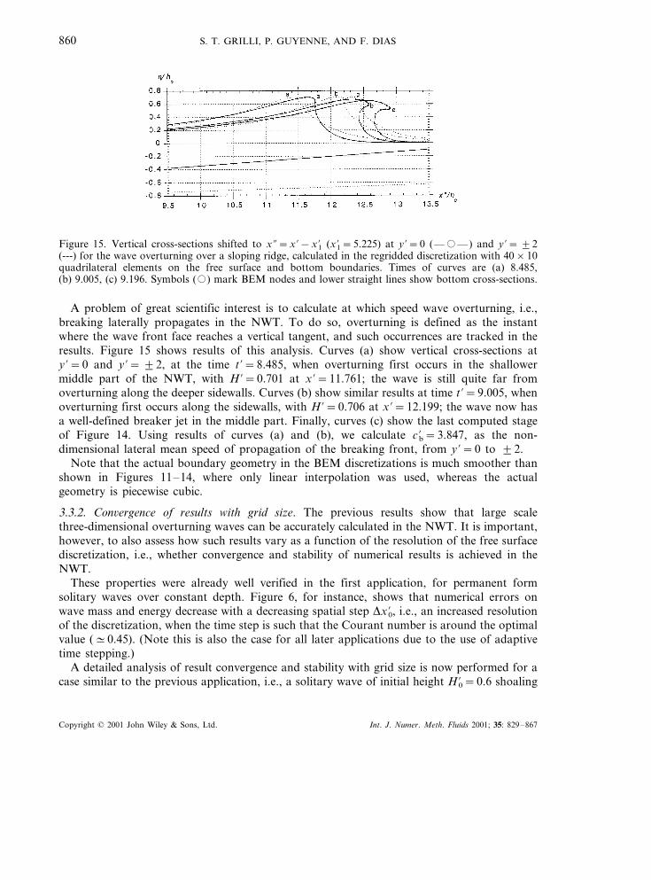
Figure 15. Vertical cross-sections shifted to x¦=x %−x1% (x1%=5.225) at y %=0 (—�—) and y %=92(---) for the wave overturning over a sloping ridge, calculated in the regridded discretization with 40×10quadrilateral elements on the free surface and bottom boundaries. Times of curves are (a) 8.485,(b) 9.005, (c) 9.196. Symbols (�) mark BEM nodes and lower straight lines show bottom cross-sections.
A problem of great scientific interest is to calculate at which speed wave overturning, i.e.,breaking laterally propagates in the NWT. To do so, overturning is defined as the instantwhere the wave front face reaches a vertical tangent, and such occurrences are tracked in theresults. Figure 15 shows results of this analysis. Curves (a) show vertical cross-sections aty %=0 and y %=92, at the time t %=8.485, when overturning first occurs in the shallowermiddle part of the NWT, with H %=0.701 at x %=11.761; the wave is still quite far fromoverturning along the deeper sidewalls. Curves (b) show similar results at time t %=9.005, whenoverturning first occurs along the sidewalls, with H %=0.706 at x %=12.199; the wave now hasa well-defined breaker jet in the middle part. Finally, curves (c) show the last computed stageof Figure 14. Using results of curves (a) and (b), we calculate c %b=3.847, as the non-dimensional lateral mean speed of propagation of the breaking front, from y %=0 to 92.
Note that the actual boundary geometry in the BEM discretizations is much smoother thanshown in Figures 11–14, where only linear interpolation was used, whereas the actualgeometry is piecewise cubic.
3.3.2. Con6ergence of results with grid size. The previous results show that large scalethree-dimensional overturning waves can be accurately calculated in the NWT. It is important,however, to also assess how such results vary as a function of the resolution of the free surfacediscretization, i.e., whether convergence and stability of numerical results is achieved in theNWT.
These properties were already well verified in the first application, for permanent formsolitary waves over constant depth. Figure 6, for instance, shows that numerical errors onwave mass and energy decrease with a decreasing spatial step Dx %0, i.e., an increased resolutionof the discretization, when the time step is such that the Courant number is around the optimalvalue (#0.45). (Note this is also the case for all later applications due to the use of adaptivetime stepping.)
A detailed analysis of result convergence and stability with grid size is now performed for acase similar to the previous application, i.e., a solitary wave of initial height H %0=0.6 shoaling
Copyright © 2001 John Wiley & Sons, Ltd. Int. J. Numer. Meth. Fluids 2001; 35: 829–867
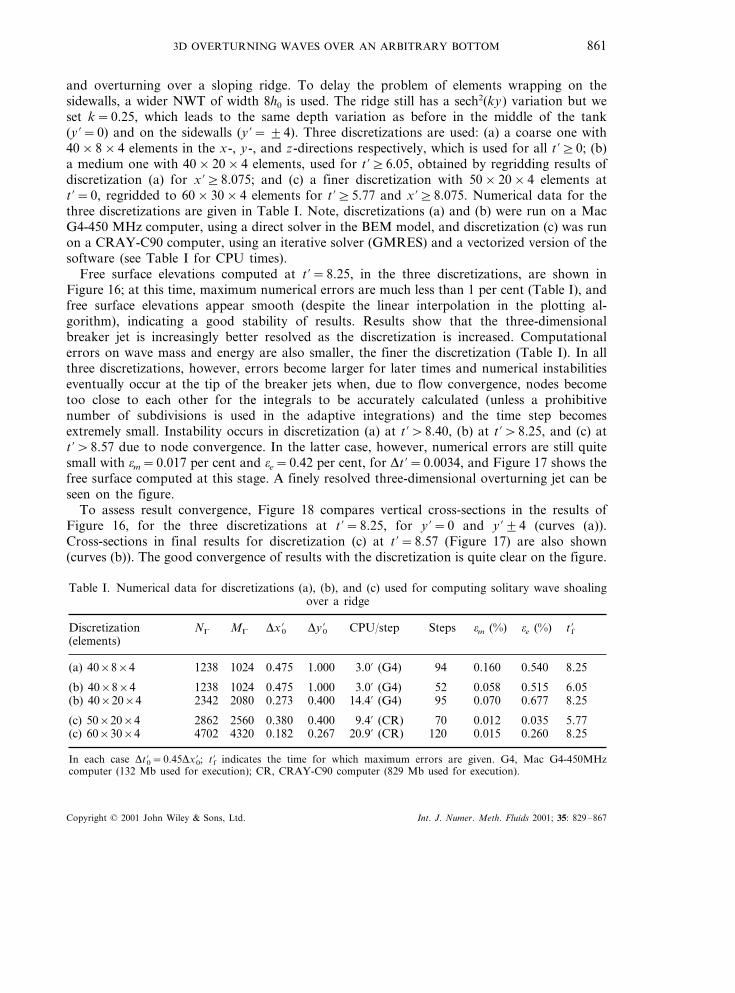
3D OVERTURNING WAVES OVER AN ARBITRARY BOTTOM 861
and overturning over a sloping ridge. To delay the problem of elements wrapping on thesidewalls, a wider NWT of width 8h0 is used. The ridge still has a sech2(ky) variation but weset k=0.25, which leads to the same depth variation as before in the middle of the tank(y %=0) and on the sidewalls (y %=94). Three discretizations are used: (a) a coarse one with40×8×4 elements in the x-, y-, and z-directions respectively, which is used for all t %]0; (b)a medium one with 40×20×4 elements, used for t %]6.05, obtained by regridding results ofdiscretization (a) for x %]8.075; and (c) a finer discretization with 50×20×4 elements att %=0, regridded to 60×30×4 elements for t %]5.77 and x %]8.075. Numerical data for thethree discretizations are given in Table I. Note, discretizations (a) and (b) were run on a MacG4-450 MHz computer, using a direct solver in the BEM model, and discretization (c) was runon a CRAY-C90 computer, using an iterative solver (GMRES) and a vectorized version of thesoftware (see Table I for CPU times).
Free surface elevations computed at t %=8.25, in the three discretizations, are shown inFigure 16; at this time, maximum numerical errors are much less than 1 per cent (Table I), andfree surface elevations appear smooth (despite the linear interpolation in the plotting al-gorithm), indicating a good stability of results. Results show that the three-dimensionalbreaker jet is increasingly better resolved as the discretization is increased. Computationalerrors on wave mass and energy are also smaller, the finer the discretization (Table I). In allthree discretizations, however, errors become larger for later times and numerical instabilitieseventually occur at the tip of the breaker jets when, due to flow convergence, nodes becometoo close to each other for the integrals to be accurately calculated (unless a prohibitivenumber of subdivisions is used in the adaptive integrations) and the time step becomesextremely small. Instability occurs in discretization (a) at t %\8.40, (b) at t %\8.25, and (c) att %\8.57 due to node convergence. In the latter case, however, numerical errors are still quitesmall with om=0.017 per cent and oe=0.42 per cent, for Dt %=0.0034, and Figure 17 shows thefree surface computed at this stage. A finely resolved three-dimensional overturning jet can beseen on the figure.
To assess result convergence, Figure 18 compares vertical cross-sections in the results ofFigure 16, for the three discretizations at t %=8.25, for y %=0 and y %94 (curves (a)).Cross-sections in final results for discretization (c) at t %=8.57 (Figure 17) are also shown(curves (b)). The good convergence of results with the discretization is quite clear on the figure.
Table I. Numerical data for discretizations (a), (b), and (c) used for computing solitary wave shoalingover a ridge
Discretization t %fNG MG Dx %0 Dy %0 CPU/step Steps om (%) oe (%)(elements)
8.25(a) 40×8×4 1238 1024 0.475 1.000 3.0% (G4) 94 0.160 0.540
0.515(b) 40×8×4 6.051238 1024 0.475 1.000 3.0% (G4) 52 0.0588.250.6770.07095(b) 40×20×4 14.4% (G4)0.4000.27320802342
0.012 0.035 5.77(c) 50×20×4 2862 2560 0.380 0.400 9.4% (CR) 700.18243204702 8.250.2600.01512020.9% (CR)(c) 60×30×4 0.267
In each case Dt %0=0.45Dx %0; t %f indicates the time for which maximum errors are given. G4, Mac G4-450MHzcomputer (132 Mb used for execution); CR, CRAY-C90 computer (829 Mb used for execution).
Copyright © 2001 John Wiley & Sons, Ltd. Int. J. Numer. Meth. Fluids 2001; 35: 829–867
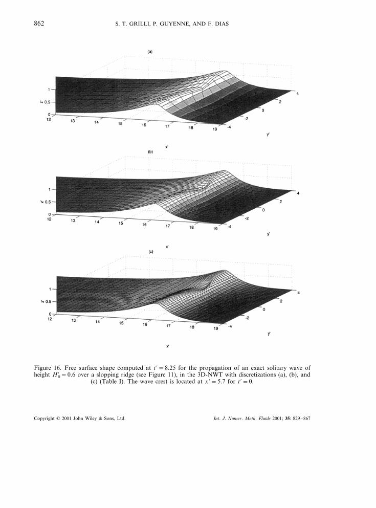
S. T. GRILLI, P. GUYENNE, AND F. DIAS862
Figure 16. Free surface shape computed at t %=8.25 for the propagation of an exact solitary wave ofheight H0%=0.6 over a slopping ridge (see Figure 11), in the 3D-NWT with discretizations (a), (b), and
(c) (Table I). The wave crest is located at x %=5.7 for t %=0.
Copyright © 2001 John Wiley & Sons, Ltd. Int. J. Numer. Meth. Fluids 2001; 35: 829–867
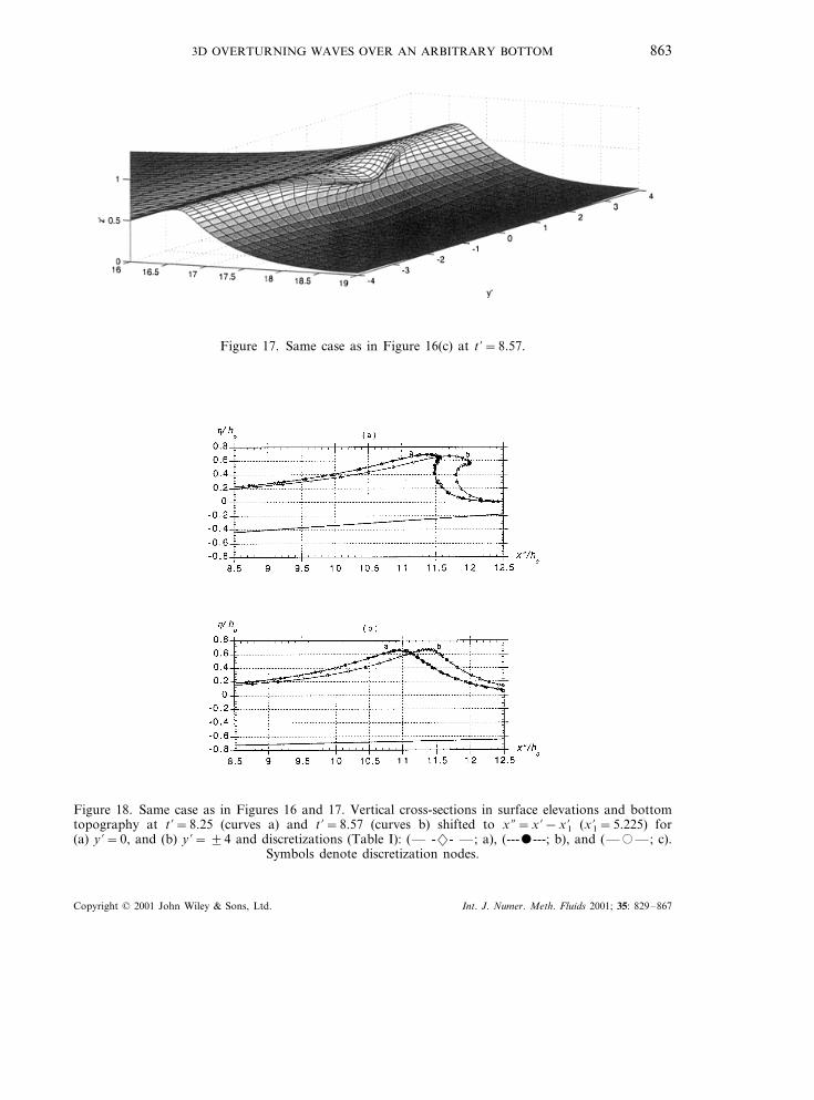
3D OVERTURNING WAVES OVER AN ARBITRARY BOTTOM 863
Figure 17. Same case as in Figure 16(c) at t %=8.57.
Figure 18. Same case as in Figures 16 and 17. Vertical cross-sections in surface elevations and bottomtopography at t %=8.25 (curves a) and t %=8.57 (curves b) shifted to x¦=x %−x1% (x1%=5.225) for(a) y %=0, and (b) y %=94 and discretizations (Table I): (— -2- —; a), (------; b), and (—�—; c).
Symbols denote discretization nodes.
Copyright © 2001 John Wiley & Sons, Ltd. Int. J. Numer. Meth. Fluids 2001; 35: 829–867

S. T. GRILLI, P. GUYENNE, AND F. DIAS864
All results agree well with each other, particularly in the back of the wave and in theoverturning jet. Even the very coarse discretization (a) is able to predict quite well the shapeof the overturning wave. Curves (b) show how nodes/elements become very dense at the wavecrest and in the breaker jet, eventually leading to quasi-singularities in the integrations.
4. CONCLUSIONS
An accurate and efficient 3D-NWT was developed, implemented, and tested. Overall, resultsobtained in this study show a better stability and numerical accuracy than in previous attemptsreported in the literature of calculating such strongly non-linear three-dimensional surfacewaves. Large scale wave overturning over arbitrary bottom topography is calculated which, toour knowledge, was never successfully achieved in a general 3D-NWT. An interesting physicalresult is the speed of lateral propagation of wave breaking; this will be further investigated infuture studies.
More specifically, in the reported applications, global accuracy of computations in terms ofconservation of wave mass and energy is always very good and the computed wave shapeconverges well with the grid size, particularly in the overturning region. No numericalproblems are experienced at boundary intersections (corners/edges) of the computationaldomain (e.g., as in Romate [34]), nor are sawtooth instabilities observed at the grid wave-length, with growing time. No smoothing is thus required to stabilize the solution (e.g., as inXu and Yue [35,36]). When regridding is used, it is simply to introduce more nodes/fluidparticles in selected areas of the free surface, to provide more resolution; the solution at thecurrent time step is simply reinterpolated but not modified and hence this does not constitutesmoothing (i.e., filtering). Different interpolation methods are used for the BEM computationsand for calculating the tangential derivatives required for time stepping, but this does notconstitute (explicit) smoothing either. Note only a few hundred time steps were run in the3D-NWT for these applications, but similarly accurate and stable results were observed inGrilli et al.’s 2D-NWT, which is based on similar algorithms, for computations coveringseveral thousands of time steps.
As in earlier two-dimensional applications [18,22,46], which showed similar accuracy andstability properties, we believe that the accuracy and stability of the three-dimensional modelresults from both the higher-order BEM method, with C2 local inter-element continuity, whichensures a very accurate solution of Laplace’s equation at every time step, and the explicit timestepping method based on second-order Taylor series, which include higher-order spatialderivatives to calculate the new position of a node at the next time step. This method had beenshown in two dimensions to be more stable, accurate, and efficient than predictor–correctormethods, which simply extrapolate the position of each node, based on earlier locations on itsown trajectory, without any effect of neighboring nodes (i.e., spatial variations); this moreeasily leads to sawtooth instabilities. We find that the same holds true for the three-dimen-sional model. As pointed out by Xu and Yue [36], such strongly non-linear surface waveproblems require very accurate numerical methods in all respects, to prevent errors fromgrowing in time, through non-linear interactions, and leading to the numerical instability of thesolution. Here, even after almost 200 time steps (last application) no significant error isobserved for mass and energy conservation, without need for smoothing the solution.
Copyright © 2001 John Wiley & Sons, Ltd. Int. J. Numer. Meth. Fluids 2001; 35: 829–867

3D OVERTURNING WAVES OVER AN ARBITRARY BOTTOM 865
Finally, as mentioned before, these are quite demanding numerical computations. In thepresent study, the focus was on developing and validating the 3D-NWT and no specificattempt was made to optimize the solution for very large problems, such as dividing thedomain in sub-regions (Wang et al. [50]), except that the more efficient GMRES iterativesolver was used for the larger BEM systems of equations (as, e.g., in Xu and Yue [35,36] orFerrant [39]) and the software code was optimized for the CRAY-C90 supercomputer. Itshould be pointed out, however, that with the ever increasing power of microprocessors, evenproblems with fairly large discretization sizes can still be run on desktop computers. Forinstance, many of the computations reported in this paper were performed on a laptop MacPowerPC G3 computer (266 MHz, 64 Mb of RAM), on which the largest problem, with 1422nodes, took about 12.25 min of CPU per time step and 49 Mb of RAM. Even larger problemswere run on a Mac PowerPC G4 computer (450 MHz, 1 Gb of RAM), which turned out tobe 3–4 times faster than the G3 and about half as fast as the CRAY-C90; the largest problemrun on the G4 had 2342 nodes and took about 14.40 min of CPU per time step and 132 Mbof RAM. Since the computation time using the iterative solver and the NWT memoryrequirement both grow with the power 2 or so of the number of nodes NG, it is anticipated thatwith the present implementation of the model a problem with 6400 nodes could be run on theG4 computer, using about 950 Mb of RAM and 105 min CPU per time step. For even largerthree-dimensional problems, much more important computer resources and/or use of optimiz-ing techniques would be required. Clearly, even with faster algorithms, such computationswould require a supercomputer such as the CRAY-C90 or even a massively parallelsupercomputer.
It is anticipated that a fully optimized and vectorized/parallelized 3D-NWT will make itpossible to efficiently perform very large size computations, thus providing a great wealth ofnew insight into the physics of three-dimensional breaking waves.
ACKNOWLEDGMENTS
This publication is the result of research sponsored by the ‘Centre National de la Recherche Scientifique’(CNRS, France). Support to the first author, provided by the Institut Non-Lineaire de Nice, UMR 6618CNRS-UNSA, while he was on sabbatical leave in France, is gratefully acknowledged, as well as a grantfrom the US Office of Naval Research (N-00014-99-10439 of the Coastal Dynamics Division; code 321CD). The second and third authors acknowledge support from the Delegation Generale de l’Armement.The computations presented in this work were performed in part on the CRAY-C90 supercomputerlocated at IDRIS (Institut du Developpement et des Resources en Informatique Scientifique, France),and were funded by the CNRS.
REFERENCES
1. Mei CC. The Applied Dynamics of Ocean Surface Wa6es (2nd edn). World Scientific: New Jersey, 1989.2. Wei J, Kirby JT, Grilli ST, Subramanya R. A fully nonlinear Boussinesq model for surface waves. I. Highly
nonlinear unsteady waves. Journal of Fluid Mechanics 1995; 294: 71–92.3. Dommermuth DG, Yue DKP, Lin WM, Rapp RJ, Chan ES, Melville WK. Deep-water plunging breakers: a
comparison between potential theory and experiments. Journal of Fluid Mechanics 1988; 189: 423–442.4. Skyner D. A comparison of numerical predictions and experimental measurements of the internal kinematics of
a deep-water plunging wave. Journal of Fluid Mechanics 1996; 315: 51.
Copyright © 2001 John Wiley & Sons, Ltd. Int. J. Numer. Meth. Fluids 2001; 35: 829–867

S. T. GRILLI, P. GUYENNE, AND F. DIAS866
5. Grilli ST, Subramanya R, Svendsen IA, Veeramony J. Shoaling of solitary waves on plane beaches. Journal ofWaterways, Port, Coastal and Ocean Engineering 1994; 120(6): 609–628.
6. Grilli ST, Svendsen IA, Subramanya R. Breaking criterion and characteristics for solitary waves on plane beaches.Journal of Waterways, Port, Coastal and Ocean Engineering 1997; 123(3): 102–112.
7. Li Y, Raichlen F. Breaking criterion and characteristics for solitary waves on slopes—Discussion. Journal ofWaterways, Port, Coastal and Ocean Engineering 1998; 124(6): 329–333.
8. Grilli ST. Free surface nonlinear flows. In 1999 McGraw-Hill Yearbook of Sciences and Technology (a yearlysupplement to the Encyclopedia of Sciences and Technology), Parker SP (ed.). McGraw-Hill: New York, 1997;134–136.
9. Guignard S, Marcer R, Rey V, Kharif C, Fraunie Ph. Solitary wave breaking on sloping beaches: 2D two-phaseflow numerical simulation by SL-VOF method. European Journal of Mechanics B/Fluids 2001 (accepted).
10. Chen G, Kharif C, Zaleski S, Li J. Two-dimensional Navier–Stokes simulation of breaking waves. Physics andFluids 1999; 111: 121–133.
11. Guignard S, Grilli ST, Marcer R, Rey V. Computation of shoaling and breaking waves in nearshore areas by thecoupling of BEM and VOF methods. In Proceedings of the 9th International Offshore and Polar EngineeringConference (ISOPE99), Brest, France, May, vol. III, Chung JS, Olagnon M, Kim CH, Francescutto A (eds).International Society of Offshore and Polar Engineers: Cupertino 1999; 304–309.
12. Brebbia CA. The Boundary Element Method for Engineers. Wiley: New York, 1978.13. Longuet-Higgins MS, Cokelet ED. The deformation of steep surface waves on water—I. A numerical method of
computation. Proceedings of the Royal Society London 1976; A350: 1–26.14. Dold JW, Peregrine DH. An efficient boundary integral method for steep unsteady water waves. In Numerical
Methods for Fluid Dynamics II, Morton KW, Baines MJ (eds). Clarendon Press: Oxford, 1986; 671–679.15. Vinje T, Brevig P. Numerical simulation of breaking waves. Ad6ances in Water Research 1981; 4: 77–82.16. New AL, McIver P, Peregrine DH. Computation of overturning waves. Journal of Fluid Mechanics 1985; 150:
233–251.17. Klopman G. Numerical simulation of gravity wave motion on steep slopes. Delft Hydraulics Report No. H195,
1988.18. Grilli ST, Skourup J, Svendsen IA. An efficient boundary element method for nonlinear water waves. Engineering
Analysis with Boundary Elements 1989; 6(2): 97–107.19. Cointe R. Numerical simulation of a wave channel. Engineering Analysis with Boundary Elements 1990; 7(4):
167–177.20. Cooker MJ. A boundary-integral method for water wave motion over irregular bed. Engineering Analysis with
Boundary Elements 1990; 7(4): 205–213.21. Ohyama T, Nadaoka K. Development of a numerical wave tank for analysis of nonlinear and irregular wave
fields. Fluid Dynamics Research 1991; 8: 231–251.22. Grilli ST, Subramanya R. Numerical modeling of wave breaking induced by fixed or moving boundaries.
Computational Mechanics 1996; 17: 374–391.23. Grilli ST, Horrillo J. Numerical generation and absorption of fully nonlinear periodic waves. Journal of
Engineering Mechanics 1997; 123(10): 1060–1069.24. Dommermuth DG, Yue DKP. Numerical simulation of nonlinear axisymmetric flows with a free surface. Journal
of Fluid Mechanic 1987; 178: 195–219.25. Forbes LK. An algorithm for three-dimensional free-surface problems in hydrodynamics. Journal of Computa-
tional Physics 1989; 82(2): 330–347.26. Boo SY. Application of higher-order boundary element method to steady ship wave problem and time domain
simulation of nonlinear gravity waves. PhD dissertation, Ocean Engineering Progress, Texas A&M University,1993.
27. Lee CC, Liu YH, Kim CH. Simulation of nonlinear waves and forces due to transient and steady motion of asubmerged sphere. International Journal of Offshore and Polar Engineering 1994; 4(3): 174–182.
28. Isaacson M, de St. Q. Nonlinear effects on fixed and floating bodies. Journal of Fluid Mechanics 1982; 120:267–281.
29. Yang C, Ertekin RC. Numerical simulation of nonlinear wave diffraction by a vertical cylinder. Journal ofOffshore Mechanics and Arctic Engineering 1992; 114: 36–44.
30. Cheung KF, Isaacson M, Lee JW. Wave diffraction around a three-dimensional body in a current. Journal ofOffshore Mechanics and Arctic Engineering 1996; 118(4): 247–252.
31. Lalli F, Di Mascio A, Landrini M. Nonlinear diffraction effects around a surface-piercing structure. InternationalJournal of Offshore and Polar Engineering 1996; 6(2): 104–111.
32. Celebi MS, Kim MH, Beck RF. Fully nonlinear 3D numerical wave tank simulations. Journal of Ship Research1998; 42(1): 33–45.
Copyright © 2001 John Wiley & Sons, Ltd. Int. J. Numer. Meth. Fluids 2001; 35: 829–867
3D OVERTURNING WAVES OVER AN ARBITRARY BOTTOM 867
33. Ferrant P. Runup on a cylinder due to waves and currents: potential flow solution with fully nonlinear boundaryconditions. In Proceedings of the 8th International Offshore and Polar Engineering Conference, Montreal, vol. 3,Chung JS, Olagnon M, Kim CH, Koterayama W (eds). International Society of Offshore and Polar Engineers:Cupertino, 1998; 332–339.
34. Romate JE. The numerical simulation of nonlinear gravity waves in three dimensions using a higher order panelmethod. PhD dissertation, Department of Applied Mathematics, University of Twente, The Netherlands, 1989.
35. Xu H, Yue DKP. Numerical study of three dimensional overturning waves. In Proceedings of the 7th InternationalWorkshop on Water Wa6es and Floating Bodies, Cointe R (ed.). Val de Reuil, France, May, Fluid Flow andComputational Aspects, 1992; 303–307.
36. Xu H, Yue DKP. Computations of fully-nonlinear three-dimensional water waves. In Proceedings of the 19thSymposium on Na6al Hydrodynamics, Seoul, Korea, August, 1992.
37. Broeze J. Numerical modelling of nonlinear free surface waves with a 3D panel method. PhD dissertation,Enschede, The Netherlands, 1993.
38. Boo SY, Kim CH, Kim MH. A numerical wave tank for nonlinear irregular waves by 3D higher-order boundaryelement method. International Journal of Offshore and Polar Engineering 1994; 4(4): 265–272.
39. Ferrant P. Time domain computation of nonlinear diffraction loads upon three-dimensional floating bodies. InProceedings of the 5th International Offshore and Polar Engineering Conference, The Hague, vol. 3, Chung JS,Olagnon M, Koterayama W (eds). International Society of Offshore and Polar Engineers: Cupertino, 1995;280–288.
40. Yeung RW. Numerical methods in free surface flows. Annual Re6iew in Fluid Mechanics 1982; 14: 395–442.41. Peregrine DH. Breaking waves on beaches. Annual Re6iew of Fluid Mechanics 1983; 15: 149–178.42. Grilli ST. Modeling of nonlinear wave motion in shallow water. In Computational Methods for Free and Mo6ing
Boundary Problems in Heat and Fluid Flow, Wrobel LC, Brebbia CA (eds). Computational Mechanics Publisher,Elsevier Applied Science: London, 1993; 37–65.
43. Grilli ST, Subramanya R. Recent advances in the BEM modelling of nonlinear water waves. In Boundary ElementApplications in Fluid Mechanics. Ad6ances in Fluid Mechanics Series, Power H (ed.). Computational MechanicsPublishers: Southampton, 1995; 91–122.
44. Tsai WT, Yue DKP. Computation of nonlinear free-surface flows. Annual Re6iew of Fluid Mechanics 1996; 28:249–278.
45. Kim CH, Clement AH, Tanizawa K. Recent research and development of numerical wave tank—a review.International Journal of Offshore and Polar Engineering 1999; 9(4): 241–256.
46. Grilli ST, Svendsen IA. Corner problems and global accuracy in the boundary element solution of nonlinear waveflows. Engineering Analysis with Boundary Elements 1990; 7(4): 178–195.
47. Grilli ST, Subramanya R. Quasi-singular integrals in the modeling of nonlinear water waves in shallow water.Engineering Analysis with Boundary Elements 1994; 13(2): 181–191.
48. Badmus T, Cheng AH-D, Grilli ST. A three-dimensional Laplace transform BEM for poroelasticity. InternationalJournal for Numerical Methods in Engineering 1993; 36: 67–85.
49. Tanaka M. The stability of solitary waves. Physics and Fluids 1986; 29(3): 650–655.50. Wang P, Yao Y, Tulin MP. An efficient numerical tank for nonlinear water waves based on the multi-subdomain
approach with BEM. International Journal of Numerical Methods in Fluids 1995; 20: 1315–1336.
Copyright © 2001 John Wiley & Sons, Ltd. Int. J. Numer. Meth. Fluids 2001; 35: 829–867