A Fourth Order Accurate Discretization for the

Laplace and Heat Equations on Arbitrary Domains,

with Applications to the Stefan Problem ∗

Frederic Gibou† Ronald Fedkiw ‡

April 27, 2004

Abstract

In this paper, we first describe a fourth order accurate finite differ-ence discretization for both the Laplace equation and the heat equationwith Dirichlet boundary conditions on irregular domains. In the caseof the heat equation we use an implicit time discretization to avoid thestringent time step restrictions associated with explicit schemes. Wethen turn our focus to the Stefan problem and construct a third or-der accurate method that also includes an implicit time discretization.Multidimensional computational results are presented to demonstratethe order accuracy of these numerical methods.

∗Research supported in part by an ONR YIP and PECASE award (N00014-01-1-0620),a Packard Foundation Fellowship, a Sloan Research Fellowship, ONR N00014-03-1-0071,ONR N00014-02-1-0720, NSF DMS-0106694 and NSF ACI-0323866. In addition, the firstauthor was supported in part by an NSF postdoctoral fellowship (DMS-0102029).

†Mathematics Department & Computer Science Department, Stanford University,Stanford, CA 94305.

‡Computer Science Department, Stanford University, Stanford, CA 94305.

1

1 Introduction

Various numerical methods have been developed to solve the Stefan prob-lem. These methods need to be able to efficiently solve the heat equation onirregular domains and keep track of a moving interface that may undergocomplex topological changes. The interface that separates the two phasescan be either explicitly tracked or implicitly captured. The main disadvan-tage of an explicit approach, e.g. front tracking (see e.g. [16]), is that specialcare is needed for topological changes such as merging or breaking. More-over, the explicit treatment of connectivity makes the method challengingto extend to three spatial dimensions. Implicit representations such as thelevel set method [24, 30] or the phase-field method [17] embed the front as anisocontour of a continuous function. Topological changes are consequentlyhandled in a straightforward fashion, and thus these methods are readilyimplemented in both two and three spatial dimensions.

Phase-field methods represent the front implicitly and have producedimpressive three dimensional results (see e.g. [17, 7]). However, these meth-ods only have an approximate representation of the front location, and thusthe discretization of the diffusion field is less accurate near the front resem-bling an enthalpy method [5]. Moreover, it is often challenging to add newphysics to the model since new asymptotic analysis is often required. Formore details on phase field methods for the Stefan problem, see [17] and thereferences therein.

In this paper, we employ the sharp interface implicit representation ofthe level set method [24, 30]. The earliest level set method for solidificationtype problems was presented in [31] where the authors recast the equationsof motion into a boundary integral equation and used the level set methodto update the location of the interface. In [2], the boundary integral equa-tions were avoided by using a finite difference method to solve the diffusionequation on a Cartesian grid with Dirichlet boundary conditions imposedon the interface. The jump in the first derivatives of the temperature wasused to compute an interface velocity that was extended to a band about theinterface and used to evolve the level set function in time. [10] showed thatthis discretization produces results in accordance with solvability theory. In[35], the authors discretized the heat equation on a Cartesian grid in a man-ner quite similar to that proposed in [2] resulting in a nonsymmetric linearsystem when applying implicit time discretization. [35] used front trackingto update the location of the interface improving upon the front trackingapproach proposed in [16] which used the smeared out immersed boundarymethod [25] and an explicit time discretization.

2

In [15], the authors solved a variable coefficient Poisson equation in thepresence of an irregular interface where Dirichlet boundary conditions wereimposed. They used a finite volume method that results in a nonsymmetricdiscretization matrix. Both multigrid methods and adaptive mesh refine-ment were used, and in [14] this nonsymmetric discretization was coupledto a volume of fluid front tracking method in order to solve the Stefan prob-lem. In [27] the authors used adaptive finite element methods for both theheat equation and for the interface evolution producing stunning three di-mensional results. Other remarkable three dimensional results can be foundin the finite difference diffusion Monte Carlo method of [26]. Recently, [36]formulated a second order accurate method for the Stefan problem in twospatial dimensions using a Galerkin finite element approach to solve for theenergy equation. In this work, the interface was tracked with a set of markerparticles making the method potentially hard to extend to three spatial di-mensions. Moreover, the velocity was computed under the assumption thatthe interface cuts the element in a straight line. The interested reader isreferred to [16], [2], [8] and the references therein for an extensive summaryof computational results for the Stefan problem.

Standard convergence proofs use stability and consistency analysis toimply convergence, i.e. given stability, a sufficient condition for a scheme tobe pth order accurate is that the local truncation error is pth order. However,a pth order local truncation error is not a necessary condition and one canderive pth order accurate schemes despite the fact that their local truncationerror is of lower order. [23] (see also [19]) made this point in the contextof second order, scalar boundary value problems on nonuniform meshes. Infact, in the process of constructing second order accurate methods for suchproblems, many authors had unnecessarily focused on imposing special re-strictions on the mesh size in order to obtain a second order accurate localtruncation error, see e.g [4, 11]. In the case of our present work, authors havealso been misled by the limitation of standard convergence analysis proofsand have proposed unnecessarily complex schemes. For example, in [2] (seealso [10]) the authors approximate the Laplace operator with the standardsecond order accurate central scheme limiting the overall solution to secondorder accuracy. However, their discretization of the Laplace operator forgrid nodes neighboring the interface amounts to differentiating a quadraticinterpolant of the temperature twice in each spatial dimension. [9] refor-mulated the interface treatment with the use of ghost cells (based on theghost fluid method [6]) defined by extrapolation of the temperature acrossthe interface, and showed that local linear extrapolation is enough to obtainsecond order spatial accuracy for both the Laplace and heat equations on

3

irregular domains. Moreover, their discretization had the added benefit ofyielding a symmetric linear system as opposed to the nonsymmetric systemin [2]. This scheme served as the basis of a simple method to solve the Stefanproblem. It was further used in [8] to show that one could obtain solutions inagreement with solvability theory, and could simulate many of the physicalfeatures of crystal growth such as molecular kinetics and surface tension.

In this paper, we exploit the methodology of [9] to derive a fourth orderaccurate finite difference discretization for the Laplace equation on irregulardomains. Then we apply this framework to derive a fourth order accuratediscretization for the heat equation with Dirichlet boundary conditions onarbitrary domains. In this case we use an implicit time discretization toavoid the stringent time step restrictions induced by explicit schemes. Wethen turn our focus to the Stefan problem with Dirichlet boundary con-ditions and construct a third order accurate discretization that includesimplicit integration in time. Multidimensional computational results arepresented to verify the order accuracy of these numerical methods.

2 Laplace Equation

Consider a Cartesian computational domain, Ω ⊂ Rn, with exterior bound-ary, ∂Ω, and a lower dimensional interface, Γ, that divides the computationaldomain into disjoint pieces, Ω− and Ω+. The Laplace equation is given by

4T (~x) = f(~x), ~x ∈ Ω−, (1)

where ~x = (x, y, z) is the vector of spatial coordinates, 4 = ∂2

∂x2 + ∂2

∂y2 + ∂2

∂z2 isthe Laplace operator, and T is assumed to be smooth on Ω−. On Γ, Dirichletboundary conditions are specified. To separate the different domains, weintroduce a level set function φ defined as:

φ < 0 for ~x ∈ Ω−,φ > 0 for ~x ∈ Ω+,φ = 0 for ~x ∈ Γ.

A convenient choice that ensures numerical robustness is to define φ as thesigned distance function to the interface. The level set function is also usedto identify the location of the interface to high order accuracy as will bediscussed throughout this paper.

The discretization of the Laplace operator, including the special treat-ments needed at the interface, is performed in a dimension by dimensionfashion. Therefore, without loss of generality, we first describe the dis-cretization in one spatial dimension.

4

2.1 1D Laplace Equation

Consider the Laplace equation in one spatial dimension, i.e. Txx = f . Thecomputational domain is discretized into cells of size4x with the grid nodesxi located at their centers. The solution to the Laplace equation is computedat the grid nodes and is written as Ti = T (xi). We consider the standardfourth order discretization:

(Txx)i ≈− 1

12Ti−2 + 43Ti−1 − 5

2Ti + 43Ti+1 − 1

12Ti+2

4x2. (2)

For each unknown, Ti, equation (2) is used to fill in one row of a matrixcreating a linear system of equations. This discretization is valid if all thenodal values used belong to the same domain, but needs to be modifiedotherwise. For example, suppose the interface location xI is located inbetween the nodes xi and xi+1 (see figure 1), and suppose that we seek towrite the equation satisfied by Ti. Since the solution is not defined across theinterface, we need valid values for Ti+1 and Ti+2 that emulate the behavior ofthe solution defined to the left of the interface. We achieve this by defining‘ghost values’ TG

i+1 and TGi+2 constructed by extrapolating the values of T

across the interface. The discretization is then rewritten as

(Txx)i ≈− 1

12Ti−2 + 43Ti−1 − 5

2Ti + 43TG

i+1 − 112TG

i+2

4x2. (3)

More precisely, we first construct an interpolant T (x) of T (x) on theleft of the interface with T (0) = Ti, and then we define TG

i+1 = T (4x) andTG

i+2 = T (24x). Figure 1 illustrates the definition of the ghost cells in thecase of the linear extrapolation. In this paper we consider constant, linear,quadratic and cubic extrapolation defined by:

Constant extrapolation: Take T (x) = d with

• d = TI .

Linear extrapolation: Take T (x) = cx + d with

• T (0) = Ti,

• T (θ4x) = TI .

Quadratic extrapolation: Take T (x) = bx2 + cx + d with

• T (−4x) = Ti−1,

5

• T (0) = Ti,

• T (θ4x) = TI .

Cubic extrapolation: Take T (x) = ax3 + bx2 + cx + d with

• T (−24x) = Ti−2,

• T (−4x) = Ti−1,

• T (0) = Ti,

• T (θ4x) = TI .

In these equations θ = (xI − xi)/4x.Similarly, if we were solving for the domain Ω+, the equation satisfied by

Ti+1 requires the definition of the ghost cells TGi and TG

i−1. In this case, wewrite TG

i = T (4x) and TGi−1 = T (24x) with the definition for T modified

as follows: θ is replaced by 1− θ, Ti is replaced by Ti+1, Ti−1 is replaced byTi+2 and Ti−2 is replaced by Ti+3.

The construction of T is both limited by the number of points in the do-main and by how close the interface is to a grid node. The latter restrictionstems from the fact that as θ → 0, the behavior of the interpolant deterio-rates. We found that a good rule of thumb is to shift the interpolation to becentered one grid point to the left when θ < 4x, e.g. in the case of a linearextrapolation, we use the conditions T (0) = Ti−1 and T (4x + θ4x) = TI

instead of T (0) = Ti and T (θ4x) = TI . Then the ghost nodes are definedas TG

i+1 = T (24x) and TGi+2 = T (34x). Higher order extrapolation follows

similarly. Finally, we note that one can lower the degree of the interpolantin order to preserve the pentadiagonal structure of the linear system in thecase where the stencil has been shifted.

For the constant and the linear extrapolations, the matrix entries to theright of the diagonal for the i-th row and to the left of the diagonal for the(i+1)-th row are equal to zero, yielding a symmetric linear system. This al-lows for the use of fast iterative solvers such as the preconditioned conjugategradient (PCG) method (see, e.g. [28]). Moreover the corresponding matrixis strictly diagonally dominant, and therefore nonsingular. For higher or-der extrapolations, the linear system is nonsymmetric and not necessarilystrictly diagonally dominant, but we can still develop high order accuratemethods. The overall accuracy for T and the nature of the resulting linearsystem is determined by the degree of the interpolation which is summarizedin table 1. Finally, we note that [21] designed a method that also yields anonsymmetric linear system, but which is only second order accurate.

6

Degree of Extrapolation Order of Accuracy Linear SystemConstant First SymmetricLinear Second Symmetric

Quadratic Third NonsymmetricCubic Fourth Nonsymmetric

Table 1: Order of accuracy and nature of the linear system.

We illustrate our methodology with the following example. Let Ω = [0, 1]with an exact solution of T = x5 − x3 + 12x2 − 2.5x + 2 on Ω−. We defineφ = x − .5 (so that the interface never falls on a grid node). Dirichletboundary conditions are enforced on the ∂Ω using the exact solution. Tables2-5 give the error between the numerical solution and the exact solution inthe L1 and L∞-norms. These same results are also presented on a log-logplot in figure 2, where the open symbols represent the error in the L∞-normand the solid lines represent the least square fit. These results illustrate thefirst, second, third and fourth order accuracy in the case of constant, linear,quadratic and cubic extrapolation, respectively. We use a PCG method withan incomplete Cholesky preconditioner for the symmetric linear systems, andthe BiCGSTAB method (see e.g. [28]) otherwise.

Number of Points L1 − error order L∞ − error order16 1.307× 10−1 −− 2.369× 10−1 −−32 6.248× 10−2 1.06 1.196× 10−1 .9864 3.057× 10−2 1.03 6.018× 10−2 .99128 1.512× 10−2 1.02 3.020× 10−2 1.00

Table 2: Accuracy results for the one dimensional Laplace equation withghost cells defined by constant extrapolation.

2.2 2D Laplace Equation

The methodology discussed in section 2.1 extends naturally to two and threespatial dimensions. For example, in the case of two spatial dimensions, wesolve

Txx + Tyy = f.

7

Number of Points L1 − error order L∞ − error order16 4.456× 10−3 −− 8.463× 10−3 −−32 1.013× 10−3 2.13 2.045× 10−3 2.0564 2.417× 10−4 2.06 5.031× 10−4 2.02128 5.901× 10−5 2.03 1.247× 10−4 2.01

Table 3: Accuracy results for the one dimensional Laplace equation withghost cells defined by linear extrapolation.

Number of Points L1 − error order L∞ − error order16 2.168× 10−5 −− 5.197× 10−5 −−32 3.084× 10−6 2.81 7.532× 10−6 2.7864 4.013× 10−7 2.94 9.971× 10−7 2.91128 5.095× 10−8 2.98 1.278× 10−7 2.96

Table 4: Accuracy results for the one dimensional Laplace equation withghost cells defined by quadratic extrapolation.

The spatial derivatives Txx and Tyy are approximated as

(Txx)i,j ≈− 1

12Ti−2,j + 43Ti−1,j − 5

2Ti,j + 43Ti+1,j − 1

12Ti+2,j

4x2,

(Tyy)i,j ≈− 1

12Ti,j−2 + 43Ti,j−1 − 5

2Ti,j + 43Ti,j+1 − 1

12Ti,j+2

4y2,

and for cells cut by the interface, ghost values are defined by extrapolatingthe value of T across the interface as described in section 2.1. In two spatialdimensions, the definition of the ghost cells involves θx and θy, i.e. thecell fractions in the x and y direction, respectively. These quantities areevaluated as follows. Consider a grid node (xi, yj) in the neighborhood ofthe interface. We first construct a cubic interpolant φx of φ in the x-directionand find the interface location xI by solving φx(xI) = 0. Then we defineθx = |xi − xI |/4x. The procedure to find θy is similar. We emphasize thatthe numerical discretization of Txx is independent from that of Tyy, makingthe procedure trivial to extend to two and three spatial dimensions.

We illustrate the order of accuracy with the following example. Let Ω =[−1, 1]× [−1, 1] with an exact solution of T = sin(πx)+ sin(πy)+ cos(πx)+

8

Number of Points L1 − error order L∞ − error order16 1.502× 10−6 −− 8.519× 10−6 −−32 8.416× 10−8 4.15 5.401× 10−7 3.9764 4.867× 10−9 4.11 3.378× 10−8 3.99128 2.936× 10−10 4.05 2.109× 10−9 4.00

Table 5: Accuracy results for the one dimensional Laplace equation withghost cells defined by cubic extrapolation.

cos(πy) + x6 + y6 in Ω−. The interface is parameterized by (x(α), y(α))where:

x(α) = .02√

5 + (.5 + .2 sin(5α)) cos(α),y(α) = .02

√5 + (.5 + .2 sin(5α)) sin(α),

with α ∈ [0, 2π]. Figure 3 depicts the solution on a 64×64 grid, and figure 4illustrates the accuracy in the L∞-norm. Note that on irregular domains, thenumber of available grid nodes within the domain might limit the extrapola-tion to a lower degree for some grid resolutions. This partially explains the‘oscillatory’ nature of the accuracy results in the graph of figure 3. However,the slopes of the least square fits are still in accordance with first, second,third and fourth order accuracy for the constant, linear, quadratic and cubicextrapolation.

3 Heat Equation

Consider a Cartesian computational domain, Ω ⊂ Rn, with exterior bound-ary, ∂Ω, and a lower dimensional interface, Γ, that divides the computationaldomain into disjoint pieces, Ω− and Ω+. The Heat equation is written as

Tt(~x) = 4T (~x), ~x ∈ Ω−, (4)

where T (~x) is assumed to be smooth on Ω−. Dirichlet boundary conditionsare specified on Γ.

Explicit time discretization schemes are impractical in the case of arbi-trary domains, because they suffer from stringent time step restrictions. Forexample in one spatial dimension, we must impose a time step restriction ofO

(θ24x2

)with 0 < θ = (xI−xi)/4x ≤ 1 for cells cut by the interface. Since

θ can be arbitrarily small, explicit schemes are prohibitively computation-ally expensive. Although one could remesh the domain to keep θ reasonable,

9

in the case of a moving interface this would require remeshing every timethe value of θ gets below an acceptable threshold. Thus, we use implicittime discretization. In particular, we choose the Crank-Nicholson schemeand impose a time step restriction of 4t = c4x2 with 0 < c < 1 in order toobtain a fourth order accurate discretization in time. However, we note thatBackward Differentiation Formulae or implicit Runge-Kutta schemes couldbe use instead in order to relax the time step restriction to 4t = c4x. Formore on numerical methods for ordinary differential equations, see [20].

The Crank-Nicholson scheme can be written as(

I − 4t

2An+1(4)

)Tn+1 =

(I +

4t

2An(4)

)Tn,

where An(4) and An+1(4) represent the spatial approximation of the Laplaceoperator at time tn and tn+1, respectively. The spatial discretization is per-formed in a dimension by dimension fashion and resembles that of section 2.More precisely, we first evaluate the right hand side fn =

(I + 4t

2 An(4))

Tn

at time tn using the methodology of section 2 to define the ghost cells in adimension by dimension fashion. Then, we solve

(I − 4t

2An+1(4)

)Tn+1 = fn.

The Laplace operator at time tn+1 is discretized along the lines of section 2as well. Each equation is used to fill one row of a linear system that is thensolved with an iterative solver.

Since the discretization is performed in a dimension by dimension fash-ion, we first present the one dimensional case.

3.1 1D Heat Equation

In one spatial dimension, we discretize the heat equation as

Tn+1 − 4t

2An+1(Txx) = Tn +

4t

2An(Txx),

where An(Txx) and An+1(Txx) are the fourth order approximations of Txx

at time tn and tn+1, respectively. The discretization of the heat equation isperformed in two steps and depends heavily on that of the Laplace operatordescribed in section 2.1. First, we approximate Tn

xx with the fourth orderaccurate discretization of

(Tnxx)i ≈

− 112Tn

i−2 + 43Tn

i−1 − 52Tn

i + 43Tn

i+1 − 112Tn

i+2

4x2.

10

The special treatment needed for grid nodes neighboring the interface isperformed as described in section 2.1, using the values at the interface attime tn. We then evaluate fn = Tn + 4t

2 An(Txx) and are left to solve

Tn+1 − 4t

2An+1(Txx) = fn. (5)

We again employ the standard fourth order discretization to approximateTxx at time tn+1

(Tn+1

xx

)i≈ − 1

12Tn+1i−2 + 4

3Tn+1i−1 − 5

2Tn+1i + 4

3Tn+1i+1 − 1

12Tn+1i+2

4x2. (6)

For each unknown, Tn+1i , equations (5) and (6) are used to fill in one row

of a matrix creating a linear system of equations. The treatment of the gridnodes in the neighborhood of the interface is again based on defining ghostnode values and uses the values of the temperature at the interface at timetn+1.

For the remainder of this paper, we focus on designing a fourth orderaccurate method for the heat equation and a third order accurate methodfor the Stefan problem. Therefore, we present only the results for theseaccuracy tests, although we have checked that one obtains first, second,third and fourth order accuracy for the constant, linear, quadratic and cubicextrapolation, respectively. The nature of the linear system and the orderof accuracy is the same as that of the Laplace operator (see Table 1).

Consider the following example. Let Ω = [−1, 1] with an exact solutionof T = e−π2t cos(πx) on Ω−. We take φ = x− .313 (thus 0 < θ < 1). Dirich-let boundary conditions are enforced on the ∂Ω using the exact solution,and the final time is t = 1/π2. The ghost values are defined with a cubicextrapolation of T across the interface. Figure 5 illustrates the fourth orderaccuracy in the L∞-norm.

3.2 2D Heat Equation

The algorithm described above extends readily to two and three spatial di-mensions. The approximations of Txx and Tyy are performed independentlymaking the procedure trivial to implement. Consider the following example.Let Ω = [−1, 1]× [−1, 1] with an exact solution of T = e−2t sin(x) sin(y) inΩ−. The interface is parameterized by (x(α), y(α)) where:

x(α) = .02

√5 + (.5 + .2 sin(5α)) cos(α),

y(α) = .02√

5 + (.5 + .2 sin(5α)) sin(α),

11

with α ∈ [0, 2π]. Figure 6 depicts the solution on a 64× 64 grid and figure7 demonstrates the fourth order accuracy in the L∞-norm.

4 Stefan Problem

Consider again a Cartesian computational domain, Ω ⊂ Rn, with exteriorboundary, ∂Ω, and a lower dimensional interface, Γ, that divides the com-putational domain into disjoint pieces, Ω− and Ω+. The Stefan problem iswritten as

Tt(~x) = D4T (~x), ~x ∈ Ω,T (~x) = 0, ~x ∈ Γ,Vn = − [D∇T ]Γ · ~n,

where D is the diffusion coefficient, assumed in this work to be constant oneach subdomain (but possibly discontinuous across the interface). T (~x) isassumed to be smooth on each disjoint subdomain, Ω− and Ω+, but mayhave a kink at the interface Γ. Dirichlet boundary conditions are specifiedon ∂Ω.

We need to both discretize the heat equation and evaluate the velocityat the interface. The added complexity for the Stefan problem stems fromthe fact that the interface is evolving in time. We keep track of the interfaceevolving under the velocity field ~V = (u, v, w) by solving the advectionequation

φt + ~V · ∇φ = 0.

The velocity components are defined by the x, y and z projections of thejump in the temperature gradient, i.e. (u, v, w) = ([DTx]Γ, [DTy]Γ, [DTz]Γ).The level set advection equation is discretized with a HJ-WENO scheme[12], see also [22, 13]. For more details on the level set method, see e.g.[24, 30].

Consider the Crank-Nicholson framework:

Tn+1 − 4t

2An+1(4)Tn+1 = Tn +

4t

2An(4)Tn, (7)

and let the temperature be defined at time tn. The algorithm to solve theStefan problem is:

1. Extrapolate Tn in the normal direction.

2. Discretize fn = Tn + 4t2 An(4)Tn.

12

3. Evolve the level set function for one time step 4t.

4. Assemble and solve the linear system for Tn+1.

5. Repeat 1-4 until done.

4.1 Extrapolation in the Normal Direction

We follow along the lines of section 3 discretizing the heat equation with theCrank-Nicholson scheme by writing the discretization of the Laplace opera-tor at time tn and evaluating the right hand side fn = Tn + 4t

2 An(4)Tn.However, the moving domain provides added difficulty. Figure 8 depictsa two dimensional example. As the interface moves from its position attime tn to its new location at time tn+1, new grid nodes are added to Ω−

(depicted for example by the dark node in the figure). Since we need toevaluate the right hand side at these new nodes, valid values for Tn must bedefined there. Moreover, since the interface evolves in the normal direction,valid values of Tn are needed in more than just the Cartesian directions.Therefore, a high order extrapolant must be defined in the normal directionat the interface and such a procedure must be straightforward to implementin one, two and three spatial dimensions.

High order extrapolation in the normal direction is performed in a seriesof steps, as proposed in [1]. For example, suppose that we seek to extrapolateT from the region where φ ≤ 0 to the region where φ > 0. In the case ofcubic extrapolation, we first compute Tnnn = ~∇

(~∇

(~∇T · ~n

)· ~n

)· ~n in the

region φ ≤ 0 and extrapolate it across the interface in a constant fashion bysolving the following partial differential equation

∂Tnnn

∂τ+ H(φ + band)~∇Tnnn · ~n = 0,

where H is the Heaviside function and band accounts for the fact that Tnnn

is not defined in the region where φ ≥ −band. For example, we set band =2√

dx2 + dy2 in the case where Tnnn is computed by central differencing.Then, the value of T across the interface is found by solving the followingthree partial differential equations. First, solve

∂Tnn

∂τ+ H(φ)

(~∇Tnn − Tnnn

)= 0,

defining Tnn in such a way that its normal derivative is equal to Tnnn. Thensolve

∂Tn

∂τ+ H(φ)

(~∇Tn − Tnn

)= 0,

13

defining Tn in such a way that its normal derivative is equal to Tnn. Finallysolve

∂T

∂τ+ H(φ)

(~∇T − Tn

)= 0,

defining T in such a way that its normal derivative is equal to Tn. Theseequations are solved in fictitious time τ for a few iterations (typically 15),since we only seek to extrapolate the values of T in a narrow band of a fewgrid cells around the interface.

Figure 9 illustrates cubic extrapolation. This example is taken from [1].Consider a computational domain Ω = [−π, π]× [−π, π] separated into tworegions: Ω− defined as the interior of a disk with center at the origin andradius two, and its complementary Ω+. The function T to be extrapolatedfrom Ω− to Ω+ is defined as T = cos(x) sin(y) for ~x ∈ Ω−. Figure 9 (top)illustrates contours of T after it has been extrapolated across the interface,and figure 9 (bottom) depicts contours of the exact solution for comparison.For the sake of clarity, we have extrapolated T in the entire region in thisexample, but in practice the extrapolation is performed only in a neigh-borhood of the interface. The extrapolation is fourth order accurate in theL∞-norm as demonstrated in figure 10.

At the end of the high order extrapolation procedure we have Tn at allgrid nodes near the interface, so that if the interface moves across new gridnodes, we can still evaluate Tn + 4t

2 An(4)Tn and proceed as in section 3to assemble the linear system.

4.2 Discretization of the Velocity

The method described above can be used to obtain a fourth order accuratetemperature. Consequently, the velocity will only be third order accurateas it involves gradients of the temperature . Not surprisingly, this limits theoverall order of accuracy to three. For example, let Ω = [0, 1] with an exactsolution of T = et−x+.5−1 on Ω− with φ = x−.5 at t = 0. Dirichlet boundaryconditions are enforced on ∂Ω using the exact solution. We compute thesolution at time tfinal = .25. We use the the Crank-Nicholson scheme with4t ≈ 4x2 for fourth order time accuracy, and use cubic extrapolation todefine the ghost values. In a sequence of tests, we use the exact interfacevelocity perturbed by an O(4x3), O(4x2) and O(4x) amount. Figure 11illustrates the fact that a third, second and first order accurate velocityproduces overall results of the same order.

The examples above demonstrate that a O(4x) perturbation in the ve-locity forces the solution to be first order accurate in the case of the Stefan

14

problem, regardless of the order of accuracy of the discretization of the heatequation operator. In [9], the velocity could be at most first order accurate,since it was computed as a derivative of a second order accurate solution.As a consequence, the authors had the leeway to compute the jumps inTx (respectively Ty and Tz) at the point where the interface crosses the x(respectively y and z) axis. That short cut in the velocity computation pro-duces a simple discretization, but it cannot readily be extended to higherorder accuracy. Moreover, since the level set moves in the normal direction,the velocity should be constant in the normal direction. That is, the velocityat a grid node near the interface should be equal to that of the closest pointon the interface. In addition, in order to construct an overall third orderaccurate scheme, we require a third order accurate velocity.

Suppose that we construct a cubic interpolation T of the temperaturearound the interface, and that the interface position xI is known to thirdorder accuracy. Then the velocity is defined as ([Tx]Γ, [Ty]Γ, [Tz]Γ). Theconstruction of T is straightforward once the temperature values have beenextrapolated across the interface as described in section 4.1, since we thenhave valid values for the temperature of each domain in both φ > 0 andφ ≤ 0.

4.2.1 Finding the Closest Point

There are many ways of finding the closest point to an implicitly definedinterface. Here, we follow the work of [3] since it is based on bi-cubic interpo-lation that fits well into our framework. Given the level set function, one canidentify the cells crossed by the interface by simply checking the sign changeof φ. For each such cell C with vertices (xi, yj), (xi+1, yj), (xi, yj+1) and(xi+1, yj+1), we construct a cubic interpolation φ of φ using the grid nodesof the 3 × 3 cells centered at C. For each grid node ~P = (xi, yj) near theinterface, we seek to find the closest point on the set S =

~x ∈ Ω|φ(~x) = 0

.

[3] notes that such a point ~xI must satisfy the following two equations:

φ( ~xI) = 0, (8)~∇φ× (~P − ~xI) = 0, (9)

accounting for the fact that ~xI must be on S and that the normal at thispoint must be aligned with ~xI − ~P . Then [3] proposes an iterative schemestarting with ~xI

0 = ~P and solving simultaneously equations (8) and (9) with

15

a Newton-type algorithm:

~δ1 = −φ( ~xIk)

~∇φ( ~xIk)

~∇φ( ~xIk) · ~∇φ( ~xI

k),

~xIk+1/2 = ~xI

k + ~δ1,

~δ2 = (~P − ~xIk)− (~P − ~xI

k) · ~∇φ( ~xIk)

~∇φ( ~xIk) · ~∇φ( ~xI

k)~∇φ( ~xI

k),

~xIk+1 = ~xI

k+1/2 + ~δ2.

Convergence is assumed when√‖δ1‖2 + ‖δ2‖2 < 10−34x4y. Typically, five

iterations are sufficient to find the closest point to third order accuracy inthe case where the interface is smooth. However, we use 20 iterations justto be safe. Although convergence is not guaranteed, we did not encounterany problems in our computations. The reader is referred to [3] for moredetails.

4.2.2 A Note on the Reinitialization Equation

For the sake of robustness in the numerics, it is important to keep the valuesof φ close to those of a signed distance function, i.e. |∇φ| = 1. Since theFast Marching Method [34, 29] is only first order accurate, and an O(4x)perturbation of the interface leads to a first order accurate temperature,we cannot use this method. Another way of reinitializing φ is to solve thereinitialization equation introduced in [33]

φτ + S(φo) (|∇φ| − 1) = 0 (10)

for a few steps in fictitious time, τ . This equation is traditionally discretizedwith the HJ-WENO scheme of [12] in space, because it yields less noisyresults when computing quantities such as the curvature. However, we notethat this method is only second order accurate as depicted in figure 12. Thisis due to the fact that the reinitialization equation is a Hamilton-Jacobi typeequation with discontinuous characteristics emanating from the interface.Since a O(4x2) perturbation of the interface leads to a second order accuratesolution, we do not use equation (10) to reinitialize φ. Instead, the proceduredetailed in section 4.2.1 gives the distance to the interface to third orderaccuracy for grid nodes in the neighborhood of the interface.

4.2.3 A Simple Example in One Spatial Dimension

Let Ω = [0, 1] and φ = x − .5 at t = 0. We consider an exact solutionof T = et−x+.5 − 1 on Ω−. Dirichlet boundary conditions are enforced

16

on the ∂Ω using the exact solution, and we compute the solution at timetfinal = .25. We use the Crank-Nicholson scheme with 4t ≈ 4x2, and cubicextrapolation to define the ghost cells. Figure 13 demonstrates the fourthorder accuracy obtained when using the exact interface velocity and thethird order accuracy obtained when using the computed interface velocity.

4.3 Time Discretization

In the example in section 4.2.3, the interface velocity is constant in time,i.e. [Tx]Γ = 1. Therefore, this example focused on the spatial discretizationand velocity computation, but was not sensitive to the time discretizationdetails.

Consider the Frank spheres solution in one spatial dimension. Let Ω =[−1, 1] with Dirichlet boundary conditions at the domain boundaries. TheFrank spheres solution in one spatial dimension describes a slab of radiusR(t) = S0

√t parameterized by S0. The exact solution takes the form

T =

0 s ≤ S0,

T∞(1− F (s)

F (S0)

)s > S0,

where s = |x|/√t. T∞ and S0 are related by the jump condition Vn =−D [∇T ]Γ · ~n. In one spatial dimension F (s) = erfc(s/2), with erfc(z) =2

∫∞z e−t2dt/

√π. We choose tinitial = 1 and T∞ = −.5 obtaining an initial

radius of S0 ≈ .86. Initially, we set φ = |x| − S0 and compute the solutionat time tfinal = 1.5 with the Crank-Nicholson scheme. Since the velocity isthird order accurate (hence we expect a third order accurate method), wechoose a time step restriction of4t ≈ 4x3/2 to obtain a third order accuratescheme in time as well. However, the time discretization presented so faryields results that are only second order accurate for time varying velocitiesas demonstrated in figure 14.

This lower accuracy stems from the lack of consistency in the definitionof V n+1. For example, consider approximating

dφ

dt= V (φ),

with the Crank-Nicholson scheme. To evolve φ from time tn to time tn+1,we perform the following three steps:

1. Use V n(φn) to evolve φn to φn+1temp with an Euler step.

2. Use V n+1(φn+1temp) to evolve φn+1

temp to φn+2 with an Euler step.

17

3. Define φn+1 = (φn + φn+2)/2.

In the case of the Stefan problem, the velocity at time tn+1 is defined fromthe jump in the temperature gradient at the interface at time tn+1, andthus needs to be consistent. That is, if V n+1 = V n+1(φn+1), then theV n+1 from step 2 above needs to be consistent with the φn+1 computed instep 3. To solve this problem we iterate steps 2 and 3 in order to guaran-tee that the velocity at time tn+1 is consistent, i.e V n+1 = V n+1(φn+1) =V

((φn + φn+2

)/2

). We iterate until the magnitude of the error in this last

equation is less than 10−8 noting that very few iterations are needed. Figure15 demonstrates that this time discretization yields a third order accuratesolution.

4.4 Example in Two Spatial Dimensions

Consider the Stefan problem in a domain [−1, 1] × [−1, 1] with Dirichletboundary conditions at the domain boundaries. The Frank spheres in twospatial dimensions describes a disk of radius R(t) = S0

√t parameterized by

S0. The exact solution takes the form

T =

0 s ≤ S0,

T∞(1− F (s)

F (S0)

)s > S0,

where s = |x|/√t. T∞ and S0 are related by the jump condition Vn =−D [∇T ]Γ · ~n. In two spatial dimensions, F (s) = E1(s2/4) with E1(z) =∫∞z e−t/tdt. We take tinitial = 1 and S0 = .5 (φ = |x| − S0). This defines

T∞ ≈ −.15. We compute the solution at time tfinal = 2.89 with the ghostcells defined via cubic extrapolation. The Frank spheres problem beingill-posed, we choose the final time large enough to allow the interface tocross a large amount of grid cells (about 50), demonstrating the built-inregularization inherent to level set methods. Table 6 presents the accuracyresults.

For the sake of comparison, table 7 offers the convergence results ob-tained with the symmetric discretization from [9]. We note that the presentmethod and 16 grid nodes yields the same accuracy as in [9] with 128 gridnodes. Likewise, [9] would require 1080 points to obtain the same accuracyas the present method with 32 points. This may have a significant impact,especially in three spatial dimensions. In fact, even when utilizing adap-tive grid refinement, this newly proposed method can drastically lower thenumber of grid nodes needed to represent thin dendrites while retaining thedesired accuracy. Figure 18 illustrates the comparison between the method

18

Number of Points L1 − error order L∞ − error order16× 16 3.204× 10−4 −− 1.032× 10−3 −−32× 32 1.092× 10−5 4.87 6.954× 10−5 3.8964× 64 7.369× 10−7 3.89 3.482× 10−6 4.32

128× 128 8.836× 10−8 3.06 3.149× 10−7 3.47256× 256 1.168× 10−8 2.92 4.424× 10−8 2.83

Table 6: Accuracy results for the algorithm described in section 4.

presented in [9] and the algorithm described in section 4. Figure 17 depictsthe interface evolution at several times (top), and the cross section of thetemperature at initial (bottom left) and final (bottom right) times.

Number of Points L1 − error order L∞ − error order16× 16 8.047× 10−4 −− 2.709× 10−3 −−32× 32 4.384× 10−4 0.876 1.528× 10−3 0.82664× 64 1.874× 10−4 1.23 9.724× 10−4 0.652

128× 128 9.606× 10−5 0.964 5.500× 10−4 0.822256× 256 4.723× 10−5 1.02 2.822× 10−4 0.963

Table 7: Accuracy results for the algorithm described in [9].

5 Conclusions and Future Work

We have proposed a simple finite difference algorithm for obtaining fourthorder accurate solutions for the Laplace equation on arbitrary domains. Wealso designed a fourth order accurate scheme for the heat equation withDirichlet boundary conditions on an irregular domain. In the case of theheat equation, we utilize an implicit time discretization to overcome thestringent time step restrictions associated with explicit schemes. We thenconstructed a third order accurate method for the Stefan problem. Wepresented multidimensional results to demonstrate the accuracy in the L∞-norm. Notably, we remark that in two spatial dimensions, one can obtain 6digits of accuracy (for the Laplace and heat equations, 5 digits of accuracyfor a Stefan problem) on very coarse grids of 32 grid nodes in each spatialdimension. Therefore, even though the discretization yields a nonsymmetric

19

linear system, the ability of this algorithm to perform well on a very coarsegrid makes it exceptionally efficient. Future work on this subject will includethe use of adaptive mesh refinement techniques.

The Gibbs-Thompson interface condition can be used to account for thedeviation of the interface temperature from equilibrium with TI = −εcκ −εvVn, where κ is the curvature of the front, εc the surface tension coefficient,εv the molecular kinetic coefficient and Vn the interface velocity. Anisotropicsurface tension effects can be included in the coefficient εc. For example, intwo spatial dimensions, one can take εc = (1− 15ε cos(4α)) where ε is theanisotropy strength, and α is the angle between the normal at the interfaceand the x-axis. In [9], the Gibbs-Thompson relation was computed at everygrid point neighboring the interface and then linearly interpolated to thefront. In that case, the computation of the interface curvature was performedwith standard second order accurate central differencing. Such computationsfor the curvature, which do not hinder the first order accuracy of the methodpresented in [9], cannot be used in this present work without lowering thethird order accuracy of our method. As a consequence, more research onhigh order accurate curvature discretizations must first be performed beforeconsidering the more general Gibbs-Thompson case. See, for example, thework of [32].

20

i+1

Ti

TI

θ∆x

TG

−Ω Ω+

Interface Position

xi xI xi+1

SUBDOMAIN SUBDOMAIN

Solution Profile

Figure 1: Definition of the ghost cells with linear extrapolation. First, weconstruct a linear interpolant T (x) = ax + b of T such that T (0) = Ti andT (θ4x) = TI . Then we define TG

i+1 = T (4x) (likewise, TGi+2 = T (24x)).

21

101

102

103

10−10

10−9

10−8

10−7

10−6

10−5

10−4

10−3

10−2

10−1

100

Figure 2: Error analysis in the L∞-norm for the one dimensional Laplaceequation. The open symbols represent the errors versus the number of gridnodes on a loglog scale, and the solid lines are the least square fits withslopes -1.03, -2.07, -2.91 and -4.10 in the case where the ghost cells aredefined by constant, linear, quadratic and cubic extrapolation, respectively.

22

−1−0.8−0.6−0.4−0.200.20.40.60.81

−1

0

1

−1.5

−1

−0.5

0

0.5

1

1.5

2

2.5

3

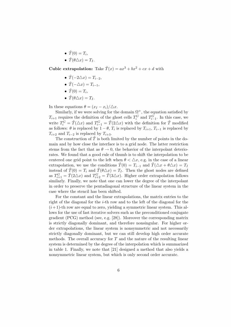
Figure 3: Solution of the Laplace equation on an irregular domain in twospatial dimensions. The exact solution is T = sin(πx)+ sin(πy)+ cos(πx)+cos(πy) + x6 + y6 in Ω−. The grid size is 64 × 64, and the ghost cells aredefined using cubic extrapolation.

23

101

102

103

10−9

10−8

10−7

10−6

10−5

10−4

10−3

10−2

10−1

100

Figure 4: Error analysis in the L∞-norm for the two dimensional Laplaceequation. The open symbols represent the errors versus the number of gridnodes on a loglog scale, and the solid lines are the least square fits with slopes-.85, -1.94, -2.94 and -3.96 in the case where the ghost cells are defined byconstant, linear, quadratic and cubic extrapolation, respectively. Note thaton a 32 × 32 mesh, the error for the quadratic extrapolation is the sameas that for the cubic extrapolation. This is an example where there wasnot enough points within the domain to construct a cubic interpolant andthe algorithm is temporarily forced to use a quadratic interpolant. More-over, this is exacerbated by our use of the L∞-norm. The L1 error is moreforgiving, since it is based on averaging.

24

101

102

103

10−11

10−10

10−9

10−8

10−7

10−6

10−5

Figure 5: Error analysis in the L∞-norm for the one dimensional heat equa-tion. The open symbols represent the error versus the number of grid nodeson a loglog scale, and the solid line depicts the least square fit with slope-4.14 in the case where the ghost cells are defined by cubic extrapolation.

25

−1 −0.8 −0.6 −0.4 −0.2 0 0.2 0.4 0.6 0.8 1−1

0

1

−0.6

−0.4

−0.2

0

0.2

0.4

0.6

0.8

1

1.2

Figure 6: Solution of the heat equation on an irregular domain in two spatialdimensions. The exact solution is T = e−2t sin(x) sin(y) in Ω−. The gridsize is 64× 64, and the ghost cells are defined by cubic extrapolation.

26

101

102

103

10−9

10−8

10−7

10−6

10−5

10−4

Figure 7: Error analysis in the L∞-norm for the two dimensional heat equa-tion. The open symbols represent the error versus the number of grid nodeson a loglog scale, and the solid line depicts the least square fit with slope-3.94 in the case where the ghost cells are defined by cubic extrapolation.

27

−Ω

Ω+

?

Interface at time n+1Interface at time n

Figure 8: Interface at time tn (dashed line) and tn+1 (solid line). The darkpoint with a question mark represents a grid node that is swept over by theinterface between two consecutive time steps, and where a valid value of Tn

needs to be extrapolated in a non-Cartesian normal direction in order toevaluate fn = Tn + 4t

2 An(4)Tn in equation (7).

28

10 20 30 40 50 60 70 80 90 100

10

20

30

40

50

60

70

80

90

100

10 20 30 40 50 60 70 80 90 100

10

20

30

40

50

60

70

80

90

100

Figure 9: Top: Plots of several isocontours of the solution extrapolated in thenormal direction from inside the disk to the outside (cubic extrapolation).Bottom: Exact solution for the sake of comparison.

29

101

102

103

10−6

10−5

10−4

10−3

10−2

10−1

100

101

Figure 10: Error analysis in the L∞-norm for the two dimensional definitionof the ghost cells defined by cubic extrapolation in the normal direction asproposed in [1]. The open symbols are the errors in the L∞-norm, and thesolid line is a least square fit with slope −4.38.

30

101

102

103

10−8

10−7

10−6

10−5

10−4

10−3

10−2

10−1

Figure 11: Error analysis on the effect of perturbing the velocity by anO(4x) (circles), O(4x2) (squares), and O(4x3) (triangles) amount in thecase of the one dimensional Stefan problem. The symbols represent thenumerical solution on a loglog scale, and the solid lines are the least squarefits with slopes -.99, -2.03 and -3.05.

31

101

102

103

10−6

10−5

10−4

10−3

10−2

Figure 12: Error analysis in the L1 (circles) and L∞ (triangles) norms forthe two dimensional reinitialization equation (10). We use a fifth orderaccurate WENO discretization in space and a third order accurate TVDRunge-Kutta discretization in time. The initial data is φ = eρ−2.313 − 1,with ρ =

√x2 + y2. The symbols represent the errors on a loglog scale, and

the solid lines are the least square fits with slopes -2.04, -1.88, respectively.

32

101

102

103

10−11

10−10

10−9

10−8

10−7

10−6

10−5

Figure 13: Error analysis in the L∞-norm for the one dimensional Stefanproblem on a loglog scale. The ghost cells are defined via cubic extrapola-tion, and we use the Crank-Nicholson scheme with 4t ≈ 4x2. The starsdepict the errors when the exact velocity is given, and the triangles illus-trate the errors when the velocity is computed. The solid lines are the leastsquare fits with slopes -4.03 and -3.10.

33

101

102

103

104

10−9

10−8

10−7

10−6

10−5

10−4

Figure 14: Error analysis in the L∞-norm for the one dimensional Frankspheres solution (the interface velocity is not constant in time). The ghostcells are defined by cubic extrapolation, and we use the Crank-Nicholsonscheme with 4t ≈ 4x3/2. The symbols represent the numerical solution ona loglog scale, and the solid line is the least square fit with slope -2.18.

34

101

102

103

10−10

10−9

10−8

10−7

10−6

10−5

Figure 15: Error analysis in the L∞-norm for the one dimensional Frankspheres solution (the interface velocity is not constant in time). The ghostcells are defined via cubic extrapolation, and we use the Crank-Nicholsonscheme with 4t ≈ 4x3/2. The time discretization involves iterating on thevelocity as described in section 4.3. The symbols represent the numericalsolution on a loglog scale, and the solid line is the least square fit with slope-3.02.

35

−1 −0.8 −0.6 −0.4 −0.2 0 0.2 0.4 0.6 0.8 1−1

−0.8

−0.6

−0.4

−0.2

0

0.2

0.4

0.6

0.8

1

Figure 16: Interface evolution in the case of the two dimensional Frankspheres solution.

−1 −0.8 −0.6 −0.4 −0.2 0 0.2 0.4 0.6 0.8 1−0.12

−0.1

−0.08

−0.06

−0.04

−0.02

0

−1 −0.8 −0.6 −0.4 −0.2 0 0.2 0.4 0.6 0.8 1

−0.06

−0.05

−0.04

−0.03

−0.02

−0.01

0

Figure 17: Cross section of the two dimensional Frank spheres solution attinitial = 1 (left) and tfinal = 2.89 (right).

36

101

102

103

10−8

10−7

10−6

10−5

10−4

10−3

10−2

Figure 18: Error analysis in the L∞-norm for the two dimensional Frankspheres solution. The triangles illustrate the accuracy obtained with thescheme presented in [9], and the circles represent the accuracy obtainedwith the algorithm presented in section 4. The open symbols are the errorsin the maximum norm, and the solid lines are least square fits with slopes-.80 and -3.07, respectively.

37

References

[1] Aslam, T., A Partial Differrential Equation Approach to Multidimen-sional Extrapolation, J. Comput. Phys. 193, 349-355 (2003).

[2] Chen, S., Merriman, B., Osher, S. and Smereka, P., A Simple LevelSet Method for Solving Stefan Problems, J. Comput. Phys. 135, 8-29(1997).

[3] Chopp, D., Some Improvement of the Fast Marching Method, SIAM J.Sci. Comput. 23, 230-244 (2001).

[4] Chong, T., A Variable Mesh Finite difference Method for Solving aClass of Parabolic Differential Equations in one Space Variable, SIAMJ. Num. Anal. 15, 835-857 (1978).

[5] Chorin, A., Curvature and Solidification, J. Comput. Phys. 58, 472-490(1985).

[6] Fedkiw, R., Aslam, T., Merriman, B., and Osher, S., A Non-OscillatoryEulerian Approach to Interfaces in Multimaterial Flows (The GhostFluid Method), J. Comput. Phys. 152, 457-492 (1999).

[7] George, W. and Warren, J., A Parallel 3D Dendritic Growth SimulatorUsing the Phase-Field Method, J. Comput. Phys. 177, 264-283 (2002).

[8] Gibou, F., Fedkiw, R., Caflisch, R. and Osher, S., A Level Set Approachfor the Simulation of Dendritic Growth, J. Sci. Comput. 19, 183-199(2003).

[9] Gibou, F., Fedkiw, R., Cheng, L-T. and Kang, M., A Second OrderAccurate Symmetric Discretization of the Poisson Equation on IrregularDomains, J. Comput. Phys. 176, 1-23 (2002).

[10] Kim, Y.-T., Goldenfeld, N. and Dantzig, J., Computation of DendriticMicrostructures using a Level Set Method, Phys. Rev. E 62, 2471-2474(2000).

[11] Hoffman, J., Relationship Between the Truncation Errors of CenteredFinite-Difference Approximations on Uniform and Nonuniform Meshes,J. Comput. Phys. 46, 469-474 (1982).

[12] Jiang, G.-S. and Peng, D., Weighted ENO Schemes for Hamilton JacobiEquations, SIAM J. Sci. Comput. 21, 2126-2143 (2000).

38

[13] Jiang, G.-S. and Shu, C.-W., Efficient Implementation of WeightedENO Schemes, J. Comput. Phys. 126, 202-228 (1996).

[14] Johansen, H., Cartesian Grid Embedded Boundary Finite DifferenceMethods for Elliptic and Parabolic Differential Equations on IrregularDomains, Ph.D. Thesis, University of California, Berkeley, CA 1997.

[15] Johansen, H. and Colella, P., A Cartesian Grid Embedded BoundaryMethod for Poisson’s Equation on Irregular Domains, J. Comput. Phys.147, 60-85 (1998).

[16] Juric, D. and Tryggvason, G., A Front Tracking Method for DendriticSolidification, J. Comput. Phys. 123, 127-148 (1996).

[17] Karma, A. and Rappel, W.-J., Quantitative Phase-Field Modeling ofDendritic Growth in Two and Three Dimensions, Phys. Rev. E 57,4323-4349 (1997).

[18] Kim, Y.-T., Goldenfeld, N. and Dantzig, J., Computation of DendriticMicrostructures using a Level Set Method, Phys. Rev. E 62, 2471-2474(2000).

[19] Kreiss, H.-O., Manteuffel, T., Swartz, B., Wendroff, B. and White, A.,Supra-Convergent Schemes on Irregular Grids Math. Comp. 47, 176,537-554 (1986).

[20] Lambert, J., Numerical Methods for Ordinary Differential Systems, Wi-ley & Sons, New York, 1993.

[21] LeVeque, R. and Li, Z., The Immersed Interface Method for EllipticEquations with Discontinuous Coefficients and Singular Sources, SIAMJ. Num. Anal. 31, 1019-1044 (1994).

[22] Liu, X-D., Osher, S., and Chan, T., Weighted Essentially Non-Oscillatory Schemes, J. Comput. Phys. 126, 200-212 (1996).

[23] Manteuffel, T. and White, A., The Numerical Solution of Second-OrderBoundary Value Problems on Nonuniform Meshes, Math. Comp. 47,176, 511-535 (1986).

[24] Osher, S. and Fedkiw, R., Level Set Methods and Dynamic ImplicitSurfaces, Springer-Verlag, New York (2002).

[25] Peskin, C., Flow Patterns Around Heart Valves: A Numerical Method,J. Comput. Phys. 10, 252-271 (1972).

39

[26] Plapp, M. and Karma, A., Multiscale Finite-Difference-Diffusion-Monte-Carlo Method for Simulating Dendritic Solidification, J. Com-put. Phys. 165, 592-619 (2000).

[27] Schmidt, A., Computation of Three Dimensional Dendrites with FiniteElements, J. Comput. Phys. 125, 293-312 (1996).

[28] Saad, Y., Iterative Methods for Sparse Linear Systems, PWS publishingcompany, Boston (1996).

[29] Sethian, J., A Fast Marching Level Set Method for Monotonically Ad-vancing Fronts, Proc. Nat. Acad. Sci. 93, 1591-1595 (1996).

[30] Sethian, J., Level Set Methods and Fast Marching Methods, CambridgeUniversity Press, Cambridge, (1999).

[31] Sethian, J. and Strain, J., Crystal Growth and Dendritic Solidification,J. Comput. Phys. 98, 231-253 (1992).

[32] Sussman, M. and Hussaini, M.Y., A Discontinuous Spectral ElementMethod for the Level Set Equation, J. Sci. Comput. 19, 479-500 (2003).

[33] Sussman, M., Smereka, P. and Osher, S., A Level Set Approach forComputing Solutions to Incompressible Two-Phase Flow, J. Comput.Phys. 114, 146-159 (1994).

[34] Tsitsiklis, J., Efficient algorithms for Globally Optimal Trajectories,IEEE Trans. on Automatic Control 40, 1528-1538 (1995).

[35] Udaykumar, H., Mittal, R. and Shyy, W., Computation of Solid-LiquidPhase Fronts in the Sharp Interface Limit on Fixed Grids, J. Comput.Phys. 153, 535-574 (1999).

[36] Zhao, P. and Heinrich, J., Front Tracking Finite Element Method forDendritic Solidification, J. Comput. Phys. 173, 765-796 (2001).

40