A Formal and Empirical Analysis of the Fuzzy Gamma

Rank Correlation Coefficient

Maria Dolores Ruiza, Eyke Hullermeierb

a Department of Computer Science and Artificial IntelligenceUniversity of Granada, Spain

bDepartment of Mathematics and Computer ScienceMarburg University, Germany

Abstract

The so-called gamma coefficient is a well-known rank correlation measure

frequently used to quantify the strength of dependence between two variables

with ordered domains. To increase the robustness of this measure toward

noise in the data, a generalization of the gamma coefficient has recently been

developed on the basis of fuzzy order relations. The goal of this paper is

threefold. First, we analyze some formal properties of the fuzzy gamma

coefficient. Second, we complement the original experiments, which have

been conducted on a simple artificial data set, by a more extensive empirical

evaluation using real-world data. On the basis of these empirical results, we

provide some basic insights and offer an explanation for the effectiveness of

the fuzzy gamma coefficient. Third, we propose an alternative motivation

for the measure, based on the idea of (fuzzy) equivalence relations induced

by limited precision in the perception of measurements.

Keywords: rank correlation, gamma rank correlation measure, fuzzy order

relations, fuzzy rank correlation, noisy data, equivalence relations

Preprint submitted to Information Sciences January 5, 2012

1. Introduction

Rank correlation measures have been studied extensively in non-parametric

statistics and are routinely used in diverse fields of application, including clus-

tering [3], information retrieval [15, 18], data mining [9, 16], economics [1, 17],

and image processing [4, 2]. In contrast to numerical correlation measures

such as the Pearson correlation, rank correlation measures are only based on

the ordering of the observed values of a variable. Thus, measures of this kind

are more widely applicable, not only to numerical but also to non-numerical

variables with an ordered domain (i.e., measured on an ordinal scale).

Roughly speaking, when deriving a rank correlation, each value is first

replaced by its rank, and the correlation is then computed on the rank data

thus obtained. Mapping numerical values to their ranks does of course pro-

duce a certain loss of information. In many cases, this is intended and makes

perfect sense, for example if a numerical variable does not have a natural (or

unique) scale of measurement1 or may contain outliers that would strongly

bias a numerical correlation measure. On the other hand, a very small dif-

ference between two values may no longer be distinguished from a very large

difference, since both could be mapped to adjacent ranks and, therefore, have

an equal (transformed) distance of 1. Moreover, the robustness toward out-

liers, i.e., extremely small or large values, comes at the price of a certain

sensitivity toward small changes: In many cases, a small increase or decrease

of a value will not have any effect at all, but in some cases it may induce

1Note, for example, that a non-numerical transformation (like a log-transformation) of

one variable will change its correlation with another variable.

2

a swapping of adjacent ranks. Thus, a small change between the numeri-

cal values can be “boosted” to a distance of 1 between the associated rank

values. Obviously, this property is especially undesirable in the presence of

noise in the data.

To overcome problems of this kind, Bodenhofer and Klawonn [8] have

recently proposed a fuzzy variant of a rank correlation measure known as

Goodman and Kruskal’s gamma measure [12]. Roughly speaking, the use of

fuzzy order relations allows the authors to distinguish between negligible and

significant differences between numerical values in a more subtle way, and to

decrease the influence of the former. Thus, the rank correlation measure

becomes arguably more robust toward noise.

The goal of this paper is threefold. First, we analyze some formal prop-

erties of the fuzzy rank correlation measure proposed by Bodenhofer and

Klawonn. Second, we complement the authors’ experiments, which have

been conducted on a simple artificial data set, by a more extensive empirical

evaluation using real-world data. On the basis of these empirical results, we

provide some basic insights and offer an explanation for the effectiveness of

the fuzzy gamma coefficient.

Third, we offer an alternative motivation of the measure, based on the

idea of equivalence relations induced by limited precision in the perception

of measurements. As an illustrating example, suppose we are interested in

the correlation, if any, between the length of a submitted manuscript and the

recommendation of the reviewer. Since the recommendation is taken from an

ordinal scale (e.g., accept, minor revision, major revision, reject), only a rank

correlation measure can be computed. As will be explained in more detail

3

later on, such measures are mainly based on the order relation between two

measurements. In the case of the recommendation scale, this order relation

is simply defined by the ordinal scale; for example, accept > minor revision.

As for the length of a manuscript, one may simply compare two papers in

terms of the respective number of words. This approach, however, is unlikely

to capture the reviewer’s perception. For example, a reviewer will normally

not perceive an article A as longer than an article B, only because the former

has one or two words more than the latter. In this situation, a fuzzy order

relation (on the word count of manuscripts) can be used in a quite reasonable

way, namely for expressing that an article A can be longer than B “to some

degree”. In other words, it allows for modeling the “perceived difference in

length” between two articles as a gradual relation, which is arguably more

natural than treating it in a binary way.

The above example does also hint at another appealing property of fuzzy

rank correlation, namely the fact that they combine properties of both, nu-

merical and rank correlation. Thus, like in the example, it becomes possible

to compare variables that are measured on scales of different types. In the re-

mainder of the paper, we shall mainly focus on the case where both variables

are numeric, mainly because this case was also studied by Bodenhofer and

Klawonn. One should keep in mind, however, that the approach is in prin-

ciple more general and only requires the possibility to equip a domain with

a reasonable fuzzy equivalence relation (note that the canonical > relation

determined by an ordinal scale can be seen as a degenerate fuzzy relation).

The remainder of the paper is organized as follows. In the next section,

we recall the essential background for understanding the rest of the paper,

4

including rank correlation measures, fuzzy order relations, and the fuzzy ex-

tension of the gamma coefficient originally introduced in [8]. In Section 3, we

derive some results throwing light on formal properties of the fuzzy gamma.

In Section 4, we elaborate on the idea of using the fuzzy gamma as a noise-

tolerant version of the original gamma coefficient. An alternative interpreta-

tion of the fuzzy gamma in terms of a “perception-based” rank correlation

measure masking inappropriate precision in the measurement of quantities is

then proposed and investigated in Section 5. Finally, we conclude the paper

with a couple of remarks and an outlook on future work in Section 6.

2. Rank Correlation Coefficients

In this section, we give a brief overview of rank correlation measures in

general and then focus on the gamma coefficient. We start with some formal

definitions which are important to understand the rest of the paper. We also

address the use of rank correlation coefficients as distance measures.

2.1. Basic Correlation Measures

A rank correlation measure is applied to n ≥ 2 paired observations

{ (xi, yi) }ni=1 ⊂ (X× Y)n (1)

of a pair of variables (X, Y ), where X and Y are two linearly ordered do-

mains (e.g., subsets of the reals); we denote x = (x1, x2, . . . , xn) and y =

(y1, y2, . . . , yn). The goal is to measure the dependence between the two vari-

ables in terms of their tendency to increase and decrease in the same or the

opposite direction. If an increase in X tends to come along with an increase

5

in Y , then the (rank) correlation is positive. The other way around, the cor-

relation is negative if an increase in X tends to come along with a decrease

in Y . If there is no dependency of either kind, the correlation is (close to) 0.

Among the best-known and most frequently used measures are Spear-

man’s rank correlation coefficient (Spearman’s rho for short), Kendall’s tau

and Goodman and Kruskal’s gamma. Spearman’s rho is given by the sum of

squared rank distances, normalized to the range [−1, 1]:

ρ = 1− 6∑n

i=1(r(xi)− r(yi))2

n(n2 − 1), (2)

where r(xi) = #{j ∈ {1, . . . , n} |xj ≤ xi} is the rank of value xi in the set of

observations {x1, . . . , xn}. Here, we assume that the data does not contain

any ties, i.e., xi 6= xj for 1 ≤ i 6= j ≤ n. In the presence of ties, a proper

generalization of (2) can be used.

Kendall’s tau coefficient is defined in terms of the number of concordant,

discordant, and tied data points. For a given index pair (i, j) ∈ {1, . . . , n}2,

we say that (i, j) is concordant if xi < xj and yi < yj or xi > xj and yi > yj;

it is discordant if xi < xj and yi > yj or xi > xj and yi < yj; it is a tie if

either xi = xj or yi = yj. Denoting

C = #{(i, j) | i < j, xi < xj and yi < yj or xi > xj and yi > yj},

D = #{(i, j) | i < j, xi < xj and yi > yj or xi > xj and yi < yj},

T = #{(i, j) | i < j, xi = xj or yi = yj},

(3)

the original Kendall tau is defined as

τa =C −D

12n(n− 1)

. (4)

When there are no ties (T = 0) and the two rankings coincide, we have 12n(n−

1) concordant pairs and no discordant pair, so τa = 1; if one ranking is the

6

reverse of the other one, we have τa = −1. In the presence of ties, however,

this measure does not assume the extreme values −1 and +1 and, hence, is

not well normalized. Like in the case of Spearman’s rho, a generalization can

be defined by properly adapting the normalizing constant in (4).

Another quite simple measure is Goodman and Kruskal’s gamma rank

correlation [12], which simply ignores all ties. It is defined as

γ =C −DC +D

(5)

and coincides with Kendall’s tau when there are no ties in the data. Through-

out the remainder of the paper, we shall focus on the measure (5).

2.2. Fuzzy Equivalence and Order Relations

Bodenhofer and Klawonn [8] advocate the use of the gamma coefficient as

a reasonable correlation measure but also indicate problems in the presence

of noise in the data. To make it more robust toward noisy data, they propose

a fuzzy generalization which is based on concepts of fuzzy orderings and >-

equivalence relations, where > denotes a triangular norm (t-norm) [6, 8]. We

assume that the reader is familiar with the basic concepts of triangular norms

and fuzzy relations [6]. Yet, to make the paper more self-contained, we briefly

recall some basic definitions which are necessary for the understanding of the

rest of the paper.

Definition 1. A fuzzy relation E : X×X→ [0, 1] is called fuzzy equivalence

with respect to a t-norm>, for brevity>-equivalence, if and only if it satisfies

the following three axioms: For all x, y, z ∈ X,

(i) reflexivity: E(x, x) = 1,

7

(ii) symmetry: E(x, y) = E(y, x),

(iii) >-transitivity: >(E(x, y), E(y, z)) ≤ E(x, z).

Definition 2. A fuzzy relation L : X × X → [0, 1] is called fuzzy ordering

with respect to a t-norm > and a >-equivalence E : X × X → [0, 1], for

brevity >-E-ordering, if and only if it satisfies the following three axioms:

For all x, y, z ∈ X,

(i) E-reflexivity: E(x, y) ≤ L(x, y),

(ii) >-E-antisymmetry: >(L(x, y), L(y, x)) ≤ E(x, y),

(iii) >-transitivity: >(L(x, y), L(y, z)) ≤ L(x, z).

Moreover, we call a>-E-ordering L strongly complete if max(L(x, y), L(y, x)) =

1 for all x, y ∈ X. Considering the special cases of the well-known and fre-

quently used Lukasiewicz t-norm >L and the product t-norm >P , defined

by

>L(x, y) = max(0, x+ y − 1),

>P (x, y) = xy,

it can be verified that

Er(x, y) = max

(0, 1− 1

r|x− y|

)E ′r(x, y) = exp

(−1

r|x− y|

) (6)

are >-equivalences on R associated with >L and >P , respectively, where

r > 0. The following theorem proved in [5] gives a full characterization of

strongly complete orderings.

8

Theorem 1. (Bodenhofer [5]). Let L be a binary fuzzy relation on X and let

E be a>-equivalence on X. Then the following two statements are equivalent:

(i) L is a strongly complete >-E-ordering on X.

(ii) There exists a linear ordering � such that relation E is compatible2

with � and, moreover, L can be represented as follows:

L(x, y) =

1 if x � y

E(x, y) otherwise(7)

This theorem implies that

Lr(x, y) = min

{1,max

(0, 1− 1

r(x− y)

)}is a strongly complete >L-Er-ordering on R, and

L′r(x, y) = min

{1, exp

(−1

r(x− y)

)}is a strongly complete >P -E ′r-ordering on R.

Definition 3. A binary fuzzy relation R is called a strict fuzzy ordering

with respect to a t-norm > and a >-equivalence E, or strict >-E-ordering

for short, if R is irreflexive (R(x, x) = 0 for all x ∈ X), >-transitive and

E-extensional, which means that

>(E(x, x′), E(y, y′), R(x, y)) ≤ R(x′, y′)

for all x, x′, y, y′ ∈ X [7].

2A fuzzy relation E is compatible with an order relation � on X if and only if E(x, z) ≤

min{E(x, y), E(y, z)} holds for all x � y � z.

9

As argued in [7], the most appropriate way of extracting a strict fuzzy

ordering R from a >-E-ordering L is to define

R(x, y) = min{L(x, y), N(L(y, x))} , (8)

where N(x) = sup{y ∈ [0, 1] | >(x, y) = 0} is the residual negation of >.

Examples of this construction are the relations

Rr(x, y) = min

{1,max

{0,

1

r(y − x)

}},

R′r(x, y) = max

{0, 1− exp

(−1

r(y − x)

)}.

For a strongly complete>L-E-ordering L, the relation (8) is given byR(x, y) =

1−L(y, x); moreover, R(x, y)+E(x, y)+R(y, x) = 1 and min{R(x, y), R(y, x)} =

0.

2.3. A Fuzzy Extension of the Gamma Rank Correlation

Consider a set of paired data points (1) and assume to be given two >L-

equivalences EX : X2 → [0, 1] and EY : Y2 → [0, 1], a strongly complete >L-

EX-ordering LX : X2 → [0, 1] and a strongly complete >L-EY-ordering LY :

Y2 → [0, 1]. We can then define a strict>L-EX-ordering on X by RX(x1, x2) =

1−LX(x2, x1) and a strict>L-EY-ordering on Y by RY(y1, y2) = 1−LY(y2, y1).

Using these relations, the concepts of concordance and discordance of data

points can be generalized as follows: Given an index pair (i, j), the degree to

which this pair is concordant, discordant, and tied is defined, respectively, as

C(i, j) = >(RX(xi, xj), RY(yi, yj)), (9)

D(i, j) = >(RX(xi, xj), RY(yj, yi)), (10)

T (i, j) = ⊥(EX(xi, xj), EY(yi, yj)), (11)

10

where > is a t-norm and ⊥ is the dual t-conorm of > (i.e. ⊥(x, y) = 1 −

>(1− x, 1− y)). The following equality holds for all index pairs (i, j):

C(i, j) + C(j, i) + D(i, j) + D(j, i) + T (i, j) = 1.

Adopting the simple sigma-count principle to measure the cardinality of a

fuzzy set [10], the number of concordant and discordant pairs can be com-

puted, respectively, as

C =n∑

i=1

∑j 6=i

C(i, j), D =n∑

i=1

∑j 6=i

D(i, j).

The fuzzy ordering-based gamma rank correlation measure γ, or simply fuzzy

gamma, is then defined as

γ =C − DC + D

. (12)

Note that this measure is “parameterized” by the underlying fuzzy orderings,

i.e., a t-norm > and fuzzy equivalence relations EX and EY.

From the definition of γ, it is clear that the basic idea is to decrease the

influence of “close-to-tie” pairs (xi, yi) and (xj, yj). Roughly speaking, such

pairs, whether concordant or discordant, are turned into a partial tie, and

hence are ignored to some extent. Or, stated differently, there is a smooth

transition between being concordant (discordant) and being tied. The larger

the scaling parameter r, the more a pair is considered as a partial tie; see

Fig. 1 for an illustration of the difference between the crisp and the fuzzy

case.

As a side remark, we note that a fuzzy equivalence relation E may have

a probabilistic interpretation, although this is not required by the formal

framework. Consider, for example, the case of numerical data corrupted with

11

difference between x−values

diffe

rence b

etw

eeny−

valu

es

discordance

discordanceconcordance

concordance

ties

difference between x−values

diffe

rence b

etw

eeny−

valu

es

discordance

discordanceconcordance

concordance

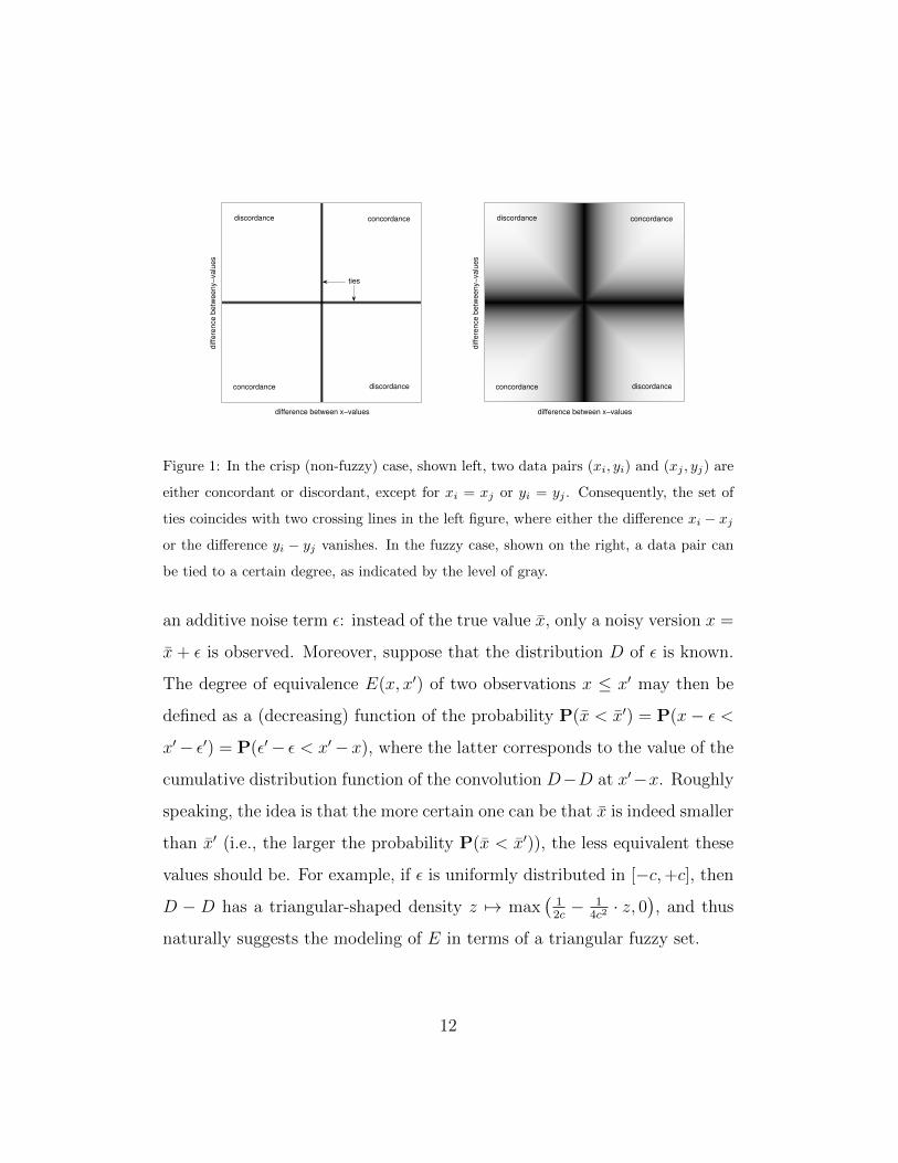
Figure 1: In the crisp (non-fuzzy) case, shown left, two data pairs (xi, yi) and (xj , yj) are

either concordant or discordant, except for xi = xj or yi = yj . Consequently, the set of

ties coincides with two crossing lines in the left figure, where either the difference xi − xjor the difference yi − yj vanishes. In the fuzzy case, shown on the right, a data pair can

be tied to a certain degree, as indicated by the level of gray.

an additive noise term ε: instead of the true value x, only a noisy version x =

x + ε is observed. Moreover, suppose that the distribution D of ε is known.

The degree of equivalence E(x, x′) of two observations x ≤ x′ may then be

defined as a (decreasing) function of the probability P(x < x′) = P(x− ε <

x′− ε′) = P(ε′− ε < x′− x), where the latter corresponds to the value of the

cumulative distribution function of the convolution D−D at x′−x. Roughly

speaking, the idea is that the more certain one can be that x is indeed smaller

than x′ (i.e., the larger the probability P(x < x′)), the less equivalent these

values should be. For example, if ε is uniformly distributed in [−c,+c], then

D − D has a triangular-shaped density z 7→ max(

12c− 1

4c2· z, 0

), and thus

naturally suggests the modeling of E in terms of a triangular fuzzy set.

12

3. Formal Properties of Gamma and Fuzzy Gamma

3.1. Metric Properties

Consider a set X endowed with a total order; without loss of generality,

we can assume that X is a subset of the reals. Ideally, a rank correlation

measure C should satisfy the following for all n ∈ N and x,y ∈ Xn:

C1: −1 ≤ C(x,y) ≤ 1

C2: C(x,y) = C(y,x)

C3: C(x,y) = 1 if the elements in x are in the same order as those in y,

i.e., r(x) = r(y); in particular, C(x,x) = 1.

It is quite easy to see that γ satisfies all of these properties. Note that

property C3 is fulfilled by all measures that only depend on the ranks r(x) =

(r(x1), r(x2) . . . r(xn)) and r(y) = (r(y1), r(y2) . . . r(yn)). This property is

intentionally violated by the fuzzy variant γ.

The above properties may remind one of related properties of distance

measures, and indeed, some rank correlation measures are in fact normalized

versions of corresponding distance measures. For example, Spearman’s rho is

an affine transformation of the sum of squared rank distances to the interval

[−1,+1], and Kendall’s tau is a similar transformation of the Kendall dis-

tance, namely the sum of rank inversions [13]. To study the rank correlation

measures γ and γ from the perspective of a distance measure, recall the basic

definition of a metric:

Definition 4. A mapping d : A × A → R is a metric on A if and only if it

fulfills the following for all a, b, c ∈ A:

– d(a, b) ≥ 0 (non-negativity),

13

– d(a, b) = 0 ⇔ a = b (separation),

– d(a, b) = d(b, a) (symmetry),

– d(a, c) ≤ d(a, b) + d(b, c) (triangle inequality).

Let x,y ∈ Xn. The measure

d(x,y) = 1− γ(x,y) = 1− C −DC +D

=2D

C +D

is obviously non-negative (since −1 ≤ γ ≤ 1) and symmetric (since γ is also

symmetric). The separation property cannot be satisfied, as a rank corre-

lation measure depends on the concrete values (xi, yi) ∈ X2 only indirectly

via the corresponding ranks. It holds, however, that d(x,y) = 0 implies

r(x) = r(y).

It is also easy to see that the triangle inequality does not hold for d. Here is

a simple counterexample: With x = (1, 2, 3), y = (1, 1, 2) and z = (2, 1, 2),

we have γ(x,y) = 1, γ(x, z) = 0, γ(y, z) = 1, and hence 1 = d(x, z) 6≤

d(x, z) + d(z,y) = 0. As a main reason for the violation of this inequality,

note that, due to the ignorance of ties, the pairwise distance computations

may refer to completely different elements. For example, since y1 and y2 are

tied, γ(x,y) is completely determined by the comparison of the index pairs

(1, 3) and (2, 3). Likewise, since z1 and z3 are tied, γ(y, z) only depends

on the index pair (2, 3), while γ(x, z) depends on the index pairs (1, 2) and

(2, 3).

Replacing γ by the fuzzy version γ, we obtain

d(x,y) = 1− γ(x,y) = 1− C − DC + D

=2D

C + D.

Again, it is obvious that d(x,y) ≥ 0 (because −1 ≤ γ(x,y) ≤ 1) and

that symmetry holds (symmetry of a t-norm implies symmetry of C and D).

14

Moreover, when comparing x with itself, the degree of discordance of the

index pair (i, j) is

>(RX(xi, xj), RX(xj, xi)) ≤ RX(xi, xi)

= 1− LX(xi, xi)

= 1−

1 if xi ≤ xi

E(xi, xi) otherwise

= 1− 1 = 0

where we have used the >-transitivity of RX, Theorem 1 and the reflexivity of

E. (Note that, in particular, L can be written as L(x, y) = min(1, E(x, y)),

as can be seen for the cases of Lukasiewicz and product t-norms). Therefore,

the total degree of discordance is 0, which means that reflexivity also holds.

Like in the non-fuzzy case, the triangle inequality does of course not hold.

To show this, the same counterexample as above can be used. In fact, with

x = (1, 2, 3), y = (1, 1, 2), z = (2, 1, 2), γ(x,y) is nearly zero while γ(x, z)

and γ(y, z) are close to 1 if 0 < r < 1, both for the Lukasiewicz and the

product t-norm.

In summary, it can be seen that γ satisfies desirable properties of a rank

correlation measure, though not all properties of a metric (especially not

the triangle inequality). More importantly, however, none of the properties

satisfied by γ are lost when passing to the fuzzy version γ except, of course,

property C3.

15

3.2. Limit Behavior of the Fuzzy Gamma

The concrete values produced by the γ measure depend on the scaling

parameter r. In the following, we study the influence of r on the relation

between γ and γ for the cases of the product and the Lukasiewicz t-norm.

More specifically, we show that the natural requirement of recovering the

original γ for the case r = 0 is indeed satisfied. More formally: γ converges

to γ as r → 0.

Proposition 1. Let γ, γL and γP be defined as in the previous section. The

following properties are satisfied:

i. limr→0

γL = γ

ii. limr→0

γP = γ

Proof. i. We first compute some simpler limits:

• If xj − xi < 0 then limr→0

1− 1

r(xj − xi) =∞, so lim

r→0LX(xj, xi) = 1.

• If xj − xi > 0 then limr→0

1− 1

r(xj − xi) = −∞, so lim

r→0LX(xj, xi) = 0.

• If xj − xi = 0 then we have a tie.

We distinguish four cases when taking the limit r → 0:

(a) If xj−xi < 0 and yj−yi < 0, then limr→0

LX(xj, xi) = 1 and limr→0

LY(yj, yi) =

1, therefore limr→0

C(i, j) = 0.

(b) If xj−xi < 0 and yj−yi > 0, then limr→0

LX(xj, xi) = 1 and limr→0

LY(yj, yi) =

0, therefore limr→0

C(i, j) = 0.

(c) If xj−xi > 0 and yj−yi < 0, then limr→0

LX(xj, xi) = 0 and limr→0

LY(yj, yi) =

1, therefore limr→0

C(i, j) = 0.

16

(d) If xj−xi > 0 and yj−yi > 0, then limr→0

LX(xj, xi) = 0 and limr→0

LY(yj, yi) =

0, therefore limr→0

C(i, j) = 1.

Changing the index j by i in the previous reasoning for computing limr→0

C(j, i),

we conclude that if xj − xi < 0 and yj − yi < 0, then limr→0

C(j, i) = 1 and 0

in the rest of the cases. Analogously, for D, we have that limr→0

D(i, j) = 1 if

xj−xi > 0 and yj−yi < 0 and 0 otherwise, and limr→0

D(j, i) = 1 if xj−xi < 0

and yj − yi > 0, and 0 in the rest of the cases. We end the proof by noting

that

limr→0

n∑i=1

n∑j 6=i

C(i, j) =n∑

i=1

n∑j 6=i

limr→0

C(i, j) = C

limr→0

n∑i=1

n∑j 6=i

D(i, j) =n∑

i=1

n∑j 6=i

limr→0

D(i, j) = D.

ii. The proof is analogous to the previous one.

In principle, one may of course also look for the limits of γ when r →

∞. First, however, note that this case is hardly relevant from a practical

point of view, as it means that all values are considered as completely tied.

Theoretically, this case causes problems, too, since the limit does often not

even exist. For example, when using Er as an equivalence relation, it is

easy to verify that T (i, j) = 1 for all i, j and hence C = D = 0 as soon

as r > 2 maxi {|xi − xi|, |yi − yj|}, which means that the numerator and the

denominator in (12) is 0 and the term no longer well-defined.

There are, however, special cases in which the limit does indeed exist.

Bodenhofer and Klawonn [8] point out that, in principle, the t-norm in (9–

10) does not necessarily need to coincide with the t-norm underlying the

17

definition of the fuzzy order relations. For example, taking > = min (and

Er as before), it can be seen that, for sufficiently large r, the degree of

concordance (discordance) of each concordant (discordant) pair (xi, yi) and

(xj, yj) is given by r−1 · min{|xi − xj|, |yi − yj|}. Thus, the parameter r in

(12) cancels out, and the fuzzy gamma converges to

γ =

∑i<j(c(i, j)− d(i, j)) ·mij∑i<j(c(i, j) + d(i, j)) ·mij

, (13)

where mij = min{|xi − xj|, |yi − yj|}, c(i, j) = 1 if (xi, yi) and (xj, yj) are

concordant (and c(i, j) = 0 if not), and d(i, j) = 1 if (xi, yi) and (xj, yj)

are discordant (and d(i, j) = 0 if not). In other words, γ can be seen as a

modification of the standard γ, in which the influence of each pair (xi, yi)

and (xj, yj) is weighted by mij.

Despite the existence of the limit, (13) should be considered with caution,

since the measure arguably loses its original character: Instead of considering

closely neighbored data points as being tied to some degree, the idea of a tie

loses its local property. Instead, the degree of concordance (discordance), and

hence the degree of equivalence, are simply proportional to the dissimilarity of

data points (as measured by the mij). Consequently, (13) is more numerical

than rank-based (the concrete values xi and yi may have a strong influence)

and partly loses its robustness properties. For example, consider a data set

with observations (x1, y1), . . . , (xn+1, yn+1), where (xi, yi) = (i, i) for i ≤ n

and (xn+1, yn+1) = (M,−M) for some M > n + 1. Thus, while the first n

values are perfectly (linearly) correlated, the last point is an outlier. The

standard gamma is given by γ = (n2 − 3n)/(n2 + n). Thus, it is robust and

close to +1 for large n, regardless of M . In contrast, (13) strongly depends

on the value of M , and even converges to −1 for M →∞.

18

4. Fuzzy Gamma as a Robust Correlation Measure

As a main motivation for their fuzzy extension of the gamma measure, the

authors in [8] mention the goal to make the computation of rank correlation

more robust toward noise in the data. In this section, we shall analyze the

fuzzy gamma from this point of view. Thus, we assume that the observed

data {(xi, yi)}ni=1 is corrupted with noise, which means that xi = xi + εi,

where xi is a true but unknown value, and εi is an error term independent

of xi; likewise, yi = yi + ε′i. As usual, the error terms are assumed to be

independent and identically distributed.

We shall start with a kind of qualitative analysis of the effects of fuzzifying

γ. Even though this analysis is based on some simplifying assumptions, it

will help to develop a basic understanding of these effects. Moreover, it will

be corroborated later one by means of suitable experiments.

It is fair to assume that adding random noise to the true data {(xi, yi)}ni=1

will resolve some of the existing ties, if any, but not create additional ones (if

the error terms εi and ε′i are real-valued random variables with a continuous

density, then the probability to create a tie is indeed 0). So, with Ctrue, Dtrue,

and Ttrue denoting, respectively, the true number of concordant, discordant,

and tied pairs (among the (xi, yi)), and Cobs, Dobs, and Tobs, respectively,

the observed number of concordant, discordant, and tied pairs (among the

(xi, yi)), we have Tobs ≤ Ttrue or, equivalently, Cobs + Dobs ≥ Ctrue + Dtrue.

Moreover, since the distribution of error terms is typically symmetric with

mean 0, it is natural to assume that a tie will be turned into a concordant

19

and discordant pair with equal probability, which means that

Cobs ≈ Ctrue +1

2(Ttrue − Tobs) = Ctrue +

∆T

2,

Dobs ≈ Dtrue +1

2(Ttrue − Tobs) = Dtrue +

∆T

2,

where ∆T = Ttrue−Tobs ≥ 0. Regarding the computation of rank correlation,

we thus obtain

γ =Cobs −Dobs

Cobs +Dobs

=Ctrue −Dtrue

Ctrue +Dtrue + ∆T<Ctrue −Dtrue

Ctrue +Dtrue

= γtrue

if Ctrue > Dtrue and, likewise γ > γtrue if Ctrue < Dtrue. In words, a com-

putation of γ based on the observed data is biased toward 0, i.e., it will be

an underestimation of truly positive and an overestimation of truly negative

rank correlation coefficients.

Now, as mentioned previously, the basic principle underlying the fuzzy

gamma measure is to turn concordant or discordant observations into partial

ties. So, it can indeed be hoped that the “lost” ties ∆T will be recovered

to some extent and, hence, that γ will be corrected in the right direction,

namely toward the extreme values −1 or +1. Intuitively, it makes sense to

assume that C = (1 − α)Cobs, where α is the fraction of total concordance

which is turned into equality via fuzzy equivalence. Obviously, this fraction

depends on the scaling parameter r, so α = α(r). Likewise, it makes sense

to assume that D = (1− α)Dobs. In this case, however,

γ =(1− α)Cobs − (1− α)Dobs

(1− α)Cobs + (1− α)Dobs

=Cobs −Dobs

Cobs +Dobs

= γ , (14)

i.e., γ will be equal (or at least very similar) to γ. In other words, γ is

ineffective and does not correct γ toward γtrue.

20

It is important to note, however, that the above result is correct only if

the fraction α is the same for the concordant and discordant pairs. Even

though the concrete value of this quantity strongly depends on the data, it

is interesting to note that the cardinality of the concordant and discordant

pairs, respectively, is likely to have an important influence on this value. To

explain this observation, assume that Cobs > Dobs, which means that the data

is positively correlated; the case of negative correlation is treated analogously.

While the distribution of uncorrelated data is typically a cloud having the

same spatial extension in all direction, the distribution of positively corre-

lated data is normally elongated, having the shape of a kind of ellipse; see

Fig. 2 for an illustration. Now, suppose that a concordant and a discordant

pair of data are picked at random. Under the above assumption of an elon-

gated data distribution, the probability of being close to each other is higher

for the discordant than for the concordant pair (there are many concordant

pairs that are far from each other, but much less discordant pairs). This is

confirmed by the cumulative distribution functions shown in Fig. 2.

These arguments imply that, in the case of positively correlated data,

α < β, where α = α(r, Cobs) is the fraction for concordant and β = β(r,Dobs)

the fraction for discordant pairs that are turned into a tie. Consequently,

(14) becomes

γ =(1− α)Cobs − (1− β)Dobs

(1− α)Cobs + (1− β)Dobs

>Cobs −Dobs

Cobs +Dobs

= γ ,

which means that γ is indeed a proper correction of γ.

The above considerations provide evidence for the following conjectures:

• First, if the data to be analyzed is a noisy version of true data in

which ties do exist, then the fuzzy gamma may potentially be a better

21

0 0.2 0.4 0.6 0.8 10

0.2

0.4

0.6

0.8

1

0 0.5 1 1.50

0.2

0.4

0.6

0.8

1

−0.5 0 0.50

0.1

0.2

0.3

0.4

0.5

0 0.5 1 1.50

0.2

0.4

0.6

0.8

1

Figure 2: Typical examples of positively (top left) and uncorrelated (bottom left) data.

The pictures to the right show a plot of the corresponding cumulative distribution functions

mapping a distance d (x-axis) to the relative frequency of (concordant or discordant) data

pairs whose distance is at most d (y-axis). The solid line depicts this function for the

discordant data, the dashed one for the concordant data.

22

estimate than the original gamma; in this case, the performance of γ

will depend on the proper choice of the scaling parameter r.

• Second, if the original data does not contain any ties, then γ is likely

to give a biased estimate (while the original gamma is unbiased), as it

will still tend to make the estimation more extreme (i.e., closer to +1

or −1).

• Third, if the original data does not contain any ties, but the observa-

tions are noisy, then γ may potentially be a better estimate than the

original gamma; like in the first case, the performance will depend on

the proper choice of the scaling parameter r.

To explain the third conjecture, note that adding random noise to a data

set will probably make the data less correlated, and the higher the level of

noise, the stronger this effect will be (indeed, for a very high level of noise,

the original data will be completely destroyed). Therefore, computing γ on

the observed data will give a value which is probably closer to 0 than the

true rank correlation, and since γ tends to make the estimate more extreme,

it might be able to compensate for this effect.

Since the second conjecture is actually a special case of the third one

(noise level of 0), we may hypothesize that γ can be beneficial whenever the

original data is corrupted by noise, provided that the parameter r is chosen in

a proper way (specifically, the second case calls for r = 0). In the following,

we shall present some experimental studies to validate our conjectures.

23

4.1. Experiments

First evidence supporting our conjectures already comes from the exper-

iments that have been conducted in [8]. In these experiments, synthetic

data is produced by adding noise to a sample of points from the graph of

a one-dimensional function. The first function f1(·) used by the authors is

piecewise linear with a big region of ties in the middle; see Fig. 3. The second

function is parameterized and defined by y = f2(x) = x/2 + 1/4 for x ≥ 0.5

and = (1− 2q)x + q for x ≤ 0.5. This function is monotone for 0 ≤ q ≤ 0.5

and non-monotone for 0.5 ≤ q ≤ 1; again, see Fig. 3.

Comparing the performance of γ and γ as estimates of the rank correlation

(which is +1 in the first two cases and close to 0 in the third), the authors

find that γ performs extremely well in the first case, comparatively good in

the second case, but worse than γ in the third (non-monotone) case. These

results are in complete agreement with our discussion above.

0

0.2

0.4

0.6

0.8

1

0 0.2 0.4 0.6 0.8 1

0

0.2

0.4

0.6

0.8

1

0 0.2 0.4 0.6 0.8 1

0

0.2

0.4

0.6

0.8

1

0 0.2 0.4 0.6 0.8 1

Figure 3: Graphs of the functions f1(·) and f2(·) for q = 0.4 (middle) and q = 0.7 (right).

To complement these experiments on synthetic data, we resorted to the

well-known IRIS data set, a frequently used benchmark in data analysis.3

3For problems such as clustering and classification, this data set is actually not very

24

From the IRIS data, which comprises four real-valued variables and 150

observations. From the six possible two-dimensional combinations of the

four features of the data set, we choose two representative ones. The first

data set, D1, consists of the second and the fourth attribute, which are

almost uncorrelated (γ ≈ −0.16), and the second data set, D2, consists

of the third and the fourth attribute, which are highly positively corre-

lated (γ ≈ 0.84); see Fig. 4. In D1 and D2, 14% and 9% of the data

pairs are tied, respectively. We corrupted the data sets with random noise

sampled from a normal distribution with mean 0 and standard deviation

σ ∈ {0.008, 0.02, 0.04, 0.06, 0.1, 0.12, 0.15, 0.175, 0.2}. Moreover, we tried γ

with different values of the scaling parameter r ∈ {0.01, 0.06, 0.09, . . . , 0.96}.

2 2.5 3 3.5 40

0.5

1

1.5

2

2.5

0 1 2 3 4 5 6 70

0.5

1

1.5

2

2.5

Figure 4: Left: Second and fourth attribute of the IRIS data (γ ≈ −0.16). Right: Third

and fourth attribute (γ ≈ 0.84).

The results for data set D1 are shown in Fig. 5 (γ as a function of the

level of noise) and Fig. 6 (γ as a function of r). In agreement with our

expectations, γ is not able to improve the estimation of γ. On the contrary,

it tends to underestimate the true correlation, and the larger r, the stronger

challenging, which, however, is irrelevant for our purpose.

25

0 0.05 0.1 0.15 0.2

-0.2

-0.18

-0.16

-0.14

-0.12

0 0.05 0.1 0.15 0.2

-0.26

-0.24

-0.22

-0.2

-0.18

-0.16

-0.14

-0.12

0 0.05 0.1 0.15 0.2

-0.3

-0.25

-0.2

-0.15

Figure 5: Rank correlation (y-axis) as a function of the level of noise (x-axis) for data set

D1 and different values of r (left 0.01, middle 0.11, right 0.21)

.

0 0.2 0.4 0.6 0.8

-0.5

-0.45

-0.4

-0.35

-0.3

-0.25

-0.2

-0.15

0 0.2 0.4 0.6 0.8-0.5

-0.45

-0.4

-0.35

-0.3

-0.25

-0.2

-0.15

0 0.2 0.4 0.6 0.8

-0.5

-0.45

-0.4

-0.35

-0.3

-0.25

-0.2

-0.15

Figure 6: Rank correlation (y-axis) as a function of the scaling parameter r (x-axis) for

data set D1 and different levels of noise (left 0.008, middle 0.06, right 0.175).

26

this effect becomes.

0 0.05 0.1 0.15 0.2

0.675

0.7

0.725

0.75

0.775

0.8

0.825

0 0.05 0.1 0.15 0.2

0.7

0.75

0.8

0.85

0 0.05 0.1 0.15 0.2

0.7

0.75

0.8

0.85

0.9

Figure 7: Rank correlation (y-axis) as a function of the level of noise (x-axis) for data set

D2 and different values of r (left 0.01, middle 0.11, right 0.21).

0 0.2 0.4 0.6 0.8

0.8

0.85

0.9

0.95

0 0.2 0.4 0.6 0.8

0.8

0.85

0.9

0.95

0 0.2 0.4 0.6 0.8

0.75

0.8

0.85

0.9

0.95

Figure 8: Rank correlation (y-axis) as a function of the scaling parameter r (x-axis) for

data set D2 and different levels of noise (left 0.008, middle 0.06, right 0.15).

The results for data set D2 are shown in Fig. 7 and Fig. 8. This time,

the performance of γ is much better and again in agreement with what we

expect. Indeed, γ is able to improve the estimation of γ. In Fig. 8, it can

nicely be seen that there is an optimal value of r which depends on the level

of noise: The higher the noise, the larger r should be.

To validate our second and third conjecture, we need a data set without

ties. To this end, we added a very small level of random noise to the data

sets D1 and D2, respectively, and thus obtained two new data sets N1 and

N2 without ties; see Fig. 9. For these data sets, which were now taken as

the ground truth, we repeated the same experiments. The results, shown in

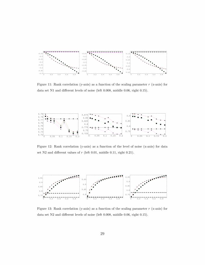
Fig. 10 and Fig. 11 for N1 and in Fig. 12 and Fig. 13 for N2, are again in

27

agreement with our conjectures. If the noise added to N1 and N2, respec-

tively, is very small, then γ tends to give estimates biased toward −1 and +1

respectively. However, when the noise becomes larger, the original γ tends

to give estimates biased toward 0, and γ compensates for this, at least for

a proper choice of r. An obvious example of this can be seen in the third

case in Fig. 13, in which γ underestimates the true correlation of N2, and

γL (γP ) repairs this for r ≈ 0.1 (r ≈ 0.05). Again, it can also be seen that

higher levels of noise require higher values of r, i.e., the choice of the optimal

r clearly depends on the level of noise.

2 2.5 3 3.5 4

0

0.5

1

1.5

2

2.5

0 1 2 3 4 5 6 7

0

0.5

1

1.5

2

2.5

Figure 9: Left: Second and fourth attribute of noise-free data set N1 (γ ≈ −0.12). Right:

Third and fourth attribute of data set N2 (γ ≈ 0.77).

0 0.05 0.1 0.15 0.2

-0.16

-0.15

-0.14

-0.13

-0.12

0 0.05 0.1 0.15 0.2-0.2

-0.18

-0.16

-0.14

-0.12

0 0.05 0.1 0.15 0.2

-0.24

-0.22

-0.2

-0.18

-0.16

-0.14

-0.12

Figure 10: Rank correlation (y-axis) as a function of the level of noise (x-axis) for data

set N1 and different values of r (left 0.01, middle 0.11, right 0.21).

28

0 0.2 0.4 0.6 0.8-0.5

-0.45

-0.4

-0.35

-0.3

-0.25

-0.2

-0.15

0 0.2 0.4 0.6 0.8

-0.45

-0.4

-0.35

-0.3

-0.25

-0.2

-0.15

0 0.2 0.4 0.6 0.8

-0.45

-0.4

-0.35

-0.3

-0.25

-0.2

-0.15

Figure 11: Rank correlation (y-axis) as a function of the scaling parameter r (x-axis) for

data set N1 and different levels of noise (left 0.008, middle 0.06, right 0.15).

0 0.05 0.1 0.15 0.20.72

0.73

0.74

0.75

0.76

0.77

0.78

0.79

0 0.05 0.1 0.15 0.2

0.725

0.75

0.775

0.8

0.825

0.85

0.875

0 0.05 0.1 0.15 0.2

0.75

0.8

0.85

0.9

Figure 12: Rank correlation (y-axis) as a function of the level of noise (x-axis) for data

set N2 and different values of r (left 0.01, middle 0.11, right 0.21).

0 0.2 0.4 0.6 0.8

0.75

0.8

0.85

0.9

0.95

0 0.2 0.4 0.6 0.8

0.8

0.85

0.9

0.95

0 0.2 0.4 0.6 0.8

0.75

0.8

0.85

0.9

0.95

Figure 13: Rank correlation (y-axis) as a function of the scaling parameter r (x-axis) for

data set N2 and different levels of noise (left 0.008, middle 0.06, right 0.15).

29

5. Perception-Based Rank Correlation

As mentioned earlier, the original motivation of the fuzzy gamma is to

improve the estimation of rank correlation when data is corrupted with noise.

This situation has been considered in the previous section. In this section,

we propose an alternative and arguably not less interesting motivation. The

idea is that, even though the data could in principle be observed without any

errors, an overly precise measurement is actually not desired. In other words,

even if two values x and y are precisely known and x < y, one may not want

to distinguish between them, but instead treat them as being equal, at least

to some extent.

In fact, in many situations, like in the example given in the introduction

(correlation between article length and reviewer recommendation), very small

differences are simply of no relevance. To given another example, the height

of a person is normally measured up to a precision of one centimeter, which is

completely sufficient, even though it could in principle be determined more

precisely. However, putting two persons whose height differs by 1 mm on

different ranks might simply not be desirable; instead, one may prefer to

consider them as (almost) tied, which better agrees with human perception.

Based on this idea, namely that the perceived differences are smaller than the

actually measurable ones, we shall employ the term “perception-based rank

correlation” for a measure that complies with the desired level of distinction.

The most straightforward way to realize a measure of this kind is to

separate values into equivalence classes, i.e., to define an equivalence relation

on the domain of an attribute. For numerical attributes, equivalence classes

are reasonably chosen as intervals, which leads to an interval partition on a

30

Figure 14: Illustration of the equivalence relation induced by a grid: All the points lying

in the gray area are tied with the point (xi, yi).

31

one-dimensional domain and a two-dimensional grid in the case of a pair of

variables; see Fig. 14.

Consider a one-dimensional partition defined by interval boundaries {εx±

k ·∆x | k ∈ Z}, and another partition with boundaries {εy ± k ·∆y | k ∈ Z}.

Now, the idea is to consider two values within the same interval as being

equal:

xi ∼ xj ⇔ ∃ k ∈ Z : εx + k ·∆x < xi, xj ≤ εx + (k + 1) ·∆x (15)

yi ∼ yj ⇔ ∃ k ∈ Z : εy + k ·∆y < yi, yj ≤ εy + (k + 1) ·∆y . (16)

With this definition of equality, a tuple (xi, yi), (xj, yj) is tied if it is located in

the same “row” or the same “column” of the two-dimensional grid. Ignoring

these ties, the gamma coefficient can be derived from the remaining tuples

as usual. Subsequently, we shall refer to this coefficient as γ(∆x,∆y, εx, εy).

A potential disadvantage of γ(εx, εy,∆x,∆y) as defined above is its sen-

sitivity toward the choice of the origin (εx, εy). In fact, while ∆x and ∆y are

in direct correspondence with the sought level of precision, the origin is often

determined in a more or less arbitrary way. Obviously, the origin has an

influence on the rank correlation through the determination of equivalence

relations on X and Y, respectively, a problem that is also known, for example,

from the construction of histograms [14]. One idea to avoid this problem is

to “average out” the origin, i.e., to derive the average of the gamma rank

correlation over all origins. We call the resulting coefficient γgrid:

γgrid =

∫ ∆y

0

∫ ∆x

0

γ(∆x,∆y, εx, εy) dεxdεy (17)

For simplicity, and without loss of generality, we shall subsequently assume

32

∆x = ∆y = ∆. Note that, quite obviously, γgrid → γ for ∆ → 0; in fact, we

have γgrid = γ as soon as ∆ < min1≤i<j≤n min{|xi − xj|, |yi − yj|}.

Just like the fuzzy gamma, γgrid resorts to the idea of an equivalence

relation on the underlying domains. In the case of γgrid, however, this relation

is non-fuzzy (i.e., it is a special case of a fuzzy equivalence relation underlying

the fuzzy gamma). Intuitively, there should be a relationship between γ and

γgrid, and one may expect that γ in a sense mimics the averaging (17) over

all non-fuzzy equivalence relations (indeed, note that γ does not require the

definition on any origin). In particular, one may expect that ∆ is somehow

in correspondence with the scaling parameter r in γ. In the remainder of

this section, we shall investigate the relationship between γ and γgrid in more

detail.

0.2 0.4 0.6 0.8

-0.45

-0.4

-0.35

-0.3

-0.25

-0.2

-0.15

0.2 = D

0.2 0.4 0.6 0.8

-0.45

-0.4

-0.35

-0.3

-0.25

-0.2

-0.15

0.4 = D

Figure 15: Rank correlation for data set N1, ∆ = 0.2 (left), ∆ = 0.4 (right). The x-axis

corresponds to the values of r.

To get a first idea, we carried out some experiments with the data sets N1

and N2 from the previous section; see Fig. 9. For data set N1, Fig. 15 plots

the values of the fuzzy gamma coefficients as a function of r, and compares

them with γgrid for ∆ = 0.2 and ∆ = 0.4, respectively. The same is shown in

Fig. 16 for data set N2. As can be seen, we indeed have γ ≈ γgrid if r ≈ ∆.

33

0.2 0.4 0.6 0.8

0.85

0.9

0.95

0.2 = D

0.2 0.4 0.6 0.8

0.85

0.9

0.95

0.4 = D

Figure 16: Rank correlation for data set N2, ∆ = 0.2 (left), ∆ = 0.4 (right). The x-axis

corresponds to the values of r.

5.1. Relationship Between γgrid and γ

In the following, we elaborate on the relationship between γ and γgrid in a

more formal way. Replacing γ in (17) by its definition in terms of concordant

and discordant pairs, we get

γgrid =

∫ ∆y

0

∫ ∆x

0

∑ni=1

∑nj=i+1(C(i, j)−D(i, j))∑n

i=1

∑nj=i+1(C(i, j) +D(i, j))

dεxdεy (18)

where the 0/1 variables

C(i, j) = C(∆x,∆y, εx, εy, i, j), D(i, j) = D(∆x,∆y, εx, εy, i, j)

indicate whether the index pair (i, j) is concordant or discordant, given the

underlying grid specified by ∆x, ∆y, εx, εy:

C(i, j) =

1 sign(xi − xj) = sign(yi − yj) and (xi 6∼ xj) and (yi 6∼ yj)

0 otherwise,

where xi ∼ xj and yi ∼ yj are defined according to (15) and (16), respectively;

D(i, j) is defined analogously. The definition of T (i, j) then follows from

C(i, j)+D(i, j)+T (i, j) = 1 (and is given by T (i, j) = 1 if xi ∼ xj or yi ∼ yj

and T (i, j) = 0 otherwise).

34

Analyzing (18) is complicated by the denominator of the integrand, which

corresponds to the number of ties obtained for the grid (∆x,∆y, εx, εy). In

the following, we make the simplifying and at least approximately valid as-

sumption that this number is a constant.

Given our previous assumption on the number of ties, we get

γgridK

=

∫ ∆y

0

∫ ∆x

0

n∑i=1

n∑j=i+1

C(i, j)−D(i, j) dεxdεy (19)

where

K =

(n∑

i=1

n∑j=i+1

(C(i, j) +D(i, j))

)−1

is constant because∑n

i=1

∑nj=i+1(C(i, j)+D(i, j)) = 1

2n(n−1)−

∑ni=1

∑nj=i+1 T (i, j)

and we have supposed that∑n

i=1

∑nj=i+1 T (i, j) remains constant regardless

of the origin of the grid as specified by εx and εy. Using the linearity of the

integral operator, the integrals in (19) can be moved inside the sums, and

the expression can be rewritten as

γgridK

=n∑

i=1

n∑j=i+1

∫ ∆y

0

∫ ∆x

0

C(i, j) dεxdεy︸ ︷︷ ︸Cgrid

−n∑

i=1

n∑j=i+1

∫ ∆y

0

∫ ∆x

0

D(i, j) dεxdεy︸ ︷︷ ︸Dgrid

.

Thus, just like the other measures, γgrid can be expressed as a function of the

sum of pairwise degrees of concordance and discordance, respectively, above

denoted by Cgrid and Dgrid:

Cgrid(i, j) =

∫ ∆y

0

∫ ∆x

0

C(i, j) dεxdεy, (20)

Dgrid(i, j) =

∫ ∆y

0

∫ ∆x

0

D(i, j) dεxdεy (21)

To compute these values, let (xi, yi) and (xj, yj) be a pair of points such that,

without loss of generality, (xi, yi) = (0, 0). We distinguish four cases:

35

Case 1. If 0 ≤ xj − xi ≤ ∆x and 0 ≤ yj − yi ≤ ∆y then

Cgrid(i, j) =

∫ yj

yi

1

∆y

(∫ xj

xi

1

∆x

dεx

)dεy =

(yj − yi)∆y

(xj − xi)∆x

If −∆x ≤ xj − xi ≤ 0 and −∆y ≤ yj − yi ≤ 0, we can reason in

a similar way. Thus, the results under these two conditions can be

summarized as follows:

Tgrid(i, j) = 1− |xj − xi|∆x

|yj − yi|∆y

,

Cgrid(i, j) =|xj − xi|

∆x

|yj − yi|∆y

,

Dgrid(i, j) = 0.

Case 2. If 0 ≤ xj − xi ≤ ∆x and −∆y ≤ yj − yi ≤ 0 or if −∆x ≤ xj − xi ≤ 0

and 0 ≤ yj − yi ≤ ∆y, then

Tgrid(i, j) = 1− |xj − xi|∆x

|yj − yi|∆y

,

Cgrid(i, j) = 0,

Dgrid(i, j) =|xj − xi|

∆x

|yj − yi|∆y

.

Case 3. If 0 ≤ xj − xi ≤ ∆x and yj − yi ≥ ∆y or if −∆x ≤ xj − xi ≤ 0 and

yj − yi ≤ −∆y, then

Tgrid(i, j) = 1− |xj − xi|∆x

,

Cgrid(i, j) =|xj − xi|

∆x

,

Dgrid(i, j) = 0.

36

Case 4. If 0 ≤ xj − xi ≤ ∆x and yj − yi ≤ −∆y or if −∆x ≤ xj − xi ≤ 0 and

yj − yi ≥ ∆y, then

Tgrid(i, j) = 1− |xj − xi|∆x

,

Cgrid(i, j) = 0,

Dgrid(i, j) =|xj − xi|

∆x

.

The rest of the cases are straightforward and follow the same line of reasoning.

Mering all these cases, we can thus express Cgrid, Dgrid and Tgrid as follows:

Tgrid(i, j) = 1−min

(1,|xj − xi|

∆x

)min

(1,|yj − yi|

∆y

)

Cgrid(i, j) =

min

(1,|xj−xi|

∆x

)min

(1,|yj−yi|

∆y

)if sign(xj − xi) = sign(yj − yi)

0 if sign(xj − xi) 6= sign(yj − yi)

Dgrid(i, j) =

min

(1,|xj−xi|

∆x

)min

(1,|yj−yi|

∆y

)if sign(xj − xi) 6= sign(yj − yi)

0 if sign(xj − xi) = sign(yj − yi)

(22)

As can be seen from the above expressions, a comparison between val-

ues is done using an equivalence relation based on the Lukasiewicz t-norm,

while these comparisons are then combined in terms of a product. Roughly

speaking, γgrid looks like a “hybrid” between γL and γP . This impression is

formally confirmed by the following proposition.

Proposition 2. γgrid coincides with the fuzzy rank correlation γ obtained by

defining Er in terms of the >L-equivalence (6) and using the product t-norm

and conorm as aggregation operators in (9–11).

37

Proof. In order to see that Tgrid(i, j) is equivalent to T (i, j) when using the

equivalence relation Er based on >L-equivalence and the product t-norm,

note that

1−min

(1,|x− y|

∆

)= max

(0, 1− |x− y|

∆

)= Er(x, y) ,

which is the >L-equivalence in equation (6) with ∆ = r. Furthermore,

Tgrid(i, j) = 1−min

(1,|xi − xj|

∆

)min

(1,|yi − yj|

∆

)= ⊥p(Er(xi, xj), Er(yi, yj))

where ⊥p(x, y) = 1−>p(1− x, 1− y) = 1− (1− x)(1− y) and ∆ = r.

For the case of concordant and discordant pairs, it is enough to note that

RX(xi, xj) = 1− LX(xj, xi)

= 1−

0 if xj ≤ xi

Er(xj, xi) otherwise

=

0 if xj − xi ≤ 0

1−max(0, 1− |xj−xi|r

) otherwise

=

0 if sign(xj − xi) is negative

min(1,|xj−xi|

r) otherwise

An equality of the same kind can be derived for RY(yi, yj). Thus, it is easy

to see that

Cgrid(i, j) = >P (RX(xi, xj), RY(yi, yj)) = C(i, j) ,

Dgrid(i, j) = >P (RX(xi, xj), RY(yj, yi)) = D(i, j) ,

which proves the proposition.

38

The above result shows that averaging the (non-fuzzy) grid-based mea-

sure over all origins of the grid yields a measure which is closely related to

the idea of the fuzzy gamma coefficient. Indeed, as shown by (22), the con-

cepts of concordance and discordance are fuzzified in exactly the same way,

only by choosing a different combination of logical operators. By using the

product instead of the Lukasiewicz t-norm as an aggregation operator, γgrid

achieves a somewhat smoother transition between concordance (discordance)

and ties. This can be seen, for example, by comparing the tie-relations shown

in Fig. 17. Still, one has to keep in mind that the above results are of an

approximate nature, since all the derivations are based on the simplifying

assumption of a constant denominator in (18). Thus, strictly speaking, γgrid

is not a sound fuzzy rank correlation from a theoretical point of view.

-1 -0.5 0 0.5 1-1

-0.5

0

0.5

1

-1 -0.5 0 0.5 1-1

-0.5

0

0.5

1

-1 -0.5 0 0.5 1

-1

-0.5

0

0.5

1

Figure 17: Contour plot of the tie-relation T using the product (left) and Lukasiewicz

(middle) t-norms. The right picture shows Tgrid.

6. Concluding Remarks

In this paper, we have elaborated on a fuzzy extension of the well-known

gamma rank correlation measure, which has recently been introduced by

39

Bodenhofer and Klawonn [8]. Apart from some minor technical points, the

paper makes two major contributions:

• First, we corroborate the conjecture that the fuzzy gamma is advanta-

geous in the presence of noisy data. More specifically, we offer formal

arguments as well as empirical evidence for its ability to repair a bias

of the original gamma, regardless of whether the true data contains ties

or not.

• Second, we offer an alternative motivation of the fuzzy gamma in terms

of a perception-based rank correlation measure and, in this regard,

elaborate on its connection to a measure which proceeds from a non-

fuzzy equivalence relation on the data space.

As to the first point, we already mentioned that a positive effect of the fuzzy

gamma presumes a proper choice of the scaling parameter r. Although it was

shown that this parameter is in direct correspondence with the level of noise

in the data, the question of how to determine an optimal value for r was not

addressed in this paper. Instead, this question is left for future work.

Another interesting question to be addressed in future work concerns the

relation between fuzzy rank correlation and numeric correlation measures

such as Pearson. In fact, one may also argue that a fuzzy rank correlation

measure is somehow in-between a numeric and a purely rank-based measure.

Therefore, it could possibly combine advantages from both sides. Finally,

fuzzy rank correlation measures might be of interest in diverse fields of appli-

cation, such as image processing, medicine, or bioinformatics, just to mention

a few.

40

[1] J. Abrevaya. Computation of the maximum rank correlation estimator.

Economics Letters, vol. 62, pp. 279-285, 1998.

[2] O. Ayinde and Y.H. Yang. Face recognition approach based on rank

correlation of Gabor-filtered images, Pattern Recognition, vol. 35, pp.

1275-1289, 2002.

[3] R. Balasubramaniyan, E. Hullermeier, N. Weskamp and J. Kamper.

Clustering of Gene Expression Data Using a Local Shape-Based Simi-

larity Measure, Bioinformatics, vol. 21, no. 7, pp. 1069-1077, 2005.

[4] D.N. Bhat and S.K. Nayar. Ordinal measures for image correspondence,

IEEE Transactions on Pattern Analysis and Machine Intelligence, vol.

20, no. 4, pp. 415-423, 1998.

[5] U. Bodenhofer. A similarity-based generalization of fuzzy orderings pre-

serving the classical axioms, Int. Journal of Uncertainty, Fuzziness

Knowledge-based Systems, vol. 8, no. 5, pp. 593-610, 2000.

[6] U. Bodenhofer. Representations and constructions of similarity-based

fuzzy orderings, Fuzzy Sets and Systems, vol. 137, pp. 113-136, 2003.

[7] U. Bodenhofer and M. Demirci. Strict Fuzzy Orderings with a Given

Context of Similarity. Int. J. of Uncertainty, Fuzziness and Knowledge-

Based Systems, vol. 16, no. 2, pp. 147–178, 2008.

[8] U. Bodenhofer and F. Klawonn. Robust rank correlation coefficients on

the basis of fuzzy orderings: Initial steps, Mathware & Soft Computing,

vol. 15, pp. 5-20, 2008.

41

[9] T. Calders, B. Goethals and S. Jaroszewicz. Mining rank-correlated sets

of numerical attributes, In Proceedings of KDD’06, Pennsylvania (USA),

pp. 96-105, 2006.

[10] A. De Luca and S. Termini. A definition of non-probabilistic entropy in

the setting of fuzzy sets theory. Information and Control, vol. 24, pp.

301-312, 1972.

[11] R. Fagin, R. Kumar and D. Sivakumar. Comparing top k lists, In Pro-

ceedings of the fourteenth annual ACM-SIAM symposium on Discrete

algorithms, Baltimore (Maryland), pp. 28-36, 2003.

[12] L.A. Goodman and W.H. Kruskal. Measures of Association for Cross

Classifications, Springer-Verlag, New York, 1979.

[13] M. Kendall. Rank Correlation Methods, Charles Griffin & Company Lim-

ited, 1948.

[14] K. Loquin and O. Strauss. Histogram density estimators based upon a

fuzzy partition. Statistics & Probability Letters, vol. 78, no. 13, 2008.

[15] M. Melucci. On rank correlation in information retrieval evaluation,

ACM SIGUR Forum, vol. 41, n.1, pp. 18-33, 2007.

[16] V.J. Rayward-Smith. Statistics to measure correlation for data min-

ing applications, Computational Statistics & Data Analysis, vol. 51, pp-

3968-3982, 2007.

[17] Y. Shin. Rank estimation of monotone hazard models. Economics Let-

ters, vol. 100, pp. 80-82, 2008.

42

[18] E. Yilmaz, J.A. Aslam and S. Robertson. A new rank correlation coef-

ficient for information retrieval. In Proceedings of SIGIR’08, Singapore,

pp. 587-594, 2008.

43