a first look at magnetic field data products from hmi...

**Volume Title**ASP Conference Series, Vol. **Volume Number****Author**c© **Copyright Year** Astronomical Society of the Pacific

A First Look At Magnetic Field Data Products From HMI /SDO

Y. Liu1, P. H. Scherrer1, J. T. Hoeksema1, J. Schou1, T. Bai1, J. G. Beck1, M.Bobra1, R. S. Bogart1, R. I. Bush1, S. Couvidat1, K. Hayashi1, A. G.Kosovichev1, T. P. Larson1, C. Rabello-Soares1, X. Sun1, R. Wachter1, J.Zhao1, X.P. Zhao1, T. L. Duvall Jr.2, M. L. DeRosa3, C. J. Schrijver3, A. M.Title3, R. Centeno4, S. Tomczyk4, J. M. Borrero5, A. A. Norton6, G. Barnes7,A. D. Crouch7, K.D. Leka7, W. P. Abbett8, G. H. Fisher8, B. T. Welsch8, K.Muglach9, P. W. Schuck9, T. Wiegelmann10, M. Turmon11, J. A. Linker12, Z.Mikic12, P. Riley12, S.T. Wu13

1HEPL, Stanford University, Stanford, CA 94305-4085, USA2Solar Physics Laboratory, NASA Goddard Space Flight Center, Greenbelt,MD 20771 USA3Lockheed Martin Solar and Astrophysics Laboratory, Palo Alto, CA 94304,USA4High Altitude Observatory, National Center for Atmospheric Research,Boulder, CO 80307, USA5Kiepenheuer-Institut fur Sonnenphysik, Schoneckstr. 6, 79104 Freiburg,Germany6Center for Astronomy, School of Engineering& Physical Sciences, JamesCook University, QLD, 4811, Australia7NorthWest Research Associates, Colorado-Research Associates Division,Boulder, CO 80301, USA8Space Sciences Laboratory, University of California, Berkeley, CA94720-7450, USA9NASA Goddard Space Flight Center, Code 674, Greenbelt, MD 20771, USA10Max-Planck-Institut fur Sonnensystemforschung, Max-Planck-Str. 2, 37191Katlenburg-Lindau, Germany11Jet Propulsion Laboratory, California Institute of Technology, Pasadena, CA91109, USA12Predictive Science, 9990 Mesa Rim Road, San Diego, CA 92121-2910, USA13CSPAR, University of Alabama at Huntsville, AL 35899, USA

Abstract.The Helioseismic and Magnetic Imager (HMI) (Scherrer & Schou 2010) is one of

the three instruments aboard the Solar Dynamics Observatory (SDO) that was launchedon 11 February 2010 from Cape Canaveral, Florida. The instrument began to acquirescience data on March 24. The regular operations started on May 1. HMI measures the

1

2 Liu et al.

Doppler velocity and line-of-sight magnetic field in the photosphere at a cadence of 45seconds, and vector magnetic field at a 135-second cadence, with a 4096× 4096 pixelsfull disk coverage. Vector magnetic field data is usually averaged over 720 seconds tosuppress the p-modes and increase the signal-to-noise ratio. The spatial sampling isabout 0.5 arcsec per pixel. The spectral line of HMI is the FeI6173 Å absorption linewith a Lande factor of 2.5. These data are further used to produce higher level dataproducts through the pipeline at the HMI-AIA Joint Science Operations Center (JSOC)- Science Data Processing (Scherrer et al. 2010) at StanfordUniversity. In this paper,we briefly describe these data products, and demonstrate theperformance of the HMIinstrument. We conclude that the HMI is working extremely well.

1. Introduction

The HMI instrument (Schou et al. 2010a) is a filtergraph with afull disk coverage at4096× 4096 pixels. The spatial resolution is about 1” with a 0.5” pixel size. The widthof the filter profiles is 76 mÅ. The spectral line of HMI is the FeI 6173Å absorptionline formed in the photosphere (Norton et al. 2006). There are two CCD cameras inthe instrument, the “front camera” and the “side camera”(Schou et al. 2010a). Thefront cameraacquires the filtergrams at 6 wavelengths along the line FeI 6173Å intwo polarization states with 3.75 seconds between the images. It takes 45 seconds toacquire a set of 12 filtergrams. This set of data is used to derive the Dopplergrams andthe line-of-sight magnetograms. Theside camerais dedicated to measuring the vectormagnetic field. It takes 135 seconds to obtain the filtergramsin 6 polarization states at6 wavelengths positions. The Stokes parameters IQUV are computed from those mea-surements, and are further inverted to retrieve the vector magnetic field. Intensity, linedepth and line width are also derived from the filtergrams. Higher level data productsare further produced from these data automatically throughthe HMI-AIA Joint Sci-ence Operations Center (JSOC)-Science Data Processing (SDP) at Stanford University(Scherrer et al. 2010). Detailed information, descriptionand calibration of the HMI in-strument can be found in Schou et al. (2010a,b), Couvidat et al. (2010a), and Wachter etal. (2010). In this paper, we present HMI data products and instrument performance. InSection 2, we briefly describe HMI data and the higher level magnetic field data prod-ucts. A detailed description of HMI magnetic field data products is given by Hoeksemaet al. (2010). In Section 3, we demonstrate the performance of the HMI instrument.We summarize our results in Section 4. Details of other data products, especially thosefrom the Dopplergrams with the helioseismology techniques, are published elsewhere(Bogart et al. 2010; Couvidat et al. 2010b; Larson et al. 2010; Parchevsky et al. 2010;Zhao et al. 2010), and will not be a focus in this paper.

2. Data products

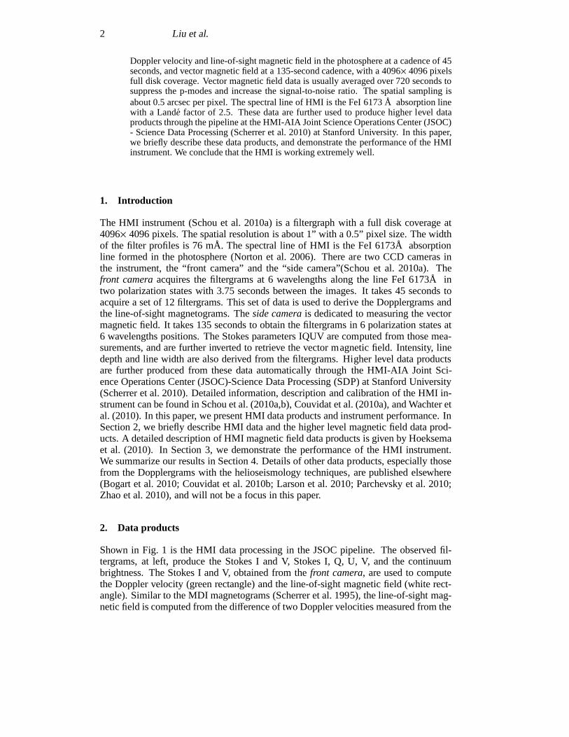
Shown in Fig. 1 is the HMI data processing in the JSOC pipeline. The observed fil-tergrams, at left, produce the Stokes I and V, Stokes I, Q, U, V, and the continuumbrightness. The Stokes I and V, obtained from thefront camera, are used to computethe Doppler velocity (green rectangle) and the line-of-sight magnetic field (white rect-angle). Similar to the MDI magnetograms (Scherrer et al. 1995), the line-of-sight mag-netic field is computed from the difference of two Doppler velocities measured from the

A First Look At Magnetic Field Data Products From HMI/SDO 3

Figure 1. The diagram of the HMI data processing in the JSOC pipeline. TheStokes parameters I and V, and Stokes parameters I, Q, U, V, are directly derivedfrom the observed filtergrams. The continuum brightness is calculated from the fil-tergrams. The Dopplergrams and the line-of-sight magnetograms are computed fromthe Stokes I and V, and the full disk vector magnetic field is derived from the StokesI, Q, U, V. These data are further processed to produce the high level data products,which are listed in the right column.

left and right circular polarizations. As an input, the Doppler velocity further produceshigher level data products that are listed in the orange and purple rectangles in the rightcolumn (rows 1-7). These data products are normally used forthe research purposes ofhelioseismology. The line-of-sight magnetograms are mapped on various coordinatessystems for further uses that are described later in Section2.1. The Stokes I, Q, U, Vfrom theside camera(pink rectangle in the second column) are derived from the fil-tergrams at a cadence of 135 seconds, or from the filtergrams averaged over a certaintime interval (currently a 720-second average) to suppressthe p-modes and increase thesignal-to-noise ratio. This average needs extra filtergrams before and after the expectedtemporal window because the filtergrams need to be interpolated onto a regular andfiner grid before averaging. For the 720-second average, thetemporal window used isactually 1215 seconds. The weights for the extra data are different from the rest of thedata. These Stokes parameters are inverted to obtain the vector magnetic field. Thevector magnetic field data further produce higher level dataproducts that are listed inthe pink rectangles in the right column (rows 9-11), which are described in Section 2.2.Usually the Doppler velocity and line-of-sight magnetic field are also computed fromthe averaged Stokes I and V using the same algorithm as that for the front cameradata.The continuum brightness (“brightness images”) in the yellow rectangle at the bottomis a derived product computed from the filtergrams, since true continuum is not sampledin the standard filtergram sets from either camera.

4 Liu et al.

Figure 2. The data processing map for the line-of-sight magnetic field data prod-ucts. The white and green rectangles represent the temporary and archived dataproducts, respectively. The pink rectangles with black shadow denote the names ofthe JSOC modules that produce the products. The parenthetical abbreviations hererefer to the institutions developing the codes. The diagramat the left shows thedefinitive data products; at the right are the near-real-time (NRT) data products (orthe quick-look data products).

Figure 3. Same as Fig. 2, but for the vector magnetic field dataproducts.

There are two categories for the HMI data, the near-real-time (NRT) data (quick-look data) and the definitive data. The NRT data are usually available within minutesafter the data are acquired. The main purposes of the NRT dataare monitoring the


Figure 4. The active regions are automatically identified inthe JSOC.Left:A line-of-sight magnetogram taken on March 29, 2010. The active region, AR11057, wasidentified, and bounded by a rectangle.Right: The vector magnetic field of thisactive region derived by VFISV. From top to bottom are inclination, azimuth, andstrength of the vector magnetic field. The 180o degree ambiguity of the azimuth issolved. The scale of x- and y-axis is 0.5” per pixel.

instrument and providing information for space weather forecast. Most NRT data aretemporary and will be removed later. The definitive data willbe archived. They consistof three different types of data products: the standard, the on-demand, and the on-request. The standard data products are completed on regular cadence about one dayafter the data are acquired; the on-demand data products arecompleted for a smallfraction of data when interesting things such as flares happen or whenever requested bya user; the on-request data products will be generated as resources allow, and completedwhen the system resources allow. In the following sections,we describe the line-of-sight magnetic field data products (Section 2.1), the vectormagnetic field data products(Section 2.2), and show examples of the data products (Section 2.3).

Figure 5. Left: The vector magnetic field of AR11057 deprojected to the helio-graphic coordinates with the Mercator projection method. The image is the verticalmagnetic field, and the arrow represents the horizontal field. Only the field withthe vertical component greater than 100 G is plotted here.Right: The non-linearforce-free field modeling of the active region AR11060 at 02:00 UT of April 8, 2010computed from the HMI vector magnetic field data. The algorithm used here was de-veloped by Wheatland et al. (2000); Wiegelmann (2004); Wiegelmann et al. (2006).The vector field data was pre-processed, as proposed by Wiegelmann et al. (2006).

6 Liu et al.

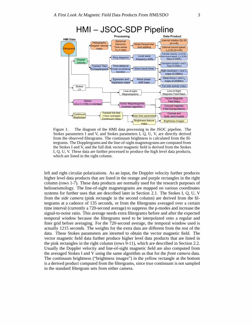
Figure 6. First test run result of the DAVE4VM (Schuck 2008) module on an HMIvector field data series.Left: One of the input vector magnetic field data of the activeregion AR11084 on July 1, 2010. The background image is the vertical componentof magnetic field with negative field in black and positive field in white. The bluearrows denote the horizontal field.Right: The derived horizontal flow velocity inorange arrows. The background image is again the vertical magnetic field.

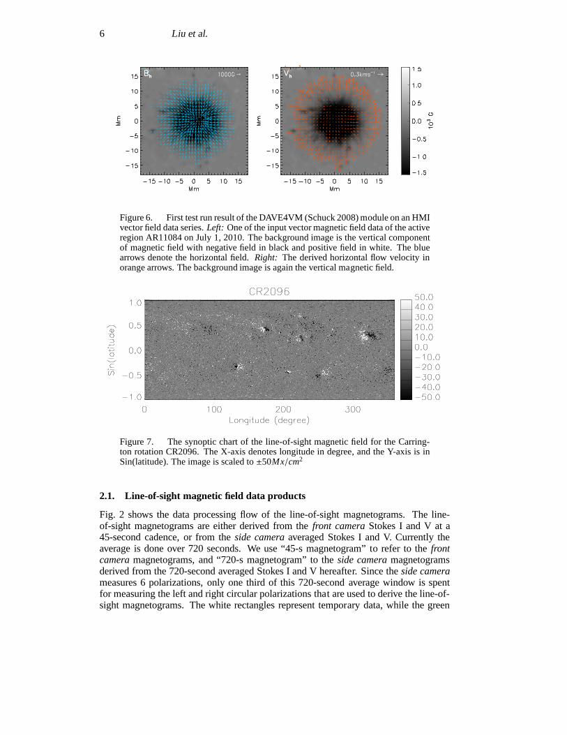
Figure 7. The synoptic chart of the line-of-sight magnetic field for the Carring-ton rotation CR2096. The X-axis denotes longitude in degree, and the Y-axis is inSin(latitude). The image is scaled to±50Mx/cm2

2.1. Line-of-sight magnetic field data products

Fig. 2 shows the data processing flow of the line-of-sight magnetograms. The line-of-sight magnetograms are either derived from thefront cameraStokes I and V at a45-second cadence, or from theside cameraaveraged Stokes I and V. Currently theaverage is done over 720 seconds. We use “45-s magnetogram” to refer to thefrontcameramagnetograms, and “720-s magnetogram” to theside cameramagnetogramsderived from the 720-second averaged Stokes I and V hereafter. Since theside camerameasures 6 polarizations, only one third of this 720-secondaverage window is spentfor measuring the left and right circular polarizations that are used to derive the line-of-sight magnetograms. The white rectangles represent temporary data, while the green


rectangles represent archived data that include the standard, the on-demand and theon-request data products. The pink rectangles with black shadow denote the pipelinemodules that produce the products. The parenthetical abbreviations here refer to theinstitutions developing the codes. On the left are the definitive line-of-sight field dataproducts, and on the right are the NRT data products. The definitive data productsinclude various synoptic maps and magnetogram movies. Alsoincluded are the coro-nal and heliospheric structures modeled by a Potential Field Source Surface (PFSS)model (Schatten et al. 1969; Altschuler & Newkirk 1969; Hoeksema et al. 1982), ora 3D MHD simulation (Hayashi 2005). Solar wind speed and the polarity of the in-terplanetary magnetic field computed from synoptic maps using the empirical Wang-Sheeley-Arge (WSA) model (Wang & Sheeley 1990; Arge & Pizzo 2000), surface flowinferred from time-series magnetograms using the algorithm FLCT (Fisher & Welsch2008), and patches of the active regions identified and bounded by a feature recogni-tion model (Turmon et al. 2002), are also given here. The NRT data products includesynoptic maps and magnetogram movies. More NRT data products, such as corona andheliosphere modeling and solar wind speed, may also be produced.

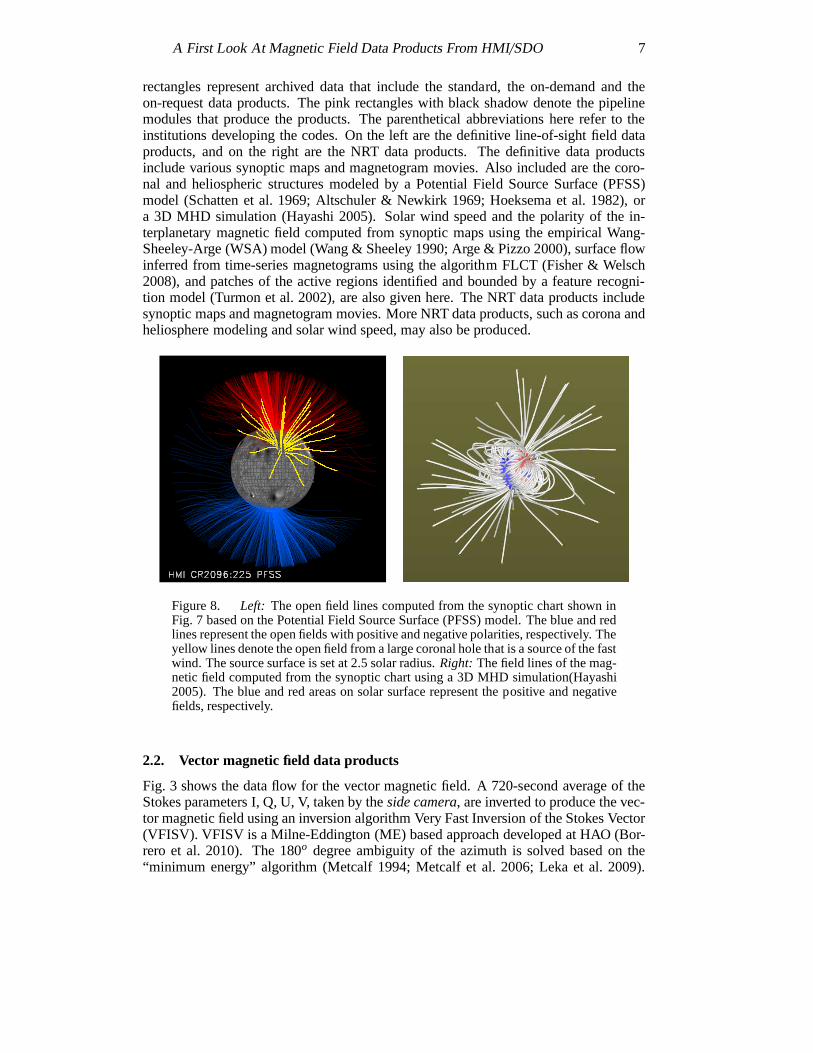
Figure 8. Left: The open field lines computed from the synoptic chart shown inFig. 7 based on the Potential Field Source Surface (PFSS) model. The blue and redlines represent the open fields with positive and negative polarities, respectively. Theyellow lines denote the open field from a large coronal hole that is a source of the fastwind. The source surface is set at 2.5 solar radius.Right: The field lines of the mag-netic field computed from the synoptic chart using a 3D MHD simulation(Hayashi2005). The blue and red areas on solar surface represent the positive and negativefields, respectively.

2.2. Vector magnetic field data products

Fig. 3 shows the data flow for the vector magnetic field. A 720-second average of theStokes parameters I, Q, U, V, taken by theside camera, are inverted to produce the vec-tor magnetic field using an inversion algorithm Very Fast Inversion of the Stokes Vector(VFISV). VFISV is a Milne-Eddington (ME) based approach developed at HAO (Bor-rero et al. 2010). The 180o degree ambiguity of the azimuth is solved based on the“minimum energy” algorithm (Metcalf 1994; Metcalf et al. 2006; Leka et al. 2009).

8 Liu et al.

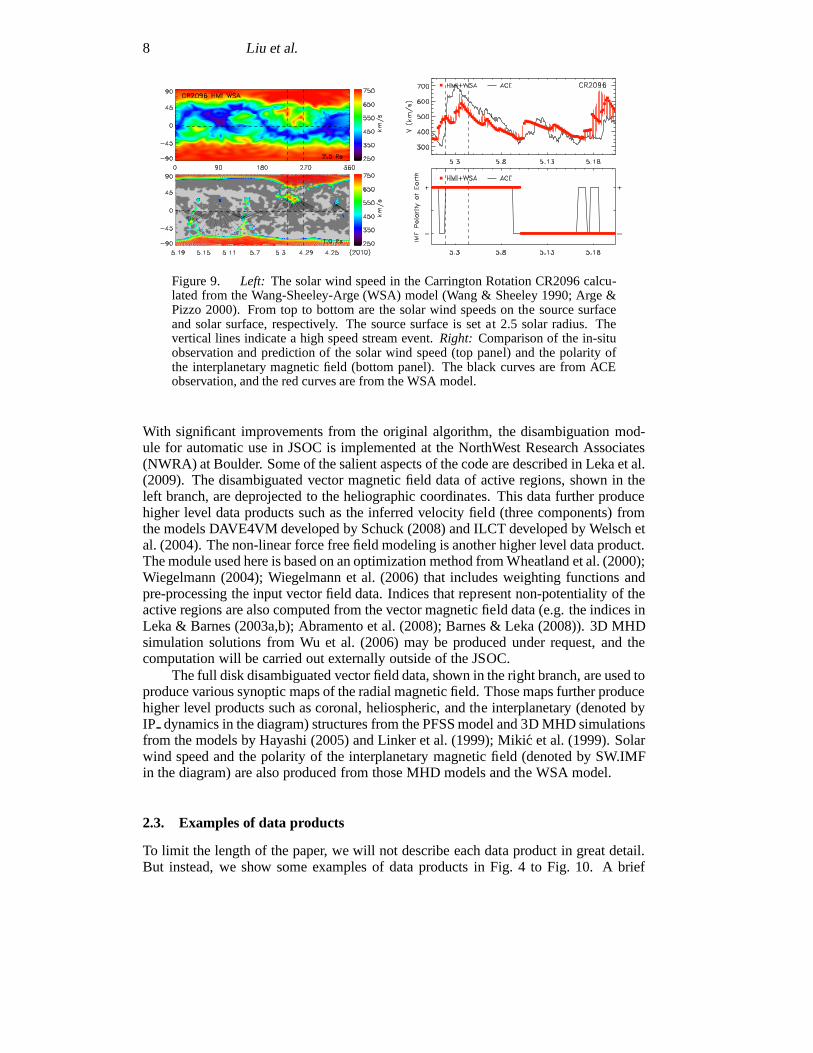
Figure 9. Left: The solar wind speed in the Carrington Rotation CR2096 calcu-lated from the Wang-Sheeley-Arge (WSA) model (Wang & Sheeley 1990; Arge &Pizzo 2000). From top to bottom are the solar wind speeds on the source surfaceand solar surface, respectively. The source surface is set at 2.5 solar radius. Thevertical lines indicate a high speed stream event.Right: Comparison of the in-situobservation and prediction of the solar wind speed (top panel) and the polarity ofthe interplanetary magnetic field (bottom panel). The blackcurves are from ACEobservation, and the red curves are from the WSA model.

With significant improvements from the original algorithm,the disambiguation mod-ule for automatic use in JSOC is implemented at the NorthWestResearch Associates(NWRA) at Boulder. Some of the salient aspects of the code aredescribed in Leka et al.(2009). The disambiguated vector magnetic field data of active regions, shown in theleft branch, are deprojected to the heliographic coordinates. This data further producehigher level data products such as the inferred velocity field (three components) fromthe models DAVE4VM developed by Schuck (2008) and ILCT developed by Welsch etal. (2004). The non-linear force free field modeling is another higher level data product.The module used here is based on an optimization method from Wheatland et al. (2000);Wiegelmann (2004); Wiegelmann et al. (2006) that includes weighting functions andpre-processing the input vector field data. Indices that represent non-potentiality of theactive regions are also computed from the vector magnetic field data (e.g. the indices inLeka & Barnes (2003a,b); Abramento et al. (2008); Barnes & Leka (2008)). 3D MHDsimulation solutions from Wu et al. (2006) may be produced under request, and thecomputation will be carried out externally outside of the JSOC.

The full disk disambiguated vector field data, shown in the right branch, are used toproduce various synoptic maps of the radial magnetic field. Those maps further producehigher level products such as coronal, heliospheric, and the interplanetary (denoted byIP dynamics in the diagram) structures from the PFSS model and 3D MHD simulationsfrom the models by Hayashi (2005) and Linker et al. (1999); Mikic et al. (1999). Solarwind speed and the polarity of the interplanetary magnetic field (denoted by SW.IMFin the diagram) are also produced from those MHD models and the WSA model.

2.3. Examples of data products

To limit the length of the paper, we will not describe each data product in great detail.But instead, we show some examples of data products in Fig. 4 to Fig. 10. A brief


description for each is given in the figure caption. A detailed description of the magneticfield data production can be found in the paper of Hoeksema et al. (2010).

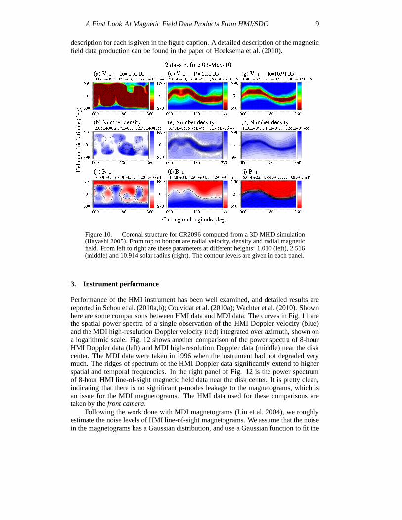
Figure 10. Coronal structure for CR2096 computed from a 3D MHD simulation(Hayashi 2005). From top to bottom are radial velocity, density and radial magneticfield. From left to right are these parameters at different heights: 1.010 (left), 2.516(middle) and 10.914 solar radius (right). The contour levels are given in each panel.

3. Instrument performance

Performance of the HMI instrument has been well examined, and detailed results arereported in Schou et al. (2010a,b); Couvidat et al. (2010a);Wachter et al. (2010). Shownhere are some comparisons between HMI data and MDI data. The curves in Fig. 11 arethe spatial power spectra of a single observation of the HMI Doppler velocity (blue)and the MDI high-resolution Doppler velocity (red) integrated over azimuth, shown ona logarithmic scale. Fig. 12 shows another comparison of thepower spectra of 8-hourHMI Doppler data (left) and MDI high-resolution Doppler data (middle) near the diskcenter. The MDI data were taken in 1996 when the instrument had not degraded verymuch. The ridges of spectrum of the HMI Doppler data significantly extend to higherspatial and temporal frequencies. In the right panel of Fig.12 is the power spectrumof 8-hour HMI line-of-sight magnetic field data near the diskcenter. It is pretty clean,indicating that there is no significant p-modes leakage to the magnetograms, which isan issue for the MDI magnetograms. The HMI data used for thesecomparisons aretaken by thefront camera.

Following the work done with MDI magnetograms (Liu et al. 2004), we roughlyestimate the noise levels of HMI line-of-sight magnetograms. We assume that the noisein the magnetograms has a Gaussian distribution, and use a Gaussian function to fit the

10 Liu et al.

0 1000 2000 3000 4000 5000 600010

2

103

104

105

106

107

108

degree l

pow

er

hmi Dopplermdi hi−res Doppler

Figure 11. Spatial power spectra of snapshots near disk center of the HMI Dopplerdata and MDI high-resolution Doppler data integrated over azimuth, shown on alogarithmic scale.

distribution of the low-field pixels of the magnetograms. The stars in Fig. 13 are thedistributions of the on-disk pixels of a 45-s magnetogram from thefront camera(left)and a 720-s magnetogram (right) from theside cameraversus magnetic field. Only thepixels with a value within -200 to 200 Mx/cm2 are selected. The number of the pixelsis normalized. The solid lines are the Gaussian functions that fit the distributions. Thenoise for the 45-s magnetogram, taken to be the sigma of the best-fit Gaussian, is 10.2Mx/cm2, and 6.3 Mx/cm2 for the 720-s magnetogram. As a comparison, by using thesame method, the noise for the MDI 1-minute magnetograms is 16.1 Mx/cm2, and 9.7Mx/cm2 for the 5-minute magnetograms(Liu et al. 2004).

HMI and MDI magnetograms have been further compared pixel bypixel. Thescatter plot in the left panel of Fig. 14 shows a comparison between HMI 45-s magne-tograms and 720-s magnetograms. The alignment is done basedon the location of thesolar disk center in the magnetograms. A 0.1 degree offset of the position angle in the45-s magnetograms is corrected. This comparison includes 14 pairs of 45-s and 720-smagnetograms. Each pair of magnetograms was taken at the same time. The solid linein the plot is a linear fit to the data. The slope is 0.98, and thezero point offset is sig-nificantly small, only 0.013. On the right is a comparison between MDI and HMI 45-smagnetograms. The comparison was done with 24 pairs of magnetograms. Each pair ofmagnetograms was taken at the same time. The HMI magnetograms were degraded tothe MDI resolution by convolving a 2D Gaussian function. Thewidth of the Gaussian


a)

degree l

ν m

Hz

0 3000 60000

2

4

6

8

10

log

pow

er

3

4

5

6

7

8

9 b)

degree l

ν m

Hz

0 3000 60000

1

2

3

4

5

6

7

8

log

pow

er

3

4

5

6

7

8

9

c)

degree l

ν m

Hz

0 3000 60000

2

4

6

8

10

log

pow

er

1

1.5

2

2.5

3

3.5

4

4.5

5

5.5

6

Figure 12. The spectrum of 8-hour HMI Dopplergrams near the disk center (left),compared with the spectrum of 8-hour MDI high resolution Dopplergrams near thedisk center (middle) taken in 1996. The ridges of HMI Dopplerspectrum extendsinto higher temporal and spatial frequencies. In the right panel is the spectrum of8-hour HMI line-of-sight magnetic field data near the solar disk center. It is prettyclean, indicating no significant leakage of the p-modes to the magnetograms.

is the ratio of the MDI and HMI pixel sizes. A -0.22 degree offset of the position anglein the MDI magnetograms is corrected. The offset of the position angle in the HMI 45-smagnetograms is corrected, too. The slope of a linear fit to the data, shown in the solidblack line in the plot, is 1.2, implying that the line of sightpixel-averaged magneticsignal inferred from MDI data is greater than that derived from the HMI front cameradata by a factor of 1.2. There is also an outstanding zero point offset between them. Acomparison of 24 pairs of MDI magnetograms and HMI 720-s magnetograms (beingnot shown here) gives a slope of 1.2, too. A boxcar average wasalso tested to degradeHMI’s spatial resolution. The result is very similar.

The quality of data towards the solar disk limb is also examined. Fig. 15 showsan area of the Sun from 60 degree north to the north pole from a MDI 1-minute mag-netogram (left), a HMI 45-s magnetogram (middle), and a HMI 720-s magnetogram(right). Many small-scale magnetic elements that are not visible in the MDI magne-togram are clearly seen in the HMI magnetograms.

A time series profile of the mean solar magnetic field is shown in Fig. 16. Themean field from WSO is measured with integrated sunlight in a mode of measuring theSun-as-a-star. The WSO mean field plotted here is multipliedby a factor of 1.8 for thesaturation correction (Svalgaard et al. 1978). The “mean field” from the MDI and HMI,on the other hand, is derived from the full disk line-of-sight magnetograms by simply

12 Liu et al.

Figure 13. Estimate of the noise level for the line-of-sightmagnetograms. Herewe assume that the noise has a Gaussian distribution, and usea Gaussian functionto fit the distribution of the low-field pixels of the magnetograms. Left: The starsare the distribution of the pixels selected from a 45-s magnetogram over the Sun’sdisk, and the solid line is a Gaussian function that fits the distribution. The numberof pixels is normalized. The sigma of the Gaussian (width) is10.2 Mx/cm2, and theshift of the Gaussian peak is 0.06 Mx/cm2. Right: Same as that in the left panel, butfor a 720-s magnetogram. The sigma is 6.3 Mx/cm2 and the shift of the Gaussianpeak is 0.08 Mx/cm2.

Figure 14. Comparison of the line-of-sight magnetograms taken by the two cam-eras of HMI (left) and by the HMIfront cameraand MDI (right). Left: Scatter plotof 14 pairs of 45-s and 720-s magnetograms taken in June-August 2010. Each pairof magnetograms was taken at the same time. The solid line is alinear fit to the data.Right: Scatter plot of 24 pairs of HMI 45-s and MDI magnetograms taken in June-August 2010. Each pair was taken at the same time. The HMI magnetograms aredegraded to the MDI spatial resolution by convoling a 2D Gaussian function. Thesolid line is a linear fit to the data.


Figure 15. Solar north pole observed by MDI and HMI on September 11, 2010.From left to right are MDI magnetogram, HMI 45-s magnetogram, and HMI 720-smagnetogram. The region is from 60 degree north to the north pole. The images areall scaled to±50Mx/cm2

Figure 16. The mean solar magnetic field from 2010 May 1 to June12. The“mean field” from HMI and MDI is derived by summing the line-of-sight magneticfield over the solar disk. The black crosses and the green diamonds are the “meanfield” computed from the HMI 45-s and 720-s magnetograms. Theblue stars arecalculated from the MDI magnetograms. The red dots are the mean field measuredat WSO, multiplied by a factor of 1.8.

summing up the magnetic field over the solar disk. It differs from the real mean fieldbecause it doesn’t take into account the solar intensity. Itis seen that they match wellin general, but the mean field from MDI data shows a slight shift to the negative field,implying that there might be a systematic offset of the zero point of magnetic field in theMDI magnetograms in that time interval though the offset of each MDI magnetogramhas been corrected (Liu et al. 2004). Further investigationis needed.

As a demonstration of evolution of active regions, we show inFig. 17 the snap-shots of the line-of-sight magnetic field of two emerging active regions, AR11069 andAR11072. An outstanding difference between these two regions is the complexity of themagnetic field structure: there are multiple positive and negative field patches emergingin AR11069, while only two patches with opposite polaritiesin AR11072. The solaractivities are also different: AR11069 produced 7 C-class and 1 M-class flares during

14 Liu et al.

Figure 17. Snapshots of the line-of-sight magnetic field of the active regionAR11069 for a 48-hour interval during the rapidly growing phase (top panels), andthe AR11072 for a 100-hour interval during the growing phase(bottom panels). Thefield of view of each image is 150”×120”. The images are all scaled to±250Mx/cm2

There are multiple emerging flux patches in AR11069, which are marked by N1-3and S1-3, while only two patches with opposite polarities emerged in AR11072.

Figure 18. The time profiles of the pseudo-fluxes for the emerging active regionAR11069 from 2010 May 3 to May 8. The unsigned pseudo-flux (thick black curve),positive pseudo-flux (thin black curve), and negative pseudo-flux (red curve) aremeasured from the 45-s magnetograms. The blue curve shows the 5-minute aver-aged GOES X-ray flux. This plot shows that the active region produced its firstC-class flare after 20 hours of the initial emerging, and tookanother 14 hours beforeproducing three more C-class (or above) flares. After this activity, the emergenceapparently stopped, and 36 hours later another C-class flarewas produced.

its disk passage, while AR11072 did not produce any C-class or above flares (fromhttp://www.swpc.noaa.gov/). To show their emerging in more detail, we plot a timeseries of a “pseudo-flux” of AR11069 (Fig. 18) and AR11072 (Fig. 19). The “pseudo-flux”, computed from the line-of-sight magnetograms by assuming the field is purelyradial, is defined to be

∑i Bi

los×Si/cos(µi ), whereBilos is the line-of-sight field at pixel

i, Si is the area this pixel covers, andµi is the center-to-limb angle. The real magnetic


Figure 19. Same as Fig. 18 but for the active region AR11072 from 2010 May20 to 25. Again, it is an emerging active region. But it did notproduce any C-classor above flares during its disk passage.

flux could be computed from the vector magnetic field data thatwill be available soon.It shows that both underwent a quick emerging phase, and their sizes are very similar.Continuing analysis with HMI vector magnetic field data could bring new insight tohelp understand why their activities are so different.

4. Conclusions

In this paper, we briefly describe the HMI magnetic field data products, and presentanalyses to demonstrate the performance of the HMI instrument. We conclude that theHMI is working extremely well.

Acknowledgments. We wish to thank many many others who have been mak-ing great contributions to this mission! This work was supported by NASA ContractNAS5-02139 (HMI) to Stanford University. The disambiguation module (NWRA) wasimproved through additional support by NASA GI contract NNH09CF22C. The re-search of the feature recognition described in this paper was carried out in part by theJet Propulsion Laboratory, California Institute of Technology, under a contract withNASA.

References

Abramenko, V. Yurchyshyn, V., Wang, H., 2008, ApJ, 681, 1669.Altschuler, M. D., Newkirk, G., Jr. 1969, Solar Phys., 9, 131.Arge, C. N., Pizzo, V. J.,JGR, 2000, 105, 10465.Barnes, G., Leka, K. D., ApJ, 2008, 688, 107.Bogart, R., et al., Solar Phys., 2010, in preparation.Borrero, J. M., Tomczyk, S., Kubo, M., Socas-Navarro, H., Schou, J., Couvidat, S., Bogart, R.,

Solar Phys., 2010, in press.Couvidat, S., et al., Solar Phys., 2010a, in preparation.Couvidat, S., Zhao, J., Birch, A. C., Kosovichev, A. G., Duvall, T. L., Parchevsky, K., Scherrer,

P. H., Solar Phys., 2010b, in press.

16 Liu et al.

Fisher, G. H., Welsch, B. T.: 2008, In: Howe, R., Komm, R.W., Balasubramaniam, K.S., Petrie,G.J.D. (eds.),Subsurface and Atmospheric Influences on Solar Activity, ASP Conf. Ser.383, 373.

Hayashi, K., ApJS, 2005, 161, 480.Hoeksema, J. T., Wilcox, J. M., Scherrer, P. H. 1982,JGR, 87, 10331.Hoeksema, J. T., et al. Solar Phys., 2010, in preparation.Larson, T., et al. Solar Phys., 2010, in preparation.Leka, K. D., Barnes, G., ApJ, 2003a, 595, 1277.Leka, K. D., Barnes, G., ApJ, 2003b, 595, 1296.Leka, K. D., Barnes, G., Crouch, A. D., Metcalf, T. R., Gary, G. A., Jing, J., Liu, Y., Solar Phys.,

2009, 260, 83.Linker, J. A., Mikic, Z., Biesecker, D. A., Forsyth, R. J., Gibson, S. E., Lazarus, A. J., Lecinski,

A., Riley, P., Szabo, A., Thompson, B. J.,JGR, 1999, 104, 984.Liu, Y., Zhao, X-P, Hoeksema, J. T., Solar Phys., 2004, 219, 39.Metcalf, T. R., Solar Phys., 1994, 155, 235.Metcalf, T. R., Leka, K. D., Barnes, G. Lites, B. W., Georgoulis, M. K., Pevtsov, A. A., Bala-

subramaniam, K. S., Gary, G. A., Jing, J., Li, J., Liu, Y., Wang, H. N., Abramenko, V.,Yurchyshyn, V., Moon, Y.-J., Solar Phys., 2006, 237, 267.

Mikic, Z., Linker, J. A., Schnack, D. D., Lionello, R., Tarditi, A., Physics of Plasma, 1999, 6,2217.

Norton, A. A., Graham, J. Pietarila, Ulrich, R. K., Schou, J., Tomczyk, S., Liu, Y., Lites, B.W., Lopez Ariste, A., Bush, R. I., Socas-Navarro, H., Scherrer, P. H., Solar Phys., 2006,239, 69.

Parchevsky, K., et al. Solar Phys., 2010, in preparation.Schatten, K. H., Wilcox, J. M., Ness, N. F. 1969, Solar Phys.,6, 442.Scherrer, P. H., Bogart, R. S., Bush, R. I., Hoeksema, J. T., Kosovichev, A. G., Schou, J.,

Rosenberg, W., Springer, L., Tarbell, T. D., Title, A., Wolfson, C. J., Zayer, I., and MDIEngineering Team, 1995, Solar Phys., 162, 129.

Scherrer, P. H., Schou, J., Solar Phys., 2010, in preparation.Scherrer, P. H., et al., Solar Phys., 2010, in preparation.Schou, J., et al., Solar Phys., 2010a, in preparation.Schou, J., Borrero, J. M., Norton, A. A., Tomczyk, S., Elmore, D., Card, G. L., Solar Phys.,

2010b, in press.Schuck, P. W., ApJ, 2008, 683, 1134.Svalgaard, L., Duvall, T. L., Jr., Scherrer, P. H., Solar Phys., 1978, 58, 225.Turmon, M., Pap, J. M., Mukhtar, S., ApJ, 2002, 568, 396.Welsch, B. T., Fisher, G. H., Abbett, W. P., Regnier, S., ApJ,2004, 610, 1148.Wheatland, M. S., Sturrock, P. A., Roumeliotis, G., ApJ, 2000, 540, 1150.Wiegelmann, T., Solar Phys., 2004, 219, 87.Wiegelmann, T., Inhester, B., Sakurai, T., Solar Phys., 2006, 233, 215.Wachter, R. et al., Solar Phys., 2010, in preparation.Wang, Y.-M.; Sheeley, N. R., Jr., ApJ, 1990, 355, 726.Wu, S. T., Wang, A. H., Liu, Y., Hoeksema, J. T., ApJ, 2006, 652, 800.Zhao, J., et al., Solar Phys., 2010, submitted.

a first look at magnetic field data products from hmi...

Documents