A First Look at Class Incremental Learning inDeep Learning Mobile Traffic Classification

Giampaolo Bovenzi†, Lixuan Yang, Alessandro Finamore,Giuseppe Aceto†, Domenico Ciuonzo†, Antonio Pescape†, Dario Rossi

Huawei Technology France, † University of Napoli Federico II

Abstract—The recent popularity growth of Deep Learning (DL)re-ignited the interest towards traffic classification, with severalstudies demonstrating the accuracy of DL-based classifiers toidentify Internet applications’ traffic. Even with the aid ofhardware accelerators (GPUs, TPUs), DL model training remainsexpensive, and limits the ability to operate frequent modelupdates necessary to fit to the ever evolving nature of Internettraffic, and mobile traffic in particular. To address this pain point,in this work we explore Incremental Learning (IL) techniquesto add new classes to models without a full retraining, hencespeeding up model’s updates cycle. We consider iCarl, a state ofthe art IL method, and MIRAGE-2019, a public dataset with trafficfrom 40 Android apps, aiming to understand if there is a case forincremental learning in traffic classification. By dissecting iCarlinternals, we discuss ways to improve its design, contributinga revised version, namely iCarl+. Despite our analysis revealstheir infancy, IL techniques are a promising research area on theroadmap towards automated DL-based traffic analysis systems.

I. INTRODUCTION

Traffic classification (TC) is at the core of any networktraffic monitoring system, and a pillar for traffic management,cyber security, quality-of-experience monitoring, and otherstrategic activities for network operators. It is also a verymature research topic with many surveys on the subject [1–3].

From a chronological standpoint, we can categorize TCliterature into two “waves”. The first wave ignited in the early2000’s, and centered around the use of Machine Learning(ML) methods using per-packet (e.g., packet size, packetsinter-arrival time) or per-flow (e.g., total bytes, packets, ports)features as input targeting the classification of a handful ofapplications. Several works demonstrated that even when justa few packets of a flow were observed, the classification wasaccurate [4, 5], and could be sustained at line-rate speed [6]—“early” TC was born.

Inspired by the success of image processing in computervision, in the last years Deep Learning (DL) techniquesre-ignited the interest towards TC, with several DL-basedclassifiers being proposed using as input either raw payloadbytes or the same traffic features discovered during the firstwave [7–12]. This renewed interest stems also from the growthin adoption of traffic encryption, the extreme dynamicity ofInternet traffic, and the heterogeneity of devices connecting tothe Internet, especially when considering mobile ones (havingan ecosystems of tools that eases the installation of new appsand their updates) [11].

Accordingly, to closely track the network traffic landscape,an effective TC system should support continuous model

ML / DLNetwork

Monitoringtrain

label

sample

test

deplo

y monitor

log

alert

Fig. 1: Models development infinite loop.

updates, as sketched in Fig. 1. Incremental Learning (IL), alsoknown as continuous or online learning [13], is a disciplinestudying how to update models to accommodate the newknowledge required to perform well the target task (e.g., anew class needs to be added to a classifier). This fits wellTC needs, and a few works indeed consider incremental TC.However, those works resort to datasets with only a few classes(typically less than 10), they use per-flow features (which onlyenable post-mortem classification [14, 15]), and they do notconsider scenarios where new applications are progressivelyadded to models (needed to perform network management onnew services or apps). In other words, TC literature focusesonly on the problem of creating the most accurate classifiergiven a dataset where both (a) the number of classes and (b)the data for each class are immutable. In turn, TC systemsbased on literature approaches use amend and retrain policies:to add new applications or new traffic behavior to a model oneneeds to (i) create a new training set (or expand the existingone), and (ii) train a new model from scratch—model updatesare not incremental.

Differently, in this paper we investigate the use of IL tech-niques [13] to expand the knowledge of an existing DL-basedtraffic classifier without requiring a full retraining, namelyClass Incremental Learning (CIL), which we explore to sup-port real-world operations by reducing the requirement of fullmodels retraining. We apply iCarl [16], a CIL state-of-the-art approach, to a standard 1-dimensional convolutional neuralnetwork TC model, using the publicly available MIRAGE-2019dataset comprising traffic of 40 popular Android applications.Our contributions are two-fold: (i) we dissect iCarl’s designand propose alternative options, including a revised version ofthe original method we named iCarl+, and (ii) a thoroughevaluation highlighting relevant trends, pitfalls, and further

arX

iv:2

107.

0446

4v1

[cs

.NI]

9 J

ul 2

021

time

tn tn+1

modelweight

time

tn+1

wa wb wc wd

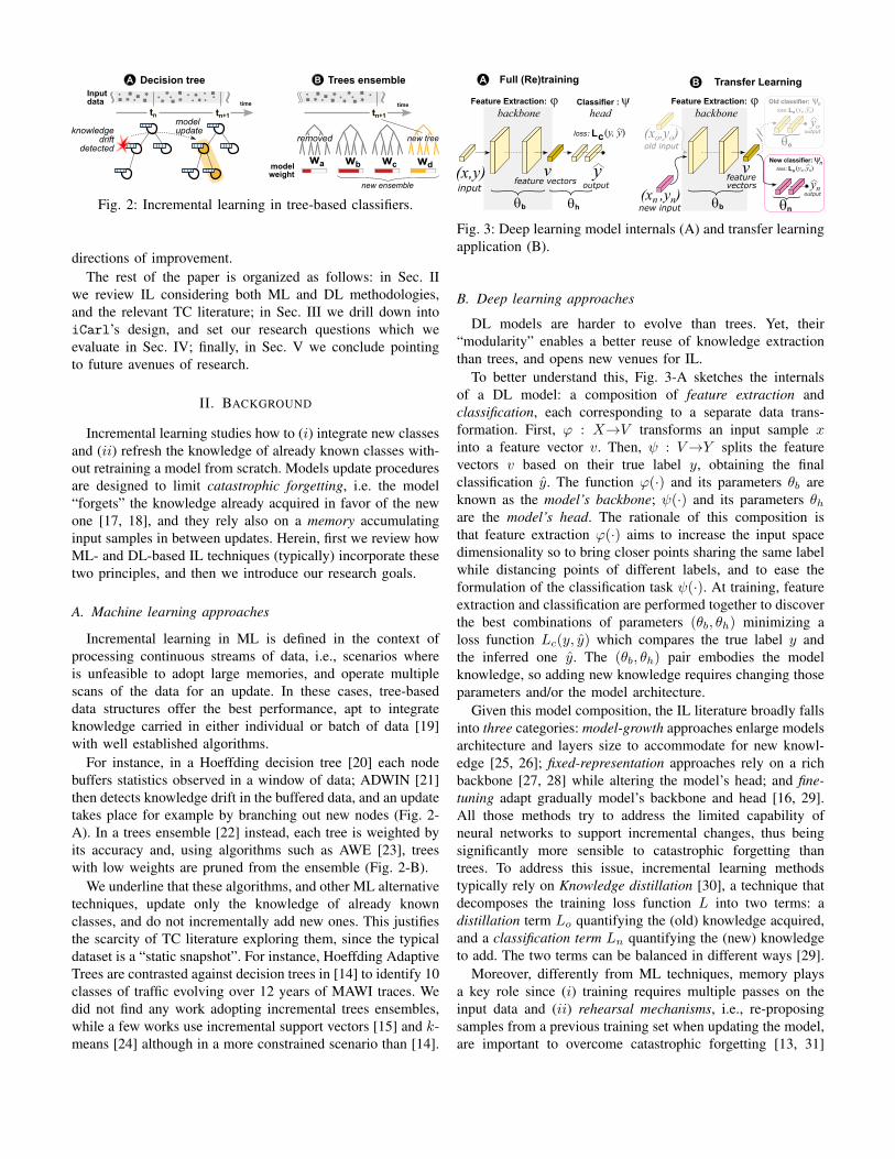
A Decision tree B Trees ensemble

knowledge drift

detected

Inputdata

modelupdate

new tree

new ensemble

removed

Fig. 2: Incremental learning in tree-based classifiers.

directions of improvement.The rest of the paper is organized as follows: in Sec. II

we review IL considering both ML and DL methodologies,and the relevant TC literature; in Sec. III we drill down intoiCarl’s design, and set our research questions which weevaluate in Sec. IV; finally, in Sec. V we conclude pointingto future avenues of research.

II. BACKGROUND

Incremental learning studies how to (i) integrate new classesand (ii) refresh the knowledge of already known classes with-out retraining a model from scratch. Models update proceduresare designed to limit catastrophic forgetting, i.e. the model“forgets” the knowledge already acquired in favor of the newone [17, 18], and they rely also on a memory accumulatinginput samples in between updates. Herein, first we review howML- and DL-based IL techniques (typically) incorporate thesetwo principles, and then we introduce our research goals.

A. Machine learning approaches

Incremental learning in ML is defined in the context ofprocessing continuous streams of data, i.e., scenarios whereis unfeasible to adopt large memories, and operate multiplescans of the data for an update. In these cases, tree-baseddata structures offer the best performance, apt to integrateknowledge carried in either individual or batch of data [19]with well established algorithms.

For instance, in a Hoeffding decision tree [20] each nodebuffers statistics observed in a window of data; ADWIN [21]then detects knowledge drift in the buffered data, and an updatetakes place for example by branching out new nodes (Fig. 2-A). In a trees ensemble [22] instead, each tree is weighted byits accuracy and, using algorithms such as AWE [23], treeswith low weights are pruned from the ensemble (Fig. 2-B).

We underline that these algorithms, and other ML alternativetechniques, update only the knowledge of already knownclasses, and do not incrementally add new ones. This justifiesthe scarcity of TC literature exploring them, since the typicaldataset is a “static snapshot”. For instance, Hoeffding AdaptiveTrees are contrasted against decision trees in [14] to identify 10classes of traffic evolving over 12 years of MAWI traces. Wedid not find any work adopting incremental trees ensembles,while a few works use incremental support vectors [15] and k-means [24] although in a more constrained scenario than [14].

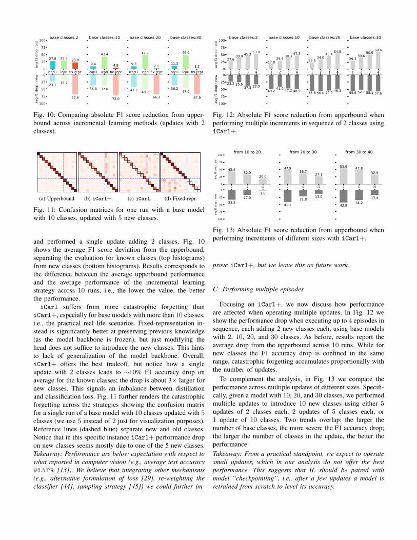
input outputfeature vectors

Full (Re)training

Classifier :

Lc

�b �h

A

(x,y) yv

Feature Extraction: � �backbone head

loss: (y, y)

Transfer LearningB

�New classifier:

o

�nnew input(xn ,yn)

old input(xo,yo)

Loloss: (yo ,yo)

outputyo

Lnloss: (yn ,yn)

Old classifier: �o

�n

outputyn

�b

featurevectors

v

Feature Extraction: �backbone

Fig. 3: Deep learning model internals (A) and transfer learningapplication (B).

B. Deep learning approaches

DL models are harder to evolve than trees. Yet, their“modularity” enables a better reuse of knowledge extractionthan trees, and opens new venues for IL.

To better understand this, Fig. 3-A sketches the internalsof a DL model: a composition of feature extraction andclassification, each corresponding to a separate data trans-formation. First, ϕ : X→V transforms an input sample xinto a feature vector v. Then, ψ : V→Y splits the featurevectors v based on their true label y, obtaining the finalclassification y. The function ϕ(·) and its parameters θb areknown as the model’s backbone; ψ(·) and its parameters θhare the model’s head. The rationale of this composition isthat feature extraction ϕ(·) aims to increase the input spacedimensionality so to bring closer points sharing the same labelwhile distancing points of different labels, and to ease theformulation of the classification task ψ(·). At training, featureextraction and classification are performed together to discoverthe best combinations of parameters (θb, θh) minimizing aloss function Lc(y, y) which compares the true label y andthe inferred one y. The (θb, θh) pair embodies the modelknowledge, so adding new knowledge requires changing thoseparameters and/or the model architecture.

Given this model composition, the IL literature broadly fallsinto three categories: model-growth approaches enlarge modelsarchitecture and layers size to accommodate for new knowl-edge [25, 26]; fixed-representation approaches rely on a richbackbone [27, 28] while altering the model’s head; and fine-tuning adapt gradually model’s backbone and head [16, 29].All those methods try to address the limited capability ofneural networks to support incremental changes, thus beingsignificantly more sensible to catastrophic forgetting thantrees. To address this issue, incremental learning methodstypically rely on Knowledge distillation [30], a technique thatdecomposes the training loss function L into two terms: adistillation term Lo quantifying the (old) knowledge acquired,and a classification term Ln quantifying the (new) knowledgeto add. The two terms can be balanced in different ways [29].

Moreover, differently from ML techniques, memory playsa key role since (i) training requires multiple passes on theinput data and (ii) rehearsal mechanisms, i.e., re-proposingsamples from a previous training set when updating the model,are important to overcome catastrophic forgetting [13, 31]

Feature Extractor :�backbone

�b

Nearest Mean Classifier (NMC)

�

�a �b

�(x)output

y

�h

featurevectors

v

new input(xn ,yn)

old input

(xo,yo)herdingselection

Ln+

: sigmoid activationg

enc(yn), gx( (

: (x ,y)Uunion

Lo gx , gx( (~loss:

pre-expanded output layer(units allocated but not used)

:

rehearsal

single layer

0 0 1

Fig. 4: Sketch of iCarl [16] internals.

and avoid the extra cost of data augmentation techniques likegenerative replay [32].Transfer learning.

A model’s backbone learns hidden patterns in the data,and the larger the training set (and the lower the layer inthe model’s architecture), the more the extracted knowledgeis expected to abstract from the specific classification taskat hand. This observation is key in transfer learning wherethe backbone of a model Ma is reused for a model Mb bydetaching Ma head θo and replacing it with a new one θntailored to the new classification task (Fig. 3-B). Then, Mb

is trained via fixed-representation or fine-tuning. ConsideringTC, the authors of [33] show that one can reuse the backboneof a model trained to predict flows duration and bandwidth,to train a classifier to distinguish 5 traffic classes.

In its basic formulation, transfer learning derives a newmodel from an existing one, hence does not perform anupdate. It is however also possible to incrementally add newtasks to an existing model [34]—this is known as multi-taskincremental learning. In this case, a new head is attached tothe backbone without pruning the existing ones. Consideringtraffic classification, in [35] authors study how to add a trafficclassifier task to a model trained to classify both flow durationand flow bandwidth.Class incremental learning (CIL).

If we do not stick to rigid taxonomy boundaries, transferlearning can also be used for CIL. To be more specific,a CIL state-of-the-art method is Incremental Classifier andRepresentation Learning (iCarl) [16]. iCarl is a fine-tuningtechnique using (i) known classes exemplars rehearsal, (ii)a pre-allocated output layer, (iii) knowledge distillation, and(iv) a Nearest Mean Classifier (NMC), as sketched in Fig. 4.

Let us consider a base model (θb, θh) trained on a (Xo, Yo)dataset and having C classes. At the input, iCarl selectsexemplars of known classes P⊆Xo which are rehearsed attraining. A herding mechanism [36] selects exemplars basedon their distance with respect to the class average centroid inthe latent space, and keeps them in a memory of fixed size.

At the output, the model’s head is a single layer (withneurons using the sigmoid activation function) of size K

with K�C—the head pre-allocates K-C units for futureclasses to be added. We denote with gx the response vec-tor associated to K sigmoids, whereas with g0x (resp. gfx)the subvector associated to the base C (resp. future K-C)classes. The classification is however operated computingdistance from classes’ average centroid µc in the latent spacey = argmini ‖ϕ(x)− µc‖—this is known as Nearest MeanClassifier (NMC). In computer vision, this simple mechanismhas been found superior to more typical parametric classi-fication (i.e., leveraging the model head) when performingincremental learning [37, 38].

When performing an update, iCarl first applies the currentmodel to both exemplars in memory and new classes data. Theobtained (C-dimensional) soft-output g0x is used for knowledgedistillation Lo(g

0x, g

0x). Additionally, some of the K-C extra

units pre-allocated in the model’s head (i.e. gfx), denoted withg1x, are “consumed” for the new classes. These units aretrained via the classification loss, whereas labels of new (resp.base) classes are one-hot (resp. zero-vector) encoded, namelyLn(enc(yn), g

1x).

C. Our research goal

We found scarce literature for IL applied to TC. Indeed,only [39] presents a closed-loop TC system, but authors (i)consider a small use-case with 10 classes, (ii) adopt simplefine-tuning to introduce new classes, and (iii) focus on a singlemodel update. Broadly speaking, the closely related literature,no matter the adopted methodology, share common limitations:old datasets ([15, 24] use data from 2005, whereas [14]use 2001-2014 data); very few (typically less than 10), andvery generic classes (HTTP, DNS, SSH, etc.); adopt per-flowfeatures, thus not performing early traffic classification. On theone hand, the validation of CIL techniques against outdateddatasets allow to grasp insights on models generalization andconjecture on their future longevity. On the other hand, somedatasets are 10+ years old, and offer just a handful of classes,which makes them unfit for our study. Indeed, the limitedavailability of public labeled datasets for TC is a well knownproblem, quite far from the abundance of datasets for computervision- and natural language processing-related tasks.

Methodology-wise, we aim to a fresh look at CIL fortraffic classification. We discard ML-based IL techniques sincethey can only expand knowledge of already known classes,and rely on handcrafted features. We also discard multi-tasktransfer learning techniques since they lead to multi headedmodels which complicate systems operation—given one inputsample, a multi headed model would return one label foreach head, raising the problem of how to reconcile multipleoutput labels into one. We focus instead on fine-tuning, andspecifically iCarl given its accuracy, limited complexity, andhigh scalability [16]. To the best of our knowledge, iCarlhas only been applied to image classification, hence we aimto understand if its qualities remain the same when used for(mobile) TC. To do so, we contribute an in-depth analysis ofiCarl internal design, challenging the original choices (e.g.,the adoption of NMC), and thoroughly evaluating alternative

choices using the publicly available MIRAGE-2019 which, tothe best of our knowledge, is the most recent dataset on mobiletraffic, and offer a large variety of classes (40 Android apps),thus fitting well the aim of our study.

III. METHODOLOGY

To better understand the design space, in this section westart reviewing iCarl internal components in more details,and set our research questions. We then introduce the dataset,and the DL-based model we use in our evaluation.

A. Dissecting iCarl designiCarl is a CIL state-of-the-art approach for image clas-

sification which trades off complexity and performance withrespect to alternative solutions like [40, 41], thus is the perfectcandidate technique for our initial exploration of CIL for TC.iCarl’s design centers around two components: a memory

at the input, and an NMC at the output (Fig. 4), both operatingon the feature vectors generated by a model’s backbone. Thememory is fixed in size, and contains a uniform amount ofexemplars for each class. It follows that, at each update,each known class drops the same amount of exemplars tomake room for the new classes exemplars. Such filtering iscontrolled by a herding mechanism, a procedure aiming toselect a subset of exemplars so that the class average centroidin the latent space created from the filtered exemplars isas close as possible to the one obtained without filtering—it selects a “herd” of points capturing “the body” of theclass (for more details, please refer to [16]). By design,an NMC tights to the same mechanics of centroids andpoint-to-centroid distances computation in the latent space.According to [16], these design choices aim to decouple thenon-linear feature extraction from the linear classifier: whilethe NMC approximates the class feature vectors mean, theherding selection process tries to keep this mean unchangedby carefully selecting exemplars—this is the representationlearning component in the iCarl acronym, which stresses theneed of a robust feature extraction.

At a closer look, we spot two other subtle aspects, at theborder between design choices and implementation details.First, iCarl adopts a sigmoid rather than a softmax activationfunction at the output. We find this peculiar, and while authorsbriefly state that both functions are equivalent, they do notevaluate the impact of softmax. Secondly, as introduced inSec. II-B, the output layer is pre-allocated, i.e., its size is largerthan the number of classes required, and the extra units areprogressively used when adding new classes. iCarl authorsdo not mention this in their paper, but it is evident inspectingiCarl source code.1 While at first sight this sounds like a“smart trick”, it can cause unexpected effects when intertwinedwith the use of sigmoid activations (see Sec. IV-A).

Considering the overall design choices, in this work wetarget the following questions:

• Is it better to use an NMC, or to classify via the outputlayer?

1https://github.com/srebuffi/iCaRL

1 6 11 16 21 26 31 36app rank

0

2000

4000

6000

8000

sam

ples

samples

0.0

0.2

0.4

0.6

0.8

1.0

CDF

cdf

Fig. 5: MIRAGE-2019 dataset composition.

• Is it better to adopt a sigmoid, or a softmax activationfunction at the output layer?

• Is it better to pre-allocate the output layer size, orprogressively expand it?

• How sensitive is the herding selection to memory size?Does a larger memory provide better performance?

These are all general questions of practical relevance, and tothe best of our knowledge they are not fully investigated in theliterature. Yet, it is beyond the scope of this work to providea final answer to them. Rather, we explore the questionsin the context of TC using only one dataset. In particular,differently from observed in [16], we find that (i) output layerclassification is superior to NMC, (ii) softmax is superior tosigmoid, (iii) pre-allocation of the output layer may have adetrimental effect, and (iv) memory has indeed an impact inbalancing catastrophic forgetting as reported in literature. Wecontribute our observations into a revised version of iCarl,namely iCarl+. As we shall see in Sec. IV-B, neither iCarlnor iCarl+ match the performance observed in computervision when tested on a TC dataset. Yet, iCarl+ significantlyreduces training time, another aspect not quantified in previousliterature (Sec. IV-E).

B. Dataset

In this work we use the MIRAGE-2019 [11] dataset. Itcontains traffic related to 40 Android apps belonging to16 different categories.2 MIRAGE-2019 was collected at theARCLAB laboratory of the University of Napoli “FedericoII” with multiple measurement campaigns running betweenMay 2017 and May 2019. In each experiment a volunteer(out of ≈300 students) was asked to use one of the 40 appswhile in background raw pcap files and strace log-fileswere collected on the phones. Then, pcap were converted intoJSON files where each record reports on the network activityof a different bidirectional flows (biflows) with aggregate levelmetrics (total bytes, packets, etc.), and per-packet level metrics(time series of packet size, direction, TCP flags, etc.). Thestrace logs instead exposed the socket-to-appID mappingas observed on the phone, so they were used as ground-truthto label the per-flow logs obtained from raw pcaps. For moredetails, please refer to [11].

The MIRAGE-2019 dataset contains ≈100k biflows dis-tributed across apps as shown in Fig. 5. Although the number

2http://traffic.comics.unina.it/mirage/app list.html

0 10 20 30 40 50 60 70 80 90packet index

0

10

20

30app

inde

x

500

1000

avg

pack

et si

ze

0 10 20 30 40 50 60 70 80 90packet index

0

10

20

30app

inde

x

100

101

102

avg

IAT

[ms]

0 10 20 30 40 50 60 70 80 90packet index

0

10

20

30app

inde

x

1.0

0.5

0.0

0.5

1.0

avg

pack

et d

ir

0 10 20 30 40 50 60 70 80 90packet index

0

10

20

30app

inde

x

0.0

0.2

0.4

0.6

0.8

zero

-pad

ding

pro

b.

Fig. 6: MIRAGE-2019 dataset biflows time series properties.

of experiments for each app was comparable, biflows’ distribu-tion is heavy-tailed with the top-10 (top-20) apps accountingfor 54.2% (78.9%) of all biflows.

In this work, we focus on three biflow-related per-packetproperties, namely packet (L4) payload size (PS), inter arrivaltime (IAT), and packet direction (DIR). Those have beensuccessfully used in previous literature for early TC [4].Discarding packets with zero payload, we find that 86% ofbiflows have size ≤ 100 packets, while the average size ofbiflows across the entire dataset is 180 packets. Thus, for eachflow, we extract time series of length 100 for PS, IAT, and DIR,that we use an input for our DL classifier. In case the timeseries are shorter than 100 packets, we apply zero-padding.Notice that we encode DIR values as +1 (for upstream) or-1 (for downstream), while the minimum IAT supported bythe MIRAGE-2019 capture is 1µs, so the zero-padding does notclash with valid time series values.

In Fig. 6 we render the obtained time series as heatmaps:each row maps to a different app, and columns map to adifferent time series positions, with values averaged across allbiflows. The bottom heatmap further shows the probability ofzero-padding, which we also use to sort heatmaps’ rows by

MaxPooling1D (2)

Flatten() Dropout(.2) Dense(256) ReLU() Dense(40)

MaxPooling1D (2)Dropout(.2)

Conv1D(16,3)

Conv1D(32,3)

FeatureVectors

Fig. 7: Select DL model architecture.

putting more “chatty” apps first.Considering packets size, all apps have a burst within the

first 5 packets, more sporadic communications within the first25 packets, after which they are mostly silent. Both zero-padding and packet direction heatmaps well capture this effecttoo. The IAT’s heatmap further captures the interleaving periodbetween first and second communications. This interleave ispossibly related to the nature of mobile apps which, based onHTTPS, render content in stages [42]. The right side of theIAT’s heatmap also shows bursts of activity but, especiallyfor the apps at the bottom of the heatmaps, this is likely anartifact of the reduced number of packets (notice the higherzero-padding for those apps).

C. Model architecture

In theory, iCarl can be used without changing a model’sarchitecture, with the caveat that the original design requiresto adopt a sigmoid activation as output, and the model headis expected to be a single layer. In other words, iCarl putsan accent on the importance of the model’s backbone. iCarlis originally evaluated using a convolutional neural network(CNN), which well suits TC needs too [9]. Thus, we relyon the 1d-CNN architecture sketched in Fig. 7. The input isa 3 channels 100-elements time series where each channelis associated to a different packet property. The consideredinput configuration was observed experimentally to providehigher performance with respect to configurations with (i) only(PS,DIR) pairs, and (ii) PS*DIR (i.e. signed payload sizes),with +1% and +6% F1 score improvement, respectively. Wealso experimented with time series with less than 100 packets,and obtained only marginal differences in model accuracy. Theinput layer feeds a stack of 2 convolutional layers, with 16and 32 filters of 1×3 size, respectively, ReLU activations andmax-pooling layers (stride 2), followed by one fully-connectedlayer of size 256 for a total depth of 3 layers before the outputlayer. This corresponds to ≈ 200k parameters overall.

We underline that we do not claim any novelty on the modelarchitecture, rather we point out that similar designs have beenfound accurate in previous literature [8, 9], so we consider it agood reference choice and a state-of-the-art network for TC. Inselecting the architecture we also intentionally avoided includ-ing payload bytes or long short term memory (LSTM) layerswhich could have possibly increased the model performance.Rather, we opted for a “conservative” base line. Still, wehighlight that the considered IL methodology virtually appliesto other DL-based traffic classifier proposals.

2 4 6 8 10 12 14 16 18 20 22 24 26 28 30 32 34 36 38 40Number of Classes

0

20

40

60

80

100F1

Sco

re [%

]

SoftmaxSigmoidNMC

Fig. 8: Classification methods accuracy in upperbound models.

IV. EVALUATION

We compared three strategies for CIL, namely iCarl, fixedrepresentation, and iCarl+, with the last two derived fromiCarl’s source code. We evaluated all strategies updatingupperbound models i.e., models trained from scratch using thearchitecture defined in Sec. III-C. Upperbound models are theperformance baseline for models incrementally trained usingiCarl. We leveraged the apps variety in the MIRAGE-2019to construct different scenarios varying the number of baseclasses, performing individual or multiple updates in sequence,and using two or more classes for each update. We carried out10 runs for each scenario by randomizing the set of classes.Unless differently reported, all runs used a memory of 1kexemplars. We measured TC effectiveness via (macro average)F1 score, which we split between base classes and new classesto quantify catastrophic forgetting.

We adopted the same parameters used by iCarl: all models(both upperbound and updates) were trained for 200 epochswith a learning rate of 10−2 halved every 50 epochs, and amomentum of 0.9; for model updates only, the loss functionhad an extra regularization term with 10−5 weight.

In the remainder, we introduce the selection process of theupperbound, and evaluate the design choices at the output. Wethen contrast the three IL strategies, and further zoom intoiCarl+ to assess the impact of both multiple updates andmemory size. We conclude reporting on model update time.

A. Design choices at the output

We investigated three design choices at the output: (i) thetype of activation function, (ii) the type of classifier, and(iii) the method to expand the output layer. Without loss ofgenerality, we quantified all of them directly using upperboundmodels.

Focusing on choices (i)-(ii), Fig. 8 compares three con-figurations: upperbound models classifying by means of theoutput layer via either softmax or sigmoid, and the originaliCarl design, i.e., a sigmoid activation coupled with an NMC.Lines correspond to averages across runs, while shaded areascapture standard deviation. iCarl’s design offers the worstperformance, even worse than classifying via a model’s headusing a sigmoid activation. This differs from results in [16],where iCarl’s authors find an NMC to be superior than

10 10 + 10 10 + 20 10 + 30Output Size of Classifier

0

20

40

60

80

100

F1 S

core

[%]

For 1

0 Cl

asse

s

81.3 81.0 81.2 81.374.4

65.658.3

52.053.2 47.8 42.4 38.2

Softmax Sigmoid NMC

Fig. 9: Impact of output layer expansion in upperbound models(base models with 10 classes).

classifying via the output layer trained with sigmoid. The beststrategy is also the most popular in literature: to classify viathe model’s head and adopt a softmax activation (not evaluatedin [16]). We conjecture that the NMC poor performances arepossibly due to: (a) our models being smaller, both in terms ofarchitecture and training set size, than what commonly usedin computer vision, hence the feature representation obtainedfrom the model’s backbone might not be robust enoughto integrate well new classes; (b) the lack of an effectivedecoupling between feature extraction and classification mightbe biasing NMC class centroids, since they are expected to relyon class-conditional distributions following the multivariateGaussian distribution [43].

Considering model’s head expansion, iCarl pre-allocatesthe output layer: given an upperbound model, the output layeris fixed to match a larger number of classes with respect to theone expected to add at the next update. Then, a “fake update”is performed to push neurons of the not-yet-seen classesto zero by replaying all available known class samples, i.e.currently available classes’ labels are mapped on an extendedone-hot encoding. In Fig. 9 we take an upperbound model of10 classes, and expand its output layer by adding 10, 20, and30 units. The first group of histograms on the left shows thebase models performance; the remaining histograms show theperformance after the expansion. While softmax is immune tothe change, both sigmoid and NMC suffer from the expansion.We believe this is due to the intrinsic nature of the sigmoidactivation function being more sensible to perturbations, whichinstead are smoothed out by adopting a softmax activation(thanks to its normalization).Takeaway: We find that the best strategy is to classify via theoutput layer trained with a softmax activation. This furtherallows to expand the output layer with no extra penalty. InFig. 9 we show expansions at multiples of 10 units, but thesame is true for any value. Thus, in iCarl+ we opt forexpanding the output layer dynamically at each update to fitthe precise number of classes required, and we classify witha model’s head using a softmax activation.

B. Comparing incremental learning strategies

Having defined the upperbound, we then compared iCarl,iCarl+, and fixed-representation performance. We consideredscenarios with base models with 2, 10, 20, and 30 classes,

icarl+ icarl fix-repr0

25

50

75

100av

g f1

dro

p : o

ld

27.8 29.8 23.0

base classes:2

icarl+ icarl fix-repr

9.4

43.4

4.9

base classes:10

icarl+ icarl fix-repr

9.3

47.7

2.1

base classes:20

icarl+ icarl fix-repr

11.3

49.0

1.2

base classes:30

0

25

50

75

100avg

f1 d

rop

: new

23.1 15.7

67.6

36.8 37.8

72.0

41.2 48.766.3

36.247.0

67.9

Fig. 10: Comparing absolute F1 score reduction from upper-bound across incremental learning methods (updates with 2classes).

Com

icsFo

urSq

uare

Goog

le D

rive

Linke

din

OneD

rive

Pint

eres

tRe

ddit

Soun

dClo

udTe

legr

amTr

ello

Mus

ixm

atch

Twitt

erW

aze

Wish

Yout

ube

Predicted Class

ComicsFourSquare

Google DriveLinkedin

OneDrivePinterest

RedditSoundCloud

TelegramTrello

MusixmatchTwitter

WazeWish

Youtube

Actu

al C

lass

F1All = 82.45% : F1B = 79.36%, F1N = 88.62%

102030405060708090

(a) Upperbound. Com

icsFo

urSq

uare

Goog

le D

rive

Linke

din

OneD

rive

Pint

eres

tRe

ddit

Soun

dClo

udTe

legr

amTr

ello

Mus

ixm

atch

Twitt

erW

aze

Wish

Yout

ube

Predicted Class

ComicsFourSquare

Google DriveLinkedin

OneDrivePinterest

RedditSoundCloud

TelegramTrello

MusixmatchTwitter

WazeWish

Youtube

Actu

al C

lass

F1All = 66.90% : F1B = 62.25%, F1N = 76.19%

102030405060708090

(b) iCarl+. Com

icsFo

urSq

uare

Goog

le D

rive

Linke

din

OneD

rive

Pint

eres

tRe

ddit

Soun

dClo

udTe

legr

amTr

ello

Mus

ixm

atch

Twitt

erW

aze

Wish

Yout

ube

Predicted Class

ComicsFourSquare

Google DriveLinkedin

OneDrivePinterest

RedditSoundCloud

TelegramTrello

MusixmatchTwitter

WazeWish

Youtube

Actu

al C

lass

F1All = 37.18% : F1B = 27.29%, F1N = 56.96%

102030405060708090

(c) iCarl. Com

icsFo

urSq

uare

Goog

le D

rive

Linke

din

OneD

rive

Pint

eres

tRe

ddit

Soun

dClo

udTe

legr

amTr

ello

Mus

ixm

atch

Twitt

erW

aze

Wish

Yout

ube

Predicted Class

ComicsFourSquare

Google DriveLinkedin

OneDrivePinterest

RedditSoundCloud

TelegramTrello

MusixmatchTwitter

WazeWish

Youtube

Actu

al C

lass

F1All = 49.06% : F1B = 61.90%, F1N = 23.37%

102030405060708090

(d) Fixed-repr.

Fig. 11: Confusion matrices for one run with a base modelwith 10 classes, updated with 5 new classes.

and performed a single update adding 2 classes. Fig. 10shows the average F1 score deviation from the upperbound,separating the evaluation for known classes (top histograms)from new classes (bottom histograms). Results corresponds tothe difference between the average upperbound performanceand the average performance of the incremental learningstrategy across 10 runs, i.e., the lower the value, the betterthe performance.iCarl suffers from more catastrophic forgetting than

iCarl+, especially for base models with more than 10 classes,i.e., the practical real life scenarios. Fixed-representation in-stead is significantly better at preserving previous knowledge(as the model backbone is frozen), but just modifying thehead does not suffice to introduce the new classes. This hintsto lack of generalization of the model backbone. Overall,iCarl+ offers the best tradeoff, but notice how a singleupdate with 2 classes leads to ∼10% F1 accuracy drop onaverage for the known classes; the drop is about 3× larger fornew classes. This signals an imbalance between distillationand classification loss. Fig. 11 further renders the catastrophicforgetting across the strategies showing the confusion matrixfor a single run of a base model with 10 classes updated with 5classes (we use 5 instead of 2 just for visualization purposes).Reference lines (dashed blue) separate new and old classes.Notice that in this specific instance iCarl+ performance dropon new classes seems mostly due to one of the 5 new classes.Takeaway: Performance are below expectation with respect towhat reported in computer vision (e.g., average test accuracy94.57% [13]). We believe that integrating other mechanisms(e.g., alternative formulation of loss [29], re-weighting theclassifier [44], sampling strategy [45]) we could further im-

1 2 3 40

25

50

75

100

avg

f1 d

rop

: old

27.639.0 45.2 53.0

base classes:2

1 2 3 4

17.829.9 38.3 47.3

base classes:10

1 2 3 4

23.634.0

45.4 54.5

base classes:20

1 2 3 4

29.339.6

50.9 59.6

base classes:30

0

25

50

75

100avg

f1 d

rop

: new

23.2 25.637.5 33.0

49.2 41.0 47.2 48.9 55.6 56.0 54.4 48.3 55.6 52.7 55.1 57.6

Fig. 12: Absolute F1 score reduction from upperbound whenperforming multiple increments in sequence of 2 classes usingiCarl+.

2 5 100

25

50

75

100

avg

f1 d

rop

: old

43.432.9

20.0

from 10 to 20

2 5 10

47.936.7 27.1

from 20 to 30

2 5 10

53.9 47.832.5

from 30 to 40

0

25

50

75

100av

g f1

dro

p : n

ew

33.317.0

1.6

41.121.8 13.0

42.9 34.217.4

Fig. 13: Absolute F1 score reduction from upperbound whenperforming increments of different sizes with iCarl+.

prove iCarl+, but we leave this as future work.

C. Performing multiple episodes

Focusing on iCarl+, we now discuss how performanceare affected when operating multiple updates. In Fig. 12 weshow the performance drop when executing up to 4 episodes insequence, each adding 2 new classes each, using base modelswith 2, 10, 20, and 30 classes. As before, results report theaverage drop from the upperbound across 10 runs. While fornew classes the F1 accuracy drop is confined in the samerange, catastrophic forgetting accumulates proportionally withthe number of updates.

To complement the analysis, in Fig. 13 we compare theperformance across multiple updates of different sizes. Specifi-cally, given a model with 10, 20, and 30 classes, we performedmultiple updates to introduce 10 new classes using either 5updates of 2 classes each, 2 updates of 5 classes each, or1 update of 10 classes. Two trends overlap: the larger thenumber of base classes, the more severe the F1 accuracy drop;the larger the number of classes in the update, the better theperformance.Takeaway: From a practical standpoint, we expect to operatesmall updates, which in our analysis do not offer the bestperformance. This suggests that IL should be paired withmodel “checkpointing”, i.e., after a few updates a model isretrained from scratch to level its accuracy.

ub-herd icarl+020406080

100av

g f1

dro

p : o

ld 78.9

25.8

memory: 0

ub-herd icarl+

74.0

20.3

memory: 30

ub-herd icarl+

63.2

18.0

memory: 100

ub-herd icarl+

51.0

10.2

memory: 1k

ub-herd icarl+

5.5 5.9

memory: 10k

ub-herd icarl+1.1 5.7

memory: 50k

ub-herd icarl+0.0 5.7

memory: inf

020406080

100avg

f1 d

rop

: new

49.939.7

49.838.4 47.4

37.0 39.6 39.3

8.8

46.2

5.4

56.3

0.0

59.2

Fig. 14: Absolute F1 score reduction from upperbound atdifferent memory size (base model with 10 classes, singleupdate of 2 classes).

D. Herding selection and memory size

We found both the herding selection and the memory sizeto have a key role for iCarl+ performance. To investigatethis aspect, we considered a scenario with a base model of 10classes, and performed a single update with 2 classes using amemory storing 100, 1k, 10k, 50k, or all exemplars. We con-sidered also and extra reference that we named “upperbound-herded”, i.e., given an upperbound model, we applied herdingselection to identify exemplars, which we used to retrain a newupperbound from scratch—the defined upperbound-herded isa balanced downsampling strategy that we use just as an extrareference baseline. As before, Fig. 14 shows the results of F1accuracy drop with respect to the true upperbound, averagingresults across 10 runs.

Two trends emerge. First, as expected, downsampling af-fects the upperbound but the herding selection is effectivein selecting meaningful exemplars. Recall that the memoryholds a uniform number of exemplars for each known class.In MIRAGE-2019 a class has an average training set sizeof 1,800 samples, but a memory of 10k (i.e., an average44% reduction of training set) leads the upperbound-herdedperformance very close to true upperbound; it takes 10× thenumber of samples to match the true upperbound performance.Second, for iCarl+ varying the memory size trades offthe distillation and classification losses, as increasing thememory size significantly reduces catastrophic forgetting (tophistograms) at the cost of F1 accuracy drop for new classes(bottom histograms).Takeaway: The memory is a key component to constraincatastrophic forgetting, but over-sizing it can be detrimental.

E. Update execution time

The killer advantage of IL is its major reduction in trainingtime with respect to training and upperbound model. Weexemplify this in Fig. 15: training a model with 40 classescorresponds to 23.04 min, against 2.23 min to add 2 classesto a model with 38.Takeaway: From the performance analysis, IL techniquesseem still in their infancy. Yet, their light computational costenables fast prototyping which is the key to unlock the modeldevelopment infinite loop (Fig. 1).

2 4 6 8 10 12 14 16 18 20 22 24 26 28 30 32 34 36 38 40Number of Classes

0

5

10

15

20

25

30

Mod

el U

pdat

e Ti

me

[min

] UpperboundiCaRL +

Fig. 15: Model update completion time.

V. CONCLUSIONS AND FUTURE DIRECTIONS

In this work we reviewed class incremental learning in DL-based traffic classification. We dissected iCarl’s design, astate-of-the-art CIL method, pinpointed its components, dis-cussed alternatives design choices, and thoroughly evaluatedit with the MIRAGE-2019 dataset. We demonstrated some lim-itations of iCarl’s design, and we proposed a revised versioniCarl+ based on the use of (i) a softmax activation function,rather than an NMC classifier, and (ii) a dynamic output layerexpansion fitting the number of new classes, rather than a pre-sized output layer with more units that what strictly required.Although we cannot generalize our observations, no previousliterature provides a similar analysis. Our analysis highlightsthe infancy of iCarl+ and similar methods given their lowerperformance on traffic classification tasks if compared to whatobserved for computer vision. However, it is not trivial tounderstand the reason behind such differences. Consideringtheir relatively small architecture training set size, we con-jecture that our models’ backbone do not generalize enough,so integrating new classes still require large changes whichdisrupt the previously acquired knowledge. To better dissectthose mechanisms, we need to contrast our analysis to moredatasets, and other methods CIL methods such as [40, 41].Likewise, more robust incremental learning methodologiesincludes research into alternative formulation of loss func-tions [29], re-weighting the classifier and distillation loss [44],sampling strategy [45]), and other design choices.

At a deeper level, incorporating computer vision datasets inthe analysis might shed light onto domain adaptation issues,i.e., why mechanisms proven valuable for a domain might notwork as well when applied to another domain. We believesuch analysis would be useful beyond the specificity of (class)incremental learning.

Overall, despite their infancy, thanks to their massive reduc-tion of training computational cost, we foresee a more matureset of CIL techniques as the key to materialize the vision ofautomation of DL-based traffic analysis systems, and closed-loop networks operation in general. However, the roadmap tosuch vision includes methodologies beyond CIL, such as few-shot learning and coreset identification (model classes with avery small number of samples), open-set recognition (identifynew classes), etc., which so far have received limited attentionby the network traffic analysis research community.

REFERENCES[1] T. T. Nguyen and G. J. Armitage, “A survey of techniques for internet

traffic classification using machine learning.” IEEE CommunicationsSurveys and Tutorials, vol. 10, no. 1-4, pp. 56–76, 2008.

[2] P. Velan et al., “A survey of methods for encrypted traffic classificationand analysis,” International Journal of Network Management, vol. 25,no. 5, pp. 355–374, 2015.

[3] F. Pacheco et al., “Towards the deployment of machine learning so-lutions in network traffic classification: A systematic survey,” IEEECommunications Surveys and Tutorials, pp. 1–1, 2018.

[4] L. Bernaille et al., “Traffic classification on the fly,” ACM SIGCOMMComputer Communication Review, vol. 36, no. 2, pp. 23–26, 2006.

[5] M. Crotti et al., “Traffic classification through simple statistical finger-printing,” ACM SIGCOMM Computer Communication Review, vol. 37,no. 1, pp. 5–16, 2007.

[6] P. S. del Rio et al., “Wire-speed statistical classification of networktraffic on commodity hardware,” in Proc. ACM IMC, 2012.

[7] Z. Wang, “The applications of deep learning on traffic identification,”BlackHat USA, 2015.

[8] W. Wang et al., “End-to-end encrypted traffic classification with one-dimensional convolution neural networks,” in Proc. IEEE ISI, 2017, pp.43–48.

[9] G. Aceto et al., “Mobile encrypted traffic classification using deeplearning,” in Proc. IEEE TMA, 2018.

[10] M. Lopez-Martin et al., “Network traffic classifier with convolutionaland recurrent neural networks for internet of things,” IEEE Access,vol. 5, pp. 18 042–18 050, 2017.

[11] G. Aceto et al., “MIRAGE: Mobile-app traffic capture and ground-truthcreation,” in Proc. IEEE ICCCS, 2019, pp. 1–8.

[12] M. Lotfollahi et al., “Deep packet: A novel approach for encrypted trafficclassification using deep learning,” Soft Computing, vol. 24, no. 3, 2020.

[13] G. M. Van de Ven and A. S. Tolias, “Three scenarios for continuallearning,” in NeurIPS Continual Learning Workshop, 2018.

[14] V. Carela-Espanol et al., “A streaming flow-based technique for trafficclassification applied to 12 + 1 years of internet traffic,” Telecommuni-cation Systems, vol. 63, p. 191–204, 2016.

[15] G. Sun et al., “Internet traffic classification based on incrementalsupport vector machines,” Mobile Networks and Applications, vol. 23,p. 789–796, 2018.

[16] S. Rebuffi et al., “iCaRL: Incremental classifier and representationlearning,” in Proc. IEEE CVPR, 2017, pp. 5533–5542.

[17] M. McCloskey and N. J. Cohen, “Catastrophic interference in connec-tionist networks: The sequential learning problem,” ser. Psychology ofLearning and Motivation, 1989, vol. 24, pp. 109–165.

[18] Y. Bengio et al., “An empirical investigation of catastrophic forgettingin gradient-based neural networks,” in Proc. ICLR, 2014.

[19] J. Read et al., “Batch-incremental versus instance-incremental learningin dynamic and evolving data,” in Proc. IDA, 2012.

[20] A. Bifet and R. Gavalda, “Adaptive learning from evolving data streams,”in Proc. IDA, 2009.

[21] A. Bifet and R. Gavalda, “Learning from time-changing data withadaptive windowing,” in Proc. SIAM ICDM, 2007.

[22] B. Parker et al., “Incremental ensemble classifier addressing non-stationary fast data streams,” in Proc. IEEE ICDMW, vol. 2015, 012015, pp. 716–723.

[23] H. Wang et al., “Mining concept-drifting data streams using ensembleclassifiers,” in Proc. ACM KDD, 2003.

[24] H. R. Loo et al., “Online incremental learning for high bandwidthnetwork traffic classification,” Applied Computational Intelligence andSoft Computing, 2016.

[25] A. Mallya and S. Lazebnik, “PackNet: Adding multiple tasks to a singlenetwork by iterative pruning,” in Proc. IEEE CVPR, 2018.

[26] R. Aljundi et al., “Expert gate: Lifelong learning with a network ofexperts,” in Proc. IEEE CVPR, 2017, pp. 3366–3375.

[27] R. Kemker and C. Kanan, “FearNet: Brain-inspired model for incremen-tal learning,” in Proc. ICLR, 2018.

[28] T. L. Hayes et al., “Remind your neural network to prevent catastrophicforgetting,” in Proc. ECCV, 2020.

[29] Z. Li and D. Hoiem, “Learning without forgetting,” IEEE Transactionson Pattern Analysis and Machine Intelligence, vol. 40, no. 12, pp. 2935–2947, 2018.

[30] G. Hinton et al., “Distilling the knowledge in a neural network,” in NIPSDeep Learning and Representation Learning Workshop, 2015.

[31] E. Belouadah et al., “A comprehensive study of class incrementallearning algorithms for visual tasks,” Neural Networks, 2020.

[32] H. Shin et al., “Continual learning with deep generative replay,”CoRR, vol. abs/1705.08690, 2017. [Online]. Available: http://arxiv.org/abs/1705.08690

[33] S. Rezaei and X. Liu, “Multitask learning for network traffic classifica-tion,” in Proc. ICCCN, 2020.

[34] T. Mitchell et al., “Never-ending learning,” Commun. ACM, vol. 61,no. 5, p. 103–115, 2018.

[35] H. Sun et al., “Common knowledge based and one-shot learning enabledmulti-task traffic classification,” IEEE Access, vol. 7, pp. 39 485–39 495,2019.

[36] M. Welling, “Herding dynamical weights to learn,” in Proc. ICML, 2009.[37] T. Mensink et al., “Distance-based image classification: Generalizing to

new classes at near-zero cost,” IEEE Transactions on Pattern Analysisand Machine Intelligence, vol. 35, no. 11, pp. 2624–2637, 2013.

[38] M. Ristin et al., “Incremental learning of NCM forests for large-scaleimage classification,” in Proc. IEEE CVPR, 2014.

[39] J. Zhang et al., “Autonomous unknown-application filtering and labelingfor DL-based traffic classifier update,” in Proc. IEEE INFOCOM, 2020.

[40] F. M. Castro et al., “End-to-end incremental learning,” in Proc. ECCV,2018, pp. 233–248.

[41] Y. Wu et al., “Large scale incremental learning,” in Proc. IEEE CVPR,2019, pp. 374–382.

[42] G. Tangari et al., “Tackling mobile traffic critical path analysis withpassive and active measurements,” in Proc. IEEE TMA, 2019.

[43] K. Lee et al., “A simple unified framework for detecting out-of-distribution samples and adversarial attacks,” in Proc. NeurIPS, 2018.

[44] E. Belouadah and A. Popescu, “ScaIL: Classifier weights scaling forclass incremental learning,” in Proc. IEEE/CVF WACV, 2020.

[45] Z. Borsos et al., “Coresets via bilevel optimization for continual learningand streaming,” in Proc. NeurIPS, 2020.