a first course in statistical programming with reinspem.upm.edu.my/wopr2017/2016.pdf · a first...
TRANSCRIPT

A First Course in Statistical Programming with R
This new, color edition of Braun and Murdoch’s bestselling textbook inte-grates use of the RStudio platform and adds discussion of newer graphicssystems, extensive exploration ofMarkov chainMonte Carlo, expert adviceon common error messages, motivating applications of matrix decomposi-tions, and numerous new examples and exercises.
This is the only introduction you’ll need to start programming in R, thecomputing standard for analyzing data. Co-written by an R Core Teammember and an established R author, this book comes with real R codethat complies with the standards of the language. Unlike other introduc-tory books on the R system, this book emphasizes programming, includingthe principles that apply to most computing languages, and techniques usedto develop more complex projects. Solutions, datasets, and any errata areavailable from the book’s website. The many examples, all from real appli-cations, make it particularly useful for anyone working in practical dataanalysis.
W. John Braun is Deputy Director of the Canadian Statistical SciencesInstitute. He is also Professor and Head of the Departments of ComputerScience, Physics, Mathematics and Statistics at the University of BritishColumbia Okanagan. His research interests are in the modeling of envi-ronmental phenomena, such as wildfire, as well as statistical education,particularly as it relates to the R programming language.
Duncan J. Murdoch is a member of the R Core Team of developers, andis co-president of the R Foundation. He is one of the developers of the rglpackage for 3D visualization in R, and has also developed numerous otherR packages. He is also a professor in the Department of Statistical andActuarial Sciences at the University of Western Ontario.
,

,
A First Course inStatistical Programmingwith R
Second Edition
W. John Braun and Duncan J. Murdoch
,

One Liberty Plaza, 20thiFloor, New York, NY 10006,iUSA
Cambridge University Press is part of the University of Cambridge.
It furthers the University’s mission by disseminating knowledge in the pursuit ofeducation, learning, and research at the highest international levels of excellence.
www.cambridge.orgInformation on this title: www.cambridge.org/9781107576469
C© W. John Braun and Duncan J. Murdoch 2007, 2016
This publication is in copyright. Subject to statutory exceptionand to the provisions of relevant collective licensing agreements,no reproduction of any part may take place without the writtenpermission of Cambridge University Press.
First published 2007Second edition 2016
Printed in the United States of America by Sheridan Books, Inc.
A catalogue record for this publication is available from the British Library.
ISBN 978-1-107-57646-9 Hardback
Additional resources for this publication at www.cambridge.org/9781107576469.
Cambridge University Press has no responsibility for the persistence or accuracy ofURLs for external or third-party Internet Web sites referred to in this publicationand does not guarantee that any content on such Web sites is, or will remain,accurate or appropriate.
,

Contents
Preface to the second edition page xi
Preface to the first edition xiii
1 Getting started 1
1.1 What is statistical programming? 1
1.2 Outline of this book 2
1.3 The R package 3
1.4 Why use a command line? 3
1.5 Font conventions 4
1.6 Installation of R and RStudio 4
1.7 Getting started in RStudio 5
1.8 Going further 6
2 Introduction to the R language 7
2.1 First steps 7
2.2 Basic features of R 11
2.3 Vectors in R 13
2.4 Data storage in R 22
2.5 Packages, libraries, and repositories 27
2.6 Getting help 28
2.7 Logical vectors and relational operators 34
2.8 Data frames and lists 37
2.9 Data input and output 43
3 Programming statistical graphics 49
3.1 High level plots 50
3.2 Choosing a high level graphic 62
3.3 Low level graphics functions 63
3.4 Other graphics systems 70
14:22:50,

vi CONTENTS
4 Programming with R 76
4.1 Flow control 76
4.2 Managing complexity through functions 91
4.3 The replicate() function 97
4.4 Miscellaneous programming tips 97
4.5 Some general programming guidelines 100
4.6 Debugging and maintenance 107
4.7 Efficient programming 113
5 Simulation 120
5.1 Monte Carlo simulation 120
5.2 Generation of pseudorandom numbers 121
5.3 Simulation of other random variables 126
5.4 Multivariate random number generation 142
5.5 Markov chain simulation 143
5.6 Monte Carlo integration 147
5.7 Advanced simulation methods 149
6 Computational linear algebra 158
6.1 Vectors and matrices in R 159
6.2 Matrix multiplication and inversion 166
6.3 Eigenvalues and eigenvectors 171
6.4 Other matrix decompositions 172
6.5 Other matrix operations 178
7 Numerical optimization 182
7.1 The golden section search method 182
7.2 Newton–Raphson 185
7.3 The Nelder–Mead simplex method 188
7.4 Built-in functions 191
7.5 Linear programming 192
Appendix Review of random variables anddistributions 209
Index 212
14:22:50,
Expanded contents
Preface to the second edition page xi
Preface to the first edition xiii
1 Getting started 1
1.1 What is statistical programming? 1
1.2 Outline of this book 2
1.3 The R package 3
1.4 Why use a command line? 3
1.5 Font conventions 4
1.6 Installation of R and RStudio 4
1.7 Getting started in RStudio 5
1.8 Going further 6
2 Introduction to the R language 7
2.1 First steps 7
2.1.1 R can be used as a calculator 7
2.1.2 Named storage 9
2.1.3 Quitting R 10
2.2 Basic features of R 11
2.2.1 Functions 11
2.2.2 R is case-sensitive 12
2.2.3 Listing the objects in the workspace 13
2.3 Vectors in R 13
2.3.1 Numeric vectors 13
2.3.2 Extracting elements from vectors 14
2.3.3 Vector arithmetic 15
2.3.4 Simple patterned vectors 16
2.3.5 Vectors with random patterns 17
2.3.6 Character vectors 17
2.3.7 Factors 18
2.3.8 More on extracting elements from vectors 19
14:22:50,

viii EXPANDED CONTENTS
2.3.9 Matrices and arrays 19
2.4 Data storage in R 22
2.4.1 Approximate storage of numbers 22
2.4.2 Exact storage of numbers 24
2.4.3 Dates and times 25
2.4.4 Missing values and other special values 25
2.5 Packages, libraries, and repositories 27
2.6 Getting help 28
2.6.1 Built-in help pages 28
2.6.2 Built-in examples 29
2.6.3 Finding help when you don’t know the function name 30
2.6.4 Some built-in graphics functions 31
2.6.5 Some elementary built-in functions 33
2.7 Logical vectors and relational operators 34
2.7.1 Boolean algebra 34
2.7.2 Logical operations in R 34
2.7.3 Relational operators 36
2.8 Data frames and lists 37
2.8.1 Extracting data frame elements and subsets 39
2.8.2 Taking random samples from populations 40
2.8.3 Constructing data frames 40
2.8.4 Data frames can have non-numeric columns 40
2.8.5 Lists 41
2.9 Data input and output 43
2.9.1 Changing directories 43
2.9.2 dump() and source() 43
2.9.3 Redirecting R output 44
2.9.4 Saving and retrieving image files 45
2.9.5 The read.table function 45
3 Programming statistical graphics 49
3.1 High level plots 50
3.1.1 Bar charts and dot charts 50
3.1.2 Pie charts 53
3.1.3 Histograms 54
3.1.4 Box plots 55
3.1.5 Scatterplots 57
3.1.6 Plotting data from data frames 57
3.1.7 QQ plots 60
3.2 Choosing a high level graphic 62
3.3 Low level graphics functions 63
3.3.1 The plotting region and margins 63
3.3.2 Adding to plots 64
3.3.3 Adjusting axis tick labels 66
3.3.4 Setting graphical parameters 68
3.4 Other graphics systems 70
3.4.1 The ggplot2 package 70
3.4.2 The lattice package 72
14:22:50,

EXPANDED CONTENTS ix
3.4.3 The grid package 73
3.4.4 Interactive graphics 74
4 Programming with R 76
4.1 Flow control 76
4.1.1 The for() loop 76
4.1.2 The if() statement 82
4.1.3 The while() loop 86
4.1.4 Newton’s method for root finding 87
4.1.5 The repeat loop, and the break and next statements 89
4.2 Managing complexity through functions 91
4.2.1 What are functions? 91
4.2.2 Scope of variables 94
4.2.3 Returning multiple objects 95
4.2.4 Using S3 classes to control printing 95
4.3 The replicate() function 97
4.4 Miscellaneous programming tips 97
4.4.1 Always edit code in the editor, not in the console 97
4.4.2 Documentation using # 98
4.4.3 Neatness counts! 98
4.5 Some general programming guidelines 100
4.5.1 Top-down design 103
4.6 Debugging and maintenance 107
4.6.1 Recognizing that a bug exists 108
4.6.2 Make the bug reproducible 108
4.6.3 Identify the cause of the bug 109
4.6.4 Fixing errors and testing 111
4.6.5 Look for similar errors elsewhere 111
4.6.6 Debugging in RStudio 111
4.6.7 The browser(), debug(), and debugonce() functions 112
4.7 Efficient programming 113
4.7.1 Learn your tools 114
4.7.2 Use efficient algorithms 114
4.7.3 Measure the time your program takes 116
4.7.4 Be willing to use different tools 117
4.7.5 Optimize with care 117
5 Simulation 120
5.1 Monte Carlo simulation 120
5.2 Generation of pseudorandom numbers 121
5.3 Simulation of other random variables 126
5.3.1 Bernoulli random variables 126
5.3.2 Binomial random variables 128
5.3.3 Poisson random variables 132
5.3.4 Exponential random numbers 136
5.3.5 Normal random variables 138
5.3.6 All built-in distributions 140
14:22:50,

x EXPANDED CONTENTS
5.4 Multivariate random number generation 142
5.5 Markov chain simulation 143
5.6 Monte Carlo integration 147
5.7 Advanced simulation methods 149
5.7.1 Rejection sampling 150
5.7.2 Importance sampling 152
6 Computational linear algebra 158
6.1 Vectors and matrices in R 159
6.1.1 Constructing matrix objects 159
6.1.2 Accessing matrix elements; row and column names 161
6.1.3 Matrix properties 163
6.1.4 Triangular matrices 164
6.1.5 Matrix arithmetic 165
6.2 Matrix multiplication and inversion 166
6.2.1 Matrix inversion 167
6.2.2 The LU decomposition 168
6.2.3 Matrix inversion in R 169
6.2.4 Solving linear systems 170
6.3 Eigenvalues and eigenvectors 171
6.4 Other matrix decompositions 172
6.4.1 The singular value decomposition of a matrix 172
6.4.2 The Choleski decomposition of a positive definite matrix 173
6.4.3 The QR decomposition of a matrix 174
6.5 Other matrix operations 178
6.5.1 Kronecker products 179
6.5.2 apply() 179
7 Numerical optimization 182
7.1 The golden section search method 182
7.2 Newton–Raphson 185
7.3 The Nelder–Mead simplex method 188
7.4 Built-in functions 191
7.5 Linear programming 192
7.5.1 Solving linear programming problems in R 195
7.5.2 Maximization and other kinds of constraints 195
7.5.3 Special situations 196
7.5.4 Unrestricted variables 199
7.5.5 Integer programming 200
7.5.6 Alternatives to lp() 201
7.5.7 Quadratic programming 202
Appendix Review of random variables anddistributions 209
Index 212
14:22:50,

Preface to the second edition
A lot of things have happened in the R community since we wrote the firstedition of this text. Millions of new users have started to use R, and it is nowthe premier platform for data analytics. (In fact, the term “data analytics”hardly existed when we wrote the first edition.)
RStudio, a cross-platform integrated development environment for R,has had a large influence on the increase in popularity. In this editionwe rec-ommend RStudio as the platform for most new users, and have integratedsimple RStudio instructions into the text. In fact, we have used RStudio andthe knitr package in putting together the manuscript.
We have also added numerous examples and exercises, and cleaned upexisting ones when they were unclear. Chapter 2 (Introduction to the R lan-guage) has had extensive revision and reorganization. We have added shortdiscussions of newer graphics systems to Chapter 3 (Programming statis-tical graphics). Reference material on some common error messages hasbeen added to Chapter 4 (Programming with R), and a list of pseudoran-dom number generators as well as a more extensive discussion of Markovchain Monte Carlo is new in Chapter 5 (Simulation). In Chapter 6 (Compu-tational linear algebra), some applications have been added to give studentsa better idea of why some of the matrix decompositions are so important.
Once again we have a lot of people to thank. Many students have usedthe first edition, and we are grateful for their comments and criticisms.Some anonymous reviewers also provided some helpful suggestions andpointers so that we could make improvements to the text. We hope ourreaders find this new edition as interesting and educational as we think itis.
W. John BraunDuncan Murdoch
November, 2015

14:26:36, .001
Preface to the first edition
This text began as notes for a course in statistical computing for second yearactuarial and statistical students at the University of Western Ontario. Bothauthors are interested in statistical computing, both as support for our otherresearch and for its own sake. However, we have found that our studentswere not learning the right sort of programming basics before they tookour classes. At every level from undergraduate through Ph.D., we foundthat the students were not able to produce simple, reliable programs; thatthey didn’t understand enough about numerical computation to understandhow rounding error could influence their results, and that they didn’t knowhow to begin a difficult computational project.
We looked into service courses from other departments, but we foundthat they emphasized languages and concepts that our students would notuse again. Our students need to be comfortable with simple programmingso that they can put together a simulation of a stochastic model; they alsoneed to know enough about numerical analysis so that they can do numer-ical computations reliably. We were unable to find this mix in an existingcourse, so we designed our own.
We chose to base this text on R. R is an open source computing packagewhich has seen a huge growth in popularity in the last few years. Being opensource, it is easily obtainable by students and economical to install in ourcomputing lab. One of us (Murdoch) is amember of the core R developmentteam, and the other (Braun) is a co-author of a book on data analysis usingR. These facts made it easy for us to choose R, but we are both strongbelievers in the idea that there are certain universals of programming, andin this text we try to emphasize those: it is not a manual about programmingin R, it is a course in statistical programming that uses R.
Students starting this course are not assumed to have any programmingexperience or advanced statistical knowledge. They should be familiar withuniversity-level calculus, and should have had exposure to a course inintroductory probability, though that could be taken concurrently: the prob-abilistic concepts start in Chapter 5. (We include a concise appendixreviewing the probabilistic material.) We include some advanced topics insimulation, linear algebra, and optimization that an instructor may chooseto skip in a one-semester course offering.
.00214:29:58,

xiv PREFACE TO THE FIRST EDITION
We have a lot of people to thank for their help in writing this book. Thestudents in Statistical Sciences 259b have provided motivation and feed-back, Lutong Zhou drafted several figures, Kristy Alexander, Yiwen Diao,Qiang Fu, and Yu Han went over the exercises and wrote up detailed solu-tions, and Diana Gillooly of Cambridge University Press, Professor BrianRipley of Oxford University, and some anonymous reviewers all providedhelpful suggestions. And of course, this book could not exist without R, andR would be far less valuable without the contributions of the worldwide Rcommunity.
W. John BraunDuncan Murdoch
February, 2007
.00214:29:58,
1
Getting started
Welcome to the world of statistical programming. This book contains alot of specific advice about the hows and whys of the subject. We start inthis chapter by giving you an idea of what statistical programming is allabout. We will also tell you what to expect as you proceed through the restof the book. The chapter will finish with some instructions about how todownload and install R, the software package and language on which webase our programming examples, and RStudio, an “integrated developmentenvironment” (or “IDE”) for R.
1.1 What is statistical programming?
Computer programming involves controlling computers, telling them whatcalculations to do, what to display, etc. Statistical programming is harder todefine. One definition might be that it’s the kind of computer programmingstatisticians do – but statisticians do all sorts of programming. Anotherwould be that it’s the kind of programming one does when one is doingstatistics: but again, statistics involves a wide variety of computing tasks.
For example, statisticians are concerned with collecting and analyzingdata, and some statisticians would be involved in setting up connectionsbetween computers and laboratory instruments: but we would not call thatstatistical programming. Statisticians often oversee data entry from ques-tionnaires, and may set up programs to aid in detecting data entry errors.That is statistical programming, but it is quite specialized, and beyond thescope of this book.
Statistical programming involves doing computations to aid in statisti-cal analysis. For example, data must be summarized and displayed. Modelsmust be fit to data, and the results displayed. These tasks can be done in anumber of different computer applications: Microsoft Excel, SAS, SPSS,S-PLUS, R, Stata, etc. Using these applications is certainly statistical com-puting, and usually involves statistical programming, but it is not the focusof this book. In this book our aim is to provide a foundation for an under-standing of how those applications work: what are the calculations they do,and how could you do them yourself?
.003 03:48:57,

2 GETTING STARTED
Since graphs play an important role in statistical analysis, drawinggraphics of one-, two-, or higher-dimensional data is an aspect of statis-tical programming.
An important part of statistical programming is stochastic simulation.Digital computers are naturally very good at exact, reproducible computa-tions, but the real world is full of randomness. In stochastic simulation weprogram a computer to act as though it is producing random results, eventhough, if we knew enough, the results would be exactly predictable.
Statistical programming is closely related to other forms of numericalprogramming. It involves optimization, and approximation ofmathematicalfunctions. Computational linear algebra plays a central role. There is lessemphasis on differential equations than in physics or applied mathematics(though this is slowly changing). We tend to place more of an emphasison the results and less on the analysis of the algorithms than in computerscience.
1.2 Outline of this book
This book is an introduction to statistical programming. We will start withbasic programming: how to tell a computer what to do. We do this using theopen source R statistical package, so we will teach you R, but we will trynot to just teach you R. We will emphasize those things that are commonto many computing platforms.
Statisticians need to display data. We will show you how to constructstatistical graphics. In doing this, we will learn a little bit about humanvision, and how it motivates our choice of display.
In our introduction to programming, we will show how to control theflow of execution of a program. For example, we might wish to do repeatedcalculations as long as the input consists of positive integers, but then stopwhen an input value hits 0. Programming a computer requires basic logic,and we will touch on Boolean algebra, a formal way to manipulate logicalstatements. The best programs are thought through carefully before beingimplemented, and we will discuss how to break down complex problemsinto simple parts. When we are discussing programming, we will spendquite a lot of time discussing how to get it right: how to be sure that thecomputer program is calculating what you want it to calculate.
One distinguishing characteristic of statistical programming is that it isconcerned with randomness: random errors in data, andmodels that includestochastic components. We will discuss methods for simulating randomvalues with specified characteristics, and show how random simulationsare useful in a variety of problems.
Many statistical procedures are based on linear models. While discus-sion of linear regression and other linear models is beyond the scope ofthis book, we do discuss some of the background linear algebra, and howthe computations it involves can be carried out. We also discuss the gen-eral problem of numerical optimization: finding the values which make afunction as large or as small as possible.
.003 03:48:57,
1 .4 WHY USE A COMMAND LINE? 3
Each chapter has a number of exercises which are at varying degreesof difficulty. Solutions to selected exercises can be found on the web atwww.statprogr.science.
1.3 The R package
This book uses R, which is an open source package for statistical comput-ing. “Open source” has a number of different meanings; here the importantone is that R is freely available, and its users are free to see how it is writ-ten, and to improve it. R is based on the computer language S, developedby John Chambers and others at Bell Laboratories in 1976. In 1993 RobertGentleman and Ross Ihaka at the University of Auckland wanted to exper-iment with the language, so they developed an implementation, and namedit R. They made it open source in 1995, and thousands of people aroundthe world have contributed to its development.
1.4 Why use a command line?
The R system is mainly command-driven, with the user typing in text andasking R to execute it. Nowadays most programs use interactive graphicaluser interfaces (menus, touchscreens, etc.) instead. So why did we choosesuch an old-fashioned way of doing things?
Menu-based interfaces are very convenient when applied to a limited setof commands, from a few to one or two hundred. However, a command-line interface is open ended. As we will show in this book, if you wantto program a computer to do something that no one has done before, youcan easily do it by breaking down the task into the parts that make it up,and then building up a program to carry it out. This may be possible insome menu-driven interfaces, but it is much easier in a command-driveninterface.
Moreover, learning how to use one command-line interface will giveyou skills that carry over to others, and may even give you some insightinto how a menu-driven interface is implemented. As statisticians, it is ourbelief that your goal should be understanding, and learning how to programat a command line will give you that at a fundamental level. Learning to usea menu-based programmakes you dependent on the particular organizationof that program.
There is no question that command-line interfaces require greaterknowledge on the part of the user – you need to remember what to typeto achieve a particular outcome. Fortunately, there is help. We recommendthat you use the RStudio integrated development environment (IDE). IDEswere first developed in the 1970s to help programmers: they allow you toedit your program, to search for help, and to run it; when your first attemptdoesn’t work, they offer support for diagnosing and fixing errors. RStudiois an IDE for R programming, first released in 2011. It is produced by aBoston company named RStudio, and is available for free use.
.003 03:48:57,
4 GETTING STARTED
1.5 Font conventions
This book describes how to do computations in R. As wewill see in the nextchapter, this requires that the user types input, and R responds with text orgraphs as output. To indicate the difference, we have typeset the user inputand R output in a gray box. The output is prefixed with ##. For example
This was typed by the user
## This is a response from R
In most cases other than this one and certain exercises, we will showthe actual response from R corresponding to the preceding input.1 1 We have used the knitr package so
that R itself is computing the output.The computations in the text were donewith R version 3.2.2 (2015-08-14).
There are also situations where the code is purely illustrative and is notmeant to be executed. (Many of those are not correct R code at all; othersillustrate the syntax of R code in a general way.) In these situations we havetypeset the code examples in an upright typewriter font. For example,
f( some arguments )
1.6 Installation of R and RStudio
R can be http://cloud.r-project.org. Mostusers should download and install a binary version. This is a version thathas been translated (by compilers) into machine language for executionon a particular type of computer with a particular operating system. R isdesigned to be very portable: it will run on Microsoft Windows, Linux,Solaris, Mac OSX, and other operating systems, but different binary ver-sions are required for each. In this book most of what we do would be thesame on any system, but when we write system-specific instructions, wewill assume that readers are using Microsoft Windows.
Installation on Microsoft Windows is straightforward. A binary ver-sion is available for Windows Vista or above from the web pagehttp://cloud.r-project.org/bin/windows/base. Downloadthe “setup program,” a file with a name like R-3.2.5-win.exe. Click-ing on this file will start an almost automatic installation of the R system.Though it is possible to customize the installation, the default responseswill lead to a satisfactory installation in most situations, particularly forbeginning users.
One of the default settings of the installation procedure is to create anR icon on your computer’s desktop.
You should also install RStudio, after you have installed R. As with R,there are separate versions for different computing platforms, but they alllook and act similarly. You should download the “Open Source Edition” of“RStudio Desktop” from www.rstudio.com/, and follow the instruc-tions to install it on your computer.
.003 03:48:57,

1 .7 GETTING STARTED IN RSTUDIO 5
Fig. 1.1 A typical RStudio display.
1.7 Getting started in RStudio
Once you have installed R and RStudio, you will be ready to start statisticalprogramming. We’ll start with a quick tour of RStudio, and introduce moredetail in later chapters.
When you are working in RStudio, you’ll see a display something likeFigure 1.1. (The first time you start it, you won’t see all the content thatis in the figure.) The display includes four panes. The top left pane is theSource Pane, or editor. You will type your program (or other document)there. The bottom left pane is called the Console Pane. This is where youcommunicate with R. You can type directly into this pane, but it is usu-ally better to work within the editor pane, because that way you can easilycorrect mistakes and try again.
The two right-hand panes contain a variety of tabs. In the figure, thetop pane is showing theWorkspace, and the bottom pane is showing a plot;we’ll discuss these and the other tabs in later chapters. For now, you justneed to know the following points:
� You should do most of your work in the editor, but you can occasionallytype in the console.
.003 03:48:57,
6 GETTING STARTED
� The console pane displays what R is doing.� All of the panes can be resized and repositioned, so sometimes it mayappear that you’ve lost one, but there’s no need to worry: just find theheader of the pane and click there with your mouse, and the pane willreappear. If the pane is there but the content isn’t what you want, tryclicking on the tabs at the top.
1.8 Going further
This book introduces statistical programming with R, but doesn’t comeclose to covering everything. Here are some further resources.
� There are many textbooks that will teach you more about statistics. Werecommend Data Analysis and Graphics Using R: An Example-BasedApproach by Maindonald and Braun and Introductory Statistics with Rby Dalgaard for an introductory level presentation, and the classic Mod-ern Applied Statistics with S by Venables and Ripley for more advancedmaterial. Advanced R byWickham gives more detail about programmingin R.
� There are many tools that use R in preparing printed documents.We particularly like knitr, which you can read about online athttp://yihui.name/knitr or in the book Dynamic Documentswith R and knitr byXie. It provides a very rich system; for a simple subset(useful to write your assignments for class!), take a look at R Markdown(http://rmarkdown.rstudio.com/).
� R can also be used to prepare interactive web pages. The Shiny sys-tem displays output from R based on prepared scripts that are con-trolled in a browser. The user doesn’t need to install R, but he or shecan see R output. You can see an example and read more about Shiny athttp://shiny.rstudio.com.
.003 03:48:57,

2
Introduction to the R language
Having installed the R and RStudio systems, you are now ready to begin tolearn the art of statistical programming. The first step is to learn the syntaxof the language that youwill be programming in; you need to know the rulesof the language. This chapter will give you an introduction to the syntax ofR. Most of what we discuss here relates to what you would type into the Rconsole or into the RStudio script window.
2.1 First steps
Having opened R or RStudio, you may begin entering and executing com-mands, usually interactively. Normally, you will use the Source Pane totype in your commands, but you may occasionally use the Console Panedirectly. The greater-than sign (>) is the prompt symbol which appears inthe Console Pane.
2.1.1 R can be used as a calculatorAnything that can be computed on a pocket calculator can be computed atthe R prompt. The basic operations are + (add), - (subtract), * (multiply),and / (divide). For example, try
5504982/131071
Upon pressing the Enter key (or CTRL-Enter), the result of theabove division operation, 42, appears in the Console Pane, preceded bythe command you executed, and prefixed by the number 1 in squarebrackets:
5504982/131071
## [1] 42
The [1] indicates that this is the first (and in this case only) result fromthe command. Many commands return multiple values, and each line ofresults will be labeled to aid the user in deciphering the output. For example,the sequence of integers from 17 to 58 may be displayed as follows:
.004 03:50:59,
8 INTRODUCTION TO THE R LANGUAGE
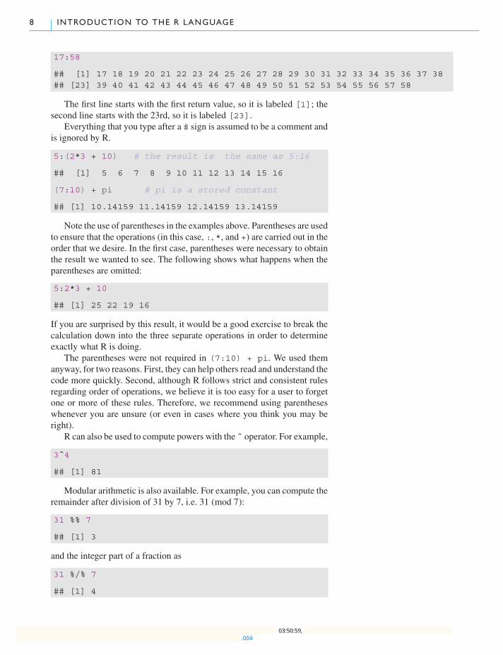
17:58
## [1] 17 18 19 20 21 22 23 24 25 26 27 28 29 30 31 32 33 34 35 36 37 38## [23] 39 40 41 42 43 44 45 46 47 48 49 50 51 52 53 54 55 56 57 58
The first line starts with the first return value, so it is labeled [1]; thesecond line starts with the 23rd, so it is labeled [23].
Everything that you type after a # sign is assumed to be a comment andis ignored by R.
5:(2*3 + 10) # the result is the same as 5:16
## [1] 5 6 7 8 9 10 11 12 13 14 15 16
(7:10) + pi # pi is a stored constant
## [1] 10.14159 11.14159 12.14159 13.14159
Note the use of parentheses in the examples above. Parentheses are usedto ensure that the operations (in this case, :, *, and +) are carried out in theorder that we desire. In the first case, parentheses were necessary to obtainthe result we wanted to see. The following shows what happens when theparentheses are omitted:
5:2*3 + 10
## [1] 25 22 19 16
If you are surprised by this result, it would be a good exercise to break thecalculation down into the three separate operations in order to determineexactly what R is doing.
The parentheses were not required in (7:10) + pi. We used themanyway, for two reasons. First, they can help others read and understand thecode more quickly. Second, although R follows strict and consistent rulesregarding order of operations, we believe it is too easy for a user to forgetone or more of these rules. Therefore, we recommend using parentheseswhenever you are unsure (or even in cases where you think you may beright).
R can also be used to compute powers with the ˆ operator. For example,
3ˆ4
## [1] 81
Modular arithmetic is also available. For example, you can compute theremainder after division of 31 by 7, i.e. 31 (mod 7):
31 %% 7
## [1] 3
and the integer part of a fraction as
31 %/% 7
## [1] 4
.004 03:50:59,
2 .1 F IRST STEPS 9
We can confirm that 31 is the sum of its remainder plus seven times theinteger part of the fraction:
7*4 + 3
## [1] 31
2.1.2 Named storageR has a workspace known as the global environment that can be used tostore the results of calculations, and many other types of objects. For afirst example, suppose we would like to store the result of the calculation1.0025ˆ30 for future use. (This might arise from a compound interestcalculation based on an interest rate of 0.25% per year and a 30-year term.)We will assign this value to an object called interest.30. To do this, wetype
interest.30 <- 1.0025ˆ30
We tell R to make the assignment using an arrow that points to the left,created with the less-than sign (<) and the hyphen (-). R also supports usingthe equals sign (=) in place of the arrow in most circumstances, but we rec-ommend using the arrow, as it makes clear that we are requesting an action(i.e. an assignment), rather than stating a relation (i.e. that interest.30is equal to 1.0025ˆ30), or making a permanent definition. Note that whenyou run this statement, no output appears: R has done what we asked, andis waiting for us to ask for something else.
You can see the results of this assignment by typing the name of ournew object at the prompt:
interest.30
## [1] 1.077783
Think of this as just another calculation: R is calculating the resultof the expression interest.30, and printing it. You can also useinterest.30 in further calculations if you wish. For example, you cancalculate the bank balance after 30 years at 0.25% annual interest, if youstart with an initial balance of $3000:
initialBalance <- 3000finalBalance <- initialBalance * interest.30finalBalance
## [1] 3233.35
Example 2.1An individual wishes to take out a loan, today, ofP at a monthly interest ratei. The loan is to be paid back in nmonthly installments of size R, beginningone month from now. The problem is to calculate R.
.004 03:50:59,
10 INTRODUCTION TO THE R LANGUAGE
Equating the present value P to the future (discounted) value of the nmonthly payments R, we have
P = R(1 + i)−1 + R(1 + i)−2 + · · · + R(1 + i)−n
or
P = Rn∑j=1
(1 + i)− j.
Summing this geometric series and simplifying, we obtain
P = R
(1 − (1 + i)−n
i
).
This is the formula for the present value of an annuity. We can find R, givenP, n, and i as
R = Pi
1 − (1 + i)−n.
In R, we define variables as follows: principal to hold the valueof P, intRate to hold the interest rate, and n to hold the number ofpayments. We will assign the resulting payment value to an object calledpayment.
Of course, we need some numerical values to work with, so wewill sup-pose that the loan amount is $1500, the interest rate is 1% and the numberof payments is 10. The required code is then
intRate <- 0.01n <- 10principal <- 1500payment <- principal * intRate / (1 - (1 + intRate)ˆ(-n))payment
## [1] 158.3731
For this particular loan, the monthly payments are $158.37.
2.1.3 Quitting RTo quit your R session, run
q()
or choose Quit RStudio... from the File menu. You will then beasked whether to save an image of the current workspace, or not, or to can-cel. The workspace image contains a record of the computations you’vedone, and may contain some saved results. Hitting the Cancel optionallows you to continue your current R session. We rarely save the currentworkspace image, but occasionally find it convenient to do so.
Note what happens if you omit the parentheses () when attempting toquit:
.004 03:50:59,

2 .2 BASIC FEATURES OF R 11
q
## function (save = "default", status = 0, runLast = TRUE)## .Internal(quit(save, status, runLast))## <bytecode: 0x7fa7ad214ad8>## <environment: namespace:base>
This has happened because q is a function that is used to tell R to quit.Typingq by itself tells R to show us the (not very pleasant-looking) contentsof the function q. By typing q(), we are telling R to call the function q. Theaction of this function is to quit R. Everything that R does is done throughcalls to functions, though sometimes those calls are hidden (as when weclick on menus), or very basic (as when we call the multiplication functionto multiply 14 times 3).
Recording your workRather than saving the workspace, we prefer to keep a record of the com-mands we entered, so that we can reproduce the workspace at a later date.The easiest way to do this is in RStudio is to enter commands in the SourcePane, and run them from there. At the end of a session, save the final scriptfor a permanent record of your work. In other systems a text editor andsome form of cut and paste serve the same purpose.
Exercises1 Calculate the remainder after dividing 31079 into 170166719.2 Calculate the interest earned after 5 years on an investment of $2000,assuming an interest rate of 3% compounded annually.
3 Using one line of R code, calculate the interest earned on an investmentof $2000, assuming an interest rate of 3% compounded annually, forterms of 1, 2, . . . , 30 years.
4 Calculate the monthly payment required for a loan of $200,000, at amonthly interest rate of 0.003, based on 300 monthly payments, start-ing in one month’s time.
5 Use R to calculate the area of a circle with radius 7 cm.6 Using one line of R code, calculate the respective areas of the circleshaving radii 3, 4, . . . , 100.
7 In the expression 48:(14*3), are the brackets really necessary? Whathappens when you type 48:14*3?
8 Do you think there is a difference between 48:14ˆ2 and 48:(14ˆ2)?Try both calculations. Using one line of code, how would you obtain thesquares of the numbers 48, 47, . . . , 14?
2.2 Basic features of R
2.2.1 FunctionsMost of the work in R is done through functions. For example, we saw thatto quit R we can type q(). This tells R to call the function named q. The
.004 03:50:59,
12 INTRODUCTION TO THE R LANGUAGE
parentheses surround the argument list, which in this case contains nothing:we just want R to quit, and do not need to tell it how.
We also saw that q is defined as
q
## function (save = "default", status = 0, runLast = TRUE)## .Internal(quit(save, status, runLast))## <bytecode: 0x7fa7ad214ad8>## <environment: namespace:base>
This shows that q is a function that has three arguments: save,status, and runLast. Each of those has a default value: "default",0, and TRUE, respectively. What happens when we execute q() is that Rcalls the q function with the arguments set to their default values.
If we want to change the default values, we specify them when we callthe function. Arguments are identified in the call by their position, or byspecifying the name explicitly. For example, both
q("no")q(save = "no")
tell R to call q with the first argument set to "no", i.e. to quit withoutsaving the workspace. If we had given two arguments without names, theywould apply to save and status. If we want to accept the defaults of theearly parameters but change later ones, we give the name when calling thefunction, e.g.
q(runLast = FALSE)
or use commas to mark the missing arguments, e.g.
q( , , FALSE)
Note that we must use = to set arguments. If we had writtenq(runLast <- FALSE) it would be interpreted quite differently fromq(runLast = FALSE). The arrow says to put the value FALSE into avariable named runLast. We then pass the result of that action (whichis the value FALSE) as the first argument of q(). Since save is the firstargument, it will act like q(save = FALSE), which is probably not whatwe wanted.
It is a good idea to use named arguments when calling a functionwhich has many arguments or when using uncommon arguments, becauseit reduces the risk of specifying the wrong argument, and makes your codeeasier to read.
2.2.2 R is case-sensitiveConsider this:
x <- 1:10MEAN(x)
## Error in eval(expr, envir, enclos): could not find function "MEAN"
.004 03:50:59,
2 .3 VECTORS IN R 13
Now try
MEAN <- meanMEAN(x)
## [1] 5.5
The function mean() is built into R. R considers MEAN to be a differentfunction, because it is case-sensitive: m is different from M.
2.2.3 Listing the objects in the workspaceThe calculations in the previous sections led to the creation of several sim-ple R objects. These objects are stored in the current R workspace. A listof all objects in the current workspace can be printed to the screen usingthe objects() function:
objects()
## [1] "finalBalance" "initialBalance" "interest.30"## [4] "intRate" "MEAN" "n"## [7] "payment" "principal" "x"
A synonym for objects() is ls().Remember that if we quit our R session without saving the workspace
image, then these objects will disappear. If we save the workspace image,then the workspace will be restored at our next R session.1 1 This will be true if we start R from
the same folder, or working directory, aswhere we ended the previous R session.Normally this will be the case, but usersare free to change the folder during asession using the menus or thesetwd() function. Type ?setwd toobtain help with this function.
2.3 Vectors in R
2.3.1 Numeric vectorsA numeric vector is a list of numbers. The c() function is used to collectthings together into a vector. We can type
c(0, 7, 8)
## [1] 0 7 8
Again, we can assign this to a named object:
x <- c(0, 7, 8) # now x is a 3-element vector
To see the contents of x, simply type
x
## [1] 0 7 8
The : symbol can be used to create sequences of increasing (or decreas-ing) values. For example,
numbers5to20 <- 5:20numbers5to20
## [1] 5 6 7 8 9 10 11 12 13 14 15 16 17 18 19 20
.004 03:50:59,

14 INTRODUCTION TO THE R LANGUAGE
Vectors can be joined together (i.e. concatenated) with the c function.For example, note what happens when we type
c(numbers5to20, x)
## [1] 5 6 7 8 9 10 11 12 13 14 15 16 17 18 19 20 0 7 8
Here is another example of the use of the c() function:
some.numbers <- c(2, 3, 5, 7, 11, 13, 17, 19, 23, 29, 31, 37, 41,43, 47, 59, 67, 71, 73, 79, 83, 89, 97, 103, 107, 109, 113, 119)
If you type this in the R console (not in the RStudio Source Pane), Rwill prompt you with a + sign for the second line of input. RStudio doesn’tadd the prompt, but it will indent the second line. In both cases you arebeing told that the first line is incomplete: you have an open parenthesiswhich must be followed by a closing parenthesis in order to complete thecommand.
We can append numbers5to20 to the end of some.numbers, andthen append the decreasing sequence from 4 to 1:
a.mess <- c(some.numbers, numbers5to20, 4:1)a.mess
## [1] 2 3 5 7 11 13 17 19 23 29 31 37 41 43 47 59## [17] 67 71 73 79 83 89 97 103 107 109 113 119 5 6 7 8## [33] 9 10 11 12 13 14 15 16 17 18 19 20 4 3 2 1
Remember that the numbers printed in square brackets give the indexof the element immediately to the right. Among other things, this helps usto identify the 22nd element of a.mess as 89: just count across from the17th element, 67.
2.3.2 Extracting elements from vectorsA nicer way to display the 22nd element of a.mess is to use square brack-ets to extract just that element:
a.mess[22]
## [1] 89
We can extract more than one element at a time. For example, the third,sixth, and seventh elements of a.mess are
a.mess[c(3, 6, 7)]
## [1] 5 13 17
To get the third through seventh elements of numbers5to20, type
numbers5to20[3:7]
## [1] 7 8 9 10 11
Negative indices can be used to avoid certain elements. For example,we can select all but the second and tenth elements of numbers5to20 asfollows:
.004 03:50:59,
2 .3 VECTORS IN R 15
numbers5to20[-c(2,10)]
## [1] 5 7 8 9 10 11 12 13 15 16 17 18 19 20
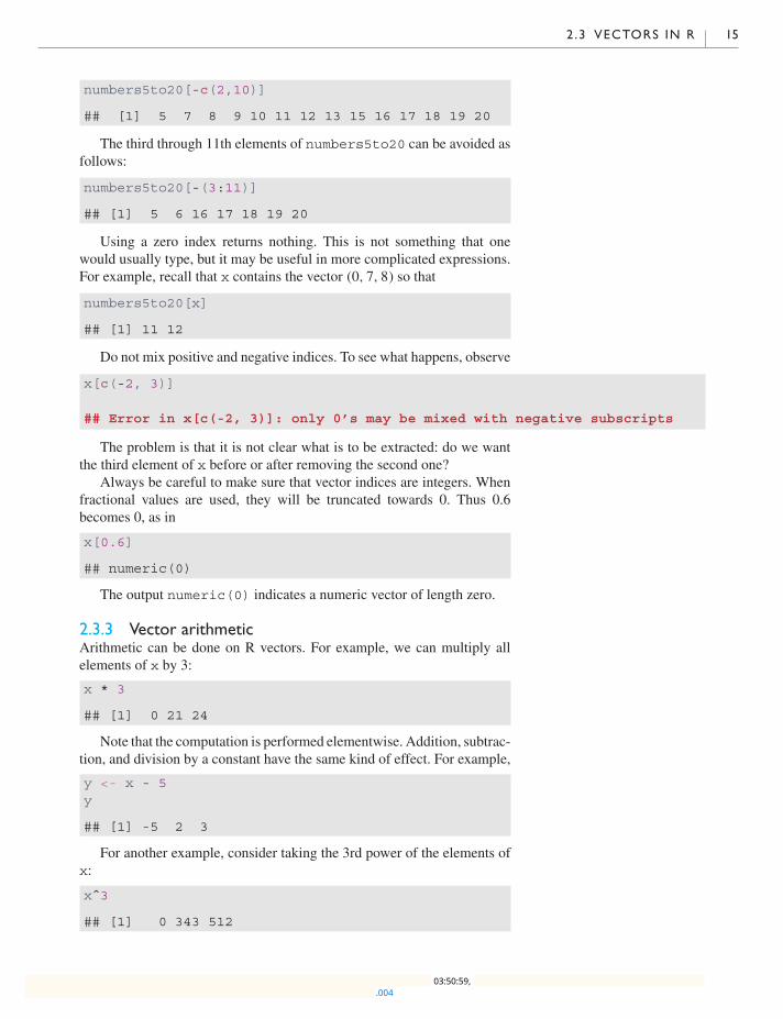
The third through 11th elements of numbers5to20 can be avoided asfollows:
numbers5to20[-(3:11)]
## [1] 5 6 16 17 18 19 20
Using a zero index returns nothing. This is not something that onewould usually type, but it may be useful in more complicated expressions.For example, recall that x contains the vector (0, 7, 8) so that
numbers5to20[x]
## [1] 11 12
Do not mix positive and negative indices. To see what happens, observe
x[c(-2, 3)]
## Error in x[c(-2, 3)]: only 0’s may be mixed with negative subscripts
The problem is that it is not clear what is to be extracted: do we wantthe third element of x before or after removing the second one?
Always be careful to make sure that vector indices are integers. Whenfractional values are used, they will be truncated towards 0. Thus 0.6becomes 0, as in
x[0.6]
## numeric(0)
The output numeric(0) indicates a numeric vector of length zero.
2.3.3 Vector arithmeticArithmetic can be done on R vectors. For example, we can multiply allelements of x by 3:
x * 3
## [1] 0 21 24
Note that the computation is performed elementwise. Addition, subtrac-tion, and division by a constant have the same kind of effect. For example,
y <- x - 5y
## [1] -5 2 3
For another example, consider taking the 3rd power of the elements ofx:
xˆ3
## [1] 0 343 512
.004 03:50:59,

16 INTRODUCTION TO THE R LANGUAGE
The above examples show how a binary arithmetic operator can beused with vectors and constants. In general, the binary operators also workelement-by-element when applied to pairs of vectors. For example, we cancompute yxii , for i = 1, 2, 3, i.e. (yx11 , yx22 , yx33 ), as follows:
yˆx
## [1] 1 128 6561
When the vectors are different lengths, the shorter one is extended byrecycling: values are repeated, starting at the beginning. For example, tosee the pattern of remainders of the numbers 1 to 10 modulo 2 and 3, weneed only give the 2:3 vector once:
c(1, 1, 2, 2, 3, 3, 4, 4, 5, 5, 6, 6, 7, 7, 8, 8, 9, 9,10, 10) %% 2:3
## [1] 1 1 0 2 1 0 0 1 1 2 0 0 1 1 0 2 1 0 0 1
R will give a warning if the length of the longer vector is not a multipleof the length of the smaller one, because that is often a symptom of an errorin the code. For example, if we wanted the remainders modulo 2, 3, and 4,this is the wrong way to do it:
c(1, 1, 2, 2, 3, 3, 4, 4, 5, 5, 6, 6, 7, 7, 8, 8, 9, 9, 10, 10) %% 2:4
## Warning in c(1, 1, 2, 2, 3, 3, 4, 4, 5, 5, 6, 6, 7, 7, 8, 8, 9, 9, 10,10)%% 2:4: longer object length is not a multiple of shorter object length
## [1] 1 1 2 0 0 3 0 1 1 1 0 2 1 1 0 0 0 1 0 1
(Do you see the error?)
2.3.4 Simple patterned vectorsWe have seen the use of the : operator for producing simple sequences ofintegers. Patterned vectors can also be produced using the seq() functionas well as the rep() function. For example, the sequence of odd numbersless than or equal to 21 can be obtained using
seq(1, 21, by = 2)
## [1] 1 3 5 7 9 11 13 15 17 19 21
Notice the use of by = 2 here. The seq() function has severaloptional parameters, including one named by. If by is not specified, thedefault value of 1 will be used.
Repeated patterns are obtained using rep(). Consider the followingexamples:
rep(3, 12) # repeat the value 3, 12 times
## [1] 3 3 3 3 3 3 3 3 3 3 3 3
rep(seq(2, 20, by = 2), 2) # repeat the pattern 2 4 ... 20, twice
## [1] 2 4 6 8 10 12 14 16 18 20 2 4 6 8 10 12 14 16 18 20
.004 03:50:59,

2 .3 VECTORS IN R 17
rep(c(1, 4), c(3, 2)) # repeat 1, 3 times and 4, twice
## [1] 1 1 1 4 4
rep(c(1, 4), each = 3) # repeat each value 3 times
## [1] 1 1 1 4 4 4
rep(1:10, rep(2, 10)) # repeat each value twice
## [1] 1 1 2 2 3 3 4 4 5 5 6 6 7 7 8 8 9 9 10 10
2.3.5 Vectors with random patternsThe sample() function allows us to simulate things like the results of therepeated tossing of a 6-sided die.
sample(1:6, size = 8, replace = TRUE) # an imaginary die is tossed 8 times
## [1] 1 5 1 5 3 1 2 1
2.3.6 Character vectorsScalars and vectors can be made up of strings of characters instead of num-bers. All elements of a vector must be of the same type. For example,
colors <- c("red", "yellow", "blue")more.colors <- c(colors, "green", "magenta", "cyan")
# this appended some new elements to colorsz <- c("red", "green", 1) # an attempt to mix data types in a vector
To see the contents of more.colors and z, simply type
more.colors
## [1] "red" "yellow" "blue" "green" "magenta" "cyan"
z # 1 has been converted to the character "1"
## [1] "red" "green" "1"
There are two basic operations you might want to perform on char-acter vectors. To take substrings, use substr(). It takes argumentssubstr(x, start, stop), where x is a vector of character strings,and start and stop say which characters to keep. For example, to printthe first two letters of each color use
substr(colors, 1, 2)
## [1] "re" "ye" "bl"
The substring() function is similar, but with slightly different def-initions of the arguments: see the help page ?substring.
The other basic operation is building up strings by concatenation. Usethe paste() function for this. For example,
paste(colors, "flowers")
## [1] "red flowers" "yellow flowers" "blue flowers"
.004 03:50:59,
18 INTRODUCTION TO THE R LANGUAGE
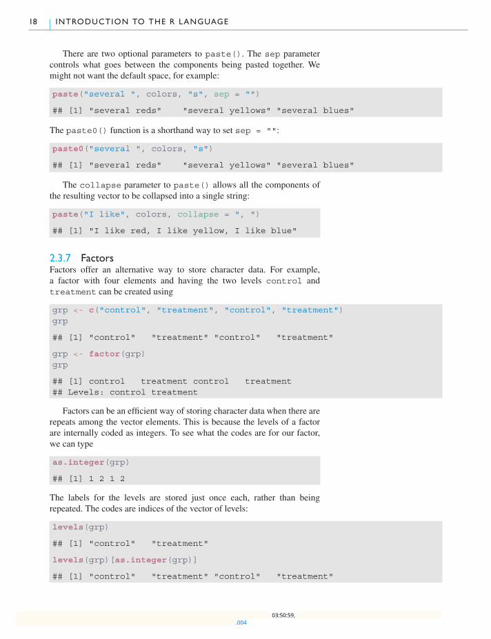
There are two optional parameters to paste(). The sep parametercontrols what goes between the components being pasted together. Wemight not want the default space, for example:
paste("several ", colors, "s", sep = "")
## [1] "several reds" "several yellows" "several blues"
The paste0() function is a shorthand way to set sep = "":
paste0("several ", colors, "s")
## [1] "several reds" "several yellows" "several blues"
The collapse parameter to paste() allows all the components ofthe resulting vector to be collapsed into a single string:
paste("I like", colors, collapse = ", ")
## [1] "I like red, I like yellow, I like blue"
2.3.7 FactorsFactors offer an alternative way to store character data. For example,a factor with four elements and having the two levels control andtreatment can be created using
grp <- c("control", "treatment", "control", "treatment")grp
## [1] "control" "treatment" "control" "treatment"
grp <- factor(grp)grp
## [1] control treatment control treatment## Levels: control treatment
Factors can be an efficient way of storing character data when there arerepeats among the vector elements. This is because the levels of a factorare internally coded as integers. To see what the codes are for our factor,we can type
as.integer(grp)
## [1] 1 2 1 2
The labels for the levels are stored just once each, rather than beingrepeated. The codes are indices of the vector of levels:
levels(grp)
## [1] "control" "treatment"
levels(grp)[as.integer(grp)]
## [1] "control" "treatment" "control" "treatment"
.004 03:50:59,
2 .3 VECTORS IN R 19
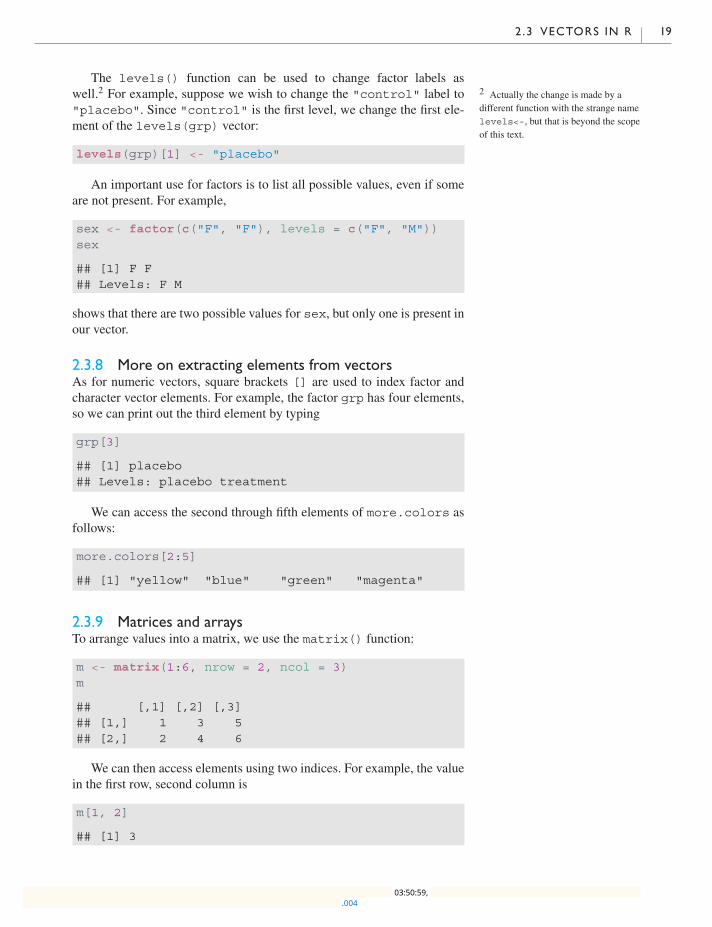
The levels() function can be used to change factor labels aswell.2 For example, suppose we wish to change the "control" label to 2 Actually the change is made by a
different function with the strange namelevels<-, but that is beyond the scopeof this text.
"placebo". Since "control" is the first level, we change the first ele-ment of the levels(grp) vector:
levels(grp)[1] <- "placebo"
An important use for factors is to list all possible values, even if someare not present. For example,
sex <- factor(c("F", "F"), levels = c("F", "M"))sex
## [1] F F## Levels: F M
shows that there are two possible values for sex, but only one is present inour vector.
2.3.8 More on extracting elements from vectorsAs for numeric vectors, square brackets [] are used to index factor andcharacter vector elements. For example, the factor grp has four elements,so we can print out the third element by typing
grp[3]
## [1] placebo## Levels: placebo treatment
We can access the second through fifth elements of more.colors asfollows:
more.colors[2:5]
## [1] "yellow" "blue" "green" "magenta"
2.3.9 Matrices and arraysTo arrange values into a matrix, we use the matrix() function:
m <- matrix(1:6, nrow = 2, ncol = 3)m
## [,1] [,2] [,3]## [1,] 1 3 5## [2,] 2 4 6
We can then access elements using two indices. For example, the valuein the first row, second column is
m[1, 2]
## [1] 3
.004 03:50:59,
20 INTRODUCTION TO THE R LANGUAGE
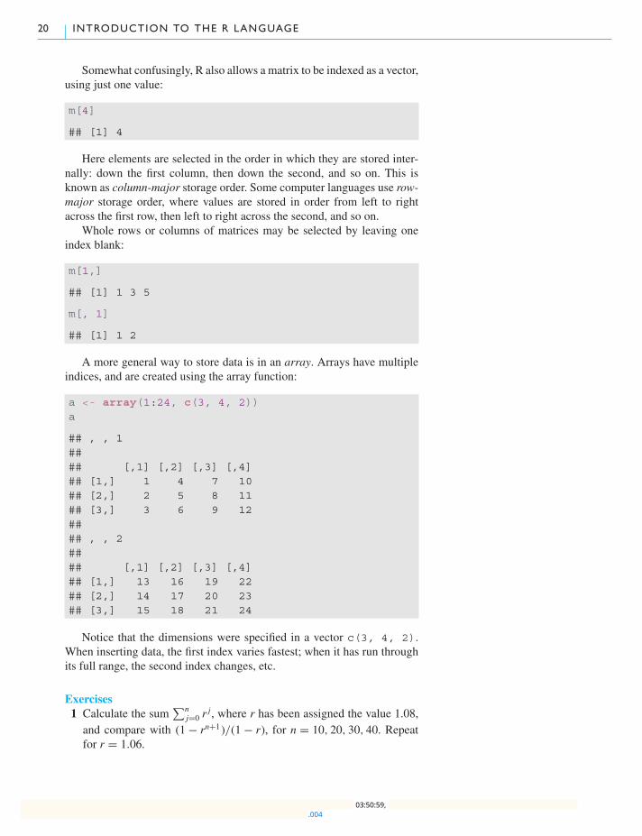
Somewhat confusingly, R also allows a matrix to be indexed as a vector,using just one value:
m[4]
## [1] 4
Here elements are selected in the order in which they are stored inter-nally: down the first column, then down the second, and so on. This isknown as column-major storage order. Some computer languages use row-major storage order, where values are stored in order from left to rightacross the first row, then left to right across the second, and so on.
Whole rows or columns of matrices may be selected by leaving oneindex blank:
m[1,]
## [1] 1 3 5
m[, 1]
## [1] 1 2
A more general way to store data is in an array. Arrays have multipleindices, and are created using the array function:
a <- array(1:24, c(3, 4, 2))a
## , , 1#### [,1] [,2] [,3] [,4]## [1,] 1 4 7 10## [2,] 2 5 8 11## [3,] 3 6 9 12#### , , 2#### [,1] [,2] [,3] [,4]## [1,] 13 16 19 22## [2,] 14 17 20 23## [3,] 15 18 21 24
Notice that the dimensions were specified in a vector c(3, 4, 2).When inserting data, the first index varies fastest; when it has run throughits full range, the second index changes, etc.
Exercises1 Calculate the sum
∑nj=0 r
j, where r has been assigned the value 1.08,and compare with (1 − rn+1)/(1 − r), for n = 10, 20, 30, 40. Repeatfor r = 1.06.
.004 03:50:59,
2 .3 VECTORS IN R 21
2 Referring to the above question, use the quick formula to compute∑nj=0 r
j, for r = 1.08, for all values of n between 1 and 100. Store the100 values in a vector.
3 Calculate the sum∑n
j=1 j and compare with n(n+ 1)/2, for n =100, 200, 400, 800.
4 Referring to the above question, use the quick formula to compute∑nj=1 j for all values of n between 1 and 100. Store the 100 values
in a vector.5 Calculate the sum
∑nj=1 j
2 and compare with n(n+ 1)(2n+ 1)/6, forn = 200, 400, 600, 800.
6 Referring to the above question, use the quick formula to compute∑nj=1 j
2 for all values of n between 1 and 100. Store the 100 valuesin a vector.
7 Calculate the sum∑N
i=1 1/i, and compare with log(N) + 0.6, forN = 500, 1000, 2000, 4000, 8000.
8 Using rep() and seq() as needed, create the vectors
0 0 0 0 0 1 1 1 1 1 2 2 2 2 2 3 3 3 3 3 4 4 4 4 4
and
1 2 3 4 5 1 2 3 4 5 1 2 3 4 5 1 2 3 4 5 1 2 3 4 5
9 Using rep() and seq() as needed, create the vector
1 2 3 4 5 2 3 4 5 6 3 4 5 6 7 4 5 6 7 8 5 6 7 8 9
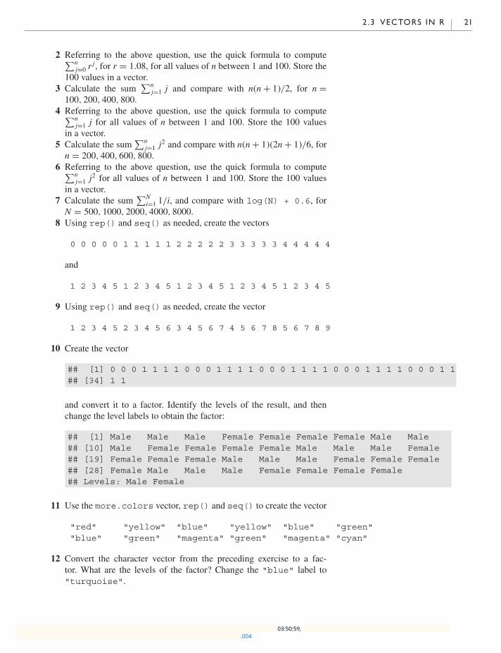
10 Create the vector
## [1] 0 0 0 1 1 1 1 0 0 0 1 1 1 1 0 0 0 1 1 1 1 0 0 0 1 1 1 1 0 0 0 1 1## [34] 1 1
and convert it to a factor. Identify the levels of the result, and thenchange the level labels to obtain the factor:
## [1] Male Male Male Female Female Female Female Male Male## [10] Male Female Female Female Female Male Male Male Female## [19] Female Female Female Male Male Male Female Female Female## [28] Female Male Male Male Female Female Female Female## Levels: Male Female
11 Use the more.colors vector, rep() and seq() to create the vector
"red" "yellow" "blue" "yellow" "blue" "green""blue" "green" "magenta" "green" "magenta" "cyan"
12 Convert the character vector from the preceding exercise to a fac-tor. What are the levels of the factor? Change the "blue" label to"turquoise".
.004 03:50:59,
22 INTRODUCTION TO THE R LANGUAGE
2.4 Data storage in R
2.4.1 Approximate storage of numbersOne important distinction in computing is between exact and approximateresults. Most of what we do in this book is aimed at approximate meth-ods. It is possible in a computer to represent any rational number exactly,but it is more common to use approximate representations: usually floatingpoint representations. These are a binary (base-two) variation on scientificnotation. For example, we might write a number to four significant dig-its in scientific notation as 6.926 × 10⁻⁴. This representation of a numbercould represent any true value between 0.00069255 and 0.00069265. Stan-dard floating point representations on computers are similar, except thata power of 2 would be used rather than a power of 10, and the fractionwould be written in binary notation. The number above would be writtenas 1.0112 × 2−11 if four binary digit precision was used. The subscript 2 inthe mantissa 1.0112 indicates that this number is shown in base 2; that is,it represents 1 × 20 + 0 × 2−1 + 1 × 2−2 + 1 × 2−3, or 1.375 in decimalnotation.
However, 6.926 × 10⁻⁴ and 1.0112 × 2−11 are not identical. Fourbinary digits give less precision than four decimal digits: a range of valuesfrom approximately 0.000641 to 0.000702 would all get the same represen-tation to four binary digit precision. In fact, 6.926 × 10⁻⁴ cannot be repre-sented exactly in binary notation in a finite number of digits. The problemis similar to trying to represent 1/3 as a decimal: 0.3333 is a close approx-imation, but is not exact. The standard precision in R is 53 binary digits,which is equivalent to about 15 or 16 decimal digits.
To illustrate, consider the fractions 5/4 and 4/5. In decimal notationthese can be represented exactly as 1.25 and 0.8, respectively. In binarynotation 5/4 is 1 + 1/4 = 1.012. How do we determine the binary repre-sentation of 4/5? It is between 0 and 1, so we’d expect something of theform 0.b1b2b3 · · · where each bi represents a “bit,” i.e. a 0 or 1 digit. Multi-plying by 2 moves all the bits left by one, i.e. 2 × 4/5 = 1.6 = b1.b2b3 · · · .Thus b1 = 1, and 0.6 = 0.b2b3 · · · .
We can now multiply by 2 again to find 2 × 0.6 = 1.2 = b2.b3 · · · , sob2 = 1. Repeating twice more yields b3 = b4 = 0. (Try it!)
At this point we’ll have the number 0.8 again, so the sequence of 4bits will repeat indefinitely: in base 2, 4/5 is 0.110011001100 · · · . SinceR stores only 53 bits, it won’t be able to store 0.8 exactly. Some roundingerror will occur in the storage.
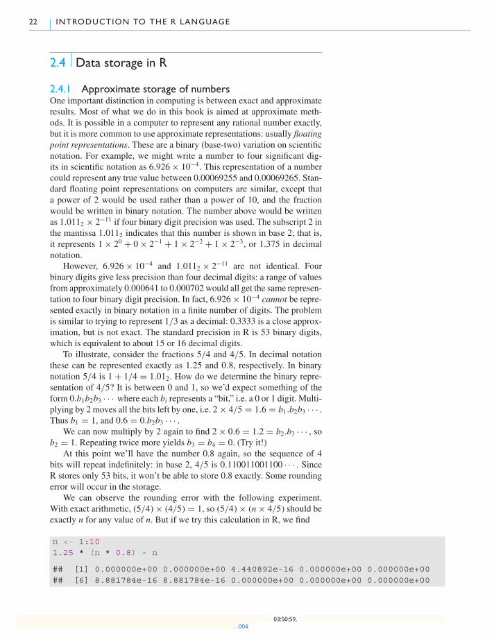
We can observe the rounding error with the following experiment.With exact arithmetic, (5/4) × (4/5) = 1, so (5/4) × (n× 4/5) should beexactly n for any value of n. But if we try this calculation in R, we find
n <- 1:101.25 * (n * 0.8) - n
## [1] 0.000000e+00 0.000000e+00 4.440892e-16 0.000000e+00 0.000000e+00## [6] 8.881784e-16 8.881784e-16 0.000000e+00 0.000000e+00 0.000000e+00
.004 03:50:59,
2 .4 DATA STORAGE IN R 23
i.e. it is equal for some values, but not equal for n = 3, 6, or 7. The errorsare very small, but non-zero.
Rounding error tends to accumulate in most calculations, so usually along series of calculations will result in larger errors than a short one. Someoperations are particularly prone to rounding error: for example, subtrac-tion of two nearly equal numbers, or (equivalently) addition of two numberswith nearly the same magnitude but opposite signs. Since the leading bitsin the binary expansions of nearly equal numbers will match, they will can-cel in subtraction, and the result will depend on what is stored in the laterbits.
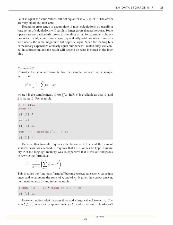
Example 2.2Consider the standard formula for the sample variance of a samplex1, . . . , xn:
s2 = 1
n− 1
n∑i=1
(xi − x)2,
where x is the sample mean, (1/n)∑xi. In R, s2 is available as var(), and
x is mean(). For example,
x <- 1:11mean(x)
## [1] 6
var(x)
## [1] 11
sum( (x - mean(x))ˆ2 ) / 10
## [1] 11
Because this formula requires calculation of x first and the sum ofsquared deviations second, it requires that all xi values be kept in mem-ory. Not too long ago memory was so expensive that it was advantageousto rewrite the formula as
s2 = 1
n− 1
(n∑i=1
x2i − nx2)
.
This is called the “one-pass formula,” because we evaluate each xi value justonce, and accumulate the sums of xi and of x2i . It gives the correct answer,both mathematically and in our example:
( sum(xˆ2) - 11 * mean(x)ˆ2 ) / 10
## [1] 11
However, notice what happens if we add a large value A to each xi. Thesum
∑ni=1 x
2i increases by approximately nA2, and so does nx2. This doesn’t
.004 03:50:59,

24 INTRODUCTION TO THE R LANGUAGE
change the variance, but it provides the conditions for a “catastrophic lossof precision” when we take the difference:
A <- 1.e10x <- 1:11 + Avar(x)
## [1] 11
( sum(xˆ2) - 11 * mean(x)ˆ2 ) / 10
## [1] 0
Since R gets the right answer, it clearly doesn’t use the one-pass for-mula, and neither should you.
2.4.2 Exact storage of numbersIn the previous section we saw that R uses floating point storage for num-bers, using a base-2 format that stores 53 bits of accuracy. It turns out thatthis format can store some fractions exactly: if the fraction can be writtenas n/2m, where n and m are integers (not too large; m can be no bigger thanabout 1000, but n can be very large), R can store it exactly. The number5/4 is in this form, but the number 4/5 is not, so only the former is storedexactly.
Floating point storage is not the only format that R uses. For wholenumbers, it can use 32 bit integer storage. In this format, numbers are storedas binary versions of the integers 0 to 232 − 1 = 4294967295. Numbersthat are bigger than 231 − 1 = 2147483647 are treated as negative valuesby subtracting 232 from them, i.e. to find the stored value for a negativenumber, add 232 to it.
Example 2.3The number 11 can be stored as the binary value of 11, i.e. 0 . . . 01011,whereas −11 can be stored as the binary value of 232 − 11 = 4294967285,which turns out to be 1 . . . 10101. If you add these two numbers together,you get 232. Using only 32 bits for storage, this is identical to 0, which iswhat we’d hope to get for 11 + (−11).
How does R decide which storage format to use? Generally, it doeswhat you (or whoever wrote the function you’re using) tell it to do. If youwant integer storage, append the letter L to the value: 11means the floatingpoint value, 11L means the integer value. Most R functions return floatingpoint values, but a few (e.g. seq(), which is used in expressions like 1:10)return integer values. Generally you don’t need to worry about this: valueswill be converted as needed.
What about 64 bit integers? Modern computers can handle 64 bits at atime, but in general, R can’t. The reason is that R expects integer values to
.004 03:50:59,
2 .4 DATA STORAGE IN R 25
be a subset of floating point values. Any 32 bit integer can be stored exactlyas a floating point value, but this is not true for all 64 bit integers.
2.4.3 Dates and timesDates and times are among the most difficult types of data to work with oncomputers. The standard calendar is very complicated: months of differentlengths, leap years every four years (with exceptions for whole centuries)and so on. When looking at dates over historical time periods, changes tothe calendar (such as the switch from the Julian calendar to the modernGregorian calendar that occurred in various countries between 1582 and1923) affect the interpretation of dates.
Times are also messy, because there is often an unstated time zone(which may change for some dates due to daylight saving time), and someyears have “leap seconds” added in order to keep standard clocks consistentwith the rotation of the earth.
There have been several attempts to deal with this in R. The basepackage has the function strptime() to convert from strings (e.g."2007-12-25" or "12/25/07") to an internal numerical representa-tion, and format() to convert back for printing. The ISOdate() andISOdatetime() functions are used when numerical values for the year,month, day, etc. are known. Other functions are available in the chronpackage. These can be difficult functions to use, and a full description isbeyond the scope of this book.
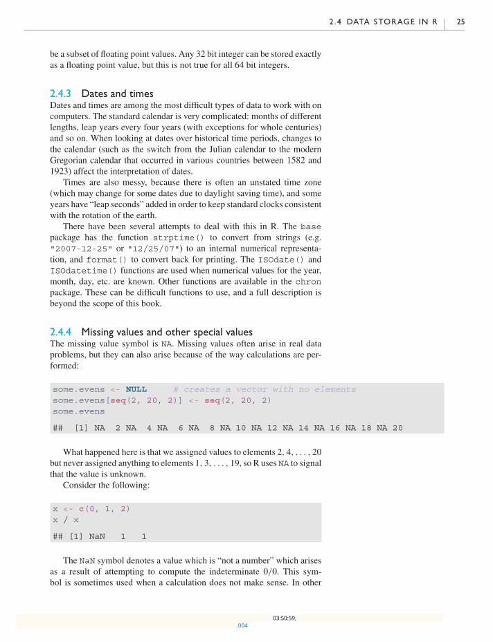
2.4.4 Missing values and other special valuesThe missing value symbol is NA. Missing values often arise in real dataproblems, but they can also arise because of the way calculations are per-formed:
some.evens <- NULL # creates a vector with no elementssome.evens[seq(2, 20, 2)] <- seq(2, 20, 2)some.evens
## [1] NA 2 NA 4 NA 6 NA 8 NA 10 NA 12 NA 14 NA 16 NA 18 NA 20
What happened here is that we assigned values to elements 2, 4, . . . , 20but never assigned anything to elements 1, 3, . . . , 19, so R uses NA to signalthat the value is unknown.
Consider the following:
x <- c(0, 1, 2)x / x
## [1] NaN 1 1
The NaN symbol denotes a value which is “not a number” which arisesas a result of attempting to compute the indeterminate 0/0. This sym-bol is sometimes used when a calculation does not make sense. In other
.004 03:50:59,

26 INTRODUCTION TO THE R LANGUAGE
cases, special values may be shown, or you may get an error or warningmessage:
1 / x
## [1] Inf 1.0 0.5
Here R has tried to evaluate 1/0 and reports the infinite result as Inf.When there may be missing values, the is.na() function should be
used to detect them. For instance,
is.na(some.evens)
## [1] TRUE FALSE TRUE FALSE TRUE FALSE TRUE FALSE TRUE FALSE TRUE## [12] FALSE TRUE FALSE TRUE FALSE TRUE FALSE TRUE FALSE
(The result is a “logical vector.” More on these in Section 2.7.) The! symbol means “not,” so we can locate the non-missing values insome.evens as follows:
!is.na(some.evens)
## [1] FALSE TRUE FALSE TRUE FALSE TRUE FALSE TRUE FALSE TRUE FALSE## [12] TRUE FALSE TRUE FALSE TRUE FALSE TRUE FALSE TRUE
We can then display the even numbers only:
some.evens[!is.na(some.evens)]
## [1] 2 4 6 8 10 12 14 16 18 20
Here we have used logical indexing, which will be further discussed inSection 2.7.2.
Exercises1 Assume 4 binary digit accuracy for the following computations.
(a) Write out the binary representation for the approximate value of6/7.
(b) Write out the binary representation for the approximate value of1/7.
(c) Add the two binary representations obtained above, and convertback to the decimal representation.
(d) Compare the result of part (c) with the result from adding the binaryrepresentations of 6 and 1, followed by division by the binary rep-resentation of 7.
2 Can you explain these two results? (Hint: see Section 2.4.1.)
x <- c(0, 7, 8)x[0.9999999999999999]
## numeric(0)
x[0.99999999999999999]
## [1] 0
.004 03:50:59,

2 .5 PACKAGES, L IBRARIES , AND REPOSITORIES 27
3 In R, evaluate the expressions
252 + k − 252,
253 + k − 253,
254 + k − 254
for the cases where k = 1, 2, 3, 4. Explain what you observe.What couldbe done to obtain results in R which are mathematically correct?
4 Explain why the following result is not a violation of Fermat’s lasttheorem:
(3987ˆ12 + 4365ˆ12)ˆ(1/12)
## [1] 4472
5 Note the output of
strptime("02/07/91", "%d/%m/%y")
and
strptime("02/07/11", "%d/%m/%y")
6 Note the output of
strptime("02/07/11", "%y/%m/%d") - strptime("02/05/11", "%y/%m/%d")
7 Note the output of
format(strptime("8/9/10", "%d/%m/%y"), "%a %b %d %Y")
2.5 Packages, libraries, and repositories
We have already mentioned several packages, i.e. base, knitr, andchron. In R, a package is a module containing functions, data, and doc-umentation. R always contains the base packages (e.g. base, stats,graphics); these contain things that everyone will use. There are alsocontributed packages (e.g. knitr and chron); these are modules writtenby others to use in R.
When you start your R session, youwill have some packages loaded andavailable for use, while others are stored on your computer in a library. Tobe sure a package is loaded, run code like
library(knitr)
To see which packages are loaded, run
search()
## [1] ".GlobalEnv" "package:knitr" "package:stats"## [4] "package:graphics" "package:grDevices" "package:utils"## [7] "package:datasets" "Autoloads" "package:base"
(Your list will likely be different from ours.) This list also indicates thesearch order: a package can contain only one function of any given name,
.004 03:50:59,

28 INTRODUCTION TO THE R LANGUAGE
but the same name may be used in another package. When you use thatfunction, R will choose it from the first package in the search list. If youwant to force a function to be chosen from a particular package, prefix thename of the function with the name of the package and ::, e.g.
stats::median(x)
Thousands of contributed packages are available, though you likelyhave only a few dozen installed on your computer. If you try to use onethat isn’t already there, you will receive an error message:
library(notInstalled)
## Error in library(notInstalled): there is no package called ’notInstalled’
Thismeans that the package doesn’t exist on your computer, but it mightbe available in a repository online. The biggest repository of R packages isknown as CRAN. To install a package fromCRAN, you can run a commandlike
install.packages("knitr")
or, within RStudio, click on the Packages tab in the Output Pane, chooseInstall, and enter the name in the resulting dialog box.
Because there are so many contributed packages, it is hard to knowwhich one to use to solve your own problems. If you can’t get help fromsomeonewithmore experience, we suggest reading the CRAN task views athttps://cloud.r-project.org/web/views. These are reviews ofavailable packages written by experts in dozens of different subject areas.
2.6 Getting help
The function q() and the other functions we have been discussing so farare examples of built-in functions. There are many functions in R which aredesigned to do all sorts of things, and we’ll discuss some more of them inthe next section. But first we want to tell you how to get help about featuresof R that you have heard about, and how to find out about features that solvenew problems.
2.6.1 Built-in help pagesThe online help facility can help you to see what a particular function issupposed to do. There are a number of ways of accessing the help facility.
If you know the name of the function that you need help with, thehelp() function is likely sufficient. It may be called with a string or func-tion name as an argument, or you can simply put a question mark (?) infront of your query. For example, for help on the q() function, type
?q
or
help(q)
.004 03:50:59,
2 .6 GETTING HELP 29
or just hit the F1 key while pointing at q in RStudio. Any of these will opena help page containing a description of the function for quitting R.
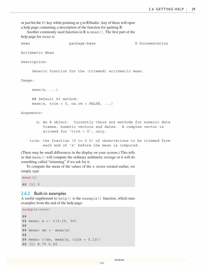
Another commonly used function in R is mean(). The first part of thehelp page for mean is
mean package:base R Documentation
Arithmetic Mean
Description:
Generic function for the (trimmed) arithmetic mean.
Usage:
mean(x, ...)
## Default S3 method:mean(x, trim = 0, na.rm = FALSE, ...)
Arguments:
x: An R object. Currently there are methods for numeric dataframes, numeric vectors and dates. A complex vector isallowed for ’trim = 0’, only.
trim: the fraction (0 to 0.5) of observations to be trimmed fromeach end of ’x’ before the mean is computed.
(There may be small differences in the display on your system.) This tellsus that mean() will compute the ordinary arithmetic average or it will dosomething called “trimming” if we ask for it.
To compute the mean of the values of the x vector created earlier, wesimply type
mean(x)
## [1] 5
2.6.2 Built-in examplesA useful supplement to help() is the example() function, which runsexamples from the end of the help page:
example(mean)
#### mean> x <- c(0:10, 50)#### mean> xm <- mean(x)#### mean> c(xm, mean(x, trim = 0.10))## [1] 8.75 5.50
.004 03:50:59,

30 INTRODUCTION TO THE R LANGUAGE
These examples show simple use of the mean() function as well ashow to use the trim argument. (When trim = 0.1, the highest 10%and lowest 10% of the data are deleted before the average is calculated.)
2.6.3 Finding help when you don’t know the function nameOne way to explore the help system is to use help.start(). This bringsup an Internet browser, such as Google Chrome or Firefox.3 The browser 3 R relies on your system having a
properly installed browser. If it doesn’thave one, you may see an error message,or possibly nothing at all.
will show you a menu of several options, including a listing of installedpackages. (The base package contains many of the routinely used func-tions; other commonly used functions are in utils or stats.) You canget to this page within RStudio by using the Help | R Helpmenu item.
Another function that is often used is help.search(), abbreviated asa double questionmark. For example, to see whether there are any functionsthat do optimization (finding minima or maxima), type
??optimization
or
help.search("optimization")
Here is the result of a such a search:
Help files with alias or concept or title matching ’optimization’ usingfuzzy matching:
lmeScale(nlme) Scale for lme Optimizationoptimization(OPM) minimize linear function with linear
constraintsconstrOptim(stats) Linearly constrained optimisationnlm(stats) Non-Linear Minimizationoptim(stats) General-purpose Optimizationoptimize(stats) One Dimensional Optimizationportfolio.optim(tseries)
Portfolio Optimization
Type ’help(FOO, package = PKG)’ to inspect entry ’FOO(PKG) TITLE’.
Your results will likely be different, depending on which R packages areinstalled on your system. We can then check for specific help on a functionlike nlm() by typing
?nlm
in the R console, or just clicking on the link in the displayed page.Web search engines such as Google can also be useful for finding help
on R. Including ‘R’ as a keyword in such a search will often bring up therelevant R help page. You may find pages describing functions that youdo not have installed, because they are in user-contributed packages. Thename of the R package that is needed is usually listed at the top of the helppage. You can usually install them by typing
install.packages("packagename")
.004 03:50:59,

2 .6 GETTING HELP 31
Histogram of islands
islands
Fre
quen
cy
0 5000 10000 15000
010
2030
40
Fig. 2.1 A histogram of theareas of the world’s 48 largestlandmasses. See Section 3.1.3 forways to improve this figure.
This will work as long as the package is still available in the CRANrepository.
Another function to note is RSiteSearch() which will do a searchin the R-help mailing list and other web resources. For example, to bringup information on the treatment of missing values in R, we can type
RSiteSearch("missing")
The sos package gives help similar to RSiteSearch(), but orga-nized differently, and triggered by a triple question mark. For example, trytyping
library(sos)???optimization
and compare the results with the ones returned by RSiteSearch().
2.6.4 Some built-in graphics functionsTwo basic plots are the histogram and the scatterplot. The codes belowwereused to produce the graphs that appear in Figures 2.1 and 2.2:
hist(islands)x <- seq(1, 10)y <- xˆ2 - 10 * xplot(x, y)
Note that the x values are plotted along the horizontal axis.Another useful plotting function is the curve() function for plotting
the graph of a univariate mathematical function on an interval. The left andright endpoints of the interval are specified by from and to arguments,respectively.
.004 03:50:59,

32 INTRODUCTION TO THE R LANGUAGE
2 4 6 8 10
−25
−20
−15
−10
−50
x
yFig. 2.2 A simple scatterplot.
0 5 10 15
−1.0
−0.5
0.0
0.5
1.0
x
sin(
x)
Fig. 2.3 Plotting the sine curve.
A simple example involves plotting the sine function on the interval[0, 6π ]:
curve(expr = sin, from = 0, to = 6 * pi)
The output is displayed in Figure 2.3. The expr parameter is eithera function (whose output is a numeric vector when the input is a numericvector) or an expression in terms ofx. An example of the latter type of usageis
curve(xˆ2 - 10 * x, from = 1, to = 10)
More information on graphics can be found in Chapter 3.
.004 03:50:59,
2 .6 GETTING HELP 33
2.6.5 Some elementary built-in functions
The sample medianThe sample median measures the middle value of a data set. If the data arex[1] ≤ x[2] ≤ · · · ≤ x[n], then the median is x[(n+ 1)/2] if n is odd, or{[x[n/2] + x[n/2 + 1]}/2 if n is even.
For example, the median of the values 10, 10, 18, 30, 32 is 18, and themedian of 40, 10, 10, 18, 30, 32 is the average of 18 and 30 (the middlevalues after putting the values into increasing order), i.e. 24.
This calculation is handled by R as follows:
median(x) # computes the median or 50th percentile of the data in x
Other summary measuresSummary statistics can be calculated for data stored in vectors. In particu-lar, try
var(x) # computes the variance of the data in xsummary(x) # computes several summary statistics on the data in xlength(x) # number of elements in xmin(x) # minimum value of xmax(x) # maximum value of xpmin(x, y) # pairwise minima of corresponding elements of x and ypmax(x, y) # pairwise maxima of x and yrange(x) # difference between maximum and minimum of data in xIQR(x) # interquartile range: difference between 1st and 3rd
# quartiles of data in x
For an example of the calculation of pairwise minima of two vectors,consider
x <- 1:5y <- 7:3pmin(x,y)
## [1] 1 2 3 4 3
Exercises1 The following are a sample of observations on incoming solar radiationat a greenhouse:
11.1 10.6 6.3 8.8 10.7 11.2 8.9 12.2
(a) Assign the data to an object called solar.radiation.(b) Find the mean, median, range, and variance of the radiation obser-
vations.(c) Add 10 to each observation of solar.radiation, and assign the
result to sr10. Find the mean, median, range, and variance of sr10.Which statistics change, and by how much?
.004 03:50:59,
34 INTRODUCTION TO THE R LANGUAGE
(d) Multiply each observation by −2, and assign the result to srm2.Find the mean, median, range, and variance of srm2. How do thestatistics change now?
(e) Plot a histogram of the solar.radiation, sr10, and srm2.2 Calculate
∑15n=1 min(2n, n3). [Hint: the min() function will give the
wrong answer.]3 Calculate
∑15n=1 max(2n, n3).
2.7 Logical vectors and relational operators
We have used the c() function to put numeric vectors together as wellas character vectors. R also supports logical vectors. These contain twodifferent elements: TRUE and FALSE, as well as NA for missing.
2.7.1 Boolean algebraTo understand how R handles TRUE and FALSE, we need to understand alittle Boolean algebra. The idea of Boolean algebra is to formalize a math-ematical approach to logic.
Logic deals with statements that are either true or false. We representeach statement by a letter or variable, e.g. A is the statement that the skyis clear, and B is the statement that it is raining. Depending on the weatherwhere you are, those two statements may both be true (there is a “sun-shower”), A may be true and B false (the usual clear day), A false and Btrue (the usual rainy day), or both may be false (a cloudy but dry day).
Boolean algebra tells us how to evaluate the truth of compound state-ments. For example, “A and B” is the statement that it is both clear andraining. This statement is true only during a sunshower. “A or B” says thatit is clear or it is raining, or both: anything but the cloudy dry day. This issometimes called an inclusive or, to distinguish it from the exclusive or “Axor B”, which says that it is either clear or raining, but not both. There isalso the “not A” statement, which says that it is not clear.
There is a very important relation between Boolean algebra and set the-ory. If we interpret A and B as sets, then we can think of “A and B” as theset of elements which are in A and are in B, i.e. the intersection A ∩ B. Sim-ilarly “A or B” can be interpreted as the set of elements that are in A or arein B, i.e. the union A ∪ B. Finally, “not A” is the complement of A, i.e. Ac.
Because there are only two possible values (true and false), we canrecord all Boolean operations in a table. On the first line of Table 2.1 welist the basic Boolean expressions, on the second line the equivalent way tocode them in R, and in the body of the table the results of the operations.
2.7.2 Logical operations in ROne of the basic types of vector in R holds logical values. For example, alogical vector may be constructed as
a <- c(TRUE, FALSE, FALSE, TRUE)
.004 03:50:59,
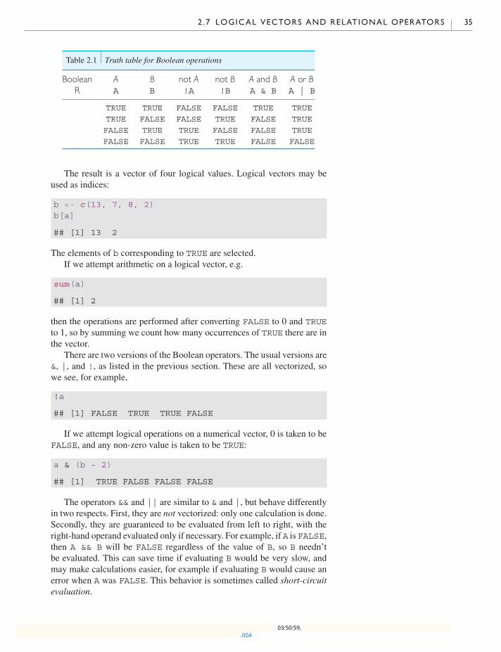
2 .7 LOGICAL VECTORS AND RELATIONAL OPERATORS 35
Table 2.1 Truth table for Boolean operations
Boolean A B not A not B A and B A or BR A B !A !B A & B A | B
TRUE TRUE FALSE FALSE TRUE TRUETRUE FALSE FALSE TRUE FALSE TRUEFALSE TRUE TRUE FALSE FALSE TRUEFALSE FALSE TRUE TRUE FALSE FALSE
The result is a vector of four logical values. Logical vectors may beused as indices:
b <- c(13, 7, 8, 2)b[a]
## [1] 13 2
The elements of b corresponding to TRUE are selected.If we attempt arithmetic on a logical vector, e.g.
sum(a)
## [1] 2
then the operations are performed after converting FALSE to 0 and TRUEto 1, so by summing we count how many occurrences of TRUE there are inthe vector.
There are two versions of the Boolean operators. The usual versions are&, |, and !, as listed in the previous section. These are all vectorized, sowe see, for example,
!a
## [1] FALSE TRUE TRUE FALSE
If we attempt logical operations on a numerical vector, 0 is taken to beFALSE, and any non-zero value is taken to be TRUE:
a & (b - 2)
## [1] TRUE FALSE FALSE FALSE
The operators && and || are similar to & and |, but behave differentlyin two respects. First, they are not vectorized: only one calculation is done.Secondly, they are guaranteed to be evaluated from left to right, with theright-hand operand evaluated only if necessary. For example, if A is FALSE,then A && B will be FALSE regardless of the value of B, so B needn’tbe evaluated. This can save time if evaluating B would be very slow, andmay make calculations easier, for example if evaluating B would cause anerror when A was FALSE. This behavior is sometimes called short-circuitevaluation.
.004 03:50:59,
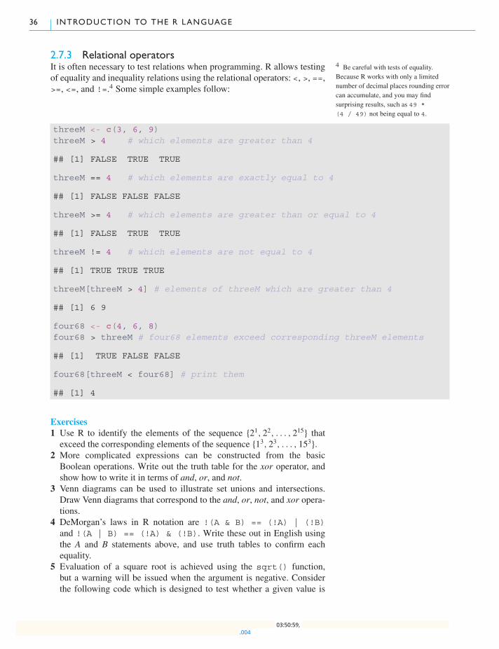
36 INTRODUCTION TO THE R LANGUAGE
2.7.3 Relational operatorsIt is often necessary to test relations when programming. R allows testingof equality and inequality relations using the relational operators: <, >, ==,>=, <=, and !=.4 Some simple examples follow:
4 Be careful with tests of equality.Because R works with only a limitednumber of decimal places rounding errorcan accumulate, and you may findsurprising results, such as 49 *
(4 / 49) not being equal to 4.
threeM <- c(3, 6, 9)threeM > 4 # which elements are greater than 4
## [1] FALSE TRUE TRUE
threeM == 4 # which elements are exactly equal to 4
## [1] FALSE FALSE FALSE
threeM >= 4 # which elements are greater than or equal to 4
## [1] FALSE TRUE TRUE
threeM != 4 # which elements are not equal to 4
## [1] TRUE TRUE TRUE
threeM[threeM > 4] # elements of threeM which are greater than 4
## [1] 6 9
four68 <- c(4, 6, 8)four68 > threeM # four68 elements exceed corresponding threeM elements
## [1] TRUE FALSE FALSE
four68[threeM < four68] # print them
## [1] 4
Exercises1 Use R to identify the elements of the sequence {21, 22, . . . , 215} that
exceed the corresponding elements of the sequence {13, 23, . . . , 153}.2 More complicated expressions can be constructed from the basicBoolean operations. Write out the truth table for the xor operator, andshow how to write it in terms of and, or, and not.
3 Venn diagrams can be used to illustrate set unions and intersections.Draw Venn diagrams that correspond to the and, or, not, and xor opera-tions.
4 DeMorgan’s laws in R notation are !(A & B) == (!A) | (!B)and !(A | B) == (!A) & (!B). Write these out in English usingthe A and B statements above, and use truth tables to confirm eachequality.
5 Evaluation of a square root is achieved using the sqrt() function,but a warning will be issued when the argument is negative. Considerthe following code which is designed to test whether a given value is
.004 03:50:59,
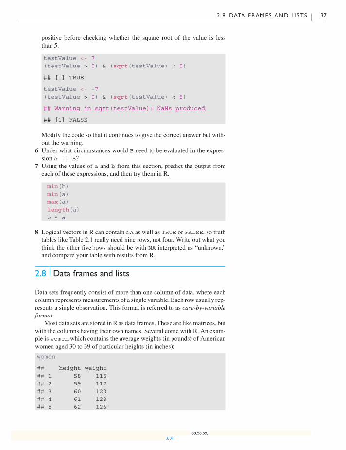
2 .8 DATA FRAMES AND LISTS 37
positive before checking whether the square root of the value is lessthan 5.
testValue <- 7(testValue > 0) & (sqrt(testValue) < 5)
## [1] TRUE
testValue <- -7(testValue > 0) & (sqrt(testValue) < 5)
## Warning in sqrt(testValue): NaNs produced
## [1] FALSE
Modify the code so that it continues to give the correct answer but with-out the warning.
6 Under what circumstances would B need to be evaluated in the expres-sion A || B?
7 Using the values of a and b from this section, predict the output fromeach of these expressions, and then try them in R.
min(b)min(a)max(a)length(a)b * a
8 Logical vectors in R can contain NA as well as TRUE or FALSE, so truthtables like Table 2.1 really need nine rows, not four. Write out what youthink the other five rows should be with NA interpreted as “unknown,”and compare your table with results from R.
2.8 Data frames and lists
Data sets frequently consist of more than one column of data, where eachcolumn representsmeasurements of a single variable. Each row usually rep-resents a single observation. This format is referred to as case-by-variableformat.
Most data sets are stored in R as data frames. These are likematrices, butwith the columns having their own names. Several come with R. An exam-ple is women which contains the average weights (in pounds) of Americanwomen aged 30 to 39 of particular heights (in inches):
women
## height weight## 1 58 115## 2 59 117## 3 60 120## 4 61 123## 5 62 126
.004 03:50:59,
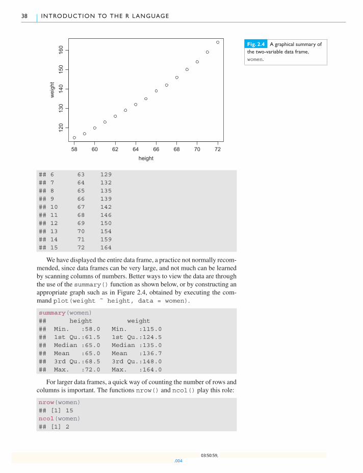
38 INTRODUCTION TO THE R LANGUAGE
58 60 62 64 66 68 70 72
120
130
140
150
160
height
wei
ght
Fig. 2.4 A graphical summary ofthe two-variable data frame,women.
## 6 63 129## 7 64 132## 8 65 135## 9 66 139## 10 67 142## 11 68 146## 12 69 150## 13 70 154## 14 71 159## 15 72 164
We have displayed the entire data frame, a practice not normally recom-mended, since data frames can be very large, and not much can be learnedby scanning columns of numbers. Better ways to view the data are throughthe use of the summary() function as shown below, or by constructing anappropriate graph such as in Figure 2.4, obtained by executing the com-mand plot(weight ˜ height, data = women).
summary(women)## height weight## Min. :58.0 Min. :115.0## 1st Qu.:61.5 1st Qu.:124.5## Median :65.0 Median :135.0## Mean :65.0 Mean :136.7## 3rd Qu.:68.5 3rd Qu.:148.0## Max. :72.0 Max. :164.0
For larger data frames, a quick way of counting the number of rows andcolumns is important. The functions nrow() and ncol() play this role:
nrow(women)## [1] 15ncol(women)## [1] 2
.004 03:50:59,

2 .8 DATA FRAMES AND LISTS 39
We can get both at once using dim() (for dimension):
dim(women)
## [1] 15 2
and can get summary information using str() (for structure):
str(women)
## ’data.frame’: 15 obs. of 2 variables:## $ height: num 58 59 60 61 62 63 64 65 66 67 ...## $ weight: num 115 117 120 123 126 129 132 135 139 142 ...
In fact, str() works with almost any R object, and is often a quick wayto find out what you are working with.
2.8.1 Extracting data frame elements and subsetsWe can extract elements from data frames using similar syntax to what wasused with matrices. Consider the following examples:
women[7, 2]
## [1] 132
women[3, ]
## height weight## 3 60 120
women[4:7, 1]
## [1] 61 62 63 64
Data frame columns can also be addressed using their names using the$ operator. For example, the weight column can be extracted as follows:
women$weight
## [1] 115 117 120 123 126 129 132 135 139 142 146 150 154 159 164
Thus, we can extract all heights for which the weights exceed 140 using
women$height[women$weight > 140]
## [1] 67 68 69 70 71 72
The with() function allows us to access columns of a data framedirectly without using the $. For example, we can divide the weights bythe heights in the women data frame using
with(women, weight/height)
## [1] 1.982759 1.983051 2.000000 2.016393 2.032258 2.047619 2.062500## [8] 2.076923 2.106061 2.119403 2.147059 2.173913 2.200000 2.239437## [15] 2.277778
See help(with) for more information.
.004 03:50:59,

40 INTRODUCTION TO THE R LANGUAGE
2.8.2 Taking random samples from populationsThe sample() function can be used to take samples (with or withoutreplacement) from larger finite populations. Suppose, for example, that wehave a data frame called fluSurvey consisting of 15000 entries, and wewould like to randomly select 8 entries (without replacement) for detailedstudy. If the entries have been enumerated (say, by the use of an ID index)from 1 through 15000, we could select the 8 numbers with
sampleID <- sample(1:15000, size = 8, replace = FALSE)sampleID
## [1] 7940 13609 11786 87 3850 5947 373 4767
The above numbers have been chosen randomly (or at least approxi-mately so), and the random rows of fluSurvey, a supposedly existing dataframe, can now be extracted with
fluSample <- fluSurvey[sampleID,]
The result is a new data frame consisting of 8 rows and the same numberof columns as fluSurvey.
2.8.3 Constructing data framesUse the data.frame() function to construct data frames from vectorsthat already exist in your workspace:
xy <- data.frame(x, y)xy
## x y## 1 1 7## 2 2 6## 3 3 5## 4 4 4## 5 5 3
For another example, consider
xynew <- data.frame(x, y, new = 10:1)
2.8.4 Data frames can have non-numeric columnsColumns of data frames can be of different types. For example, the built-in data frame chickwts has a numeric column and a factor. Again, thesummary() function provides a quick peek at this data set:
summary(chickwts)
## weight feed## Min. :108.0 casein :12## 1st Qu.:204.5 horsebean:10## Median :258.0 linseed :12## Mean :261.3 meatmeal :11## 3rd Qu.:323.5 soybean :14## Max. :423.0 sunflower:12
.004 03:50:59,
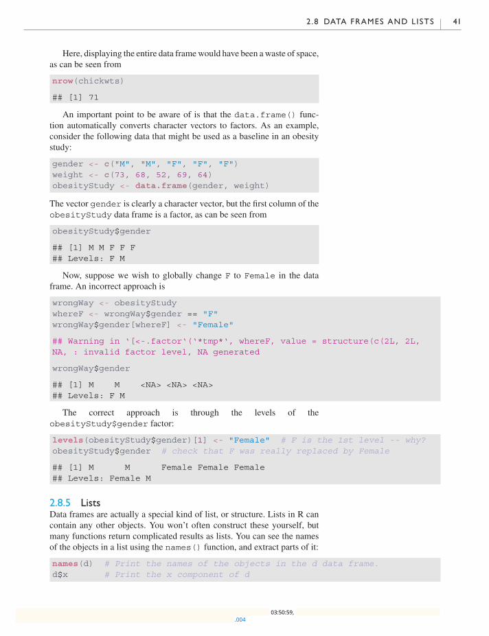
2 .8 DATA FRAMES AND LISTS 41
Here, displaying the entire data framewould have been awaste of space,as can be seen from
nrow(chickwts)
## [1] 71
An important point to be aware of is that the data.frame() func-tion automatically converts character vectors to factors. As an example,consider the following data that might be used as a baseline in an obesitystudy:
gender <- c("M", "M", "F", "F", "F")weight <- c(73, 68, 52, 69, 64)obesityStudy <- data.frame(gender, weight)
The vector gender is clearly a character vector, but the first column of theobesityStudy data frame is a factor, as can be seen from
obesityStudy$gender
## [1] M M F F F## Levels: F M
Now, suppose we wish to globally change F to Female in the dataframe. An incorrect approach is
wrongWay <- obesityStudywhereF <- wrongWay$gender == "F"wrongWay$gender[whereF] <- "Female"
## Warning in ‘[<-.factor‘(‘*tmp*‘, whereF, value = structure(c(2L, 2L,NA, : invalid factor level, NA generated
wrongWay$gender
## [1] M M <NA> <NA> <NA>## Levels: F M
The correct approach is through the levels of theobesityStudy$gender factor:
levels(obesityStudy$gender)[1] <- "Female" # F is the 1st level -- why?obesityStudy$gender # check that F was really replaced by Female
## [1] M M Female Female Female## Levels: Female M
2.8.5 ListsData frames are actually a special kind of list, or structure. Lists in R cancontain any other objects. You won’t often construct these yourself, butmany functions return complicated results as lists. You can see the namesof the objects in a list using the names() function, and extract parts of it:
names(d) # Print the names of the objects in the d data frame.d$x # Print the x component of d
.004 03:50:59,

42 INTRODUCTION TO THE R LANGUAGE
The list() function is one way of organizing multiple pieces of out-put from functions. For example,
x <- c(3, 2, 3)y <- c(7, 7)z <- list(x = x, y = y)z
## $x## [1] 3 2 3#### $y## [1] 7 7
There are several functions which make working with lists easy. Two ofthem are lapply() and vapply(). The lapply() function “applies”another function to every element of a list and returns the results in a newlist; for example,
lapply(z, mean)
## $x## [1] 2.666667#### $y## [1] 7
In a case like this, it might be more convenient to have the results in avector; the vapply() function does that. It takes a third argument to tellR what kind of result to expect from the function. In this case each resultof mean should be a number, so we could use
vapply(z, mean, 1)
## x y## 2.666667 7.000000
where the 1 just serves as an example of the type of output expected. Ifmean() had returned a different kind of result, vapply() would havegiven an error. If we expect more than a single value, the results will beorganized into a matrix, e.g.
vapply(z, summary, numeric(6))
## x y## Min. 2.000 7## 1st Qu. 2.500 7## Median 3.000 7## Mean 2.667 7## 3rd Qu. 3.000 7## Max. 3.000 7
Exercises1 Consider the built-in data frame Formaldehyde.
(a) Extract the elements of the third row of this data frame.(b) Extract the elements of the carb (carbohydrate) column.
.004 03:50:59,

2 .9 DATA INPUT AND OUTPUT 43
(c) Use the plot() function to identify the relation between optden(optical density) and carb.
2 Consider the built-in USArrests data frame.(a) Determine the number of rows and columns for this data frame.(b) Calculate the median of each column of this data frame.(c) Find the average per capita murder rate (Murder) in regions where
the percentage of the population living in urban areas (UrbanPop)exceeds 77%. Compare this with the average per capita murder ratewhere urban area population is less than 50%.
(d) Construct a new data frame consisting of a random sample of 12 ofthe records of the USArrests data frame, where the records havebeen sampled without replacement.
2.9 Data input and output
When in an R session, it is possible to read and write data to files outside ofR, for example on your computer’s hard drive. Before we can discuss someof the many ways of doing this, it is important to know where the data arecoming from or going to.
2.9.1 Changing directoriesIn the RStudio Files tab of the output pane you can navigate tothe directory where you want to work, and choose Set As WorkingDirectory from the More menu item. Alternatively you can run the Rfunction setwd(). For example, to work with data in the foldermydata onthe C:drive, run
setwd("c:/mydata") # or setwd("c:\\mydata")
After running this command, all data input and output will default to themydata folder in the C:drive.5 5 If you are accustomed to folder names
in Windows, you might have expectedthis to be written as "c:\mydata".However, R treats the backslashcharacter “\” as a special “escape”character, which modifies theinterpretation of the next character. Ifyou really want a backslash, you need todouble it: the first backslash tells thesecond backslash not to be an escape.Because other systems use a forwardslash “/” in their folder names, andbecause doubling the backslash istedious in Windows, R accepts eitherform.
2.9.2 dump() and source()Suppose you have constructed an R object called usefuldata. In orderto save this object for a future session, type
dump("usefuldata", "useful.R")
This stores the command necessary to create the vector usefuldata intothe file useful.R on your computer’s hard drive. The choice of filename isup to you, as long as it conforms to the usual requirements for filenameson your computer.
To retrieve the vector in a future session, type
source("useful.R")
This reads and executes the command in useful.R, resulting in the cre-ation of the usefuldata object in your global environment. If there wasan object of the same name there before, it will be replaced.
.004 03:50:59,
44 INTRODUCTION TO THE R LANGUAGE
To save all of the objects that you have created during a session, type
dump(list = objects(), "all.R")
This produces a file called all.R on your computer’s hard drive. Usingsource("all.R") at a later time will allow you to retrieve all of theseobjects.
Example 2.4To save existing objects humidity, temp, and rain to a file calledweather.R on your hard drive, type
dump(c("humidity", "temp", "rain"), "weather.R")
Exercises1 Use a text editor to create a file consisting of the line
randomdata <- c(64, 38, 97, 88, 24, 14, 104, 83)
Save it to a file called randomdata.2 Source the file randomdata into R and confirm that the randomdatavector was created.
3 Create a vector called numbers which contains
3 5 8 10 12
Dump numbers to a file called numbers.R and delete numbers usingthe rm() function. Using ls(), confirm that numbers has beendeleted. Now, use the source command to retrieve the vector numbers.
2.9.3 Redirecting R outputBy default, R directs the output of most of its functions to the screen. Outputcan be directed to a file with the sink() function.
Example 2.5Consider the greenhouse data in solar.radiation. The commandmean(solar.radiation) prints the mean of the data to the screen. Toprint this output to a file called solarmean.txt instead, run
sink("solarmean.txt") # Create a file solarmean.txt for outputmean(solar.radiation) # Write mean value to solarmean.txt
All subsequent output will be printed to the file solarmean.txt until thecommand
sink() # Close solarmean.txt; print new output to screen
is invoked. This returns subsequent output to the screen.
.004 03:50:59,
2 .9 DATA INPUT AND OUTPUT 45
2.9.4 Saving and retrieving image filesThe vectors and other objects created during an R session are stored in theworkspace known as the global environment. When ending an R session,we have the option of saving the workspace in a file called a workspaceimage. If we choose to do so, a file called by default .RData is created in thecurrent working directory (folder) which contains the information neededto reconstruct this workspace. In Windows, the workspace image will beautomatically loaded if R is started by clicking on the icon representing thefile .RData, or if the .RData file is saved in the directory from which R isstarted. If R is started in another directory, the load() function may beused to load the workspace image.
It is also possible to save workspace images without quitting. For exam-ple, we could save all current workspace image information to a file calledtemp.RData by typing
save.image("temp.RData")
Again, we can begin an R session with that workspace image,by clicking on the icon for temp.RData. Alternatively, we can typeload("temp.RData") after entering an R session. Objects that werealready in the current workspace image will remain, unless they have thesame name as objects in the workspace image associated with temp.RData.In the latter case, the current objects will be overwritten and lost.
2.9.5 The read.table functionThe following data set consists of four observations on the three variablesx, y, and z:
x y z61 13 4
175 21 18111 24 14124 23 18
If such a data set is stored in a file called pretend.dat in the directorymyfiles on the C: drive, then it can be read into an R data frame. This canbe accomplished by typing
pretend.df <- read.table("c:/myfiles/pretend.dat", header = TRUE)
The result is a data frame called pretend.df to which the usual dataframe operations apply, such as pretend.df$x which would extract thefirst column of data.
Comma-separated version (csv) files can be read in using thesep = "," argument in read.table().
In practice, it is unusual for data files to be as clean as pretend.df.More often, data files are littered with blanks and other oddities. For exam-ple, suppose file1.txt has the following contents:
x, y, z3, , 451, 48, 2323, 33, 111
.004 03:50:59,

46 INTRODUCTION TO THE R LANGUAGE
Reading in such a file with blank missing values is accomplished using
dataset1 <-read.table("file1.txt", header = TRUE, sep = ",", na.string = " ")
In the above code, the na.string parameter replaces blank valueswith the NA missing value symbol. The contents of the data frame are
> dataset1x y z
1 3 NA 42 51 48 233 23 33 111
For another example, suppose the fields in file2.txt are separated by tabsand the contents, when viewed in a text editor that displays tabs as <tab>appear as follows:
x<tab>y<tab>z33<tab>223<tab>32<tab>88<tab>23<tab><tab>7
Reading in such a file with columns separated by tabs with blank missingvalues can be carried out using
dataset2 <-read.table("file2.txt", header = TRUE, sep = "\t", na.string = " ")
The outcome of this is to produce a data frame with the followingcontents:
dataset2
## x y z## 1 33 223 NA## 2 32 88 2## 3 3 NA 7
Exercises1 Display the row 1, column 3 element of pretend.df.2 Use two different commands to display the y column of pretend.df.
Chapter exercises1 Calculate 112, 1112 and 11112, and note the pattern in the sequence of
results. Now, compute 111111112. In order to see all of the digits, tryoptions(digits = 18) before carrying out the calculation. Finally,calculate 1111111112. Did you obtain the correct answer? Why or whynot?
2 How might you correct the following statement: “There are 10 kinds ofpeople: those that understand binary and those that do not.”
3 Consider the built-in data frame chickwts.(a) Create a subset of the data frame called chickwts300pwhich con-
tains all observations for which the weight exceeds 300.
.004 03:50:59,
CHAPTER EXERCISES 47
(b) Create another subset called chickwtsLinseed which containsall observations for which the chicks were fed linseed.
(c) Calculate the average weight of the chicks which were fed linseed.(d) Calculate the average weight of the chicks which were not fed
linseed.4 Consider the built-in data frame cars.(a) Consult the help page to determine the number of observations in
the dataset as well as the number of variables. Also, what are thenames of the variables?
(b) Find the mean stopping distance for all observations for which thespeed was 20 miles per hour.
(c) Construct a scatterplot relating stopping distance to speed. Whatkind of relationship do you observe?
5 Assign the data set in rnf6080.dat6 to a data frame called rain.df. Use the 6 This data set is available atwww.statprogr.science/data/
rnf6080.dat.header = FALSE option.(a) Display the row 2, column 4 element of rain.df.(b) What are the names of the columns of rain.df?(c) Display the contents of the 2nd row of the rain.df dataset.(d) Use the following command to re-label the columns of this data
frame:
names(rain.df) <- c("year", "month", "day", seq(0, 23))
(e) Create a new column called dailywhich is the sum of the 24 hourlycolumns.
(f) Plot a histogram of the daily rainfall amounts.6 Plot the graph of the function
f (x) ={3x+ 2, x ≤ 32x− 0.5x2, x > 3
on the interval [0, 6].7 The goal of this exercise is for you to use artificial data to see what theadvantages of factors are over numeric and character vectors.(a) Use the sample() function to construct a vector called dieRolls
which simulates the results of 1000000 tosses of a six-sided die.(b) Convert dieRolls to a factor called dieRollsFactor. Change
the levels of the factor using the code
levels(dieRollsFactor)<- c("One", "Two", "Three", "Four", "Five","Six")
(c) Create a character version of the vector using
dieRollsChar <- as.character(dieRollsFactor)
(d) Apply the table() function to each of dieRolls,dieRollsFactor, and dieRollsChar, and compare theresults as well as how the information in each of the data sets isdisplayed.
.004 03:50:59,

48 INTRODUCTION TO THE R LANGUAGE
(e) Run the code
system.time(table(dieRolls))system.time(table(dieRollsFactor))system.time(table(dieRollsChar))
to compare the length of time required to construct the three tables,using each data type. Which table was produced most quickly?Which was the slowest?
(f) Run the code
dump("dieRolls", "dieRolls.R")dump("dieRollsFactor", "dieRollsFactor.R")dump("dieRollsChar", "dieRollsChar.R")
Investigate the properties of the files dieRolls.R, dieRollsFactor.R,and dieRollsChar.R; which one requires the smallest amount ofmemory? Which file takes the most memory?
8 What happens when the following code is run?
gender <- c("M", "M", "F", "F", "F")whereF <- (gender == "F")gender[whereF] <- "Female"
9 Construct the data frame charnum in the following way:
char <- c("2", "1", "0")num <- 0:2charnum <- data.frame(char, num)
The as.numeric() function coerces character data to becomenumeric (when possible). Apply as.numeric() to char and tocharnum$char. Can you explain why there is a difference in theresults?
.004 03:50:59,

3
Programming statistical graphics
Users of statistical computing need to produce graphs of their data andthe results of their computations. In this chapter we start with a generaloverview of how this is done in R, and learn how to draw some basic plots.We then discuss some of the issues involved in choosing a style of plot todraw: it is not always an easy choice, and there are plenty of bad examplesin the world to lead us astray. Finally, we will go into some detail abouthow to customize graphs in R.
There are several different graphics systems in R. The oldest one is mostdirectly comparable to the original S graphics, and is now known as basegraphics. You can think of base graphics as analogous to drawing with inkon paper. You build up a picture by drawing fixed things on it, and oncesomething is drawn, it is permanent, though you might be able to coverit with something else, or move to a clean sheet of paper. Since the verybeginning, base graphics has been designed to allow easy production ofgood quality scientific plots. In this chapter we will concentrate on basegraphics.
The grid package provides the basis for a newer graphics system. Italso has facilities to produce good quality graphics, but the programmer hasaccess to the individual pieces of a graph, and can modify them: a graphis more like a physical model being built and displayed, rather than justdrawn. The lattice and ggplot2 packages provide functions for high-level plots based on grid graphics.
Both base and grid graphics are designed to be “device independent.”Directions are given regarding where to draw and these drawing commandswork on any device. The actual look of a graph will vary slightly fromone device to another (e.g. on paper versus in a window on your screen),because of their different capabilities.
There are other more exotic graphics systems available in R as well,providing interactive graphics, 3D displays, etc. Some of these will be men-tioned briefly in Section 3.4.
.00513:57:15,
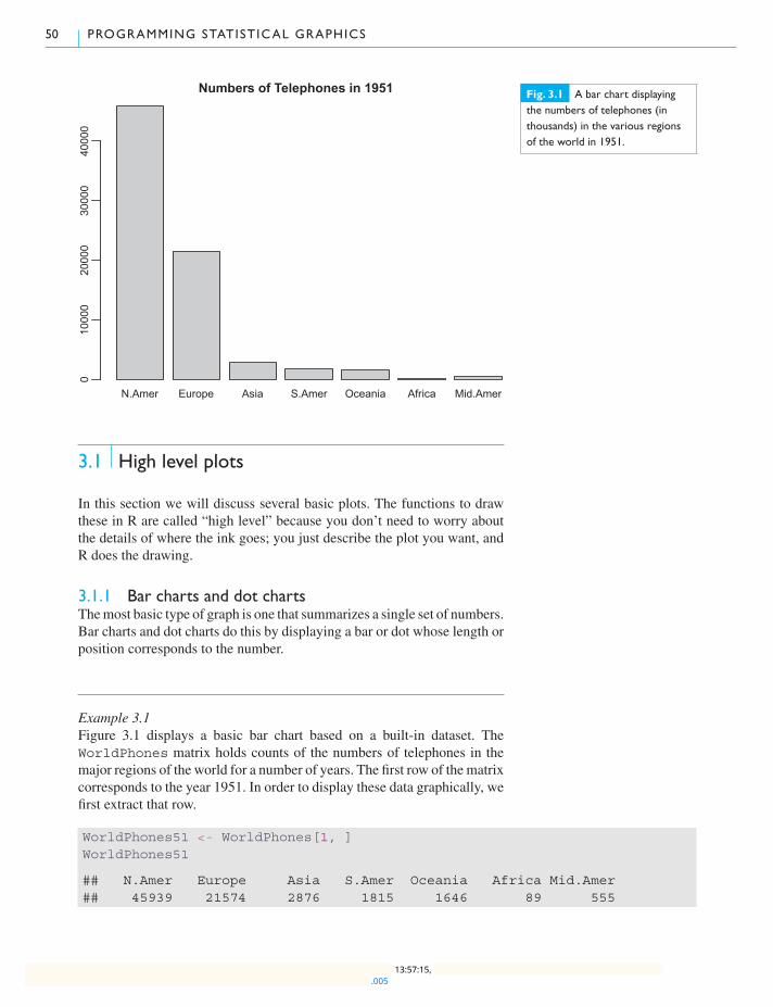
50 PROGRAMMING STATISTICAL GRAPHICS
N.Amer Europe Asia S.Amer Oceania Africa Mid.Amer
Numbers of Telephones in 19510
1000
020
000
3000
040
000
Fig. 3.1 A bar chart displayingthe numbers of telephones (inthousands) in the various regionsof the world in 1951.
3.1 High level plots
In this section we will discuss several basic plots. The functions to drawthese in R are called “high level” because you don’t need to worry aboutthe details of where the ink goes; you just describe the plot you want, andR does the drawing.
3.1.1 Bar charts and dot chartsThemost basic type of graph is one that summarizes a single set of numbers.Bar charts and dot charts do this by displaying a bar or dot whose length orposition corresponds to the number.
Example 3.1Figure 3.1 displays a basic bar chart based on a built-in dataset. TheWorldPhones matrix holds counts of the numbers of telephones in themajor regions of the world for a number of years. The first row of the matrixcorresponds to the year 1951. In order to display these data graphically, wefirst extract that row.
WorldPhones51 <- WorldPhones[1, ]WorldPhones51
## N.Amer Europe Asia S.Amer Oceania Africa Mid.Amer## 45939 21574 2876 1815 1646 89 555
.00513:57:15,

3 .1 HIGH LEVEL PLOTS 51
N.Amer
Europe
Asia
S.Amer
Oceania
Africa
Mid.Amer
●
●
●
●
●
●
●
0 10000 20000 30000 40000Numbers of Phones ('000s)
Fig. 3.2 World telephone countsin 1951 displayed as a dot chart.
We could plot the bar chart using the barplot() function as
barplot(WorldPhones51)
(try it!), but the plot that results needs some minor changes: we’d like todisplay a title at the top, and we’d like to shrink the size of the labels on theaxes. We can do that with the following code.
barplot(WorldPhones51, cex.names = 0.75, cex.axis = 0.75,main = "Numbers of Telephones in 1951")
Understanding the codeThe cex.names = 0.75 argument reduced the size of the region namesto 0.75 of their former size, and the cex.axis = 0.75 argument reducedthe labels on the vertical axis by the same amount. The main argument setsthe main title for the plot.
An alternative way to plot the same kind of data is in a dot chart(Figure 3.2):
dotchart(WorldPhones51, xlab = "Numbers of Phones (’000s)")
The values are shown by the horizontal positions of the dots.
Data sets having more complexity can also be displayed using thesegraphics functions. The barplot() function has a number of optionswhich allow for side-by-side or stacked styles of displays, legends can beincluded using the legend argument, and so on.
.00513:57:15,

52 PROGRAMMING STATISTICAL GRAPHICS
Rural Male Rural Female Urban Male Urban Female
50−5455−5960−6465−6970−74
Death rates in Virginia
Dea
ths
per 1
000
020
4060
80
Fig. 3.3 An example of acomplex bar chart.
Example 3.2The VADeaths dataset in R contains death rates (number of deaths per1000 population per year) in various subpopulations within the state ofVirginia in 1940.
VADeaths
## Rural Male Rural Female Urban Male Urban Female## 50-54 11.7 8.7 15.4 8.4## 55-59 18.1 11.7 24.3 13.6## 60-64 26.9 20.3 37.0 19.3## 65-69 41.0 30.9 54.6 35.1## 70-74 66.0 54.3 71.1 50.0
This data set may be displayed as a sequence of bar charts, one for eachsubgroup (Figure 3.3):
barplot(VADeaths, beside = TRUE, legend = TRUE, ylim = c(0, 90),ylab = "Deaths per 1000",main = "Death rates in Virginia")
Understanding the codeThe bars correspond to each number in the matrix. The beside = TRUEargument causes the values in each column to be plotted side-by-side;legend = TRUE causes the legend in the top right to be added. Theylim = c(0, 90) argument modifies the vertical scale of the graph tomake room for the legend. (We will describe other ways to place the legendin Section 3.3.) Finally, main = "Death rates in Virginia" setsthe main title for the plot.
.00513:57:15,
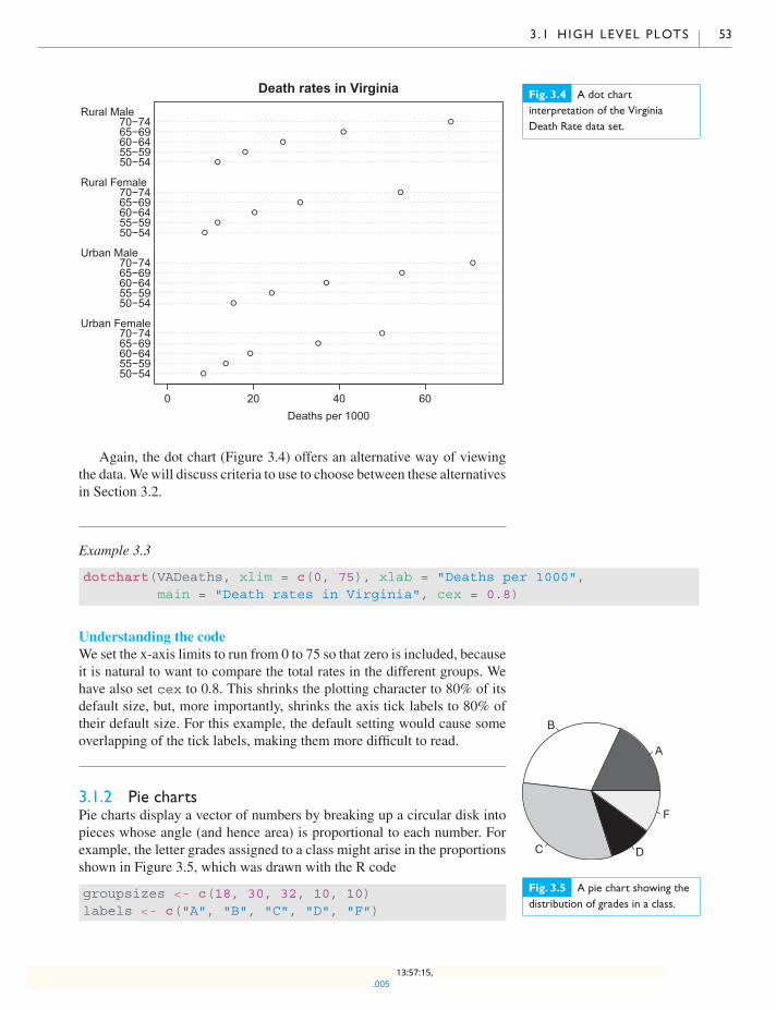
3 .1 HIGH LEVEL PLOTS 53
50−5455−5960−6465−6970−74
50−5455−5960−6465−6970−74
50−5455−5960−6465−6970−74
50−5455−5960−6465−6970−74
●
●
●
●
●
●
●
●
●
●
●
●
●
●
●
●
●
●
●
●Rural Male
Rural Female
Urban Male
Urban Female
0 20 40 60
Death rates in Virginia
Deaths per 1000
Fig. 3.4 A dot chartinterpretation of the VirginiaDeath Rate data set.
Again, the dot chart (Figure 3.4) offers an alternative way of viewingthe data.Wewill discuss criteria to use to choose between these alternativesin Section 3.2.
Example 3.3
dotchart(VADeaths, xlim = c(0, 75), xlab = "Deaths per 1000",main = "Death rates in Virginia", cex = 0.8)
Understanding the codeWe set the x-axis limits to run from 0 to 75 so that zero is included, becauseit is natural to want to compare the total rates in the different groups. Wehave also set cex to 0.8. This shrinks the plotting character to 80% of itsdefault size, but, more importantly, shrinks the axis tick labels to 80% oftheir default size. For this example, the default setting would cause someoverlapping of the tick labels, making them more difficult to read.
A
B
C D
F
Fig. 3.5 A pie chart showing thedistribution of grades in a class.
3.1.2 Pie chartsPie charts display a vector of numbers by breaking up a circular disk intopieces whose angle (and hence area) is proportional to each number. Forexample, the letter grades assigned to a class might arise in the proportionsshown in Figure 3.5, which was drawn with the R code
groupsizes <- c(18, 30, 32, 10, 10)labels <- c("A", "B", "C", "D", "F")
.00513:57:15,

54 PROGRAMMING STATISTICAL GRAPHICS
Areas of the World's Largest Landmasses
Area (on base 10 log scale)
Fre
quen
cy
4.0 4.5 5.0 5.5 6.0 6.5 7.0 7.5
05
1015
20
Fig. 3.6 Histogram of landmassareas on the log scale, with betteraxis labeling and a title.
pie(groupsizes, labels,col = c("grey40", "white", "grey", "black", "grey90"))
Pie charts are popular in non-technical publications, but they have fallenout of favor with statisticians. Some of the reasons why will be discussedin Section 3.2.
3.1.3 HistogramsA histogram is a special type of bar chart that is used to show the frequencydistribution of a collection of numbers. Each bar represents the count of xvalues that fall in the range indicated by the base of the bar. Usually all barsshould be the same width; this is the default in R. In this case the height ofeach bar is proportional to the number of observations in the correspondinginterval. If bars have different widths, then the area of the bar should beproportional to the count; in this way the height represents the density (i.e.the frequency per unit of x).
In R, hist(x, ...) is the main way to plot histograms. Here x is avector consisting of numeric observations, and optional parameters in ...are used to control the details of the display.
An example of a histogram drawn with the default parameter settingswas given in section 2.6.4. The histogram bars decrease in size, roughlyexponentially, in the direction of increasing area (along the horizontal axis).It is often recommended that measurements from such skewed distributionsbe displayed on a logarithmic scale. This is demonstrated in Figure 3.6,together with better axis labeling and a title. Further improvements areillustrated in Section 3.3.3.
hist(log(1000*islands, 10), xlab = "Area (on base 10 log scale)",main = "Areas of the World’s Largest Landmasses")
If you have n values of x, R, by default, divides the range into approx-imately log2(n) + 1 intervals, giving rise to that number of bars.
.00513:57:15,
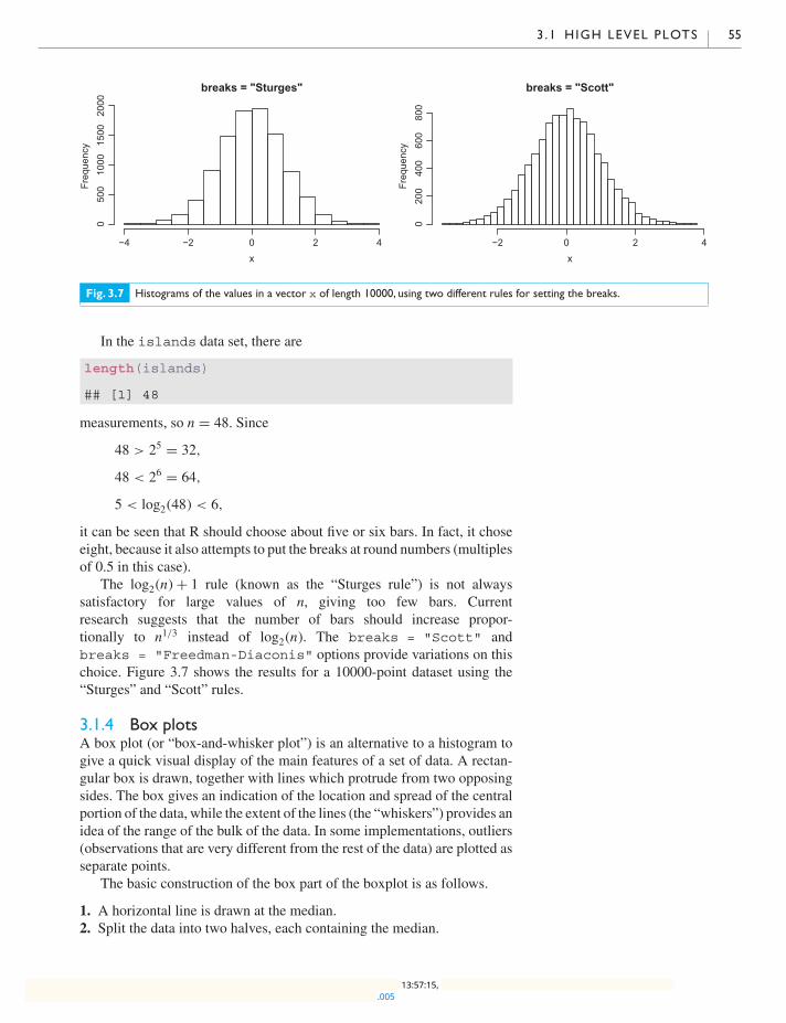
3 .1 HIGH LEVEL PLOTS 55
breaks = "Sturges"
x
Freq
uenc
y
−4 −2 0 2 4
050
010
0015
0020
00breaks = "Scott"
x
Freq
uenc
y
−2 0 2 4
020
040
060
080
0
Fig. 3.7 Histograms of the values in a vector x of length 10000, using two different rules for setting the breaks.
In the islands data set, there are
length(islands)
## [1] 48
measurements, so n = 48. Since
48 > 25 = 32,
48 < 26 = 64,
5 < log2(48) < 6,
it can be seen that R should choose about five or six bars. In fact, it choseeight, because it also attempts to put the breaks at round numbers (multiplesof 0.5 in this case).
The log2(n) + 1 rule (known as the “Sturges rule”) is not alwayssatisfactory for large values of n, giving too few bars. Currentresearch suggests that the number of bars should increase propor-tionally to n1/3 instead of log2(n). The breaks = "Scott" andbreaks = "Freedman-Diaconis" options provide variations on thischoice. Figure 3.7 shows the results for a 10000-point dataset using the“Sturges” and “Scott” rules.
3.1.4 Box plotsA box plot (or “box-and-whisker plot”) is an alternative to a histogram togive a quick visual display of the main features of a set of data. A rectan-gular box is drawn, together with lines which protrude from two opposingsides. The box gives an indication of the location and spread of the centralportion of the data, while the extent of the lines (the “whiskers”) provides anidea of the range of the bulk of the data. In some implementations, outliers(observations that are very different from the rest of the data) are plotted asseparate points.
The basic construction of the box part of the boxplot is as follows.
1. A horizontal line is drawn at the median.2. Split the data into two halves, each containing the median.
.00513:57:15,

56 PROGRAMMING STATISTICAL GRAPHICS
3. Calculate the upper and lower quartiles as the medians of each half, anddraw horizontal lines at each of these values. Then connect the lines toform a rectangular box.
The box thus drawn defines the interquartile range (IQR). This is thedifference between the upper quartile and the lower quartile. We use theIQR to give a measure of the amount of variability in the central portion ofthe dataset, since about 50% of the data will lie within the box.
The lowerwhisker is drawn from the lower end of the box to the smallestvalue that is no smaller than 1.5 IQR below the lower quartile. Similarly,the upper whisker is drawn from the middle of the upper end of the box tothe largest value that is no larger than 1.5 IQR above the upper quartile. Therationale for these definitions is that when data are drawn from the normaldistribution or other distributions with a similar shape, about 99% of theobservations will fall between the whiskers.
●
●
●
outliers
lower whisker
lower quartile
median
upper quartile
upper whisker
outlier
Fig. 3.8 Construction of aboxplot.
An annotated example of a box plot is displayed in Figure 3.8. Boxplots are convenient for comparing distributions of data in two or morecategories, with a number (say 10 or more) of numerical observations percategory. For example, the iris dataset in R is a well-studied dataset ofmeasurements of 50 flowers from each of three species of iris. Figure 3.9,produced by the code
boxplot(Sepal.Length ˜ Species, data = iris,ylab = "Sepal length (cm)", main = "Iris measurements",boxwex = 0.5)
compares the distributions of the sepal length measurements between thedifferent species. Here we have used R’s formula-based interface to thegraphics function: the syntax Sepal.Length ˜ Species is read as“Sepal.Length depending on Species,” where both are columns of thedata frame specified by data = iris. The boxplot() function drawsseparate side-by-side boxplots for each species. From these, we can see
●
setosa versicolor virginica
4.5
5.0
5.5
6.0
6.5
7.0
7.5
8.0
Iris measurements
Sep
al le
ngth
(cm
)
Fig. 3.9 An example ofside-by-side boxplots.
.00513:57:15,

3 .1 HIGH LEVEL PLOTS 57
substantial differences between the mean lengths for the species, and thatthere is one unusually small specimen among the virginica samples.
3.1.5 ScatterplotsWhen doing statistics, most of the interesting problems have to do withthe relationships between different measurements. To study this, one of themost commonly used plots is the scatterplot, in which points (xi, yi), i =1, . . . , n are drawn using dots or other symbols. These are drawn to showrelationships between the xi and yi values. In R, scatterplots (and manyother kinds of plots) are drawn using the plot() function. Its basic usageis plot(x, y, ...) where x and y are numeric vectors of the samelength holding the data to be plotted. There are many additional optionalarguments, and versions of plot designed for non-numerical data as well.
One important optional argument is type. The default istype = "p", which draws a scatterplot. Line plots (in which linesegments join the (xi, yi) points in order from first to last) are drawn usingtype = "l". Many other types are available, including type = "n",to draw nothing: this just sets up the frame around the plot, allowing otherfunctions to be used to draw in it. Some of these other functions will bediscussed in Section 3.3.
Many other types of graphs can be obtained with this function. We willshow how to explore some of the options using some artificial data. Twovectors of numbers will be simulated, one from a standard normal distribu-tion and the other from a Poisson distribution having mean 30.1
1 See Chapter 5 for more informationon the simulation of normal and Poissonrandom variables.
x <- rnorm(100) # assigns 100 random normal observations to xy <- rpois(100, 30) # assigns 100 random Poisson observations
# to y; mean value is 30mean(y) # the resulting value should be near 30
## [1] 30.91
The main argument sets the main title for the plot. Figure 3.10 showsthe result of
plot(x, y, main = "Poisson versus Normal")
Other possibilities you should try:
plot(x, y, pch = 16) # changes the plot symbol to a solid dotplot(x, y, type = ’l’) # plots a broken line (a dense tangle of line
# segments here)plot(sort(x), sort(y), type = ’l’) # a plot of the sample "quantiles"
3.1.6 Plotting data from data frames
Example 3.4The Orange data frame is in the datasets package installed with R. Itconsists of 35 observations on the age (in days since December 31, 1968)
.00513:57:15,
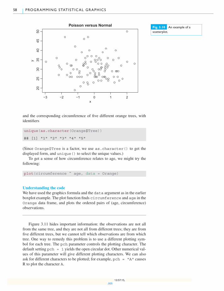
58 PROGRAMMING STATISTICAL GRAPHICS
−3 −2 −1 0 1 2
2025
3035
4045
50
Poisson versus Normal
x
yFig. 3.10 An example of ascatterplot.
and the corresponding circumference of five different orange trees, withidentifiers
unique(as.character(Orange$Tree))
## [1] "1" "2" "3" "4" "5"
(Since Orange$Tree is a factor, we use as.character() to get thedisplayed form, and unique() to select the unique values.)
To get a sense of how circumference relates to age, we might try thefollowing:
plot(circumference ˜ age, data = Orange)
Understanding the codeWe have used the graphics formula and the data argument as in the earlierboxplot example. The plot function finds circumference and age in theOrange data frame, and plots the ordered pairs of (age, circumference)observations.
Figure 3.11 hides important information: the observations are not allfrom the same tree, and they are not all from different trees; they are fromfive different trees, but we cannot tell which observations are from whichtree. One way to remedy this problem is to use a different plotting sym-bol for each tree. The pch parameter controls the plotting character. Thedefault setting pch = 1 yields the open circular dot. Other numerical val-ues of this parameter will give different plotting characters. We can alsoask for different characters to be plotted; for example, pch = "A" causesR to plot the character A.
.00513:57:15,
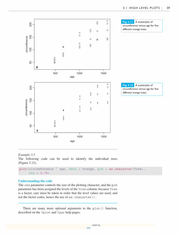
3 .1 HIGH LEVEL PLOTS 59
●
●
●
●●
● ●
●
●
●
●
●
● ●
●
●
●
●●
● ●
●
●
●
●
●
●●
●
●
●
●
●
● ●
500 1000 1500
5010
015
020
0
age
circ
umfe
renc
e
Fig. 3.11 A scatterplot ofcircumference versus age for fivedifferent orange trees.
1
1
1
1 1
1 1
2
2
2
2
2
2 2
3
3
3
33
3 3
4
4
4
44
4 4
5
5
5
5
5
5 5
500 1000 1500
5010
015
020
0
age
circ
umfe
renc
e
Fig. 3.12 A scatterplot ofcircumference versus age for fivedifferent orange trees.
Example 3.5The following code can be used to identify the individual trees(Figure 3.12).
plot(circumference ˜ age, data = Orange, pch = as.character(Tree),cex = 0.75)
Understanding the codeThe cex parameter controls the size of the plotting character, and the pchparameter has been assigned the levels of the Tree column; because Treeis a factor, care must be taken in order that the level values are used, andnot the factor codes, hence the use of as.character().
There are many more optional arguments to the plot() function,described on the ?plot and ?par help pages.
.00513:57:15,

60 PROGRAMMING STATISTICAL GRAPHICS
3.1.7 QQ plotsQuantile–quantile plots (otherwise known as QQ plots) are a type of scat-terplot used to compare the distributions of two groups or to compare asample with a reference distribution.
In the case where there are two groups of equal size, the QQ plot isobtained by first sorting the observations in each group: X[1] ≤ · · · ≤ X[n]and Y [1] ≤ · · · ≤ Y [n]. Next, draw a scatterplot of (X[i],Y [i]), for i =1, . . . , n.
When the groups are of different sizes, some scheme must be usedto artificially match them. R reduces the size of the larger group to thesize of the smaller one by keeping the minimum and maximum values,and choosing equally spaced quantiles between. For example, if there werefive X values but 20 Y values, then the X values would be plotted againstthe minimum, lower quartile, median, upper quartile, and maximum of theY values.
When plotting a single sample against a reference distribution, theoret-ical quantiles are used for one coordinate. R normally puts the theoreticalquantiles on the X axis and the data on the Y axis, but some authors makethe opposite choice. To avoid biases, quantiles are chosen corresponding toprobabilities (i− 1/2)/n: these are centred evenly between zero and one.
When the distributions of X and Y match, the points in the QQ plot willlie near the line y = x. We will see a different straight line if one distribu-tion is a linear transformation of the other. On the other hand, if the twodistributions are not the same, we will see systematic patterns in the QQplot.
Example 3.6The following code illustrates some common patterns (see Figure 3.13),using simulated data.
par(mfrow = c(1,4))X <- rnorm(1000)A <- rnorm(1000)qqplot(X, A, main = "A and X are the same")
B <- rnorm(1000, mean = 3, sd = 2)qqplot(X, B, main = "B is rescaled X")
C <- rt(1000, df = 2)qqplot(X, C, main = "C has heavier tails")
D <- rexp(1000)qqplot(X, D, main = "D is skewed to the right")
Understanding the codeThe mfrow parameter of the par() function is giving a 1 × 4 layout (seeSection 3.3.4). The first plot is based on identical normal distributions, the
.00513:57:15,
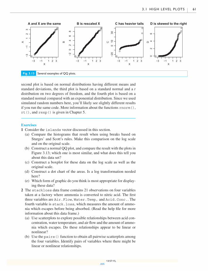
3 .1 HIGH LEVEL PLOTS 61
●●●●●●●●●●●●●●●●●●●●●●●●●●●●●●●●●●●●●●●●●●●●●●●●●●●●●●●●●●●●●●●●●●●●●●●●●●●●●●●●●●●●●●●●●●●●●●●●●●●●●●●●●●●●●●●●●●●●●●●●●●●●●●●●●●●●●●●●●●●●●●●●●●●●●●●●●●●●●●●●●●●●●●●●●●●●●●●●●●●●●●●●●●●●●●●●●●●●●●●●●●●●●●●●●●●●●●●●●●●●●●●●●●●●●●●●●●●●●●●●●●●●●●●●●●●●●●●●●●●●●●●●●●●●●●●●●●●●●●●●●●●●●●●●●●●●●●●●●●●●●●●●●●●●●●●●●●●●●●●●●●●●●●●●●●●●●●●●●●●●●●●●●●●●●●●●●●●●●●●●●●●●●●●●●●●●●●●●●●●●●●●●●●●●●●●●●●●●●●●●●●●●●●●●●●●●●●●●●●●●●●●●●●●●●●●●●●●●●●●●●●●●●●●●●●●●●●●●●●●●●●●●●●●●●●●●●●●●●●●●●●●●●●●●●●●●●●●●●●●●●●●●●●●●●●●●●●●●●●●●●●●●●●●●●●●●●●●●●●●●●●●●●●●●●●●●●●●●●●●●●●●●●●●●●●●●●●●●●●●●●●●●●●●●●●●●●●●●●●●●●●●●●●●●●●●●●●●●●●●●●●●●●●●●●●●●●●●●●●●●●●●●●●●●●●●●●●●●●●●●●●●●●●●●●●●●●●●●●●●●●●●●●●●●●●●●●●●●●●●●●●●●●●●●●●●●●●●●●●●●●●●●●●●●●●●●●●●●●●●●●●●●●●●●●●●●●●●●●●●●●●●●●●●●●●●●●●●●●●●●●●●●●●●●●●●●●●●●●●●●●●●●●●●●●●●●●●●●●●●●●●●●●●●●●●●●●●●●●●●●●●●●●●●●●●●●●●●●●●●●●●●●●●●●●●●●●●●●●●●●●●●●●●●●●●●●●●●●●●●●●●●●●●●●●●●●●●●●●●●●●●●●●●●●●●●●●●●●●●●●●●●●●●●●●●●●●●●●●●●●●●●●●●●●●●●●●●●●●●●●●●●●●●●●●●●●●●●●●●
●●
−3 −1 1 2 3
−3−1
12
3A and X are the same
X
A
● ●●●●●●●●●●●●●●●●●●●●●●●●●●●●●●●●●●●●●●●●●●●●●●●●●●●●●●●●●●●●●●●●●●●●●●●●●●●●●●●●●●●●●●●●●●●●●●●●●●●●●●●●●●●●●●●●●●●●●●●●●●●●●●●●●●●●●●●●●●●●●●●●●●●●●●●●●●●●●●●●●●●●●●●●●●●●●●●●●●●●●●●●●●●●●●●●●●●●●●●●●●●●●●●●●●●●●●●●●●●●●●●●●●●●●●●●●●●●●●●●●●●●●●●●●●●●●●●●●●●●●●●●●●●●●●●●●●●●●●●●●●●●●●●●●●●●●●●●●●●●●●●●●●●●●●●●●●●●●●●●●●●●●●●●●●●●●●●●●●●●●●●●●●●●●●●●●●●●●●●●●●●●●●●●●●●●●●●●●●●●●●●●●●●●●●●●●●●●●●●●●●●●●●●●●●●●●●●●●●●●●●●●●●●●●●●●●●●●●●●●●●●●●●●●●●●●●●●●●●●●●●●●●●●●●●●●●●●●●●●●●●●●●●●●●●●●●●●●●●●●●●●●●●●●●●●●●●●●●●●●●●●●●●●●●●●●●●●●●●●●●●●●●●●●●●●●●●●●●●●●●●●●●●●●●●●●●●●●●●●●●●●●●●●●●●●●●●●●●●●●●●●●●●●●●●●●●●●●●●●●●●●●●●●●●●●●●●●●●●●●●●●●●●●●●●●●●●●●●●●●●●●●●●●●●●●●●●●●●●●●●●●●●●●●●●●●●●●●●●●●●●●●●●●●●●●●●●●●●●●●●●●●●●●●●●●●●●●●●●●●●●●●●●●●●●●●●●●●●●●●●●●●●●●●●●●●●●●●●●●●●●●●●●●●●●●●●●●●●●●●●●●●●●●●●●●●●●●●●●●●●●●●●●●●●●●●●●●●●●●●●●●●●●●●●●●●●●●●●●●●●●●●●●●●●●●●●●●●●●●●●●●●●●●●●●●●●●●●●●●●●●●●●●●●●●●●●●●●●●●●●●●●●●●●●●●●●●●●●●●●●●●●●●●●●●●●●●●●●●●●●●●●●●●●●●●●●●●●●●●●●●●●●
●●●●●●●●●●●
●●●
−3 −1 1 2 3
−20
24
68
B is rescaled X
XB
●
●●●●●●●●●●●●●●●●●●●●●●●●●●●●●●●●●●●●●●●●●●●●●●●●●●●●●●●●●●●●●●●●●●●●●●●●●●●●●●●●●●
●●●●●●●●●●●●●●●●●●●●●●●●●●●●●●●●●●●●●●●●●●●●●●●●●●●●●●●●●●●●●●●●●●●●●●●●●●●●●●●●●●●●●●●●●●●●●●●●●●●●●●●●●●●●●●●●●●●●●●●●●●●●●●●●●●●●●●●●●●●●●●●●●●●●●●●●●●●●●●●●●●●●●●●●●●●●●●●●●●●●●●●●●●●●●●●●●●●●●●●●●●●●●●●●●●●●●●●●●●●●●●●●●●●●●●●●●●●●●●●●●●●●●●●●●●●●●●●●●●●●●●●●●●●●●●●●●●●●●●●●●●●●●●●●●●●●●●●●●●●●●●●●●●●●●●●●●●●●●●●●●●●●●●●●●●●●●●●●●●●●●●●●●●●●●●●●●●●●●●●●●●●●●●●●●●●●●●●●●●●●●●●●●●●●●●●●●●●●●●●●●●●●●●●●●●●●●●●●●●●●●●●●●●●●●●●●●●●●●●●●●●●●●●●●●●●●●●●●●●●●●●●●●●●●●●●●●●●●●●●●●●●●●●●●●●●●●●●●●●●●●●●●●●●●●●●●●●●●●●●●●●●●●●●●●●●●●●●●●●●●●●●●●●●●●●●●●●●●●●●●●●●●●●●●●●●●●●●●●●●●●●●●●●●●●●●●●●●●●●●●●●●●●●●●●●●●●●●●●●●●●●●●●●●●●●●●●●●●●●●●●●●●●●●●●●●●●●●●●●●●●●●●●●●●●●●●●●●●●●●●●●●●●●●●●●●●●●●●●●●●●●●●●●●●●●●●●●●●●●●●●●●●●●●●●●●●●●●●●●●●●●●●●●●●●●●●●●●●●●●●●●●●●●●●●●●●●●●●●●●●●●●●●●●●●●●●●●●●●●●●●●●●●●●●●●●●●●●●●
●●●●●●●●●●●●●●●●●●●●●●●●●●●●●●●●●●●●●●●●●●●●●●●●●●●●●●●●●●●●●●●●●●●●●●●●●●●●●●●●●●●●●
●●●●●●●●●●●●●
●
●
−3 −1 1 2 3
−20
010
30
C has heavier tails
X
C
● ●●●●●●●●●●●●●●●●●●●●●●●●●●●●●●●●●●●●●●●●●●●●●●●●●●●●●●●●●●●●●●●●●●●●●●●●●●●●●●●●●●●●●●●●●●●●●●●●●●●●●●●●●●●●●●●●●●●●●●●●●●●●●●●●●●●●●●●●●●●●●●●●●●●●●●●●●●●●●●●●●●●●●●●●●●●●●●●●●●●●●●●●●●●●●●●●●●●●●●●●●●●●●●●●●●●●●●●●●●●●●●●●●●●●●●●●●●●●●●●●●●●●●●●●●●●●●●●●●●●●●●●●●●●●●●●●●●●●●●●●●●●●●●●●●●●●●●●●●●●●●●●●●●●●●●●●●●●●●●●●●●●●●●●●●●●●●●●●●●●●●●●●●●●●●●●●●●
●●●●●●●●●●●●●●●●●●●●●●●●●●●●●●●●●●●●●●●●●●●●●●●●●●●●●●●●●●●●●●●●●●●●●●●●●●●●●●●●●●●●●●●●●●●●●●●●●●●●●●●●●●●●●●●●●●●●●●●●●●●●●●●●●●●●●●●●●●●●●●●●●●●●●●●●●●●●●●●●●●●●●●●●●●●●●●●●●●●●●●●●●●●●●●●●●●●●●●●●●●●●●●●●●●●●●●●●●●●●●●●●●●●●●●●●●●●●●●●●●●●●●●●●●●●●●●●●●●●●●●●●●●●●●●●●●●●●●●●●●●●●●●●●●●●●●●●●●●●●●●●●●●●●●●●●●●●●●●●●●●●●●●●●●●●●●●●●●●●●●●●●●●●●●●●●●●●●●●●●●●●●●●●●●●●●●●●●●●●●●●●●●●●●●●●●●●●●●●●●●●●●●●●●●●●●●●●●●●●●●●●●●●●●●●●●●●●●●●●●●●●●●●●●●●●●●●●●●●●●●●●●●●●●●●●●●●●●●●●●●●●●●●●●●●●●●●●●●●●●●●●●●●●●●●●●●●●●●●●●●●●●●●●●●●●●●●●●●●●●●●●●●●●●●●●●●●●●●●●●●●●●●●●●●●●●●●●●●●●●●●●●●●●●●●●●●●●●●●●●●●●●●●●●●●●●●●●●●●●●●●●●●●●●●●●●●●●●●●●●●●●
●
●
−3 −1 1 2 3
02
46
D is skewed to the right
X
D
Fig. 3.13 Several examples of QQ plots.
second plot is based on normal distributions having different means andstandard deviations, the third plot is based on a standard normal and a tdistribution on two degrees of freedom, and the fourth plot is based on astandard normal compared with an exponential distribution. Since we usedsimulated random numbers here, you’ll likely see slightly different resultsif you run the same code. More information about the functions rnorm(),rt(), and rexp() is given in Chapter 5.
Exercises1 Consider the islands vector discussed in this section.
(a) Compare the histograms that result when using breaks based onSturges’ and Scott’s rules. Make this comparison on the log scaleand on the original scale.
(b) Construct a normal QQ plot, and compare the result with the plots inFigure 3.13; which one is most similar, and what does this tell youabout this data set?
(c) Construct a boxplot for these data on the log scale as well as theoriginal scale.
(d) Construct a dot chart of the areas. Is a log transformation neededhere?
(e) Which form of graphic do you think is most appropriate for display-ing these data?
2 The stackloss data frame contains 21 observations on four variablestaken at a factory where ammonia is converted to nitric acid. The firstthree variables are Air.Flow, Water.Temp, and Acid.Conc.. Thefourth variable is stack.loss, which measures the amount of ammo-nia which escapes before being absorbed. (Read the help file for moreinformation about this data frame.)(a) Use scatterplots to explore possible relationships between acid con-
centration, water temperature, and air flow and the amount of ammo-nia which escapes. Do these relationships appear to be linear ornonlinear?
(b) Use the pairs() function to obtain all pairwise scatterplots amongthe four variables. Identify pairs of variables where there might belinear or nonlinear relationships.
.00513:57:15,
62 PROGRAMMING STATISTICAL GRAPHICS
3 Consider the pressure data frame. There are two columns –temperature and pressure.(a) Construct a scatterplot with pressure on the vertical axis and
temperature on the horizontal axis. Are the variables related lin-early or nonlinearly?
(b) The graph of the following function passes through the plotted pointsreasonably well:
y = (0.168 + 0.007x)20/3.
The differences between the pressure values predicted by the curveand the observed pressure values are called residuals. Here is a wayto calculate them:
residuals <- with(pressure, pressure -(0.168 + 0.007*temperature)ˆ(20/3))
Construct a normal QQ plot of these residuals and decide whetherthey are normally distributed or whether they follow a skeweddistribution.
(c) Now, apply the power transformation y3/20 to the pressure data val-ues. Plot these transformed values against temperature. Is a linear ornonlinear relationship evident now?
(d) Calculate residuals for the difference between transformed pressurevalues and those predicted by the straight line. Obtain a normal QQplot, and decide whether the residuals follow a normal distributionor not.
3.2 Choosing a high level graphic
We have described bar, dot, and pie charts, histograms, boxplots, scatter-plots, and QQ plots. There are many other styles of statistical graphics thatwe haven’t discussed. How should a user choose which one to use?
The first consideration is the type of data. As discussed in the previoussection, bar, dot, and pie charts display individual values, histograms, box-plots and QQ plots display distributions, and scatterplots display pairs ofvalues.
Another consideration is the audience. If the plot is for yourself or fora statistically educated audience, then you can assume a more sophisti-cated understanding. For example, a boxplot or QQplot would requiremoreexplanation than a histogram, and might not be appropriate for the generalpublic.
It is also important to have some understanding of how human visualperception works in order to make a good choice. There has been a hugeamount of research on this and we can only touch on it here.
When looking at a graph, you extract quantitative information whenyour visual system decodes the graph. This process can be described interms of unconscious measurements of lengths, positions, slopes, angles,areas, volumes, and various aspects of color. It has been found that peopleare particularly good at recognizing lengths and positions, not as good atslopes and angles, and their perception of areas and volumes can be quite
.00513:57:15,
3 .3 LOW LEVEL GRAPHICS FUNCTIONS 63
inaccurate, depending on the shape. Most of us are quite good at recogniz-ing differences in colors. However, up to 10% of men and a much smallerproportion of women are partially color-blind, and hardly anyone is verygood at making quantitative measurements from colors.
We can take these facts about perception into account when we con-struct graphs. We should try to convey the important information in waysthat are easy to perceive, and we should try not to have conflicting messagesin a graph.
For example, the bars in bar charts are easy to recognize, because thepositions of the ends of the bars and the lengths of the bars are easy to see.The area of the bars also reinforces our perception.
However, the fact that we see length and area when we look at a barconstrains us. We should normally base bar charts at zero, so that the posi-tion, length, and area all convey the same information. If we are displayingnumbers where zero is not relevant, then a dot chart is a better choice: in adot chart it is mainly the position of the dot that is perceived.
Thinking in terms of visual tasks tells us that pie charts can be poorchoices for displaying data. In order to see the sizes of slices of the pie, weneed to make angle and area measurements, and we are not very good atthose.
Finally, color can be very useful in graphs to distinguish groups fromeach other. The RColorBrewer package in R contains a number ofpalettes, or selections of colors. Some palettes indicate sequential groupsfrom low to high, others show groups that diverge from a neutral value, andothers are purely qualitative. These are chosen so that most people (even ifcolor-blind) can easily see the differences.
3.3 Low level graphics functions
Functions like barplot(), dotchart(), and plot() do their workby using low level graphics functions to draw lines and points, to establishwhere they will be placed on a page, and so on.
In this section wewill describe some of these low level functions, whichare also available to users to customize their plots. We will start with adescription of how R views the page it is drawing on, then show how to addpoints, lines, and text to existing plots, and finish by showing how some ofthe common graphics settings are changed.
3.3.1 The plotting region and marginsBase graphics in R divides up the display into several regions. The plotregion is where data will be drawn. Within the plot region R maintains acoordinate system based on the data. The axes show this coordinate system.Outside the plot region are the margins, numbered clockwise from 1 to 4,starting at the bottom. Normally text and labels are plotted in the margins,and R positions objects based on a count of lines out from the plot region.Figure 3.14 illustrates this. (We give the code that produced this plot inExample 3.8.) We can see from the figure that R chose to draw the tickmark labels on line 1. We drew the margin titles on line 3.
.00513:57:15,
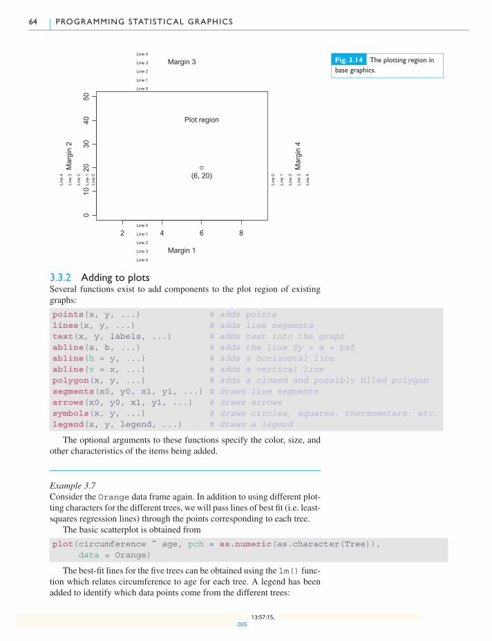
64 PROGRAMMING STATISTICAL GRAPHICS
2 4 6 8
010
2030
4050
Plot region
●
(6, 20)
Margin 1
Mar
gin
2Margin 3
Mar
gin
4
Line 0
Line 1
Line 2
Line 3
Line 4
Line
0Li
ne 1
Line
2
Line
3
Line
4
Line 0
Line 1
Line 2
Line 3
Line 4
Line
0
Line
1
Line
2
Line
3
Line
4
Fig. 3.14 The plotting region inbase graphics.
3.3.2 Adding to plotsSeveral functions exist to add components to the plot region of existinggraphs:
points(x, y, ...) # adds pointslines(x, y, ...) # adds line segmentstext(x, y, labels, ...) # adds text into the graphabline(a, b, ...) # adds the line $y = a + bx$abline(h = y, ...) # adds a horizontal lineabline(v = x, ...) # adds a vertical linepolygon(x, y, ...) # adds a closed and possibly filled polygonsegments(x0, y0, x1, y1, ...) # draws line segmentsarrows(x0, y0, x1, y1, ...) # draws arrowssymbols(x, y, ...) # draws circles, squares, thermometers, etc.legend(x, y, legend, ...) # draws a legend
The optional arguments to these functions specify the color, size, andother characteristics of the items being added.
Example 3.7Consider the Orange data frame again. In addition to using different plot-ting characters for the different trees, we will pass lines of best fit (i.e. least-squares regression lines) through the points corresponding to each tree.
The basic scatterplot is obtained from
plot(circumference ˜ age, pch = as.numeric(as.character(Tree)),data = Orange)
The best-fit lines for the five trees can be obtained using the lm() func-tion which relates circumference to age for each tree. A legend has beenadded to identify which data points come from the different trees:
.00513:57:15,
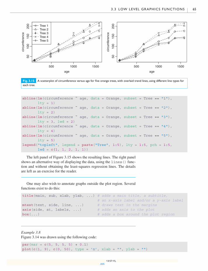
3 .3 LOW LEVEL GRAPHICS FUNCTIONS 65
●
●
●
●●
● ●
500 1000 1500
5010
015
020
0
age
circ
umfe
renc
e● Tree 1
Tree 2Tree 3Tree 4Tree 5
●
●
●
●●
● ●
500 1000 1500
5010
015
020
0
age
circ
umfe
renc
e
Fig. 3.15 A scatterplot of circumference versus age for five orange trees, with overlaid trend lines, using different line types foreach tree.
abline(lm(circumference ˜ age, data = Orange, subset = Tree == "1"),lty = 1)
abline(lm(circumference ˜ age, data = Orange, subset = Tree == "2"),lty = 2)
abline(lm(circumference ˜ age, data = Orange, subset = Tree == "3"),lty = 3, lwd = 2)
abline(lm(circumference ˜ age, data = Orange, subset = Tree == "4"),lty = 4)
abline(lm(circumference ˜ age, data = Orange, subset = Tree == "5"),lty = 5)
legend("topleft", legend = paste("Tree", 1:5), lty = 1:5, pch = 1:5,lwd = c(1, 1, 2, 1, 1))
The left panel of Figure 3.15 shows the resulting lines. The right panelshows an alternative way of displaying the data, using the lines() func-tion and without obtaining the least-squares regression lines. The detailsare left as an exercise for the reader.
One may also wish to annotate graphs outside the plot region. Severalfunctions exist to do this:
title(main, sub, xlab, ylab, ...) # adds a main title, a subtitle,# an x-axis label and/or a y-axis label
mtext(text, side, line, ...) # draws text in the marginsaxis(side, at, labels, ...) # adds an axis to the plotbox(...) # adds a box around the plot region
Example 3.8Figure 3.14 was drawn using the following code:
par(mar = c(5, 5, 5, 5) + 0.1)plot(c(1, 9), c(0, 50), type = ’n’, xlab = "", ylab = "")
.00513:57:15,
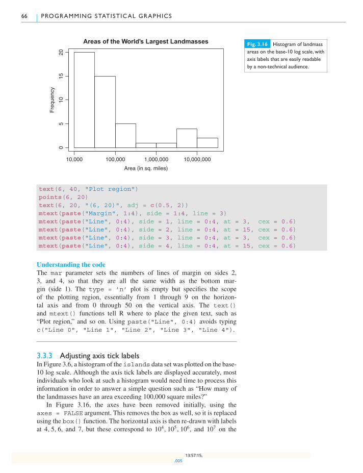
66 PROGRAMMING STATISTICAL GRAPHICS
Areas of the World's Largest Landmasses
Area (in sq. miles)
Fre
quen
cy
10,000 100,000 1,000,000 10,000,000
05
1015
20
Fig. 3.16 Histogram of landmassareas on the base-10 log scale, withaxis labels that are easily readableby a non-technical audience.
text(6, 40, "Plot region")points(6, 20)text(6, 20, "(6, 20)", adj = c(0.5, 2))mtext(paste("Margin", 1:4), side = 1:4, line = 3)mtext(paste("Line", 0:4), side = 1, line = 0:4, at = 3, cex = 0.6)mtext(paste("Line", 0:4), side = 2, line = 0:4, at = 15, cex = 0.6)mtext(paste("Line", 0:4), side = 3, line = 0:4, at = 3, cex = 0.6)mtext(paste("Line", 0:4), side = 4, line = 0:4, at = 15, cex = 0.6)
Understanding the codeThe mar parameter sets the numbers of lines of margin on sides 2,3, and 4, so that they are all the same width as the bottom mar-gin (side 1). The type = ’n’ plot is empty but specifies the scopeof the plotting region, essentially from 1 through 9 on the horizon-tal axis and from 0 through 50 on the vertical axis. The text()and mtext() functions tell R where to place the given text, such as“Plot region,” and so on. Using paste("Line", 0:4) avoids typingc("Line 0", "Line 1", "Line 2", "Line 3", "Line 4").
3.3.3 Adjusting axis tick labelsIn Figure 3.6, a histogram of the islands data set was plotted on the base-10 log scale. Although the axis tick labels are displayed accurately, mostindividuals who look at such a histogram would need time to process thisinformation in order to answer a simple question such as “How many ofthe landmasses have an area exceeding 100,000 square miles?”
In Figure 3.16, the axes have been removed initially, using theaxes = FALSE argument. This removes the box as well, so it is replacedusing the box() function. The horizontal axis is then re-drawn with labelsat 4, 5, 6, and 7, but these correspond to 104, 105, 106, and 107 on the
.00513:57:15,
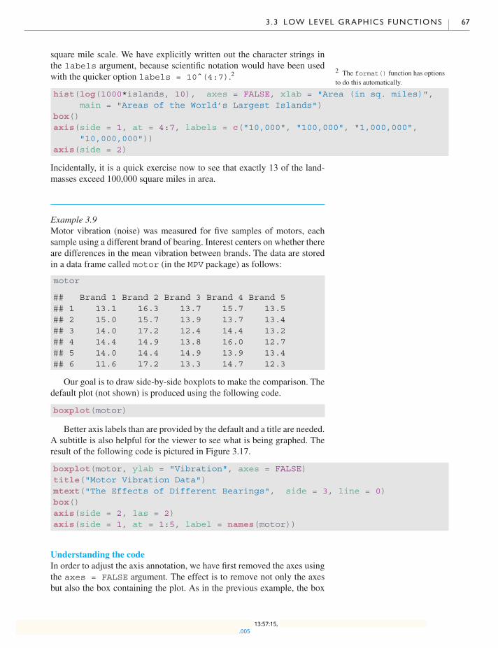
3 .3 LOW LEVEL GRAPHICS FUNCTIONS 67
square mile scale. We have explicitly written out the character strings inthe labels argument, because scientific notation would have been usedwith the quicker option labels = 10ˆ(4:7).2
2 The format() function has optionsto do this automatically.
hist(log(1000*islands, 10), axes = FALSE, xlab = "Area (in sq. miles)",main = "Areas of the World’s Largest Islands")
box()axis(side = 1, at = 4:7, labels = c("10,000", "100,000", "1,000,000",
"10,000,000"))axis(side = 2)
Incidentally, it is a quick exercise now to see that exactly 13 of the land-masses exceed 100,000 square miles in area.
Example 3.9Motor vibration (noise) was measured for five samples of motors, eachsample using a different brand of bearing. Interest centers on whether thereare differences in the mean vibration between brands. The data are storedin a data frame called motor (in the MPV package) as follows:
motor
## Brand 1 Brand 2 Brand 3 Brand 4 Brand 5## 1 13.1 16.3 13.7 15.7 13.5## 2 15.0 15.7 13.9 13.7 13.4## 3 14.0 17.2 12.4 14.4 13.2## 4 14.4 14.9 13.8 16.0 12.7## 5 14.0 14.4 14.9 13.9 13.4## 6 11.6 17.2 13.3 14.7 12.3
Our goal is to draw side-by-side boxplots to make the comparison. Thedefault plot (not shown) is produced using the following code.
boxplot(motor)
Better axis labels than are provided by the default and a title are needed.A subtitle is also helpful for the viewer to see what is being graphed. Theresult of the following code is pictured in Figure 3.17.
boxplot(motor, ylab = "Vibration", axes = FALSE)title("Motor Vibration Data")mtext("The Effects of Different Bearings", side = 3, line = 0)box()axis(side = 2, las = 2)axis(side = 1, at = 1:5, label = names(motor))
Understanding the codeIn order to adjust the axis annotation, we have first removed the axes usingthe axes = FALSE argument. The effect is to remove not only the axesbut also the box containing the plot. As in the previous example, the box
.00513:57:15,
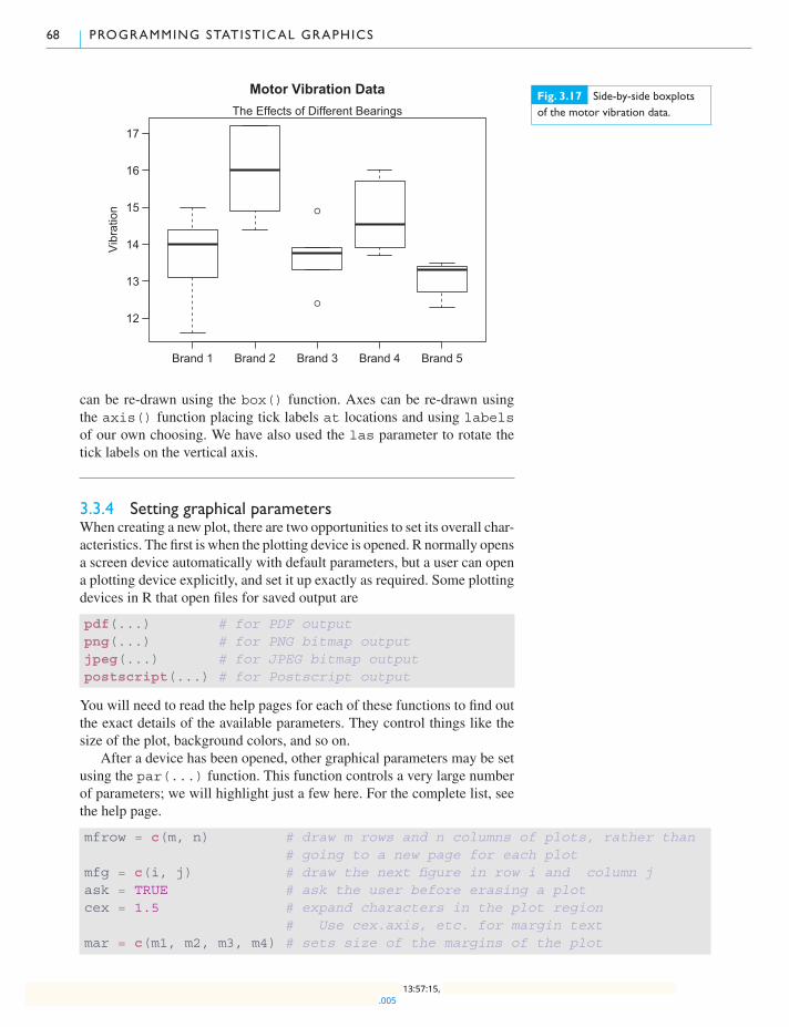
68 PROGRAMMING STATISTICAL GRAPHICS
●
●
Vib
ratio
n
Motor Vibration DataThe Effects of Different Bearings
12
13
14
15
16
17
Brand 1 Brand 2 Brand 3 Brand 4 Brand 5
Fig. 3.17 Side-by-side boxplotsof the motor vibration data.
can be re-drawn using the box() function. Axes can be re-drawn usingthe axis() function placing tick labels at locations and using labelsof our own choosing. We have also used the las parameter to rotate thetick labels on the vertical axis.
3.3.4 Setting graphical parametersWhen creating a new plot, there are two opportunities to set its overall char-acteristics. The first is when the plotting device is opened. R normally opensa screen device automatically with default parameters, but a user can opena plotting device explicitly, and set it up exactly as required. Some plottingdevices in R that open files for saved output are
pdf(...) # for PDF outputpng(...) # for PNG bitmap outputjpeg(...) # for JPEG bitmap outputpostscript(...) # for Postscript output
You will need to read the help pages for each of these functions to find outthe exact details of the available parameters. They control things like thesize of the plot, background colors, and so on.
After a device has been opened, other graphical parameters may be setusing the par(...) function. This function controls a very large numberof parameters; we will highlight just a few here. For the complete list, seethe help page.
mfrow = c(m, n) # draw m rows and n columns of plots, rather than# going to a new page for each plot
mfg = c(i, j) # draw the next figure in row i and column jask = TRUE # ask the user before erasing a plotcex = 1.5 # expand characters in the plot region
# Use cex.axis, etc. for margin textmar = c(m1, m2, m3, m4) # sets size of the margins of the plot
.00513:57:15,
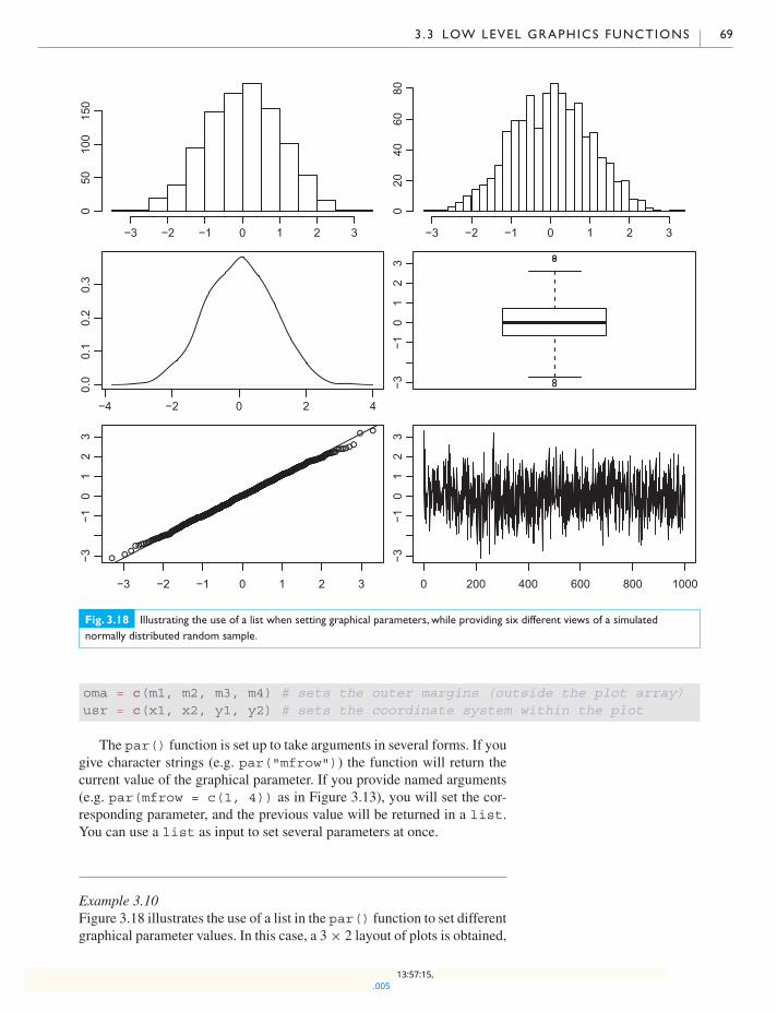
3 .3 LOW LEVEL GRAPHICS FUNCTIONS 69
−3 −2 −1 0 1 2 3
050
100
150
−3 −2 −1 0 1 2 3
020
4060
80−4 −2 0 2 4
0.0
0.1
0.2
0.3
●
●●
●
−3−1
01
23
●
●
●
●
●●
●
●●
●
●●
●
●●
●
●
●
●●
●
●
●
●●
●
●●
●
●●
●
●
●●
●●●
●
●
●●
●
●
●●
●
●
●●
●
●
●
●
●
●
●
●
●●
●
●●
●●●●
●●●●
●●
●
●●
●
●
●●
●
●
●
●
●●
●●
●
●
●
●
●
●
●
●●
●●
●
●
●
●
●
●
●●
●
●
●
●
●
●
●●
●
●
●
●
●
●●●
●
●
●
●
●
●●●●●
●
●
●●
●●●●●
●●
●●
●
●
●
●●
●
●●
●
●
●●●
●
●
●
●
●
●
●
●
●●
●●
●
●
●
●
●●
●
●●
●
●●●
●
●
●
●●
●
●
●
●
●
●●
●
●
●
●
●
●
●
●
●
●●
●
●
●
●
●
●●
●
●
●●
●
●
●
●
●
●
●
●
●
●
●
●
●
●
●
●
●●●●
●
●●
●
●
●
●
●●
●●
●
●
●
●
●●●●
●
●
●
●
●
●
●
●
●
●
●●
●●●
●
●
●●
●●
●
●
●
●
●
●
●
●
●
●
●
●
●
●●
●
●●
●
●
●●●●
●
●●
●
●
●
●
●●●●
●
●
●
●●
●
●
●
●
●
●
●●
●
●
●
●
●
●
●●
●
●
●
●
●
●
●
●
●
●
●
●
●
●●●
●
●●
●
●●●
●
●
●
●
●
●
●
●
●
●
●
●
●
●
●
●
●
●
●
●●
●●
●●
●●●
●
●
●
●
●
●
●
●
●
●
●
●
●
●
●
●
●
●
●
●
●
●
●●
●
●●
●●
●
●
●
●
●
●●
●
●
●
●
●
●●●●
●
●●
●
●
●●●
●●
●
●
●●
●
●
●●
●
●
●
●
●
●
●
●
●●
●●
●●
●●●
●
●
●
●
●
●
●
●●
●●
●
●
●
●
●
●●●
●
●
●
●
●
●●
●
●
●●●
●
●
●●
●
●●
●
●●
●
●
●●
●●
●
●
●●
●
●●
●
●●
●
●●●
●
●●
●
●
●
●
●
●
●●●
●
●
●
●
●
●
●
●
●
●
●
●
●●
●
●●
●
●
●
●●
●
●
●
●
●
●
●
●●
●
●
●●
●
●
●
●●
●
●
●●
●
●
●
●
●
●
●
●
●
●●●
●●
●●
●
●●●
●
●
●
●●
●
●
●
●
●
●
●●
●
●
●
●
●
●
●●
●●
●
●●●
●
●
●
●
●
●
●
●
●
●●
●
●
●●
●
●
●
●
●
●
●
●
●
●
●●
●
●
●●
●●
●
●
●
●
●
●●
●
●●
●
●
●
●
●
●
●
●
●
●
●
●
●
●
●
●
●
●
●
●
●
●
●
●
●●
●
●
●
●
●●
●
●
●
●
●
●
●●●
●
●
●
●●
●
●●●●
●
●●
●
●
●
●
●
●
●●
●
●
●
●
●●
●
●
●●●
●
●
●
●
●
●
●
●
●●
●●
●
●●
●
●
●
●
●
●●
●
●
●
●
●
●
●
●●
●
●●
●
●
●
●
●
●
●
●
●
●
●
●
●
●
●●●
●
●
●●
●●●●
●
●
●
●
●●
●
●
●
●
●
●
●
●
●
●●●
●
●
●
●
●
●●
●
●
●●
●
●
●
●
●
●
●
●
●
●
●
●
●
●
●
●●
●●
●
●
●
●
●●●●
●
●
●●
●
●
●
●
●●
●
●
●
●
●
●
●
●
●
●●
●
●●
●
●
●
●
●
●
●
●●●
●
●
●
●
●●
●●
●
●
●
●
●●
●
●
●●
●
●
●●
●●●
●
●●●
●
●●
●
●
●
●
●
●
●●
●
●●
●
●
●
●●
●
●
●
●
●
●
●
●
●
●
●●
●●
●
●●●
●
●
●
●
●
●●
●
●
●
●
●
●
●●
●
●
●●●
●
●
●
●
●●
●
●
●
●●
●
●
●●
●
●
●
●
●
−3 −2 −1 0 1 2 3
−3−1
01
23
0 200 400 600 800 1000
−3−1
01
23
Fig. 3.18 Illustrating the use of a list when setting graphical parameters, while providing six different views of a simulatednormally distributed random sample.
oma = c(m1, m2, m3, m4) # sets the outer margins (outside the plot array)usr = c(x1, x2, y1, y2) # sets the coordinate system within the plot
The par() function is set up to take arguments in several forms. If yougive character strings (e.g. par("mfrow")) the function will return thecurrent value of the graphical parameter. If you provide named arguments(e.g. par(mfrow = c(1, 4)) as in Figure 3.13), you will set the cor-responding parameter, and the previous value will be returned in a list.You can use a list as input to set several parameters at once.
Example 3.10Figure 3.18 illustrates the use of a list in the par() function to set differentgraphical parameter values. In this case, a 3 × 2 layout of plots is obtained,
.00513:57:15,
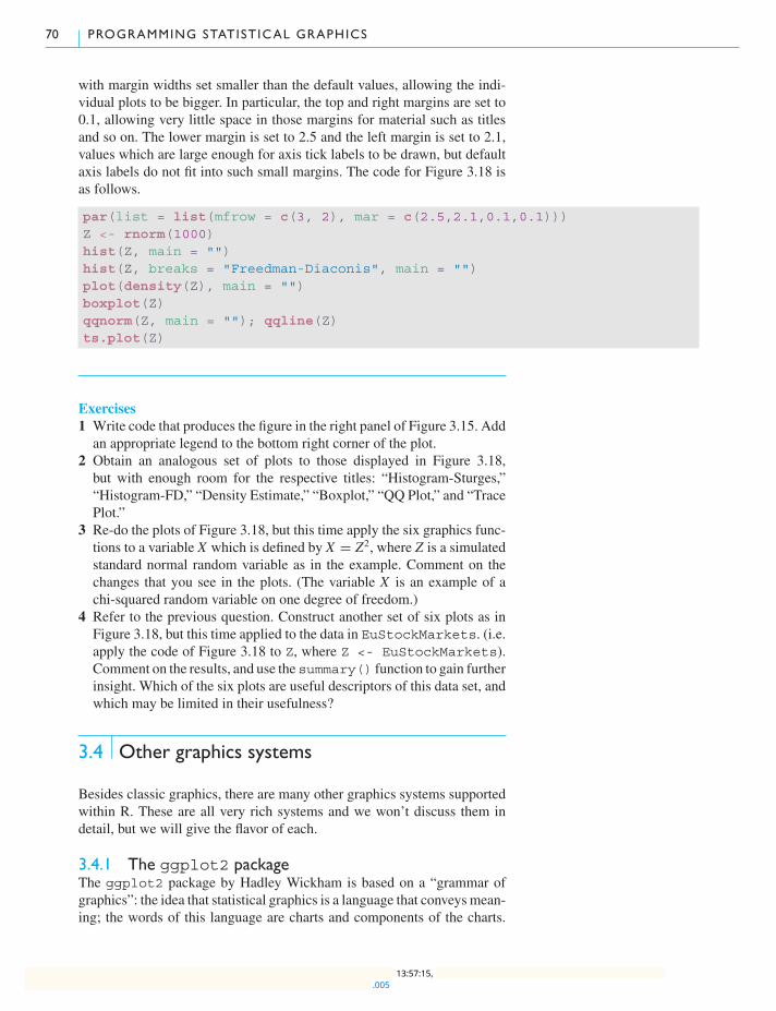
70 PROGRAMMING STATISTICAL GRAPHICS
with margin widths set smaller than the default values, allowing the indi-vidual plots to be bigger. In particular, the top and right margins are set to0.1, allowing very little space in those margins for material such as titlesand so on. The lower margin is set to 2.5 and the left margin is set to 2.1,values which are large enough for axis tick labels to be drawn, but defaultaxis labels do not fit into such small margins. The code for Figure 3.18 isas follows.
par(list = list(mfrow = c(3, 2), mar = c(2.5,2.1,0.1,0.1)))Z <- rnorm(1000)hist(Z, main = "")hist(Z, breaks = "Freedman-Diaconis", main = "")plot(density(Z), main = "")boxplot(Z)qqnorm(Z, main = ""); qqline(Z)ts.plot(Z)
Exercises1 Write code that produces the figure in the right panel of Figure 3.15. Addan appropriate legend to the bottom right corner of the plot.
2 Obtain an analogous set of plots to those displayed in Figure 3.18,but with enough room for the respective titles: “Histogram-Sturges,”“Histogram-FD,” “Density Estimate,” “Boxplot,” “QQ Plot,” and “TracePlot.”
3 Re-do the plots of Figure 3.18, but this time apply the six graphics func-tions to a variable X which is defined by X = Z2, where Z is a simulatedstandard normal random variable as in the example. Comment on thechanges that you see in the plots. (The variable X is an example of achi-squared random variable on one degree of freedom.)
4 Refer to the previous question. Construct another set of six plots as inFigure 3.18, but this time applied to the data in EuStockMarkets. (i.e.apply the code of Figure 3.18 to Z, where Z <- EuStockMarkets).Comment on the results, and use the summary() function to gain furtherinsight. Which of the six plots are useful descriptors of this data set, andwhich may be limited in their usefulness?
3.4 Other graphics systems
Besides classic graphics, there are many other graphics systems supportedwithin R. These are all very rich systems and we won’t discuss them indetail, but we will give the flavor of each.
3.4.1 The ggplot2 packageThe ggplot2 package by Hadley Wickham is based on a “grammar ofgraphics”: the idea that statistical graphics is a language that conveys mean-ing; the words of this language are charts and components of the charts.
.00513:57:15,

3 .4 OTHER GRAPHICS SYSTEMS 71
0
10000
20000
30000
40000
N.Amer Europe Asia S.Amer Oceania Africa Mid.Amer
Region
Tele
phon
esFig. 3.19 Re-doing Figure 3.1using ggplot2.
Rather than describing the ink that goes on the page, the code describes themessage you want to send.
Example 3.11To plot the world phone data that we saw at the start of this chapter, wewould write
library(ggplot2)region <- names(WorldPhones51)phones51 <- data.frame(Region = factor(region, levels = region),
Telephones = WorldPhones51)ggplot(phones51, aes(Region, Telephones)) + geom_bar(stat = "identity")
This says that we want the names on the x-axis, the values on the y-axis.We want to display this using bars. The statistic to display is the identity,i.e. just the value itself. The result is shown in Figure 3.19.
The ggplot2 package gives a very rich way to describe graphics;unfortunately, we don’t have the space to describe it here. Interested read-ers should read The Grammar of Graphics byWilkinson for the underlyingtheory, and ggplot2: Elegant Graphics for Data Analysis by Wickham forthe ggplot2 implementation.
.00513:57:15,
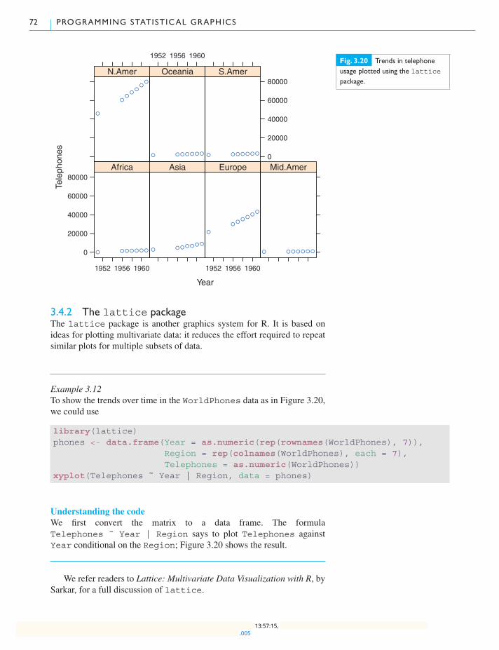
72 PROGRAMMING STATISTICAL GRAPHICS
Year
Tele
phon
es
0
20000
40000
60000
80000
1952 1956 1960
● ● ● ● ● ● ●
Africa
● ● ● ● ● ● ●
Asia
1952 1956 1960
●
●●
● ●●
●
Europe
● ● ● ● ● ● ●
Mid.Amer
●
●●
●●
●●
N.Amer
1952 1956 1960
● ● ● ● ● ● ●
Oceania
0
20000
40000
60000
80000
● ● ● ● ● ● ●
S.AmerFig. 3.20 Trends in telephoneusage plotted using the latticepackage.
3.4.2 The lattice packageThe lattice package is another graphics system for R. It is based onideas for plotting multivariate data: it reduces the effort required to repeatsimilar plots for multiple subsets of data.
Example 3.12To show the trends over time in the WorldPhones data as in Figure 3.20,we could use
library(lattice)phones <- data.frame(Year = as.numeric(rep(rownames(WorldPhones), 7)),
Region = rep(colnames(WorldPhones), each = 7),Telephones = as.numeric(WorldPhones))
xyplot(Telephones ˜ Year | Region, data = phones)
Understanding the codeWe first convert the matrix to a data frame. The formulaTelephones ˜ Year | Region says to plot Telephones againstYear conditional on the Region; Figure 3.20 shows the result.
We refer readers to Lattice: Multivariate Data Visualization with R, bySarkar, for a full discussion of lattice.
.00513:57:15,

3 .4 OTHER GRAPHICS SYSTEMS 73
Fig. 3.21 Simple demonstrationof the effect of rotating viewportsusing the grid package.
3.4.3 The grid packageBoth ggplot2 and lattice are implemented using the grid package.This package uses a different mental model of graphics than the classicgraphics we discussed earlier. A chart is thought of as a hierarchy of graph-ical objects (which grid calls “grobs”) within rectangular regions withassociated coordinate systems (“viewports”). This mental model makestransformations and modifications of the display possible, something thatcan’t really be done in classic graphics.
Example 3.13The following code illustrates the basic use of viewports. The result isshown in Figure 3.21.
library(grid)grid.rect() # draw black rectangle containing original viewportvp <- viewport(h = .4, w = .6, angle = 60)pushViewport(vp) # create viewport rotated 60 degrees (counter clockwise)
# with height 40% and width 60% of original boxgrid.rect(gp = gpar(col = "red")) # draw red rectangle around new
# viewportpushViewport(vp) # create new viewport nested in previous viewport,
# rotated 60 degrees and with height 40%# and width 60% of previous viewport.
grid.rect(gp = gpar(col = "blue")) # draw blue rectangle around viewport
Understanding the codeFirst, a rectangle is drawn, containing the original viewport (a 1 × 1square). A viewport having height 0.4 and width 0.6, and rotated at anangle of 60◦, is then pushed. A red rectangle is drawn showing the outline
.00513:57:15,
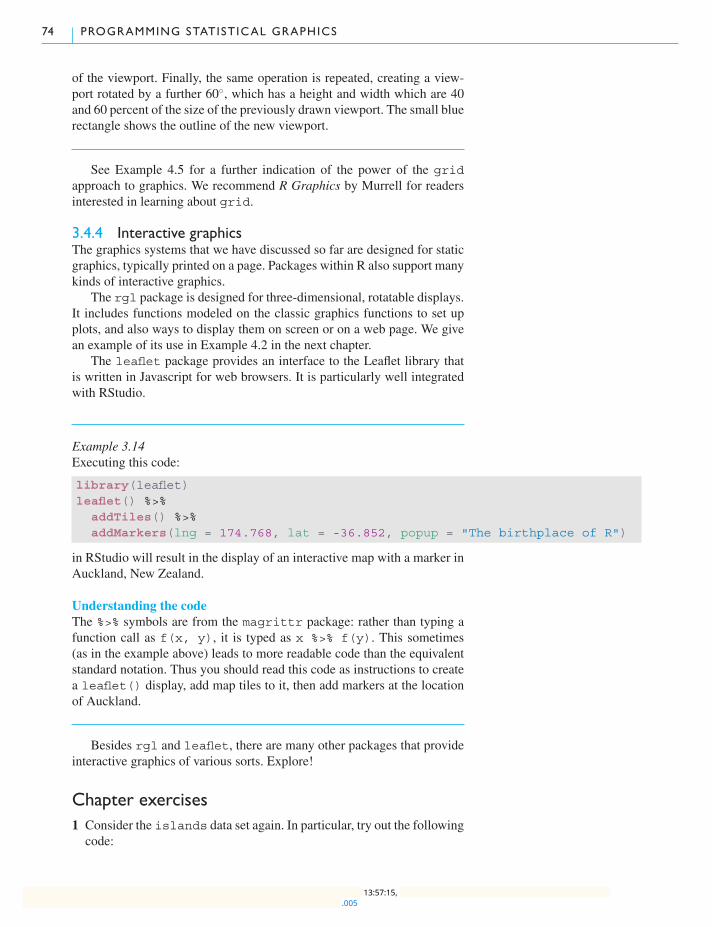
74 PROGRAMMING STATISTICAL GRAPHICS
of the viewport. Finally, the same operation is repeated, creating a view-port rotated by a further 60◦, which has a height and width which are 40and 60 percent of the size of the previously drawn viewport. The small bluerectangle shows the outline of the new viewport.
See Example 4.5 for a further indication of the power of the gridapproach to graphics. We recommend R Graphics by Murrell for readersinterested in learning about grid.
3.4.4 Interactive graphicsThe graphics systems that we have discussed so far are designed for staticgraphics, typically printed on a page. Packages within R also support manykinds of interactive graphics.
The rgl package is designed for three-dimensional, rotatable displays.It includes functions modeled on the classic graphics functions to set upplots, and also ways to display them on screen or on a web page. We givean example of its use in Example 4.2 in the next chapter.
The leaflet package provides an interface to the Leaflet library thatis written in Javascript for web browsers. It is particularly well integratedwith RStudio.
Example 3.14Executing this code:
library(leaflet)leaflet() %>%
addTiles() %>%addMarkers(lng = 174.768, lat = -36.852, popup = "The birthplace of R")
in RStudio will result in the display of an interactive map with a marker inAuckland, New Zealand.
Understanding the codeThe %>% symbols are from the magrittr package: rather than typing afunction call as f(x, y), it is typed as x %>% f(y). This sometimes(as in the example above) leads to more readable code than the equivalentstandard notation. Thus you should read this code as instructions to createa leaflet() display, add map tiles to it, then add markers at the locationof Auckland.
Besides rgl and leaflet, there are many other packages that provideinteractive graphics of various sorts. Explore!
Chapter exercises1 Consider the islands data set again. In particular, try out the following
code:
.00513:57:15,

CHAPTER EXERCISES 75
hist(log(islands,10), breaks = "Scott", axes = FALSE, xlab = "area",main = "Histogram of Landmass Areas")
axis(1, at = 1:5, labels = 10ˆ(1:5))axis(2)box()
(a) Explain what is happening at each step of the above code.(b) Add a subtitle to the plot, such as “Base-10 Log-Scale.”(c) Modify the code to incorporate the use of the Sturges rule in place
of the Scott rule. In this case, you will need to use the round()function to ensure that excessive numbers of digits are not used inthe axis labels.
2 Consider the pressure data frame again.(a) Plot pressure against temperature, and use the following com-
mand to pass a curve through these data:
curve((0.168 + 0.007*x)ˆ(20/3), from = 0, to = 400, add = TRUE)
(b) Now, apply the power transformation y3/20 to the pressure data val-ues. Plot these transformed values against temperature. Is a linearor nonlinear relationship evident now? Use the abline() functionto pass a straight line through the points. (You need an intercept andslope for this – see the previous part of this question to obtain appro-priate values.)
(c) Add a suitable title to the graph.(d) Re-do the above plots, but use themfrow() function to display them
in a 2 × 1 layout on the graphics page. Repeat once again using a1 × 2 layout.
3 Use the xyplot() function to display the orange tree data in a sequenceof five panels, one panel for each tree.
.00513:57:15,

4
Programming with R
Programming involves writing relatively complex systems of instructions.There are two broad styles of programming: the imperative style (used inR, for example) involves stringing together instructions telling the com-puter what to do. The declarative style (used in HTML in web pages, forexample) involves writing a description of the end result, without givingthe details about how to get there. Within each of these broad styles, thereare many subdivisions, and a given program may involve aspects of severalof them. For example, R programs may be procedural (describing whatsteps to take to achieve a task), modular (broken up into self-containedpackages), object-oriented (organized to describe operations on complexobjects), and/or functional (organized as a collection of functions whichdo specific calculations without having external side-effects), among otherpossibilities. In this book we will concentrate on the procedural aspects ofprogramming.
As described in Chapter 1, R statements mainly consist of expressionsto be evaluated. Most programs are very repetitive, but the amount of rep-etition depends on the input. In this chapter we start by describing sev-eral flow control statements that control how many times statements arerepeated. The remainder of the chapter gives advice on how to design anddebug programs.
4.1 Flow control
4.1.1 The for() loopOne of the goals of this book is to introduce stochastic simulation. Simu-lations are often very repetitive: we want to see patterns of behaviour, notjust a single instance.
The for() statement allows one to specify that a certain operationshould be repeated a fixed number of times.
Syntax
for (name in vector) { commands }
.00613:58:48,

4 .1 FLOW CONTROL 77
This sets a variable called name equal to each of the elements ofvector, in sequence. For each value, whatever commands are listedwithinthe curly braces will be performed. The curly braces serve to group the com-mands so that they are treated by R as a single command. If there is onlyone command to execute, the braces are not needed.
Example 4.1The factorial n! counts howmanyways n different objects could be ordered.It is defined as
n! = 1 · 2 · 3 · · · (n− 1) · n.One way to calculate it would be to use a for() statement. For example,we could find the value of 100! using the code
n <- 100result <- 1for (i in 1:n)
result <- result * iresult
## [1] 9.332622e+157
Understanding the codeThe first line sets a variable named n to 100, and the second line initializesresult to 1, i.e. a product with no terms. The third line starts the for()statement: the variable i will be set to the values 1, 2,…, n in succession.Line 4 multiplies result by i in each of those steps, and the final lineprints it.
There is also a factorial() function built into R; it is much fasterthan the for() loop. But in many cases, you will want to write your ownloops.
Example 4.2In the 1960s, IBM sold a large computer called the System/360. (We domean large: each computer filled a room.) Some programs needed unpre-dictable numbers, so they used the following scheme (called RANDU).
� Start with an odd integer x between 1 and 231 − 1 inclusive.� Multiply it by 65539, and take the remainder when dividing by 231.(These numbers have particularly simple binary representations, so theseoperations are very fast.) This gives a new value for x.
� Repeat to generate a somewhat unpredictable sequence of numbers.Divide them by 231 to put them on the scale from 0 to 1.
We can implement RANDU in a for loop. Suppose we want 1000 unpre-dictable numbers:
.00613:58:48,

78 PROGRAMMING WITH R
●●
●
●
●
●
●
●●
●
●
●
●
●
●
●
●
●
●
●
●
●
●
●
●●
●
●
●●
●
●●●
●
●
●
●●
●
●
●
●
●
●
●
●
●
●
●
●●
●
●●
●
●
●
●
●
●
●
●
●
●
●●
●
●
●
●
●
●
●
●
●
●
●
●
●
●●
●●
●
●
●
●
●
●●
●
●
●
●
●
●
●
●●
●
●
●
●
●
●●
●
●●
●
●●
●●
●
●
●
●
●
●
●
●
●
●
●
●
●
●
●
●
●
●
●
●●
●
●
●
●
●●●●
●
●
●
●
●
●
●
●
●
●
●
●
●
●
●
●
●
●
●
●
●
●
●
●
●
●
●
●
●
●
●
●
●
●
●
●
●
●
●
●
●
●
●
●
●
●
●
●
●
●●
●
●
●
●
●
●
●
●
●
●
●
●
●
●
●
●
●●●
●
●
●
●
●
●
●
●●●
●
●
●
●
●
●
●●
●
●
●
●
●
●
●
●
●
●
●
●
●
●
●
●●●
●
●
●
●
●
●
●
●
●
●
●
●
●
●
●
●
●●
●
●
●
●
●
●
●
●
●
●●
●
●
●●
●
●●
●
●
●
●
●
●
●
●
●
●
●
●●
●
●
●
●
●
●
●
●
●
●
●
●
●●
●
●
●
●
●
●
●
●
●
●
●
●
●
●
●
●
●
●
●
●
●
●
●
●
●
●
●
●
●
●
●
●
●
●
●
●
●
●
●
●
●
●
●
●
●
●
●
●
●
●●
●
●
●
●
●
●●
●
●
●
●
●
●
●
●
●
●
●
●
●
●
●
●
●
●
●
●
●
●
●
●
●
●
●●
●●
●
●
●
●
●
●
●
●
●
●
●
●●●
●●
●
●
●
●
●
●
●
●
●
●
●
●
●
●
●
●
●
●
●
●
●●
●
●
●●
●
●
●
●
●
●
●
●
●
●
●
●
●●
●
●
●
●
●
●●
●
●
●
●
●
●●
●
●
●
●
●
●
●
●
●
●●
●
●
●
●
●
●
●
●
●
●
●
●
●●●●
●
●
●
●
●
●
●
●
●
●●
●
●
●
●
●
●●
●
●
●
●
●
●
●●
●
●
●
●
●
●
●
●
●
●●
●
●
●
●
●
●
●
●
●
●
●
●
●
●
●
●
●
●
●
●
●
●
●
●
●
●
●
●●
●
●
●
●
●
●●
●
●
●
●
●●
●
●
●
●●
●
●
●●
●
●
●
●
●
●
●
●
●
●
●●
●
●
●
●
●
●
●
●
●
●
●
●
●
●
●
●
●
●
●
●
●
●
●
●
●
●●
●
●
●
●
●
●
●
●●
●
●
●
●
●
●
●
●
●
●
●
●
●●
●●
●
●
●
●
●
●
●
●
●
●
●
●
●
●
●
●
●
●●
●
●
●
●●
●
●
●
●●
●
●
●
●
●
●
●
●
●
●
●
●
●
●●
●
●
●
●
●
●
●
●
●
●
●
●
●●
●
●
●
●
●
●
●
●
●
●
●
●
●
●
●●
●
●
●
●
●
●
●●
●
●
●
●●
●
●●●●
●
●
●●
●
●
●
●
●
●
●
●
●
●
●
●
●
●
●
●
●
●
●
●
●
●
●
●
●●
●
●
●
●
●
●
●
●
●
●
●
●
●
●
●
●
●
●●
●
●
●
●
●
●
●
●●●
●
●
●
●●
●
●
●
●
●●
●
●
●
●
●
●
●
●
●●
●●
●
●
●
●
●
●
●●
●
●
●
●
●
●
●
●●
●
●
●●●
●
●
●
●
●
●
●
●
●
●
●
●
●
●
●
●●
●
●
●
●
●●
●
●
●
●●
●
●
●
●
●
●
●
●
●
●
●
●
●
●
●
●
●
●
●
●
●
●
●
●
●
●
●
●
●
●
●
●
●
●
●
●
●
●
●
●
●
●
●
●
●
●
●
●
●
●
●
●
●
●
●
●
●
●
●
●
●
●
●
●●
●
●●
●
●
●
●
●
●
●
●
●
●
●
●
●
●
●
●
●
●
●
●
●
●
●
●
●●●
●●
●
●
●
●
●
●
●
●●
●
●
●
●
●
●
●●●
●
●
●
●
●
●
●●
●
●
●
0 200 400 600 800 1000
0.0
0.2
0.4
0.6
0.8
1.0
1:1000
resu
ltsFig. 4.1 One thousand valuesfrom the RANDU algorithm.
results <- numeric(1000)x <- 123for (i in 1:1000) {
x <- (65539*x) %% (2ˆ31)results[i] <- x / (2ˆ31)
}
Understanding the codeIn the first line, we set up a vector to hold the results. The second line setsa “seed” value. The for() loop in lines 3–6 first updates x, then divides itby 231 and stores the result in the result vector. This is done for entries 1 to1000.
We can plot these numbers, and it appears that RANDU works well(Figure 4.1):
plot(1:1000, results)
If you change the value of the seed, you will see a different pattern,and the pattern is hard to predict if you don’t know that RANDU was used.However, RANDU has a terrible flaw that was not found for several years,but is obvious with modern computer graphics: all successive triplets fallinto a small subset of the 1 by 1 by 1 cube, so if you know two successivevalues, you can make a good prediction of the next. We can use the rglpackage mentioned in Section 3.4.4 to explore it:
library(rgl)plot3d(results[1:998], results[2:999], results[3:1000])
Here we are plotting successive triplets of points in three dimensions. Ifyou do this yourself, you’ll be able to rotate the display; certain orientationsshow the pattern very strikingly. Try it!
.00613:58:48,

4 .1 FLOW CONTROL 79
Example 4.3The Fibonacci sequence is a famous sequence in mathematics. The firsttwo elements are defined as [1, 1]. Subsequent elements are defined as thesum of the preceding two elements. For example, the third element is 2 (=1 + 1), the fourth element is 3 (= 1 + 2), the fifth element is 5 (= 2 + 3),and so on.
To obtain the first 12 Fibonacci numbers in R, we can use
Fibonacci <- numeric(12)Fibonacci[1] <- Fibonacci[2] <- 1for (i in 3:12)
Fibonacci[i] <- Fibonacci[i - 2] + Fibonacci[i - 1]
Understanding the codeThe first line sets up a numeric vector of length 12 with the nameFibonacci. This vector consists of 12 zeros.
The second line updates the first two elements of Fibonacci to thevalue 1.
The third line updates the third element, fourth ele-ment, and so on according to the rule defining the Fibonaccisequence. In particular, Fibonacci[3] is assigned the value ofFibonacci[1] + Fibonacci[2], i.e. 2. Fibonacci[4] is thenassigned the latest value of Fibonacci[2] + Fibonacci[3], givingit the value 3. The for() loop updates the third through 12th elements ofthe sequence in this way.
To see all 12 values, type in
Fibonacci
## [1] 1 1 2 3 5 8 13 21 34 55 89 144
Example 4.4Suppose a car dealer promotes two options for the purchase of a new$20,000 car. The first option is for the customer to pay up front and receivea $1,000 rebate. The second option is “0%-interest financing” where thecustomer makes 20 monthly payments of $1,000 beginning in one month’stime.
Because of option 1, the effective price of the car is really $19,000,so the dealer actually is charging some interest rate i for option 2. Wecan calculate this value using the formula for the present value of anannuity:
19000 = 1000
(1 − (1 + i)−20
i
).
.00613:58:48,

80 PROGRAMMING WITH R
By multiplying both sides of this equation by i and dividing by 19,000, weget the form of a fixed-point problem:1 1 A fixed-point problem arises when we
want to solve an equation of the formx = f (x), for some function f (x). Notethat the unknown value is on both sidesof the equation.
i = (1 − (1 + i)−20)/19.
By taking an initial guess for i and plugging it into the right side of thisequation, we can get an “updated” value for i on the left. For example, ifwe start with i = 0.006, then our update is
i = (1 − (1 + 0.006)−20)/19 = 0.00593.
By plugging this updated value into the right-hand side of the equationagain, we get a new update:
i = (1 − (1 + 0.00593)−20)/19 = 0.00586.
This kind of fixed-point iteration usually requires many iterations beforewe can be confident that we have the solution to the fixed-point equation.Here is R code to work out the solution after 1000 iterations:
i <- 0.006for (j in 1:1000) {
i <- (1 - (1 + i)ˆ(-20)) / 19}i
## [1] 0.004935593
Example 4.5The for() loop can be used in the programming of graphics. Figure 4.2illustrates its use in the repeated pushing of viewports, in the context of gridgraphics. In this case, 100 viewports are pushed, each has height and widthwhich are 90% of the height and width of the previous viewport, and eachis positioned slightly off-center, at the point (0.46, 0.5) relative to the pre-viously pushed viewport. Also, each viewport has been rotated by a grow-ing number of degrees, starting at 1, and increasing by 1, at each iteration.Circles having diameter equal to the height of the current viewport aredrawn at each iteration. The resulting pattern indicates the kind of complexresults that can be obtained from the grid approach to graphics, using onlya few lines of code.
library(grid)for (i in 1:100) {
vp <- viewport(x = .46, h = .9, w = .9, angle = i)pushViewport(vp)grid.circle()
}
.00613:58:48,
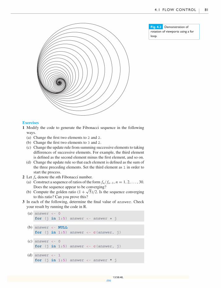
4 .1 FLOW CONTROL 81
Fig. 4.2 Demonstration ofrotation of viewports using a forloop.
Exercises1 Modify the code to generate the Fibonacci sequence in the followingways.(a) Change the first two elements to 2 and 2.(b) Change the first two elements to 3 and 2.(c) Change the update rule from summing successive elements to taking
differences of successive elements. For example, the third elementis defined as the second element minus the first element, and so on.
(d) Change the update rule so that each element is defined as the sum ofthe three preceding elements. Set the third element as 1 in order tostart the process.
2 Let fn denote the nth Fibonacci number.(a) Construct a sequence of ratios of the form fn/ fn−1, n = 1, 2, . . . , 30.
Does the sequence appear to be converging?(b) Compute the golden ratio (1 + √
5)/2. Is the sequence convergingto this ratio? Can you prove this?
3 In each of the following, determine the final value of answer. Checkyour result by running the code in R.
(a) answer <- 0for (j in 1:5) answer <- answer + j
(b) answer <- NULLfor (j in 1:5) answer <- c(answer, j)
(c) answer <- 0for (j in 1:5) answer <- c(answer, j)
(d) answer <- 1for (j in 1:5) answer <- answer * j
.00613:58:48,

82 PROGRAMMING WITH R
(e) answer <- 3for (j in 1:15) answer <- c(answer, (7 * answer[j]) %% 31)
Inspect this last sequence of numbers. If you did not know therule used to determine this sequence, would you be able to predictsuccessive elements?
4 Refer to the car dealer promotion example in this section. Calculate thefirst 20 updates of the interest rate i, starting with i = 0.006. Repeat witha starting value of i = 0.005, and with a starting value of i = 0.004.Based on these observations, what is the true value of i (up to 5 digitaccuracy)?
5 Use a fixed-point iteration to determine the solution (in [0, 1]) of theequation x = cos(x). Use a starting value of 0.5. How many iterationsdoes it take before you have an answer which is accurate in the first 2digits? . . . in the first 3 digits? . . . in the first 4 digits? What happens ifyou change the starting value to 0.7? . . . to 0.0?
6 Repeat the previous question, but using the equation x = 1.5 cos(x). (Thesolution is near x = 0.9148565.)(a) Does the fixed-point iteration converge? If not, modify the equation
so that x = cos(x)/30 + 44x/45. Does the iteration converge now?(b) Can you show that the solutions to these two equations are the same?(c) Compute the absolute value of the derivative of 1.5 cos(x) and of
cos(x)/30 + 44x/45. There is a theorem in numerical analysis whichsays that if this quantity is less than 1, then the fixed-point iterationwill converge if the starting guess is close enough to the solution.Does this explain the behavior that you observed in part (a)?
7 Refer to the grid graphics example. Modify the code so that rectanglesare created instead of circles. Center the rectangles at (.5, .5) instead of(.46, .5), and set the angle of rotation to 0 instead of i. Comment on theresult.
4.1.2 The if() statementEarlier, we learned about logical vectors and relational operators. The sub-scripting device is a powerful way to perform different operations on differ-ent parts of vectors. The if() statement allows us to control which state-ments are executed, and sometimes this is more convenient.
Syntaxif (condition) {commands when TRUE}if (condition) {commands when TRUE} else {commands when FALSE}
This statement causes a set of commands to be invoked if conditionevaluates to TRUE. The else part is optional, and provides an alternativeset of commands which are to be invoked in case the logical variable isFALSE. Be careful how you type this. If you put the else part on a newline, you may see something like this:
if (condition) {# do TRUE
}
.00613:58:48,
4 .1 FLOW CONTROL 83
else {^## Error: unexpected ’else’ in "else"
R executed the first three lines before you entered the else. This meant itwasn’t expecting an else, and it signalled an error.2 To avoid this problem, 2 If these lines had appeared within a
block of commands in curly braces, theywouldn’t have triggered an error,because R would collect all the linesbefore starting to act on any of them: butit is still a good idea to avoid thisambiguity.
a common convention for typing if ... else is to put the else on thesame line as the previous closing brace:
if (condition) {# do TRUE
} else {# do FALSE
}
This way it is very clear that the statement is incomplete until the very end.R also allows numerical values to be used as the value of condition.
These are converted to logical values using the rule that zero becomesFALSE, and any other value becomes TRUE.
Missing values are not allowed for the condition, and will trigger anerror.
Example 4.6A simple example:
x <- 3if (x > 2) y <- 2 * x else y <- 3 * x
Since x > 2 is TRUE, y is assigned 2 * 3 = 6. If it hadn’t been true,y would have been assigned the value of 3 * x.
The if() statement is often used inside user-defined functions. Thefollowing is a typical example.
Example 4.7The correlation between two vectors of numbers is often calculated usingthe cor() function. It is supposed to give a measure of linear association.We can add a scatter plot of the data as follows.
corplot <- function(x, y, plotit) {if (plotit == TRUE) plot(x, y)cor(x, y)
}
We can apply this function to two vectors without plotting by typing
corplot(c(2, 5, 7), c(5, 6, 8), FALSE)
## [1] 0.953821
.00613:58:48,

84 PROGRAMMING WITH R
Example 4.8The function that follows is based on the sieve of Eratosthenes, the oldestknown systematic method for listing prime numbers up to a given value n.The idea is as follows: begin with a vector of numbers from 2 to n. Begin-ning with 2, eliminate all multiples of 2 which are larger than 2. Then moveto the next number remaining in the vector, in this case, 3. Now, removeall multiples of 3 which are larger than 3. Proceed through all remainingentries of the vector in this way. The entry for 4 would have been removedin the first round, leaving 5 as the next entry to work with after 3; allmultiples of 5 would be removed at the next step, and so on.
Eratosthenes <- function(n) {# Return all prime numbers up to n (based on the sieve of Eratosthenes)
if (n >= 2) {sieve <- seq(2, n)primes <- c()for (i in seq(2, n)) {
if (any(sieve == i)) {primes <- c(primes, i)sieve <- c(sieve[(sieve %% i) != 0], i)
}}return(primes)
} else {stop("Input value of n should be at least 2.")
}}
Here are some examples of the use of this function:
Eratosthenes(50)
## [1] 2 3 5 7 11 13 17 19 23 29 31 37 41 43 47
Eratosthenes(-50)
## Error in Eratosthenes(-50): Input value of n should be at least 2.
Understanding the codeThe purpose of the function is to provide all prime numbers up to the givenvalue n. The basic idea of the program is contained in the lines
sieve <- seq(2, n)primes <- c()for (i in seq(2, n)) {
if (any(sieve == i)) {primes <- c(primes, i)sieve <- sieve[(sieve %% i) != 0]
}}
.00613:58:48,

4 .1 FLOW CONTROL 85
The sieve object holds all the candidates for testing. Initially, all inte-gers from 2 through n are stored in this vector. The primes object is set upinitially empty, eventually to contain all of the primes that are less than orequal to n. The composite numbers in sieve are removed, and the primesare copied to primes.
Each integer i from 2 through n is checked in sequence to see whetherit is still in the vector. The any() function returns a TRUE if at least oneof the logical vector elements in its argument is TRUE. In the case that i isstill in the sieve vector, it must be a prime, since it is the smallest numberthat has not been eliminated yet. All multiples of i are eliminated, sincethey are necessarily composite, and i is appended to primes. The expres-sion (sieve %% i) == 0 would give TRUE for all elements of sievewhich are multiples of i; since we want to eliminate these elements andsave all other elements, we can negate this using !(sieve %% i == 0)or sieve %% i != 0. Then we can eliminate all multiples of i from thesieve vector using
sieve <- sieve[(sieve %% i) != 0]
Note that this eliminates i as well, but we have already saved it in primes.If the supplied argument n is less than 2, then the function output would
be meaningless. To avoid this, we cause an error to be triggered if a valuesmaller than 2 is supplied by the user.
Exercises1 Does the Eratosthenes() function work properly if n is not an
integer? Is an error message required in this case?2 Use the idea of the Eratosthenes() function to prove that there areinfinitely many primes. Hint: suppose all primes were less than m, andconstruct a larger value n that would not be eliminated by the sieve.
3 A twin prime is a pair of primes (x, y), such that y = x+ 2. Construct alist of all twin primes less than 1000.3 3 It has been known since ancient times
that there are infinitely many primes. Itremains a conjecture as to whether thereis an infinite set of twin primes.
4 A bank offers a guaranteed investment certificate (GIC) which pays anannual interest rate of 4% (compounded annually) if the term is 3 yearsor less, or 5% if the term is more than 3 years. Write a function whichtakes the initial investment amount, P, and the number of interest periods(i.e. years) as arguments and which returns the amount of interest earnedover the term of the GIC. That is, return I, where I = P((1 + i)n − 1).
5 Mortgage interest rates can sometimes depend on whether the mortgageterm is open or closed. Use the formula
R = Pi
1 − (1 + i)−n
to create a function to calculate amonthlymortgage paymentRwhere i isan interest rate (compounded monthly), P is the original principal, and nis the length of the term (in months). The function should take n, P, andopen as arguments. If open==TRUE, then take i = 0.005; otherwise,take i = 0.004.
.00613:58:48,
86 PROGRAMMING WITH R
4.1.3 The while() loopSometimes we want to repeat statements, but the pattern of repetition isn’tknown in advance. We need to do some calculations and keep going as longas a condition holds. The while() statement accomplishes this.
Syntaxwhile (condition) {statements}
The condition is evaluated, and if it evaluates to FALSE, noth-ing more is done. If it evaluates to TRUE the statements are executed,condition is evaluated again, and the process is repeated.
Example 4.9Suppose we want to list all Fibonacci numbers less than 300. We don’tknow beforehand how long this list is, so we wouldn’t know how to stopthe for() loop at the right time, but a while() loop is perfect:
Fib1 <- 1Fib2 <- 1Fibonacci <- c(Fib1, Fib2)while (Fib2 < 300) {
Fibonacci <- c(Fibonacci, Fib2)oldFib2 <- Fib2Fib2 <- Fib1 + Fib2Fib1 <- oldFib2
}
Understanding the codeThe central idea is contained in the lines
while (Fib2 < 300) {Fibonacci <- c(Fibonacci, Fib2)
That is, as long as the latest Fibonacci number created (in Fib2) is lessthan 300, it is appended to the growing vector Fibonacci.
Thus, we must ensure that Fib2 actually contains the updatedFibonacci number. By keeping track of the two most recently added num-bers (Fib1 and Fib2), we can do the update
Fib2 <- Fib1 + Fib2
Now Fib1 should be updated to the old value of Fib2, but that has beenoverwritten by the new value. So before executing the above line, we makea copy of Fib2 in oldFib2. After updating Fib2, we can assign the valuein oldFib2 to Fib1.
In order to start things off, Fib1, Fib2, and Fibonacci need to beinitialized. That is, within the loop, these objects will be used, so they needto be assigned sensible starting values.
.00613:58:48,

4 .1 FLOW CONTROL 87
To see the final result of the computation, type
Fibonacci
## [1] 1 1 1 2 3 5 8 13 21 34 55 89 144 233
CautionIncreasing the length of a vector element by element as inFibonacci <- c(Fibonacci, Fib2) in a for() or while()loop should be avoided if the number of such operations is likely to belarge. R will have to keep allocating new vectors, each one element longerthan the last one, and this will slow the process down substantially.
Exercises1 The variable oldFib2 isn’t strictly necessary. Rewrite the Fibonacciwhile() loop with the update of Fib1 based just on the current valuesof Fib1 and Fib2.
2 In fact, Fib1 and Fib2 aren’t necessary either. Rewrite the Fibonacciwhile() loop without using any variables except Fibonacci.
3 Determine the number of Fibonacci numbers less than 1000000.4 Recall the car dealer interest rate example in Example 4.4. Use awhile() loop to iteratively calculate the interest rate i which satisfiesthe fixed-point equation
i = (1 − (1 + i)−20)/19.
Use a starting guess of i = 0.006. Stop the calculation when two succes-sive values of the interest rate are less than 0.000001 apart.
What happens when you try other starting guesses?5 Referring to the previous exercise, modify your code so that it also com-putes the number of iterations required to get two successive values ofthe interest rate that are less than 0.000001 apart.
4.1.4 Newton’s method for root findingNewton’s method is a popular numerical method to find a root of an alge-braic equation:4 4 Alternatively, we say that it is finding
a zero of the function f (x).f (x) = 0.
If f (x) has derivative f ′(x), then the following iteration should converge toa root of the above equation if started close enough to the root.
x0 = initial guess,
xn = xn−1 − f (xn−1)
f ′(xn−1).
The idea is based on the Taylor approximation
f (xn) ≈ f (xn−1) + (xn − xn−1) f′(xn−1). (4.1)
Newton’s method is equivalent to setting f (xn) = 0 and solving for xn in(4.1). Even though (4.1) is only an approximation, we hope that the solution
.00613:58:48,
88 PROGRAMMING WITH R
xn should give a close approximation to the root. Be careful: there are manyexamples where xn will fail to converge to a root unless xn−1 is already suf-ficiently close, and some where it will fail regardless of the starting value.
Example 4.10Suppose f (x) = x3 + 2x2 − 7. Then, if x0 is close enough to one of thethree roots of this equation,
xn = xn−1 − x3n−1 + 2x2n−1 − 7
3x2 + 4x
will converge to a root.An R version of this could be implemented as follows:
x <- x0f <- xˆ3 + 2 * xˆ2 - 7tolerance <- 0.000001while (abs(f) > tolerance) {
f.prime <- 3 * xˆ2 + 4 * xx <- x - f / f.primef <- xˆ3 + 2 * xˆ2 - 7
}x
Understanding the codeWe start with x equal to x0, and evaluate f (x0). Then, as long as | f (xi)| ismore than 0.000001, we update x using Newton’s method. Notice that wedon’t need a variable i. Because Newton’s method is a recursive formulawhere the new value can be calculated from the old one, there is no needto know which iteration we are on when doing the updates.
Exercises1 The equation
x7 + 10000x6 + 1.06x5 + 10600x4 + 0.0605x3 + 605x2 + 0.0005x+ 5
has exactly one real root. How many iterations of Newton’s method arerequired to find this root if the initial guess is x = 0?
2 Use Newton’s method to find a zero of
f (x) = x4 + 3x3 − 2x2 − 7
using an initial guess of x = 1.3 Modify the above function so that it finds one of the zeros of
f (x) = cos(x) + ex
using an initial guess of x = −1.5.4 Find a minimizer of the function
f (x) = (x− 3)4 + 7(x− 2)2 + x.
.00613:58:48,
4 .1 FLOW CONTROL 89
5 How many zeros does the function
f (x) = 5x− 3
x− 1
have?What are they? Describe the behavior of Newton’s method appliedto this function if the initial guess is(a) 0.5(b) 0.75(c) 0.2(d) 1.25
6 How many zeros does the function
f (x) = (x2 − 6x+ 9)e−x
have? What are they? Describe the behaviour of Newton’s methodapplied to this function if the initial guess is(a) 3(b) 3.2(c) 2.99(d) 3.01
7 Refer to the car dealer interest rate example in Example 4.4. Use New-ton’s method to calculate the interest rate i which satisfies
i = (1 − (1 + i)−20)/19.
Use i = 0.006 as your starting guess. How many iterations are requiredfor two successive values of i to be within 0.000001 of each other?
4.1.5 The repeat loop, and the break andnext statementsSometimes we don’t want a fixed number of repetitions of a loop, and wedon’t want to put the test at the top of the loop the way it is in a while()loop. In this situation we can use a repeat loop. This loop repeats untilwe execute a break statement.
Syntaxrepeat { statements }
This causes the statements to be repeated endlessly. The statementsshould normally include a break statement, typically in the form
if (condition) break
but this is not a requirement of the syntax.The break statement causes the loop to terminate immediately. break
statements can also be used in for() and while() loops. The next state-ment causes control to return immediately to the top of the loop; it can alsobe used in any loop.
The repeat loop and the break and next statements are used rela-tively infrequently. It is usually easier to understand code when the test isclearly displayed at the top, and when that is the only exit from the loop (asin the for and while loops.) However, sometimes these statements helpto make programs clearer.
.00613:58:48,
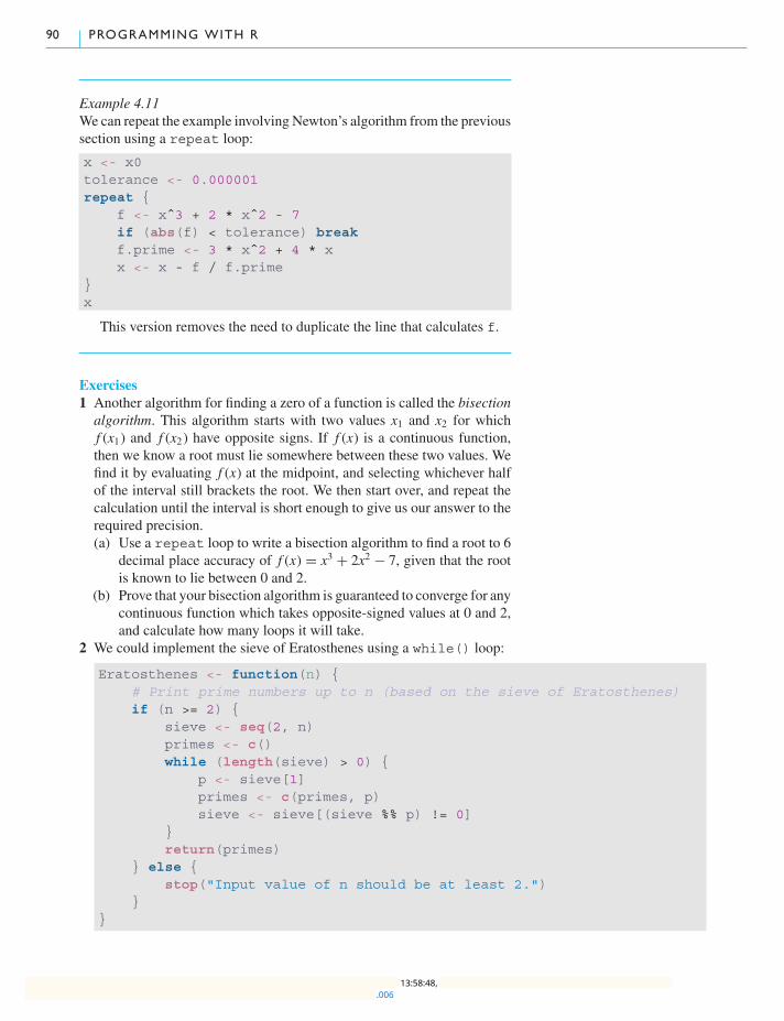
90 PROGRAMMING WITH R
Example 4.11We can repeat the example involving Newton’s algorithm from the previoussection using a repeat loop:
x <- x0tolerance <- 0.000001repeat {
f <- xˆ3 + 2 * xˆ2 - 7if (abs(f) < tolerance) breakf.prime <- 3 * xˆ2 + 4 * xx <- x - f / f.prime
}x
This version removes the need to duplicate the line that calculates f.
Exercises1 Another algorithm for finding a zero of a function is called the bisectionalgorithm. This algorithm starts with two values x1 and x2 for whichf (x1) and f (x2) have opposite signs. If f (x) is a continuous function,then we know a root must lie somewhere between these two values. Wefind it by evaluating f (x) at the midpoint, and selecting whichever halfof the interval still brackets the root. We then start over, and repeat thecalculation until the interval is short enough to give us our answer to therequired precision.(a) Use a repeat loop to write a bisection algorithm to find a root to 6
decimal place accuracy of f (x) = x3 + 2x2 − 7, given that the rootis known to lie between 0 and 2.
(b) Prove that your bisection algorithm is guaranteed to converge for anycontinuous function which takes opposite-signed values at 0 and 2,and calculate how many loops it will take.
2 We could implement the sieve of Eratosthenes using a while() loop:
Eratosthenes <- function(n) {# Print prime numbers up to n (based on the sieve of Eratosthenes)if (n >= 2) {
sieve <- seq(2, n)primes <- c()while (length(sieve) > 0) {
p <- sieve[1]primes <- c(primes, p)sieve <- sieve[(sieve %% p) != 0]
}return(primes)
} else {stop("Input value of n should be at least 2.")
}}
.00613:58:48,
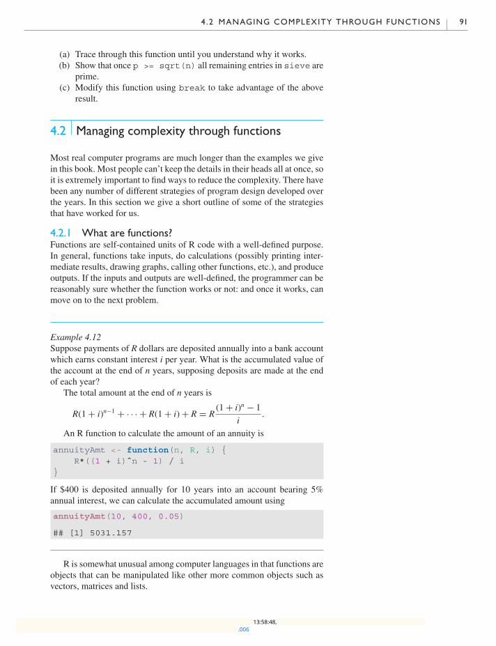
4 .2 MANAGING COMPLEXITY THROUGH FUNCTIONS 91
(a) Trace through this function until you understand why it works.(b) Show that once p >= sqrt(n) all remaining entries in sieve are
prime.(c) Modify this function using break to take advantage of the above
result.
4.2 Managing complexity through functions
Most real computer programs are much longer than the examples we givein this book. Most people can’t keep the details in their heads all at once, soit is extremely important to find ways to reduce the complexity. There havebeen any number of different strategies of program design developed overthe years. In this section we give a short outline of some of the strategiesthat have worked for us.
4.2.1 What are functions?Functions are self-contained units of R code with a well-defined purpose.In general, functions take inputs, do calculations (possibly printing inter-mediate results, drawing graphs, calling other functions, etc.), and produceoutputs. If the inputs and outputs are well-defined, the programmer can bereasonably sure whether the function works or not: and once it works, canmove on to the next problem.
Example 4.12Suppose payments of R dollars are deposited annually into a bank accountwhich earns constant interest i per year. What is the accumulated value ofthe account at the end of n years, supposing deposits are made at the endof each year?
The total amount at the end of n years is
R(1 + i)n−1 + · · · + R(1 + i) + R = R(1 + i)n − 1
i.
An R function to calculate the amount of an annuity is
annuityAmt <- function(n, R, i) {R*((1 + i)ˆn - 1) / i
}
If $400 is deposited annually for 10 years into an account bearing 5%annual interest, we can calculate the accumulated amount using
annuityAmt(10, 400, 0.05)
## [1] 5031.157
R is somewhat unusual among computer languages in that functions areobjects that can be manipulated like other more common objects such asvectors, matrices and lists.
.00613:58:48,
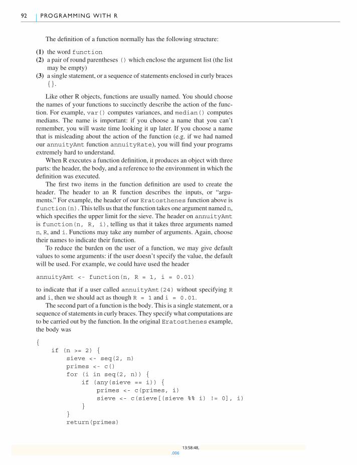
92 PROGRAMMING WITH R
The definition of a function normally has the following structure:
(1) the word function(2) a pair of round parentheses ()which enclose the argument list (the list
may be empty)(3) a single statement, or a sequence of statements enclosed in curly braces
{}.
Like other R objects, functions are usually named. You should choosethe names of your functions to succinctly describe the action of the func-tion. For example, var() computes variances, and median() computesmedians. The name is important: if you choose a name that you can’tremember, you will waste time looking it up later. If you choose a namethat is misleading about the action of the function (e.g. if we had namedour annuityAmt function annuityRate), you will find your programsextremely hard to understand.
When R executes a function definition, it produces an object with threeparts: the header, the body, and a reference to the environment in which thedefinition was executed.
The first two items in the function definition are used to create theheader. The header to an R function describes the inputs, or “argu-ments.” For example, the header of our Eratosthenes function above isfunction(n). This tells us that the function takes one argument named n,which specifies the upper limit for the sieve. The header on annuityAmtis function(n, R, i), telling us that it takes three arguments namedn, R, and i. Functions may take any number of arguments. Again, choosetheir names to indicate their function.
To reduce the burden on the user of a function, we may give defaultvalues to some arguments: if the user doesn’t specify the value, the defaultwill be used. For example, we could have used the header
annuityAmt <- function(n, R = 1, i = 0.01)
to indicate that if a user called annuityAmt(24) without specifying Rand i, then we should act as though R = 1 and i = 0.01.
The second part of a function is the body. This is a single statement, or asequence of statements in curly braces. They specify what computations areto be carried out by the function. In the original Eratosthenes example,the body was
{if (n >= 2) {
sieve <- seq(2, n)primes <- c()for (i in seq(2, n)) {
if (any(sieve == i)) {primes <- c(primes, i)sieve <- c(sieve[(sieve %% i) != 0], i)
}}return(primes)
.00613:58:48,
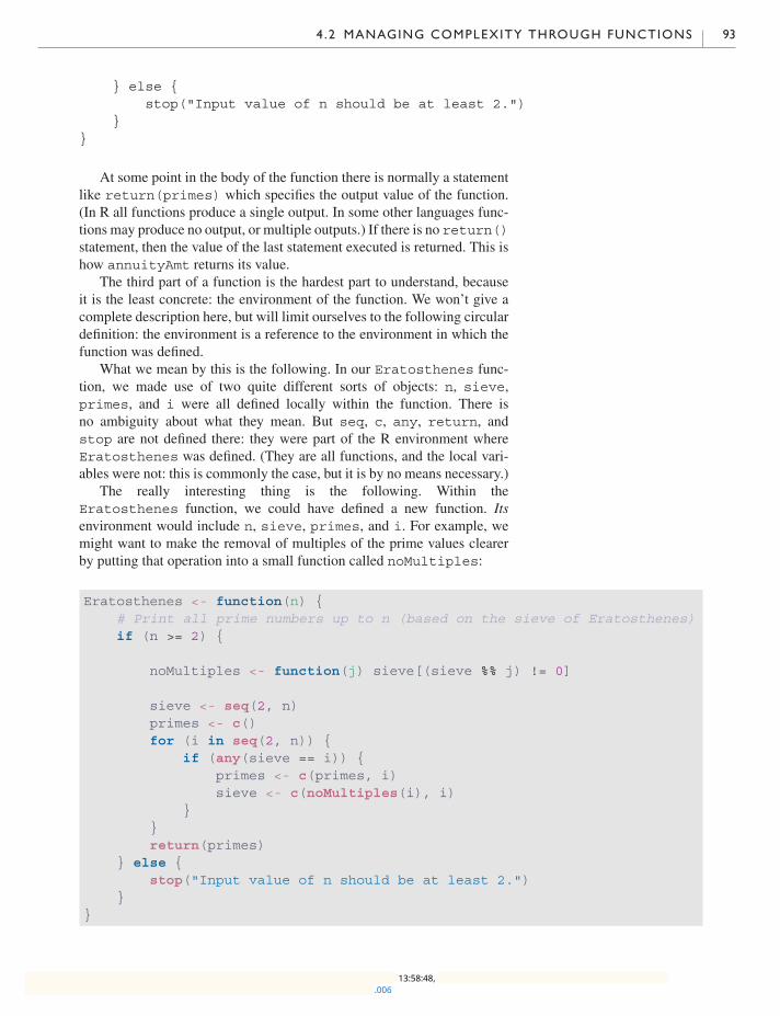
4 .2 MANAGING COMPLEXITY THROUGH FUNCTIONS 93
} else {stop("Input value of n should be at least 2.")
}}
At some point in the body of the function there is normally a statementlike return(primes) which specifies the output value of the function.(In R all functions produce a single output. In some other languages func-tions may produce no output, or multiple outputs.) If there is no return()statement, then the value of the last statement executed is returned. This ishow annuityAmt returns its value.
The third part of a function is the hardest part to understand, becauseit is the least concrete: the environment of the function. We won’t give acomplete description here, but will limit ourselves to the following circulardefinition: the environment is a reference to the environment in which thefunction was defined.
What we mean by this is the following. In our Eratosthenes func-tion, we made use of two quite different sorts of objects: n, sieve,primes, and i were all defined locally within the function. There isno ambiguity about what they mean. But seq, c, any, return, andstop are not defined there: they were part of the R environment whereEratosthenes was defined. (They are all functions, and the local vari-ables were not: this is commonly the case, but it is by no means necessary.)
The really interesting thing is the following. Within theEratosthenes function, we could have defined a new function. Itsenvironment would include n, sieve, primes, and i. For example, wemight want to make the removal of multiples of the prime values clearerby putting that operation into a small function called noMultiples:
Eratosthenes <- function(n) {# Print all prime numbers up to n (based on the sieve of Eratosthenes)if (n >= 2) {
noMultiples <- function(j) sieve[(sieve %% j) != 0]
sieve <- seq(2, n)primes <- c()for (i in seq(2, n)) {
if (any(sieve == i)) {primes <- c(primes, i)sieve <- c(noMultiples(i), i)
}}return(primes)
} else {stop("Input value of n should be at least 2.")
}}
.00613:58:48,
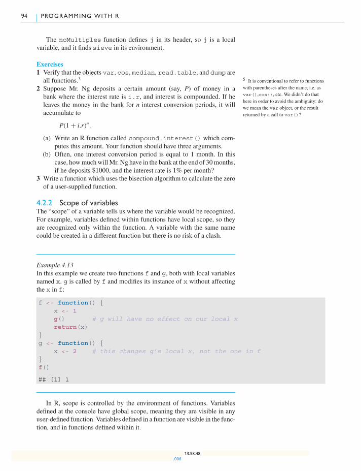
94 PROGRAMMING WITH R
The noMultiples function defines j in its header, so j is a localvariable, and it finds sieve in its environment.
Exercises1 Verify that the objects var, cos, median, read.table, and dump are
all functions.5 5 It is conventional to refer to functionswith parentheses after the name, i.e. asvar(),cos(), etc. We didn’t do thathere in order to avoid the ambiguity: dowe mean the var object, or the resultreturned by a call to var()?
2 Suppose Mr. Ng deposits a certain amount (say, P) of money in abank where the interest rate is i.r, and interest is compounded. If heleaves the money in the bank for n interest conversion periods, it willaccumulate to
P(1 + i.r)n.
(a) Write an R function called compound.interest() which com-putes this amount. Your function should have three arguments.
(b) Often, one interest conversion period is equal to 1 month. In thiscase, howmuchwillMr. Ng have in the bank at the end of 30months,if he deposits $1000, and the interest rate is 1% per month?
3 Write a function which uses the bisection algorithm to calculate the zeroof a user-supplied function.
4.2.2 Scope of variablesThe “scope” of a variable tells us where the variable would be recognized.For example, variables defined within functions have local scope, so theyare recognized only within the function. A variable with the same namecould be created in a different function but there is no risk of a clash.
Example 4.13In this example we create two functions f and g, both with local variablesnamed x. g is called by f and modifies its instance of x without affectingthe x in f:
f <- function() {x <- 1g() # g will have no effect on our local xreturn(x)
}g <- function() {
x <- 2 # this changes g’s local x, not the one in f}f()
## [1] 1
In R, scope is controlled by the environment of functions. Variablesdefined at the console have global scope, meaning they are visible in anyuser-defined function. Variables defined in a function are visible in the func-tion, and in functions defined within it.
.00613:58:48,
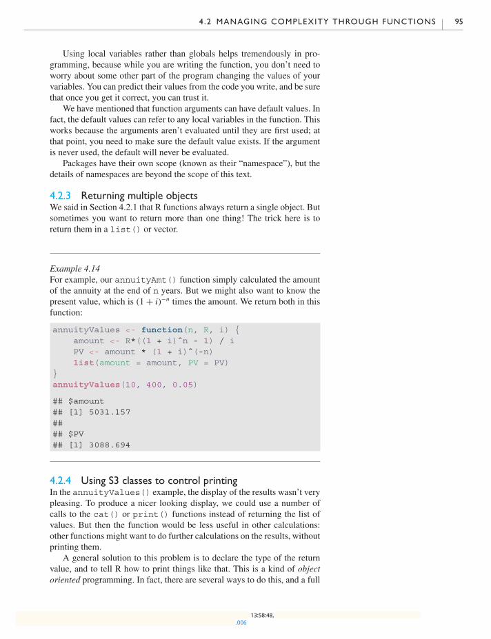
4 .2 MANAGING COMPLEXITY THROUGH FUNCTIONS 95
Using local variables rather than globals helps tremendously in pro-gramming, because while you are writing the function, you don’t need toworry about some other part of the program changing the values of yourvariables. You can predict their values from the code you write, and be surethat once you get it correct, you can trust it.
We have mentioned that function arguments can have default values. Infact, the default values can refer to any local variables in the function. Thisworks because the arguments aren’t evaluated until they are first used; atthat point, you need to make sure the default value exists. If the argumentis never used, the default will never be evaluated.
Packages have their own scope (known as their “namespace”), but thedetails of namespaces are beyond the scope of this text.
4.2.3 Returning multiple objectsWe said in Section 4.2.1 that R functions always return a single object. Butsometimes you want to return more than one thing! The trick here is toreturn them in a list() or vector.
Example 4.14For example, our annuityAmt() function simply calculated the amountof the annuity at the end of n years. But we might also want to know thepresent value, which is (1 + i)−n times the amount. We return both in thisfunction:
annuityValues <- function(n, R, i) {amount <- R*((1 + i)ˆn - 1) / iPV <- amount * (1 + i)ˆ(-n)list(amount = amount, PV = PV)
}annuityValues(10, 400, 0.05)
## $amount## [1] 5031.157#### $PV## [1] 3088.694
4.2.4 Using S3 classes to control printingIn the annuityValues() example, the display of the results wasn’t verypleasing. To produce a nicer looking display, we could use a number ofcalls to the cat() or print() functions instead of returning the list ofvalues. But then the function would be less useful in other calculations:other functions might want to do further calculations on the results, withoutprinting them.
A general solution to this problem is to declare the type of the returnvalue, and to tell R how to print things like that. This is a kind of objectoriented programming. In fact, there are several ways to do this, and a full
.00613:58:48,
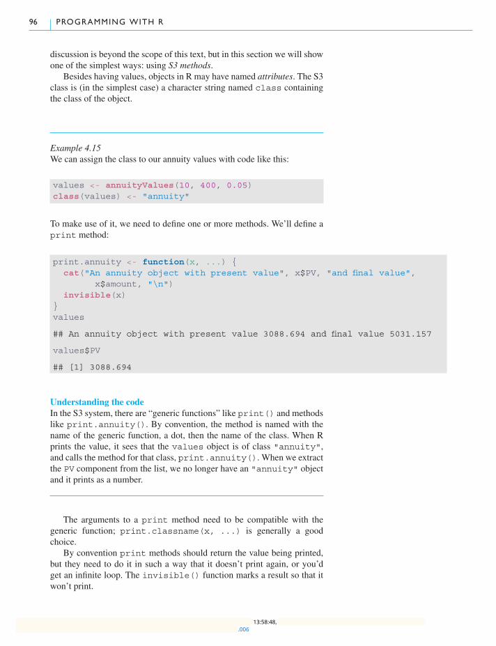
96 PROGRAMMING WITH R
discussion is beyond the scope of this text, but in this section we will showone of the simplest ways: using S3 methods.
Besides having values, objects in R may have named attributes. The S3class is (in the simplest case) a character string named class containingthe class of the object.
Example 4.15We can assign the class to our annuity values with code like this:
values <- annuityValues(10, 400, 0.05)class(values) <- "annuity"
To make use of it, we need to define one or more methods. We’ll define aprint method:
print.annuity <- function(x, ...) {cat("An annuity object with present value", x$PV, "and final value",
x$amount, "\n")invisible(x)
}values
## An annuity object with present value 3088.694 and final value 5031.157
values$PV
## [1] 3088.694
Understanding the codeIn the S3 system, there are “generic functions” like print() and methodslike print.annuity(). By convention, the method is named with thename of the generic function, a dot, then the name of the class. When Rprints the value, it sees that the values object is of class "annuity",and calls the method for that class, print.annuity(). When we extractthe PV component from the list, we no longer have an "annuity" objectand it prints as a number.
The arguments to a print method need to be compatible with thegeneric function; print.classname(x, ...) is generally a goodchoice.
By convention print methods should return the value being printed,but they need to do it in such a way that it doesn’t print again, or you’dget an infinite loop. The invisible() function marks a result so that itwon’t print.
.00613:58:48,

4 .4 MISCELLANEOUS PROGRAMMING TIPS 97
4.3 The replicate() function
Section 4.1 was about flow control. The for(), while(), and repeatloops allow increasing flexibility in looping. In this section we describe astep in the opposite direction: the replicate() function.
The replicate() function is something like a for() loop, with afew differences. For one thing, the syntax looks like a function call:
replicate(n, { statements })
This says to evaluate the statements n times. Another difference is that itreturns the result of each evaluation, whereas the for() loop does notreturn the values. If the value in each step is a vector, it returns a matrix:
replicate(5, 1:3)
## [,1] [,2] [,3] [,4] [,5]## [1,] 1 1 1 1 1## [2,] 2 2 2 2 2## [3,] 3 3 3 3 3
Finally, there’s a difference in scoping. Changes made within a for() loophave global scope, but thereplicate() function evaluates the statementsin a local scope, much as a function evaluates its body. Thus the followingimplementation of the RANDU algorithm gives repetitive output:
x <- 123replicate(10, {
x <- (65539*x) %% (2ˆ31)x / (2ˆ31)
})
## [1] 0.003753834 0.003753834 0.003753834 0.003753834 0.003753834## [6] 0.003753834 0.003753834 0.003753834 0.003753834 0.003753834
We’ll see examples in Chapter 5 where these properties are very convenientin simulations of random processes.
4.4 Miscellaneous programming tips
4.4.1 Always edit code in the editor, not in the consoleSometimes we make errors when we write code. It is easy in the R consoleto use the up-arrow to retrieve a previous command, change it, and then runit again. However, we strongly discourage this style of programming.
A much better style is to write your commands in the editor, and runthem from there. If you get it wrong, fix it in the editor and try again. Thisway you work towards having a script that does a long calculation correctly,rather than ending up with a console history containing all of your errors.It is also easier to start from the beginning and re-run many lines, if theyare all in the editor.
.00613:58:48,
98 PROGRAMMING WITH R
4.4.2 Documentation using #The # symbol is a simple way of inserting comments such as titlesand descriptions into R functions and scripts. R ignores all text from the# character to the end of the line.
It is good practice to add a title and short description to any functionthat you create, so that you and other users can be reminded later of thepurpose of the function. It is surprising how easy it is to forget the purposeof a function created only a few weeks or months ago.
It is also sometimes useful to describe what a particular line of codedoes. This is especially useful when an obscure command has been used.
When working in RStudio, the “Code” menu offers several entries tomake this very easy. You can use “Code | Comment/Uncomment lines” toadd (or remove) comment markers from a range of lines. If your commentstake up too much space on a line (or too little), you can “Code | ReflowComment” to get more evenly spaced lines.
4.4.3 Neatness counts!When first programming, it is tempting to think that the only goal is to get aprogram that works. When it gives the expected result in a few tests, you’redone. In Section 4.6.1 we’ll talk about ways to improve your testing. Butmore importantly, you want to write code that “obviously” works, and thatmeans writing clearly, and formatting your code neatly. In this section we’llgive some tips for formatting.
1. Use spacing and line breaks to make long expressions easier to read. It’sgenerally a good idea to put spaces around most operators in expres-sions, and to break long expressions into multiple lines. For example, inR the expressions
x1<-a+b+cy12< -a+b+c
are confusingly similar, but very different: the first one assigns the valueof a + b + c to x1, while the second compares y12 to -a + b + c.If we add some spaces around the assignment, comparison, and additionoperators (but not the negative sign), they’ll be easier to read:
x1 <- a + b + cy12 < -a + b + c
We added two spaces after x1 so that the very similar expressions on theright would line up, making it easier to spot the differences. With thisformatting the differences stand out, and if they were not intentionalthey would be easy to fix.
2. Indent according to the logical organization of your program. In Sec-tions 4.1 and 4.2 we described flow control and functions, both ways tologically organize your program. These techniques help make your pro-gram more understandable, but if the reader doesn’t see them the wayR does, they can be a source of a huge amount of confusion. We thusmake the following recommendation regarding indentation: put open-ing braces "{" at the end of a line, and closing ones "}" at the start
.00613:58:48,

4 .4 MISCELLANEOUS PROGRAMMING TIPS 99
of a line, indented equally to the line that started the block. Indent lineswithin the block consistently, e.g. by two or four spaces. For example,on page 93 we defined the complex function Eratosthenes contain-ing if statements and for loops in its body. We used four spaces ofindentation to indicate each additional level of nesting, and so it is clearwhere the body starts and ends, and the scope of each flow control state-ment. Putting the closing brace at the end of the line has the additionalbeneficial effect in R of preventing a syntax error when the if statementis complete before the else statement is seen.
3. Use informative and consistently formatted variable names. Once youare writing a long program, it becomes hard to remember what the vari-ables do. Mathematical style is to use single letters for variables (per-haps with different typefaces, or accents, superscripts, or subscripts),but this doesn’t work in programming: you are generally restricted toa single typeface without any modifications. This makes it importantto use longer names for things, for example wheelRadius instead ofr1. It is also important to adopt a consistent style for names contain-ing two or more words. We like camel case as in wheelRadius, butothers advocate separators such as wheel_radius. Unfortunately thenames of R functions are inconsistent in this so we can’t give a singlerecommendation, but you should aim to be consistent within your ownprograms.
Exercises1 Compute 10!, 50!, 100!, and 1000!.2 (a) Using fix() and factorial(), create a function which computes
the binomial coefficient(n
m
).
(b) Compute(42
),(5020
), and
(50002000
).
(c) The sum() function can be used to sum up all elements of itsargument, while the log() and exp() functions take the naturallogarithm and exponential of all elements in their argument. Usethese functions to create an improved function to compute binomialcoefficients.
(d) Compute(42
),(5020
), and
(50002000
)using the improved version.
3 Refer to Exercise 2 of Section 4.2.1 in which you created a functioncalled compound.interest(). Often, the interest rate is quoted as anominal annual rate, compounded monthly. To obtain the monthly rate,the nominal annual rate is simply divided by 12. More generally, if thereare m interest conversion periods in a year, the nominal annual rate isdivided by m to obtain the effective interest rate for the appropriate con-version period. (e.g. If the compounding is daily, the nominal annual rateis divided by 365.)
Fix compound.interest() so that a nominal annual interest ratej and m, the number of conversion periods per year, are part of the argu-ment. The effective rate i.r is assigned j/m in the body of the function.(You may delete i.r from the argument list.)
.00613:58:48,
100 PROGRAMMING WITH R
4 Use the new compound.interest() function to compute the amountaccumulated from $1000 at an annual rate of 12%, compounded daily.Compare this with the amount accumulated if the compounding ismonthly or yearly.
5 Suppose Ms. Wu wishes to take out a mortgage on a house. She wantsto know what her periodic payments will be. If P is the initial amountmortgaged, i.r is the effective interest rate, and n is the length of themortgage, then the periodic payment R is given by
R = Pi.r
1 − (1 + i.r)−n.
(a) Construct a function called mortgage.payment() whichemploys this formula.
(b) Calculate Ms. Wu’s monthly payments, if the initial amount is$100,000, the interest rate is 1% and the number of interest con-version periods is 300.
6 Use the annuity() function to compute accumulated amounts after10 years, with periodic payments of $400, but with a vector of interestrates ranging from 0.01 through 0.20, by increments of 0.01.
4.5 Some general programming guidelines
Writing a computer program to solve a problem can usually be reduced tofollowing this sequence of steps:
1. Understand the problem.2. Work out a general idea for how to solve it.3. Translate your general idea into a detailed implementation.4. Check: does it work?
Is it good enough?If yes, you are done!If no, go back to step 2.
Example 4.16Wewish to write a programwhich will sort a vector of integers into increas-ing order.
1. Understand the problem. A good way to understand your programmingproblem is to try a specific case. You will often need to consider a sim-ple case, but take care not to make it too trivial. For the sorting prob-lem, we might consider sorting the vector consisting of the elements3, 5, 24, 6, 2, 4, 13, 1.
We will write a function to be called sort() for which we could dothe following:
x <- c(3, 5, 24, ..., 1)sort(x)
.00613:58:48,
4 .5 SOME GENERAL PROGRAMMING GUIDELINES 101
The output should be the numbers in increasing order: 1, 2, 3,4, 5, 6, 13, 24.
2. Work out a general idea. A first idea might be to find where the smallestvalue is, and put it aside. Then repeat, with the remaining values, settingaside the smallest value each time.
An alternative idea: compare successive pairs of values, starting atthe beginning of the vector, and running through to the end. Swap pairsif they are out of order.
After checking, you will find that the alternative idea doesn’t work.Try using this idea on 2, 1, 4, 3, 0, for example. After running throughit, you should end up with 1, 2, 3, 0, 4.
In your check of this alternate idea, you may notice that the largestvalue always lands at the end of the new vector. (Can you prove to your-self that this should always happen?) This means that we can sort thevector by starting at the beginning of the vector, going through all adja-cent pairs, then repeating this procedure for all but the last value, and soon.
3. Detailed implementation. At the implementation stage, we need toaddress specific coding questions. In this sorting problem, one questionto be addressed is as follows: how do we swap x[i] and x[i+1]?
Here is a way to swap the value of x[3] with that of x[4]:
save <- x[3]x[3] <- x[4]x[4] <- save
Note that you should not over-write the value of x[3] with the value ofx[4] before its old value has been saved in another place; otherwise,you will not be able to assign that value to x[4].
We are now ready to write the code:
sort <- function(x) {# x is initially the input vector and will be modified to form# the output# first is compared with lastfor(last in length(x):2) {
for(first in 1:(last - 1)) {if(x[first] > x[first + 1]) { # swap the pair
save <- x[first]x[first] <- x[first + 1]x[first + 1] <- save
}}
}return (x)
}
.00613:58:48,

102 PROGRAMMING WITH R
4. Check.Always begin testing your code on simple examples to identify obviousbugs.
sort(c(2, 1))
## [1] 1 2
sort(c(2, 24, 3, 4, 5, 13, 6, 1))
## [1] 1 2 3 4 5 6 13 24
Try the code on several other numeric vectors. What is the output whenthe input vector has length 1?
sort(1)
## Error in if (x[first] > x[first + 1]) {: missing value where TRUE/FALSEneeded
The problem here is that when length(x) == 1, the value of lastwill take on the values 1:2, rather than no values at all. This doesn’trequire a redesign of the function, since we can fix it by handling this asa special case at the beginning of our function:
sort <- function(x) {# x is initially the input vector and will be modified to form# the output
if (length(x) < 2) return (x)
# last is the last element to compare with
for(last in length(x):2) {for(first in 1:(last - 1)) {
if(x[first] > x[first + 1]) { # swap the pairsave <- x[first]x[first] <- x[first + 1]x[first + 1] <- save
}}
}return (x)
}
Test the new version:
sort(1)
## [1] 1
Success! (Or at least we hope so. Have we missed anything?)
.00613:58:48,
4 .5 SOME GENERAL PROGRAMMING GUIDELINES 103
4.5.1 Top-down designWorking out the detailed implementation of a program can appear to be adaunting task. The key to making it manageable is to break it down intosmaller pieces which you know how to solve. One strategy for doing thatis known as “top-down design.” Top-down design is similar to outlining anessay before filling in the details.
1. Write out the whole program in a small number (1–5) of steps.2. Expand each step into a small number of steps.3. Keep going until you have a program.
Example 4.17The sort algorithm described in Example 4.16 is known as a “bubble sort.”The bubble sort is easy to program and is efficient when the vector x isshort, but when x is longer, more efficient methods are available. One ofthese is known as a “merge sort.”
The general idea of a merge sort is to split the vector into two halves,sort each half, and then merge the two halves. During the merge, we needonly compare the first elements of each sorted half to decide which is thesmallest value overall. Remove that value from its half; then the secondvalue becomes the smallest remaining value in this half, andwe can proceedto put the two parts together into one sorted vector.
So how do we do the initial sorting of each half? We could use a bubblesort, but a more elegant procedure is to use a merge sort on each of them.This is an idea called recursion. The mergesort() function which wewill write below can make calls to itself. Because of variable scoping, newcopies of all of the local variables will be created each time it is called, andthe different calls will not interfere with each other.
Understanding the ideaIt is often worthwhile to consider small numerical examples in order toensure that we understand the basic idea of the algorithm, before we pro-ceed to designing it in detail. For example, suppose x is [8, 6, 7, 4], and wewant to construct a sorted result r. Then our merge sort would proceed asfollows.
1. Split x into two parts: y ← [8, 6], z ← [7, 4].2. Sort y and z: y ← [6, 8], z ← [4, 7].3. Merge y and z:
(a) Compare y1 = 6 and z1 = 4: r1 ← 4; Remove z1; z is now [7].(b) Compare y1 = 6 and z1 = 7: r2 ← 6; Remove y1; y is now [8].(c) Compare y1 = 8 and z1 = 7: r3 ← 7; Remove z1; z is now empty.(d) Append remaining values of y onto r: r4 ← 8.
4. Return r = [4, 6, 7, 8].
Translating into codeIt is helpful to think of the translation process as a stepwise process ofrefining a program until it works.
.00613:58:48,

104 PROGRAMMING WITH R
We begin with a general statement, and gradually expand each part. Wewill use a double comment marker ## to mark descriptive lines that stillneed expansion. We will number these comments so that we can refer tothem in the text; in practice, you would probably not find this necessary.After expanding, we will change to the usual comment marker to leave ourdescription in place.
We start with just one aim, which we can use as our first descriptiveline:
## 1. Use a merge sort to sort a vector
We will slowly expand upon previous steps, adding in detail as we go.A simple expansion of step 1 follows from recognizing that we need aninput vector x which will be processed by a function that we are namingmergesort. Somehow, we will sort this vector. In the end, we want theoutput to be returned:
# 1. Use a merge sort to sort a vectormergesort <- function (x) {
## 2: sort x into resultreturn (result)
}
We now expand step 2, noting how the merge sort algorithm proceeds:
# 1. Use a merge sort to sort a vectormergesort <- function (x) {
# 2: sort x into result## 2.1: split x in half## 2.2: sort each half## 2.3: merge the two sorted parts into a sorted resultreturn (result)
}
Each substep of the above needs to be expanded. First, we expandstep 2.1:
# 2.1: split x in halflen <- length(x)x1 <- x[1:(len %/% 2)]x2 <- x[(len %/% 2 + 1):len]
Be careful with “edge” cases; usually, we expect to sort a vector contain-ing more than one element, but our sort function should be able to handlethe simple problem of sorting a single element. The code above does nothandle len < 2 properly.
We must try again, fixing step 2.1. The solution is simple: if the lengthof x is 0 or 1, our function should simply return x. Otherwise, we pro-ceed to split x and sort as above. This affects code outside of step 2.1, sowe need to correct our outline. Here is the new outline, including the newstep 2.1:
.00613:58:48,
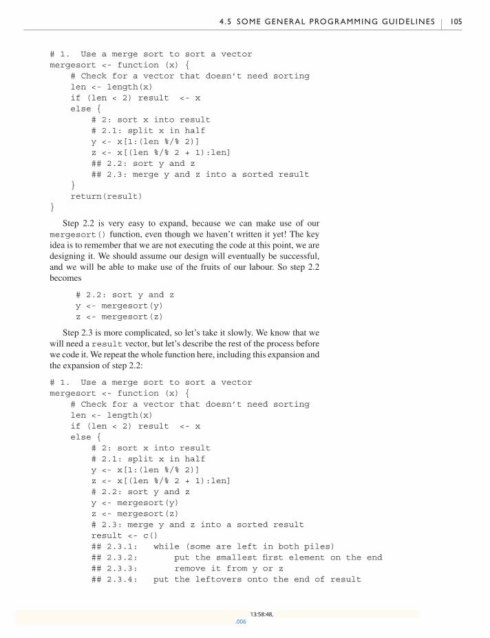
4 .5 SOME GENERAL PROGRAMMING GUIDELINES 105
# 1. Use a merge sort to sort a vectormergesort <- function (x) {
# Check for a vector that doesn’t need sortinglen <- length(x)if (len < 2) result <- xelse {
# 2: sort x into result# 2.1: split x in halfy <- x[1:(len %/% 2)]z <- x[(len %/% 2 + 1):len]## 2.2: sort y and z## 2.3: merge y and z into a sorted result
}return(result)
}
Step 2.2 is very easy to expand, because we can make use of ourmergesort() function, even though we haven’t written it yet! The keyidea is to remember that we are not executing the code at this point, we aredesigning it. We should assume our design will eventually be successful,and we will be able to make use of the fruits of our labour. So step 2.2becomes
# 2.2: sort y and zy <- mergesort(y)z <- mergesort(z)
Step 2.3 is more complicated, so let’s take it slowly. We know that wewill need a result vector, but let’s describe the rest of the process beforewe code it. We repeat the whole function here, including this expansion andthe expansion of step 2.2:
# 1. Use a merge sort to sort a vectormergesort <- function (x) {
# Check for a vector that doesn’t need sortinglen <- length(x)if (len < 2) result <- xelse {
# 2: sort x into result# 2.1: split x in halfy <- x[1:(len %/% 2)]z <- x[(len %/% 2 + 1):len]# 2.2: sort y and zy <- mergesort(y)z <- mergesort(z)# 2.3: merge y and z into a sorted resultresult <- c()## 2.3.1: while (some are left in both piles)## 2.3.2: put the smallest first element on the end## 2.3.3: remove it from y or z## 2.3.4: put the leftovers onto the end of result
.00613:58:48,
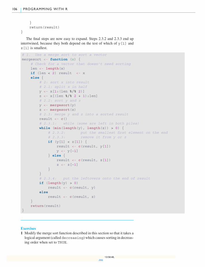
106 PROGRAMMING WITH R
}return(result)
}
The final steps are now easy to expand. Steps 2.3.2 and 2.3.3 end upintertwined, because they both depend on the test of which of y[1] andz[1] is smallest.
# 1. Use a merge sort to sort a vectormergesort <- function (x) {
# Check for a vector that doesn’t need sortinglen <- length(x)if (len < 2) result <- xelse {
# 2: sort x into result# 2.1: split x in halfy <- x[1:(len %/% 2)]z <- x[(len %/% 2 + 1):len]# 2.2: sort y and zy <- mergesort(y)z <- mergesort(z)# 2.3: merge y and z into a sorted resultresult <- c()# 2.3.1: while (some are left in both piles)while (min(length(y), length(z)) > 0) {
# 2.3.2: put the smallest first element on the end# 2.3.3: remove it from y or zif (y[1] < z[1]) {
result <- c(result, y[1])y <- y[-1]
} else {result <- c(result, z[1])z <- z[-1]
}}# 2.3.4: put the leftovers onto the end of resultif (length(y) > 0)
result <- c(result, y)else
result <- c(result, z)}return(result)
}
Exercises1 Modify the merge sort function described in this section so that it takes alogical argument (called decreasing) which causes sorting in decreas-ing order when set to TRUE.
.00613:58:48,

4 .6 DEBUGGING AND MAINTENANCE 107
2 The system of equations
f (x, y) = 0,
g(x, y) = 0
can be solved numerically using a form of Newton’s method. Assigninitial guesses to each of x0 and y0. Then perform the following iteration,for n = 1, 2, . . .:
xn = xn−1 − (gy,n−1 fn−1 − fy,n−1gn−1)/dn−1,
yn = yn−1 − ( fx,n−1gn−1 − gx,n−1 fn−1)/dn−1,
where
fx,n−1 = ∂ f
∂x(xn−1, yn−1),
fy,n−1 = ∂ f
∂y(xn−1, yn−1),
gx,n−1 = ∂g
∂x(xn−1, yn−1),
gy,n−1 = ∂g
∂y(xn−1, yn−1),
fn−1 = f (xn−1, yn−1),
gn−1 = g(xn−1, yn−1),
and
dn−1 = fx,n−1gy,n−1 − fy,n−1gx,n−1.
The iteration is terminated when the function values are close enoughto 0.(a) Write a function which will perform this iteration.(b) Apply the function to the system
x+ y = 0,
x2 + 2y2 − 2 = 0.
Find the two solutions to this system analytically as a check on yournumerical result.
4.6 Debugging and maintenance
Computer errors are called bugs. Removing these errors from a programis called debugging. Debugging is difficult, and one of our goals is towrite programs that don’t have bugs in them: but sometimes we makemistakes.
.00613:58:48,
108 PROGRAMMING WITH R
We have found that the following five steps help us to find and fix bugsin our own programs.
1. Recognize that a bug exists.2. Make the bug reproducible.3. Identify the cause of the bug.4. Fix the error and test.5. Look for similar errors.
We will consider each of these in turn.
4.6.1 Recognizing that a bug existsSometimes this is easy; if the program doesn’t work, there is a bug. How-ever, in other cases the program seems to work, but the output is incorrect,or the program works for some inputs, but not for others. A bug causingthis kind of error is much more difficult to recognize.
There are several strategies to make it easier. First, follow the advicein previous sections of this text, and break up your program into simple,self-contained functions. Document their inputs and outputs. Within thefunction, test that the inputs obey your assumptions about them, and thinkof test inputs where you can see at a glance whether the outputs match yourexpectations.
In some situations, it may be worthwhile writing two versions of a func-tion: one that may be too slow to use in practice, but which you are sure isright, and another that is faster but harder to be sure about. Test that bothversions produce the same output in all situations.
When errors occur only for certain inputs, our experience shows thatthose are often what are called edge cases: situations which are right on theboundary between legal and illegal inputs. Test those! For example, testwhat happens when you try a vector of length zero, test very large or verysmall values, etc.
4.6.2 Make the bug reproducibleBefore you can fix a bug, you need to know where things are going wrong.This is much easier if you know how to trigger the bug. Bugs that appearunpredictably are extremely difficult to fix. The good news is that for themost part computers are predictable: if you give them the same inputs, theygive you the same outputs. The difficulty is in working out what the neces-sary inputs are.
For example, a common mistake in programming is to misspell thename of a variable. Normally this results in an immediate error message,but sometimes you accidentally choose a variable that actually does exist.Then you’ll probably get the wrong answer, and the answer you get mayappear to be random, because it depends on the value in some unrelatedvariable.
The key to tracking down this sort of problem is to work hard to makethe error reproducible. Simplify things as much as possible: start a newempty R session, and see if you can reproduce it. Once you can reproducethe error, you will eventually be able to track it down.
.00613:58:48,
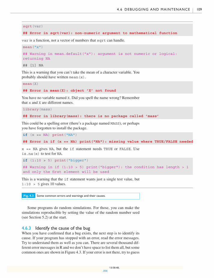
4 .6 DEBUGGING AND MAINTENANCE 109
sqrt(var)
## Error in sqrt(var): non-numeric argument to mathematical function
var is a function, not a vector of numbers that sqrt can handle.
mean("x")
## Warning in mean.default("x"): argument is not numeric or logical:returning NA
## [1] NA
This is a warning that you can’t take the mean of a character variable. Youprobably should have written mean(x).
mean(X)
## Error in mean(X): object ’X’ not found
You have no variable named X. Did you spell the name wrong? Rememberthat x and X are different names.
library(mass)
## Error in library(mass): there is no package called ’mass’
This could be a spelling error (there’s a package named MASS), or perhapsyou have forgotten to install the package.
if (x == NA) print("NA")
## Error in if (x == NA) print("NA"): missing value where TRUE/FALSE needed
x == NA gives NA, but the if statement needs TRUE or FALSE. Useis.na(x) to test for NA.
if (1:10 > 5) print("bigger")
## Warning in if (1:10 > 5) print("bigger"): the condition has length > 1and only the first element will be used
This is a warning that the if statement wants just a single test value, but1:10 > 5 gives 10 values.
Fig. 4.3 Some common errors and warnings and their causes.
Some programs do random simulations. For those, you can make thesimulations reproducible by setting the value of the random number seed(see Section 5.2) at the start.
4.6.3 Identify the cause of the bugWhen you have confirmed that a bug exists, the next step is to identify itscause. If your program has stopped with an error, read the error messages.Try to understand them as well as you can. There are several thousand dif-ferent error messages in R andwe don’t have space to list them all, but somecommon ones are shown in Figure 4.3. If your error is not there, try to guess
.00613:58:48,
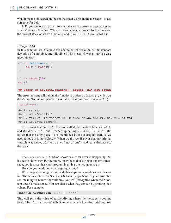
110 PROGRAMMING WITH R
what it means, or search online for the exact words in the message – or asksomeone for help.
In R, you can obtain extra information about an error message using thetraceback() function. When an error occurs, R saves information aboutthe current stack of active functions, and traceback() prints this list.
Example 4.18In this function we calculate the coefficient of variation as the standarddeviation of a variable, after dividing by its mean. However, our test casegives an error:
cv <- function(x) {sd(x / mean(x))
}
xl <- rnorm(10)cv(x1)
## Error in is.data.frame(x): object ’x1’ not found
The error message talks about the function is.data.frame(), which wedidn’t use. To find out where it was called from, we use traceback():
traceback()
## 4: cv(x1)## 3: sd(x/mean(x))## 2: var(if (is.vector(x)) x else as.double(x), na.rm = na.rm)## 1: is.data.frame(x)
This shows that our cv() function called the standard function sd(),and it called var(), and it ended up calling is.data.frame(). Butnotice that the only place x1 is mentioned is in our original call, so weneed to look at it more closely. When we do, we discover that our originalvariable was named xl (with an “ell,” not a “one”), and that’s the cause ofthe error.
The traceback() function shows where an error is happening, butit doesn’t show why. Furthermore, many bugs don’t trigger any error mes-sage, you just see that your program is giving the wrong answer.
How do you work out what is going wrong?With proper planning beforehand, this step can be made somewhat eas-
ier. The advice above in Section 4.6.1 also helps here. If you have cho-sen meaningful names for variables, you will recognize when their con-tent doesn’t make sense. You can check what they contain by printing theirvalues. For example,
cat("In myfunction, x=", x, "\n")
This will print the value of x, identifying where the message is comingfrom. The "\n" at the end tells R to go to a new line after printing. You
.00613:58:48,

4 .6 DEBUGGING AND MAINTENANCE 111
may want to use print() rather than cat() to take advantage of its for-matting, but remember that it can only print one thing at a time, so youwould likely use it as
cat("In myfunction, x=\n")print(x)
Amore flexible way to examine the values in functions is to use the RStudiodebugging facilities discussed in Section 4.6.6.
Another great way to understand what is going wrong in a small func-tion is to simulate it by hand. Act as you think R would act, and write downthe values of all variables as the function progresses. In combination withthe techniques described above, this can also identify misconceptions aboutR. If your simulation would print different results than the real R prints,then you’ve identified a possible cause of your bug: R is not behaving asyou expect. Most likely this is because you don’t know R well enough yet,but it is possible that you have actually discovered a bug in R!
4.6.4 Fixing errors and testingOnce you have identified the bug in your program, you need to fix it. Tryto fix it in such a way that you don’t cause a different problem. Then testwhat you’ve done! You should put together tests that include the way youknow that would reproduce the error, as well as edge cases, and anythingelse you can think of.
4.6.5 Look for similar errors elsewhereOften when you have found and fixed a bug, you can recognize the kindof mistake you made. It is worthwhile looking through the rest of yourprogram for similar errors, because if you made the mistake once, you mayhave made it twice.
4.6.6 Debugging in RStudioThe RStudio environment provides some very helpful support for under-standing the cause of errors when debugging. For example, if we hadentered Example 4.18 in the RStudio editor and executed it, we would havebeen offered the opportunity to produce a traceback in a single mouse click(Figure 4.4). While the ordering and numbering of the traceback entries isdifferent, the information is the same, and that might be enough to spot theerror. If not, you could look at the “Environment” pane at the top right ofthe display. It shows that xl really does exist.
If that’s still not enough of a hint as to what went wrong, you can seta breakpoint within the cv() function, and examine the state of variablesthere. Do this by clicking just to the left of the line number “4” in the codeeditor. A small red “stop sign” will appear. To activate the breakpoint, clickon “Source” in the top right of the code editor. This will run the whole fileagain, but with the breakpoint set, and execution will stop on line 4. TheEnvironment pane will show the values of local variables in the function.In this case it tells you that x has value x1 (Figure 4.5). You should noticethe typo at this point.
.00613:58:48,

112 PROGRAMMING WITH R
Fig. 4.4 Traceback ofExample 4.18 in RStudio.
Fig. 4.5 Breaking at line 4 ofExample 4.18 in RStudio.
In more complicated debugging situations, you might make use of thecontrols that now appear at the top of the Console pane. You can click onNext to execute one line of code, or use the other controls to “step into”a function, finish the current function, resume normal execution, or stopdebugging. Experiment!
4.6.7 The browser(), debug(), anddebugonce() functionsIf you are not using RStudio, the debugging facilities are still available,they are just a little less convenient. Instead of setting a breakpoint in the
.00613:58:48,
4 .7 EFF ICIENT PROGRAMMING 113
code editor, R allows you to call the function browser(). This will pauseexecution of your function, and allow you to examine (or change!) localvariables, or execute any other R command, inside the evaluation environ-ment of the function.
You can also execute a debugger command.
� n - “next”; execute the next line of code, single-stepping through thefunction
� s - “step into” function calls� f - “finish” the current function� c - “continue”; let the function continue running� Q - quit the debugger
Another way to enter the browser is to use the debug() function. Youmark function f for debugging using debug(f), and then the browserwill be called when you enter the function. Turn off debugging usingundebug(f). Alternatively, use debugonce() to mark the function, anddebugging will be turned off after the first call.
Exercises1 Consider the mergesort() function constructed in Example 4.17.
Using either the debug() function or the debugging facilities in RStu-dio, run mergesort(c(3, 5, 4, 2)) and check the value of the xargument before any other calculation is completed, and then the valuesof y and z just before sorting them.
2 Consider the cv() function constructed in Example 4.18. Using eitherthe debug() function or the debugging facilities in RStudio, runcv(c(-3, 10, -7)) and explain why it returns NaN. Suggest a morereasonable return value and modify the function to produce it.
4.7 Efficient programming
When producing computer code, you may find that it runs slower than youwant it to, even on today’s fast computers. But take heart: there are alwaysways to speed up a program. The process is called optimization. In thissection we will give a few examples of hand optimization in R: ways torewrite your code so that it runs faster. Other possibilities are automaticoptimization (not available in R, but some other programming platformscan do this), or hardware optimization, where you change your computerto run your programs faster, e.g. by buying a new one.
Optimization always requires some sort of trade-off. Hand optimiza-tion can be time consuming, and since optimized code can be harder tounderstand, errors can slip by undetected. You should always ensure thatyour code is correct before you try to optimize it because it will probably beharder to debug later. You should use judgment about whether optimizationwill be worthwhile.
.00613:58:48,
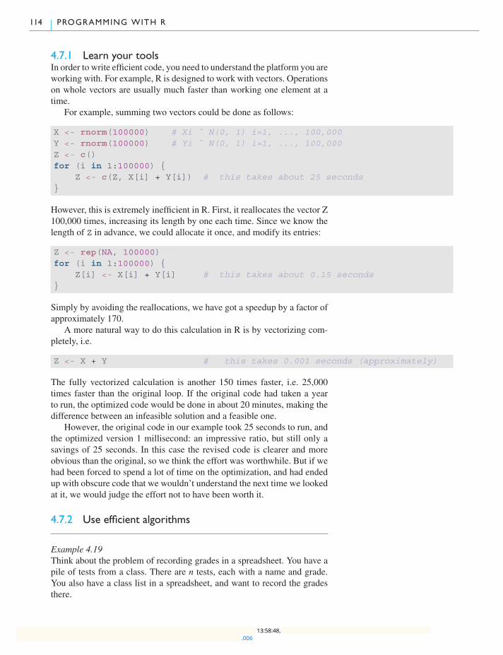
114 PROGRAMMING WITH R
4.7.1 Learn your toolsIn order to write efficient code, you need to understand the platform you areworking with. For example, R is designed to work with vectors. Operationson whole vectors are usually much faster than working one element at atime.
For example, summing two vectors could be done as follows:
X <- rnorm(100000) # Xi ˜ N(0, 1) i=1, ..., 100,000Y <- rnorm(100000) # Yi ˜ N(0, 1) i=1, ..., 100,000Z <- c()for (i in 1:100000) {
Z <- c(Z, X[i] + Y[i]) # this takes about 25 seconds}
However, this is extremely inefficient in R. First, it reallocates the vector Z100,000 times, increasing its length by one each time. Since we know thelength of Z in advance, we could allocate it once, and modify its entries:
Z <- rep(NA, 100000)for (i in 1:100000) {
Z[i] <- X[i] + Y[i] # this takes about 0.15 seconds}
Simply by avoiding the reallocations, we have got a speedup by a factor ofapproximately 170.
A more natural way to do this calculation in R is by vectorizing com-pletely, i.e.
Z <- X + Y # this takes 0.001 seconds (approximately)
The fully vectorized calculation is another 150 times faster, i.e. 25,000times faster than the original loop. If the original code had taken a yearto run, the optimized code would be done in about 20 minutes, making thedifference between an infeasible solution and a feasible one.
However, the original code in our example took 25 seconds to run, andthe optimized version 1 millisecond: an impressive ratio, but still only asavings of 25 seconds. In this case the revised code is clearer and moreobvious than the original, so we think the effort was worthwhile. But if wehad been forced to spend a lot of time on the optimization, and had endedup with obscure code that we wouldn’t understand the next time we lookedat it, we would judge the effort not to have been worth it.
4.7.2 Use efficient algorithms
Example 4.19Think about the problem of recording grades in a spreadsheet. You have apile of tests from a class. There are n tests, each with a name and grade.You also have a class list in a spreadsheet, and want to record the gradesthere.
.00613:58:48,

4 .7 EFF ICIENT PROGRAMMING 115
A really slow algorithm1. Read the name of the first student in the mark spreadsheet.2. Randomly select one of the n tests.3. If the names match, record the grade, and go on to the next student.4. If not, put the test back, and randomly select another.5. Continue until all grades have been recorded.
How bad is this algorithm? One answer to this question is to determinethe expected time until we get our first matching grade.
Since there are n tests, the probability of a correct match is 1/n. Thenumber of draws until the first match is a geometric random variable withparameter 1/n. The expected value for that random variable is known tobe n. When we get to the second student, the expected value will be n− 1,because there is one test fewer to search. Overall, the expected time to com-pletely record all of the grades is
∑ni=1 i = n(n− 1)/2 times the amount of
time to do one selection and check.
A slightly faster algorithm1. Take the first test.2. Scan through all the names in the spreadsheet until you find thematching
name, and record the grade.3. Repeat for each student.
For each test, this algorithm requires scanning an average of half thenames in the list, so the total time is n2/2 times the time to scan one name,plus n times the time to select a test from the pile. Even though this is a totalof n2/2 + n = n(n+ 2)/2 steps, each step is faster than the steps above, sothis algorithm is probably faster.
A much faster algorithm1. First, sort the names in the spreadsheet into alphabetical order.2. Take the first test.3. Search for the name in the spreadsheet, using the alphabetical sorting to
help.4. Repeat for each student.
This is much faster, because searching through a sorted list can bequicker, using a bisection technique: check the middle name, then the mid-dle name of whichever half the current test falls in, and so on. Each testtakes about log2 n comparisons before you’ll find it, so the whole operationtakes n log2 n operations. For a medium to large class this is much betterthan the n2/2 lookup time of the previous algorithm. For a class of 100, it’sthe difference between 5,000 operations and fewer than 700.
We could go further, and sort the tests before recording them: sincethe tests and the class list will be in the same order, the recording wouldtake just n steps. However, the sorting of the tests is probably much slowerthan sorting the names in the spreadsheet, since it requires physical sortingrather than just asking the computer to sort the names, and this will likelybe slower than the algorithm above. On the other hand, it leaves the tests insorted order so other future operations on them (e.g. looking up the test of
.00613:58:48,

116 PROGRAMMING WITH R
a particular student) would be faster. It will require a judgment regardingwhether the additional investment now will pay off in time saved later.
4.7.3 Measure the time your program takesOptimization is hard work, so you don’t want to do it when it’s not neces-sary. In many cases, it will take more time to optimize a program than youcould ever hope to save from the optimization. Before starting to optimize,you should measure the amount of time your program is taking, as an upperbound on the amount of time you could possibly save.
In R, the system.time() function measures the execution time ofevaluating expressions. For example,
X <- rnorm(100000)Y <- rnorm(100000)Z <- c()system.time({
for (i in 1:100000) {Z <- c(Z, X[i] + Y[i])
}})
## user system elapsed## 28.675 1.540 30.348
Z <- rep(NA, 100000)system.time({
for (i in 1:100000) {Z[i] <- X[i] + Y[i]
}})
## user system elapsed## 0.151 0.002 0.153
system.time(Z <- X + Y)
## user system elapsed## 0 0 0
shows how we obtained the timing reported above.6 The “user” time is the 6 The times here are not exactly thesame as before; this is typical, becauseother activities on the computer affectthe results.
time dedicated to this particular task, the “system” time is how much timeyour system spent doing other tasks, and the “elapsed” time is the time wewould have seen on a clock. The microbenchmark package automati-cally repeats operations a number of times to allow measurement of veryshort durations, e.g.
library(microbenchmark)microbenchmark(Z <- X + Y)
## Unit: microseconds## expr min lq mean median uq max neval## Z <- X + Y 98.627 115.762 310.9959 148.1575 178.802 3099.206 100
.00613:58:48,

CHAPTER EXERCISES 117
Youmay also be able to measure which particular parts of your programare the best targets for optimization. A famous rule of thumb in computingis the 90/10 rule: 90% of the execution time of your program comes from10% of the code. We call code in the slow 10% the bottlenecks. The corol-lary is that if you can identify and optimize the bottlenecks, you can obtaina substantial speedup without even looking at 90% of the program.
Many software platforms offer profilers to help find the bottlenecks inyour program. There are various kinds of profilers, but in general they mon-itor the program while it is running and report on where the execution timewas spent. In R the profiler is controlled by the Rprof() function, but adiscussion of the details is beyond the scope of this text.
4.7.4 Be willing to use different toolsMuch as we love it, we admit that R is not the only computing platformavailable, and it is not the best tool for all tasks. For raw speed, you aremuch better off using a compiled language like C, C++, or Fortran. R itselfis written in C and Fortran, which is why the operations on vectors go soquickly: most of the work is done in compiled code.
A style of programming that we recommend is to do most of yourwork in R. In cases where you don’t get acceptable speed, identify thebottlenecks, and consider translating those into a compiled language. Rhas extensive support for linking to code in other languages. Unfortunatelythis requires a level of technical detail that is again beyond the scope of thisbook.
4.7.5 Optimize with careThe famous computer scientist Donald Knuth once said that “Prematureoptimization is the root of all evil (or at least most of it) in programming.”We have emphasized above that optimization is difficult and that it is notalways advisable.We finish the chapter with this advice for writing efficientcode.
1. Get it right.2. Get it fast enough.3. Make sure it’s still right.
Chapter exercises1 As mentioned in Example 4.2, the RANDU algorithm produces tripletsof values that are very predictable. To see this, try the following. First,generate 3,000,000 values using RANDU. Round the values to threedecimal places, and put them into a matrix with three columns, withthe first value in column 1, the second in column 2, and the third incolumn 3, repeated through the whole vector of values. Then set x to0.1 and find the subset of rows of the matrix where the first columnequals x. Plot the second column versus the third column. Repeat thisfor x = 0.1, 0.2, . . . , 0.9 in an array of nine plots. The pattern should bestriking.
.00613:58:48,

118 PROGRAMMING WITH R
2 Write a function which will evaluate polynomials of the form
P(x) = cnxn−1 + cn−1x
n−2 + · · · + c2x+ c1.
Your function should take x and the vector of polynomial coefficientsas arguments and it should return the value of the evaluated polynomial.Call this function directpoly().
3 Refer to the previous question. For moderate to large values of n, evalu-ation of a polynomial at x can be done more efficiently using Horner’srule.(a) Set an ← cn.(b) For i = n− 1, . . . , 1, set ai = ai+1x+ ci.(c) Return a1. (This is the computed value of P(x).)Write an R function which takes arguments x and a vector of polynomialcoefficients and which returns the value of the polynomial evaluated at x.Call the resulting function hornerpoly(). Ensure that your functionreturns an appropriate vector of values when x is a vector.
4 Do some timings to compare the algorithms used in the previous twoexercises.(a) In particular, try the following code:
system.time(directpoly(x = seq(-10, 10, length = 5000000),c(1, -2, 2, 3, 4, 6, 7)))
system.time(horner(x = seq(-10, 10, length = 5000000),c(1, -2, 2, 3, 4, 6, 7)))
(b) What happens to the comparison when the number of polynomialcoefficients is smaller? Try
P(x) = 2x2 + 17x− 3.
5 Using a starting value of 2.9, find the time required for Newton’s methodto find the zero (to within 7-digit accuracy) of(a) (x− 3)e−x
(b) (x2 − 6x+ 9)e−x
6 Repeat the previous question, using the bisection algorithm and the ini-tial interval [2.1, 3.1].
7 Do a timing comparison of the bubble sort (see Example 4.16) and themerge sort (see Example 4.17). Do the comparison for vectors of length10, 1000, 10000, and 100000. (You may use the function rnorm() togenerate vectors for this purpose.)
8 This exercise gives a taste of the graphical editing capability of grid(touched on briefly in Chapter 3). To create a graphical object (grob)with the information required to draw a triangle, execute the following:
b1 <- sqrt(1/cos(36*pi/180)ˆ2-1)/2b2 <- sin(72*pi/180)/(2*(1+cos(72*pi/180))) - (1-sin(72*pi/180))/2triangle <- polygonGrob(c(0,.5,1), c(b2,b2+b1,b2),
name = "triangle", gp = gpar(fill = "yellow", col = 0))grid.draw(triangle) # nothing appears until this line is executed
.00613:58:48,

CHAPTER EXERCISES 119
Next draw three rotated copies of the triangles, creating the impressionof a star shape:
for (i in 0:2){pushViewport(vp=viewport(angle=72*i))grid.draw(triangle)upViewport()}
.00613:58:48,
5
Simulation
Much of statistics relies on being able to evaluate expectations of randomvariables, and finding quantiles of distributions.1 Here are some examples. 1 See the appendix if you need a review
of random variables and their properties.� In hypothesis testing, the p-value of a sample is defined as the probabilityof observing data at least as extreme as the sample in hand, given that thenull hypothesis is true. This is the expected value of a random variabledefined to be 0 when a sample is less extreme, and 1 otherwise.
� The bias of an estimator is defined to be the expected value of the esti-mator minus the true value that it is estimating.
� Confidence intervals are based on quantiles of the distribution of a pivotalquantity, e.g. (X − μ)/(s/
√n).
In simple cases we may evaluate these quantities analytically, or use largesample approximations. However, in other cases we need computer-basedmethods to approximate them.
In this chapter, you will be introduced to Monte Carlo simulation. Thisintroduction will include basic ideas of random (or, more properly, pseu-dorandom) number generation. You will then see how to simulate randomvariables from several of the common probability distributions. Next, wewill show you how simulation can be used in some surprising ways: tomodel natural processes and to evaluate integrals. The final topics of thechapter on Markov chains, as well as rejection and importance samplingwill give you a hint as to what more advanced methods are like.
5.1 Monte Carlo simulation
One of the most general computer-based methods for approximating prop-erties of random variables is the Monte Carlo method.
To approximate the mean μ = E(X ) using the Monte Carlo method,we generate m independent and identically distributed (i.i.d.) copies of X ,namely X1, . . . ,Xm, and use the sample mean X = (1/m)
∑Xi as an esti-
mate of E(X ). For large values of m, X gives a good approximation toE(X ).2 2 This follows from the law of large
numbers.Furthermore, ifm is large the distribution of the sample mean, X , can beapproximated3 by a normal distribution with mean μ and variance σ 2/m. 3 This is the central limit theorem.
.00714:02:22,
5 .2 GENERATION OF PSEUDORANDOM NUMBERS 121
Here σ 2 is the variance Var(X ), which can be approximated by the sam-ple variance s2 = [1/(m− 1)]
∑(Xi − X )2. This allows us to construct
approximate confidence intervals for μ. For example, X ± 1.96s/√m will
contain μ approximately 95% of the time.The remainder of this chapter describes methods for simulating the gen-
eration of random variables on a computer. We will describe deterministicmethods of generating values, which are then treated as though they arerandom. It is useful to think of two participants in this process: the program-mer hiding behind a curtain knows that the algorithms are deterministic andpredictable, but the user of those numbers is unaware of the mechanismsused to compute them, so, to that user, the numbers appear random andunpredictable. In practice, both participants may be the same person! Todistinguish this scheme from true random numbers which really are unpre-dictable, we will call our simulated random numbers pseudorandom num-bers in the remainder of the chapter.
5.2 Generation of pseudorandom numbers
We begin our discussion of simulation with a brief exploration of themechanics of pseudorandom number generation. In particular, we willdescribe one of the simplest methods for simulating independent uniformrandom variables on the interval [0,1].
A multiplicative congruential random number generator produces asequence of pseudorandom numbers, u0, u1, u2, . . . , which appear similarto independent uniform random variables on the interval [0,1].
Let m be a large integer, and let b be another integer which is smallerthan m. The value of b is often chosen to be near the square root of m.Different values of b and m give rise to pseudorandom number generatorsof varying quality. There are various criteria available for choosing goodvalues of these parameters, but it is always important to test the resultinggenerator to ensure that it is providing reasonable results.
To begin, an integer x0 is chosen between 1 and m. x0 is called the seed.We discuss strategies for choosing x0 below.
Once the seed has been chosen, the generator proceeds as follows:
x1 = bx0 (mod m),
u1 = x1/m.
u1 is the first pseudorandom number, taking some value between 0 and 1.The second pseudorandom number is then obtained in the same manner:
x2 = bx1 (mod m),
u2 = x2/m.
u2 is another pseudorandom number. Ifm and b are chosen properly and arenot disclosed to the user, it is difficult to predict the value of u2, given thevalue of u1 only. In other words, for most practical purposes u2 is approxi-mately independent of u1. Themethod continues according to the following
.00714:02:22,

122 S IMULATION
formulas:
xn = bxn−1 (mod m),
un = xn/m.
This method produces numbers which are entirely deterministic, but toan observer who doesn’t know the formula above, the numbers appear tobe random and unpredictable, at least in the short term.
Example 5.1Take m = 7 and b = 3. Also, take x0 = 2. Then
x1 = 3 × 2 (mod 7) = 6, u1 = 0.857,x2 = 3 × 6 (mod 7) = 4, u2 = 0.571,x3 = 3 × 4 (mod 7) = 5, u3 = 0.714,x4 = 3 × 5 (mod 7) = 1, u4 = 0.143,x5 = 3 × 1 (mod 7) = 3, u5 = 0.429,x6 = 3 × 3 (mod 7) = 2, u6 = 0.286.
It should be clear that the iteration will set x7 = x1 and cycle xi through thesame sequence of integers, so the corresponding sequence ui will also becyclic. An observer might not easily be able to predict u2 from u1, but sinceui+6 = ui for all i > 0, longer sequences are very easy to predict. In orderto produce an unpredictable sequence, it is desirable to have a very largecycle length so that it is unlikely that any observer will ever see a wholecycle. The cycle length cannot be any larger than m, so m would normallybe taken to be very large.
Care must be taken in the choice of b and m to ensure that the cyclelength is actually m. Note, for example, what happens when b = 171 andm = 29241. Start with x0 = 3, say:
x1 = 171 × 3 = 513,
x2 = 171 × 513 (mod 29241) = 0.
All remaining xn values will be 0. To avoid this kind of problem, we shouldchoosem so that it is not divisible by b; thus, prime values ofmwill be pre-ferred. The next example gives a generator with somewhat better behavior.
Example 5.2The following lines produce 50 pseudorandom numbers based on the mul-tiplicative congruential generator
xn = 171xn−1 (mod 30269),
un = xn/30269,
with initial seed x0 = 27218:
.00714:02:22,

5 .2 GENERATION OF PSEUDORANDOM NUMBERS 123
random.number <- numeric(50) # this will store the# pseudorandom output
random.seed <- 27218for (j in 1:50) {
random.seed <- (171 * random.seed) %% 30269random.number[j] <- random.seed / 30269
}
The results, stored in the vector random.number, are as follows. Notethat the vector elements range between 0 and 1. These are the pseudoran-dom numbers, u1, u2, . . . , u50.
random.number
## [1] 0.76385080 0.61848756 0.76137302 0.19478675 0.30853348 0.75922561## [7] 0.82757937 0.51607255 0.24840596 0.47741914 0.63867323 0.21312234## [13] 0.44391952 0.91023820 0.65073177 0.27513297 0.04773861 0.16330239## [19] 0.92470845 0.12514454 0.39971588 0.35141564 0.09207440 0.74472232## [25] 0.34751726 0.42545178 0.75225478 0.63556774 0.68208398 0.63636063## [31] 0.81766824 0.82126929 0.43704780 0.73517460 0.71485678 0.24051009## [37] 0.12722587 0.75562457 0.21180085 0.21794575 0.26872378 0.95176583## [43] 0.75195745 0.58472364 0.98774324 0.90409330 0.59995375 0.59209092## [49] 0.24754700 0.33053619
A similar kind of operation (though using a different formula, and witha much longer cycle) is used internally by R to produce pseudorandomnumbers automatically with the function runif().
Syntaxrunif(n, min = a, max = b)
Execution of this command produces n pseudorandom uniform num-bers on the interval [a, b]. The default values are a = 0 and b = 1. Theseed is selected internally.
Example 5.3Generate 5 uniform pseudorandom numbers on the interval [0, 1], and 10uniform such numbers on the interval [−3,−1].
runif(5)
## [1] 0.9502223 0.3357378 0.1330718 0.4901114 0.0607455
runif(10, min = -3, max = -1)
## [1] -2.284105 -2.545768 -2.199852 -1.126908 -1.324746 -2.744848## [7] -1.549739 -1.445740 -2.834744 -1.372574
If you execute the above code yourself, you will almost certainly obtaindifferent results than those displayed in our output. This is because the
.00714:02:22,
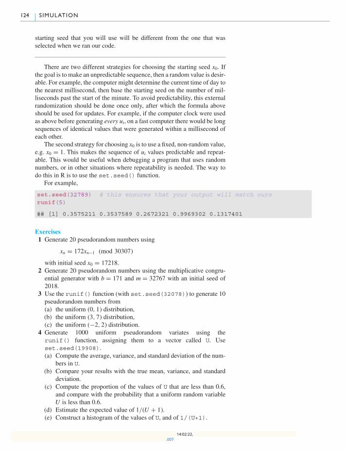
124 S IMULATION
starting seed that you will use will be different from the one that wasselected when we ran our code.
There are two different strategies for choosing the starting seed x0. Ifthe goal is to make an unpredictable sequence, then a random value is desir-able. For example, the computer might determine the current time of day tothe nearest millisecond, then base the starting seed on the number of mil-liseconds past the start of the minute. To avoid predictability, this externalrandomization should be done once only, after which the formula aboveshould be used for updates. For example, if the computer clock were usedas above before generating every ui, on a fast computer there would be longsequences of identical values that were generated within a millisecond ofeach other.
The second strategy for choosing x0 is to use a fixed, non-random value,e.g. x0 = 1. This makes the sequence of ui values predictable and repeat-able. This would be useful when debugging a program that uses randomnumbers, or in other situations where repeatability is needed. The way todo this in R is to use the set.seed() function.
For example,
set.seed(32789) # this ensures that your output will match oursrunif(5)
## [1] 0.3575211 0.3537589 0.2672321 0.9969302 0.1317401
Exercises1 Generate 20 pseudorandom numbers using
xn = 172xn−1 (mod 30307)
with initial seed x0 = 17218.2 Generate 20 pseudorandom numbers using the multiplicative congru-ential generator with b = 171 and m = 32767 with an initial seed of2018.
3 Use the runif() function (with set.seed(32078)) to generate 10pseudorandom numbers from(a) the uniform (0, 1) distribution,(b) the uniform (3, 7) distribution,(c) the uniform (−2, 2) distribution.
4 Generate 1000 uniform pseudorandom variates using therunif() function, assigning them to a vector called U. Useset.seed(19908).(a) Compute the average, variance, and standard deviation of the num-
bers in U.(b) Compare your results with the true mean, variance, and standard
deviation.(c) Compute the proportion of the values of U that are less than 0.6,
and compare with the probability that a uniform random variableU is less than 0.6.
(d) Estimate the expected value of 1/(U + 1).(e) Construct a histogram of the values of U, and of 1/(U+1).
.00714:02:22,

5 .2 GENERATION OF PSEUDORANDOM NUMBERS 125
5 Simulate 10000 independent observations on a uniformly distributedrandom variable on the interval [3.7, 5.8].(a) Estimate the mean, variance, and standard deviation of such a uni-
form random variable and compare your estimates with the truevalues.
(b) Estimate the probability that such a random variable is greater than4.0. Compare with the true value.
6 Simulate 10000 values of a uniform (0, 1) random variable, U1, usingrunif(), and simulate another set of 10000 values of a uniform (0, 1)random variable U2. Assign these vectors to U1 and U2, respectively.Since the values in U1 and U2 are approximately independent, we canviewU1 andU2 as independent uniform (0, 1) random variables.(a) Estimate E[U1 +U2]. Compare with the true value, and compare
with an estimate of E[U1] + E[U2].(b) Estimate Var(U1 +U2) and Var(U1) + Var(U2). Are they equal?
Should the true values be equal?(c) Estimate P(U1 +U2 ≤ 1.5).(d) Estimate P(
√U1 + √
U2) ≤ 1.5).7 SupposeU1,U2, andU3 are independent uniform random variables onthe interval (0, 1). Use simulation to estimate the following quantities.(a) E[U1 +U2 +U3].(b) Var(U1 +U2 +U3) and Var(U1) + Var(U2) + Var(U3).(c) E[
√U1 +U2 +U3].
(d) P(√U1 + √
U2 + √U3 ≥ 0.8).
8 Use the round() function together with runif() to generate 1000pseudorandom integers which take values from 1 through 10, assign-ing these values to a vector called discreteunif. Use the table()function to check whether the observed frequencies for each value areclose to what you expect. If they are not close, how should you modifyyour procedure?
9 The sample() function allows you to take a simplerandom sample from a vector of values. For example,sample(c(3,5,7), size = 2, replace = FALSE) willyield a vector of two values taken (without replacement) from the set{3, 5, 7}. Use the sample() function to generate 50 pseudorandomintegers from 1 through 100,(a) sampled without replacement,(b) sampled with replacement.
10 The following code simulates the sum (X) and difference (Y ) of twouniform random variables (U1 and U2). A scatterplot of Y versus X isthen displayed and the correlation between X and Y is estimated.
U2 <- runif(1000)U1 <- runif(1000)X <- U1 + U2Y <- U1 - U2plot(Y ˜ X)cor(X,Y) # this calculates the sample correlation
The correlation gives a measure of linear dependence between two ran-dom variables. A value near 0 indicates that there is almost no such
.00714:02:22,
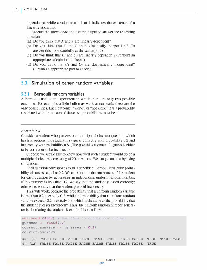
126 S IMULATION
dependence, while a value near −1 or 1 indicates the existence of alinear relationship.
Execute the above code and use the output to answer the followingquestions.(a) Do you think that X and Y are linearly dependent?(b) Do you think that X and Y are stochastically independent? (To
answer this, look carefully at the scatterplot.)(c) Do you think that U1 and U2 are linearly dependent? (Perform an
appropriate calculation to check.)(d) Do you think that U1 and U2 are stochastically independent?
(Obtain an appropriate plot to check.)
5.3 Simulation of other random variables
5.3.1 Bernoulli random variablesA Bernoulli trial is an experiment in which there are only two possibleoutcomes. For example, a light bulb may work or not work; these are theonly possibilities. Each outcome (“work”, or “not work”) has a probabilityassociated with it; the sum of these two probabilities must be 1.
Example 5.4Consider a student who guesses on a multiple choice test question whichhas five options; the student may guess correctly with probability 0.2 andincorrectly with probability 0.8. (The possible outcome of a guess is eitherto be correct or to be incorrect.)
Suppose we would like to know how well such a student would do on amultiple choice test consisting of 20 questions. We can get an idea by usingsimulation.
Each question corresponds to an independent Bernoulli trial with proba-bility of success equal to 0.2.We can simulate the correctness of the studentfor each question by generating an independent uniform random number.If this number is less than 0.2, we say that the student guessed correctly;otherwise, we say that the student guessed incorrectly.
This will work, because the probability that a uniform random variableis less than 0.2 is exactly 0.2, while the probability that a uniform randomvariable exceeds 0.2 is exactly 0.8, which is the same as the probability thatthe student guesses incorrectly. Thus, the uniform random number genera-tor is simulating the student. R can do this as follows:
set.seed(23207) # use this to obtain our outputguesses <- runif(20)correct.answers <- (guesses < 0.2)correct.answers
## [1] FALSE FALSE FALSE FALSE TRUE TRUE TRUE FALSE TRUE TRUE FALSE## [12] FALSE FALSE FALSE FALSE FALSE FALSE FALSE FALSE TRUE
.00714:02:22,
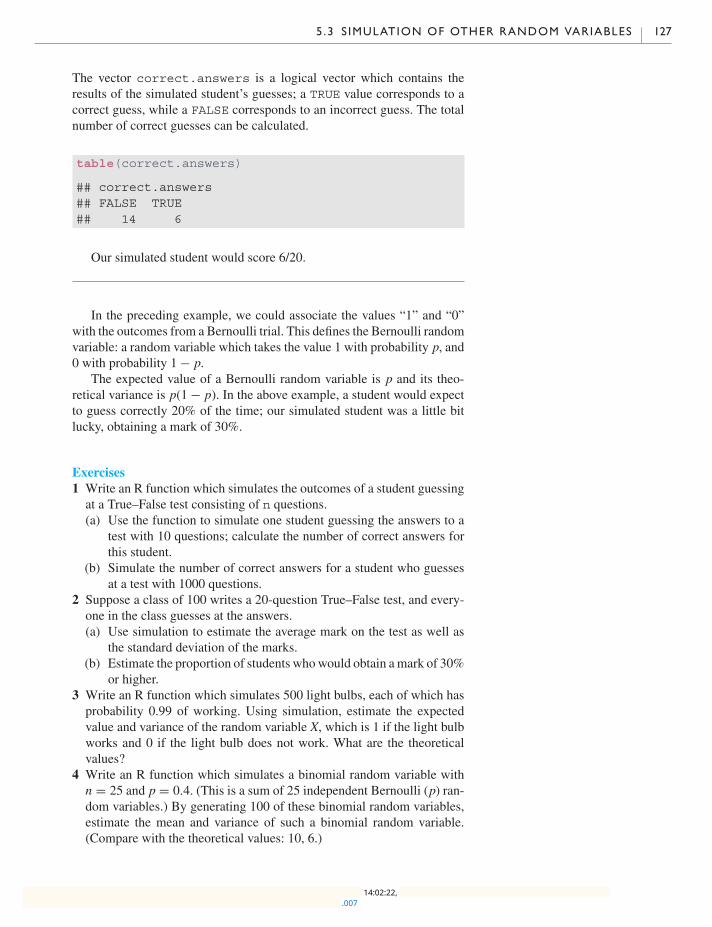
5 .3 S IMULATION OF OTHER RANDOM VARIABLES 127
The vector correct.answers is a logical vector which contains theresults of the simulated student’s guesses; a TRUE value corresponds to acorrect guess, while a FALSE corresponds to an incorrect guess. The totalnumber of correct guesses can be calculated.
table(correct.answers)
## correct.answers## FALSE TRUE## 14 6
Our simulated student would score 6/20.
In the preceding example, we could associate the values “1” and “0”with the outcomes from a Bernoulli trial. This defines the Bernoulli randomvariable: a random variable which takes the value 1 with probability p, and0 with probability 1 − p.
The expected value of a Bernoulli random variable is p and its theo-retical variance is p(1 − p). In the above example, a student would expectto guess correctly 20% of the time; our simulated student was a little bitlucky, obtaining a mark of 30%.
Exercises1 Write an R function which simulates the outcomes of a student guessingat a True–False test consisting of n questions.(a) Use the function to simulate one student guessing the answers to a
test with 10 questions; calculate the number of correct answers forthis student.
(b) Simulate the number of correct answers for a student who guessesat a test with 1000 questions.
2 Suppose a class of 100 writes a 20-question True–False test, and every-one in the class guesses at the answers.(a) Use simulation to estimate the average mark on the test as well as
the standard deviation of the marks.(b) Estimate the proportion of students whowould obtain amark of 30%
or higher.3 Write an R function which simulates 500 light bulbs, each of which hasprobability 0.99 of working. Using simulation, estimate the expectedvalue and variance of the random variable X, which is 1 if the light bulbworks and 0 if the light bulb does not work. What are the theoreticalvalues?
4 Write an R function which simulates a binomial random variable withn = 25 and p = 0.4. (This is a sum of 25 independent Bernoulli (p) ran-dom variables.) By generating 100 of these binomial random variables,estimate the mean and variance of such a binomial random variable.(Compare with the theoretical values: 10, 6.)
.00714:02:22,
128 S IMULATION
5.3.2 Binomial random variablesLet X denote the sum of m independent Bernoulli random variables, eachhaving probability p. X is called a binomial random variable; it representsthe number of “successes” in m Bernoulli trials.
A binomial random variable can take values in the set {0, 1, 2, . . . ,m}.The probability of a binomial random variable X taking on any one of thesevalues is governed by the binomial distribution:
P(X = x) =(m
x
)px(1 − p)m−x, x = 0, 1, 2, . . . ,m.
These probabilities can be computed using the dbinom() function.
Syntaxdbinom(x, size, prob)
Here, size and prob are the binomial parameters m and p, respectively,while x denotes the number of “successes.” The output from this functionis the value of P(X = x).
Example 5.5Compute the probability of getting four heads in six tosses of a fair coin.
dbinom(x = 4, size = 6, prob = 0.5)
## [1] 0.234375
Thus, P(X = 4) = 0.234, when X is a binomial random variable withm = 6 and p = 0.5.
Cumulative probabilities of the form P(X ≤ x) can be computed usingpbinom(); this function takes the same arguments as dbinom(). Forexample, we can calculate P(X ≤ 4), where X is the number of headsobtained in six tosses of a fair coin, as
pbinom(4, 6, 0.5)
## [1] 0.890625
The function qbinom() gives the quantiles for the binomial distribu-tion. The 89th percentile of the distribution of X (as defined above) is
qbinom(0.89, 6, 0.5)
## [1] 4
The expected value (or mean) of a binomial random variable is mp andthe variance is mp(1 − p).
The rbinom() function can be used to generate binomial pseudoran-dom numbers.
.00714:02:22,
5 .3 S IMULATION OF OTHER RANDOM VARIABLES 129
Syntaxrbinom(n, size, prob)
Here, size and prob are the binomial parameters, while n is the numberof variates generated.
Example 5.6Suppose 10% of the water heater dip tubes produced by a machine aredefective, and suppose 15 tubes are produced each hour. Each tube is inde-pendent of all other tubes. This process is judged to be out of control whenmore than four defective tubes are produced in any single hour. Simulatethe number of defective tubes produced by the machine for each hour overa 24-hour period, and determine whether any process should have beenjudged out of control at any point in that simulation run.
Since 15 tubes are produced each hour and each tube has a 0.1 prob-ability of being defective, which is independent of the state of the othertubes, the number of defectives produced in one hour is a binomial randomvariable with m = 15 and p = 0.1. To simulate the number of defectivesfor each hour in a 24-hour period, we need to generate 24 binomial randomnumbers. We then identify all instances in which the number of defectivesexceeds 5. One such simulation run is
defectives <- rbinom(24, 15, 0.1)defectives
## [1] 0 1 1 0 1 1 2 5 0 0 1 1 3 3 0 2 2 0 1 0 1 1 4 2
any(defectives > 5)
## [1] FALSE
Exercises1 Suppose the proportion defective is 0.15 for a manufacturing operation.Simulate the number of defectives for each hour of a 24-hour period,assuming 25 units are produced each hour. Check whether the number ofdefectives ever exceeds 5. Repeat, assuming p = 0.2 and then p = 0.25.
2 Simulate 10000 binomial pseudorandom numbers with parameters 20and 0.3, assigning them to a vector called binsim. Let X be a Bino-mial(20, 0.3) random variable. Use the simulated numbers to estimatethe following.(a) P(X ≤ 5).(b) P(X = 5).(c) E[X].(d) Var(X ).(e) The 95th percentile of X . (You may use the quantile() function.)(f) The 99th percentile of X .(g) The 99.9999th quantile of X .In each case, compare your estimates with the true values. What isrequired to estimate extreme quantities accurately?
.00714:02:22,
130 S IMULATION
3 Use simulation to estimate the mean and variance of a binomial ran-dom variable with n = 18 and p = 0.76. Compare with the theoreticalvalues.
4 Consider the following function which is designed to simulate binomialpseudorandom variates using the so-called inversion method.
ranbin <- function(n, size, prob) {cumpois <- pbinom(0:(size - 1), size, prob)singlenumber <- function() {
x <- runif(1)N <- sum(x > cumpois)N
}replicate(n, singlenumber())
}
(a) Study this function carefully and write documentation for it.4 Note, 4 The replicate() functionallows us to repeatedly callsinglenumber(), assigning n resultsto a vector. See help(replicate) formore information.
particularly, what the operations in the singlenumber() functionare for.
(b) Use ranbin() to simulate vectors of length 1000, 10000, and100000 from the binomial distribution with size parameter 10 andprobability parameter 0.4. Use the system.time() function tocompare the execution times for these simulations with the corre-sponding execution times when rbinom() is used.
5 The following function simulates binomial pseudorandom numbersby summing up the corresponding independent Bernoulli randomvariables.
ranbin2 <- function(n, size, prob) {singlenumber <- function(size, prob) {
x <- runif(size)N <- sum(x < prob)N
}replicate(n, singlenumber(size, prob))
}
(a) Study this function carefully and write documentation for it. Note,particularly, what the operations in the singlenumber() functionare for.
(b) Use ranbin2() to simulate vectors of length 10000 from thebinomial distribution with size parameters 10, 100, and 1000, andprobability parameter 0.4. Use the system.time() function tocompare the execution times for these simulations with the corre-sponding execution times when rbinom() is used. Compare withexecution times from the ranbin() function created in the previ-ous exercise.
6 The generator in the previous exercise required size uniform pseudo-random numbers to be generated for each binomial number generated.The following generator is based on the same principle as the previous
.00714:02:22,
5 .3 S IMULATION OF OTHER RANDOM VARIABLES 131
one, but requires only one uniform pseudorandom number to be gener-ated for each binomial number generated.
ranbin3 <- function(n, size, prob) {singlenumber <- function(size, prob) {
k <- 0U <- runif(1)X <- numeric(size)while (k < size) {
k <- k + 1if (U <= prob) {
X[k] <- 1U <- U / prob
} else {X[k] <- 0U <- (U - prob)/(1 - prob)
}}return(sum(X))
}replicate(n, singlenumber(size, prob))
}
(a) Use the ranbin3() function to generate 100 pseudorandom num-bers from binomial distributions with parameters(i) size = 20 and prob = 0.4,(ii) size = 500 and prob = 0.7.
(b) What is the conditional distribution ofU/p, given thatU < p?(c) What is the conditional distribution of (U − p)/(1 − p), given that
U > p?(d) Use the answers to the above questions to provide documentation
for the ranbin3() function.7 One version of the central limit theorem says that if X is a binomialrandom variable with parameters m and p, and
Z = X − mp√mp(1 − p)
,
then Z is approximately standard normal, and the approximationimproves as m gets large.
The following code simulates a large number of such Z values forvalues of m in the set {1, 2, . . . , 100} and plots a normal QQ plot in eachcase.
for (m in 1:100) {z <- (rbinom(20000, size = m, prob = 0.4) - m * 0.4) /
sqrt(m * 0.4 * 0.6)qqnorm(z, ylim = c(-4, 4), main = paste("QQ-plot, m = ", m))qqline(z)
}
(a) Execute the code and observe how the distribution of Z changes asm increases.
.00714:02:22,
132 S IMULATION
(b) Modify the code so that a similar “movie” is produced for the caseswhere p = 0.3, 0.2, 0.1, and 0.05, respectively. How largemustm bebefore you see a reasonably straight line in the QQ plot? Ism = 100satisfactorily large in all cases?
5.3.3 Poisson random variablesThe Poisson distribution is the limit of a sequence of binomial distribu-tions with parameters n and pn, where n is increasing to infinity, and pnis decreasing to 0, but where the expected value (or mean) npn convergesto a constant λ. The variance npn(1 − pn) converges to this same constant.Thus, the mean and variance of a Poisson random variable are both equalto λ. This parameter is sometimes referred to as a rate.
Poisson random variables arise in a number of different ways. They areoften used as a crude model for count data. Examples of count data arethe numbers of earthquakes in a region in a given year, or the number ofindividuals who arrive at a bank teller in a given hour. The limit comes fromdividing the time period into n independent intervals, on which the countis either 0 or 1. The Poisson random variable is the total count.
The possible values that a Poisson random variable X could take arethe non-negative integers {0, 1, 2, . . .}. The probability of taking on any ofthese values is
P(X = x) = e−xλx
x!, x = 0, 1, 2, . . . .
These probabilities can be evaluated using the dpois() function.
Syntaxdpois(x, lambda)
Here, lambda is the Poisson rate parameter, while x is the number of Pois-son events. The output from the function is the value of P(X = x).
Example 5.7According to the Poisson model, the probability of three arrivals at an auto-matic bank teller in the next minute, where the average number of arrivalsper minute is 0.5, is
dpois(x = 3, lambda = 0.5)
## [1] 0.01263606
Therefore, P(X = 3) = 0.0126, if X is a Poisson random variable withmean 0.5.
Cumulative probabilities of the form P(X ≤ x) can be calculated usingppois(), and Poisson quantiles can be computed using qpois().
We can generate Poisson randomnumbers using therpois() function.
.00714:02:22,
5 .3 S IMULATION OF OTHER RANDOM VARIABLES 133
Syntaxrpois(n, lambda)
The parameter n is the number of variates produced, and lambda is asabove.
Example 5.8Suppose traffic accidents occur at an intersection with a mean rate of 3.7per year. Simulate the annual number of accidents for a 10-year period,assuming a Poisson model.
rpois(10, 3.7)
## [1] 6 7 2 3 5 7 6 2 4 4
Poisson processesA Poisson process is a simple model of the collection of events that occurduring an interval of time. A way of thinking about a Poisson process is tothink of a random collection of points on a line or in the plane (or in higherdimensions, if necessary).
The homogeneous Poisson process has the following properties.
1. The distribution of the number of points in a set is Poisson with rateproportional to the size of the set.
2. The numbers of points in non-overlapping sets are independent of eachother.
In particular, for a Poisson process with rate λ the number of points on aninterval [0,T ] is Poisson distributed with mean λT . One way to simulatethis is as follows.
1. Generate N as a Poisson pseudorandom number with parameter λT .2. Generate N independent uniform pseudorandom numbers on the inter-
val [0,T ].
Example 5.9Simulate points of a homogeneous Poisson process having rate 1.5 on theinterval [0, 10].
N <- rpois(1, 1.5 * 10)P <- runif(N, max = 10)sort(P)
## [1] 0.0321442 0.1173187 0.2542297 2.4376206 3.9358325 4.0503778## [7] 4.5093112 5.2883388 7.4392293 8.4700712 8.7615109 8.8157830## [13] 9.3580064
.00714:02:22,
134 S IMULATION
Exercises1 Simulate the number of accidents for each year for 15 years, when theaverage rate is 2.8 accidents per year, assuming a Poisson model fornumbers of accidents each year.
2 Simulate the number of surface defects in the finish of a sports car for20 cars, where the mean rate is 1.2 defects per car.
3 Estimate the mean and variance of a Poisson random variable whosemean is 7.2 by simulating 10000 Poisson pseudorandom numbers.Compare with the theoretical values.
4 Simulate vectors of 10000 pseudorandom Poisson variates with mean5, 10, 15, and 20, assigning the results to P5, P10, P15, and P20,respectively.(a) Estimate E[
√X] and Var(
√X ), where X is Poisson with rates λ =
5, 10, 15, and 20.(b) Noting that the variance of X increases with the mean of X , when X
is a Poisson random variable, what is the effect of taking a squareroot of X on the relationship between the variance and the mean?(Statisticians often take square roots of count data to “stabilize thevariance”; do you understand what this means?)
5 Conduct a simulation experiment to check the reasonableness of theassertion that the distribution of the number of points from a rate 1.5Poisson process which fall in the interval [4, 5] is Poissonwithmean 1.5by the following simulation. First, simulate a large number of realiza-tions of the Poisson process on the interval [0, 10]. Then count the num-ber of points in [4, 5] for each realization. Compare this set of countswith simulated Poisson values using a QQ plot. We supply the code forthis below, and leave it to you to execute it and look at the resultinggraph.
poissonproc <- function() {N <- rpois(1, 1.5 * 10)P <- runif(N, max = 10)return(sum( 4 <= P & P <= 5 ))
}counts <- replicate(10000, poissonproc())qqplot(counts, rpois(10000, 1.5))abline(0, 1) # the points lie reasonably close to this line
6 One version of the central limit theorem says that if X is a Poissonrandom variable with parameter λ, and
Z = X − λ√λ
,
then Z is approximately standard normal, and the approximationimproves as λ gets large.
The following code simulates a large number of such Z values forvalues of λ in the set {1, 3, . . . , 99} and plots a normal QQ plot in eachcase.
.00714:02:22,
5 .3 S IMULATION OF OTHER RANDOM VARIABLES 135
for (m in seq(1, 120, 2)) {z <- (rpois(20000, lambda = m) - m) / sqrt(m)qqnorm(z, ylim = c(-4, 4), main = "QQ-plot")qqline(z)mtext(bquote(lambda == .(m)), 3) # this creates a subtitle which
# mixes mathematical and numerical notation}
(a) Execute the code and observe how the distribution of Z changes asλ increases.
(b) How large must λ be before you see a reasonably straight line inthe QQ plot?
7 Simulate 10000 realizations of a Poisson process with rate 2.5 on theinterval [0, 2].(a) In each case, count the number of points in the subintervals [0, 1]
and [1, 2].(b) Are the counts in part (a) reasonably approximated by Poisson dis-
tributions with rate 2.5?(c) Using an appropriate scatterplot, make a judgment as to whether
it is reasonable to assume that the number of points in the inter-val [0, 1] is independent of the number in [1, 2]. (In order for thescatterplot to be useful, it will be necessary to use the jitter()function.)
8 The times of onset of rain can be approximately modeled as a Poissonprocess. For example, the onset of rain during the months of July andAugust atWinnipeg International Airport is fairly well modeled by sucha process with rate 0.023 mm/hour. Use this model to simulate timesof the onset of rain at the Winnipeg airport for a two-month period.Identify at least one way in which the Poisson process could fail as amodel for the times at which rain starts in a location.
9 Poisson processes can be defined in dimensions higher than 1. Suchmodels are used in fields such as ecology when comparing observedlocations of say, tree saplings, with what would result from a “com-pletely random” process.
In a homogeneous two-dimensional Poisson process, the distributionof points in a region is Poisson with rate proportional to its area, and thenumbers of points in non-overlapping regions are independent of eachother. Use the following code to plot a two-dimensional Poisson processof points having rate λ = 2 per unit area, in the square [0, 10] × [0, 10].
lambda <- 2regionlength <- 10regionwidth <- 10N <- rpois(1, lambda*regionlength*regionwidth)U1 <- runif(N, min=0, max=regionwidth)U2 <- runif(N, min=0, max=regionlength)
As usual, you can use the plot() function to display the spatial loca-tions of the points.
plot(U1, U2)
.00714:02:22,

136 S IMULATION
Modify the code so that it is a Poisson process with rate λ = 4 per unitarea, and plot the result, comparing the number of points with the λ = 2case.
10 Referring to the previous exercise, suppose tree saplings are observedin a 15 square meter region at a rate of 0.25 per square meter. Underthe assumption that the sapling locations follow a homogeneous Pois-son process, simulate a single realization and plot the resulting pointpattern. From what you know about tree saplings, identify at least oneproblem with the Poisson process as a model for this phenomenon.
5.3.4 Exponential random numbersExponential random variables are used as simple models for such thingsas failure times of mechanical or electronic components, or for the time ittakes a server to complete service to a customer. The exponential distribu-tion is characterized by a constant failure rate, denoted by λ.
T has an exponential distribution with rate λ > 0 if
P(T ≤ t ) = 1 − e−λt
for any non-negative t. The pexp() function can be used to evaluate thisfunction.
Syntaxpexp(q, rate)
The output from this is the value ofP(T ≤ q), where T is an exponentialrandom variable with parameter rate.
Example 5.10Suppose the service time at a bank teller can be modeled as an exponentialrandom variable with rate 3 per minute. Then the probability of a customerbeing served in less than 1 minute is
pexp(1, rate = 3)
## [1] 0.9502129
Thus,P(X ≤ 1) = 0.95, whenX is an exponential random variable withrate 3.
Differentiating the right-hand side of the distribution function withrespect to t gives the exponential probability density function:
f (t ) = λe−λt .
The dexp() function can be used to evaluate this. It takes the same argu-ments as the pexp() function. The qexp() function can be used to obtainquantiles of the exponential distribution.
The expected value of an exponential random variable is 1/λ, and thevariance is 1/λ2.
.00714:02:22,
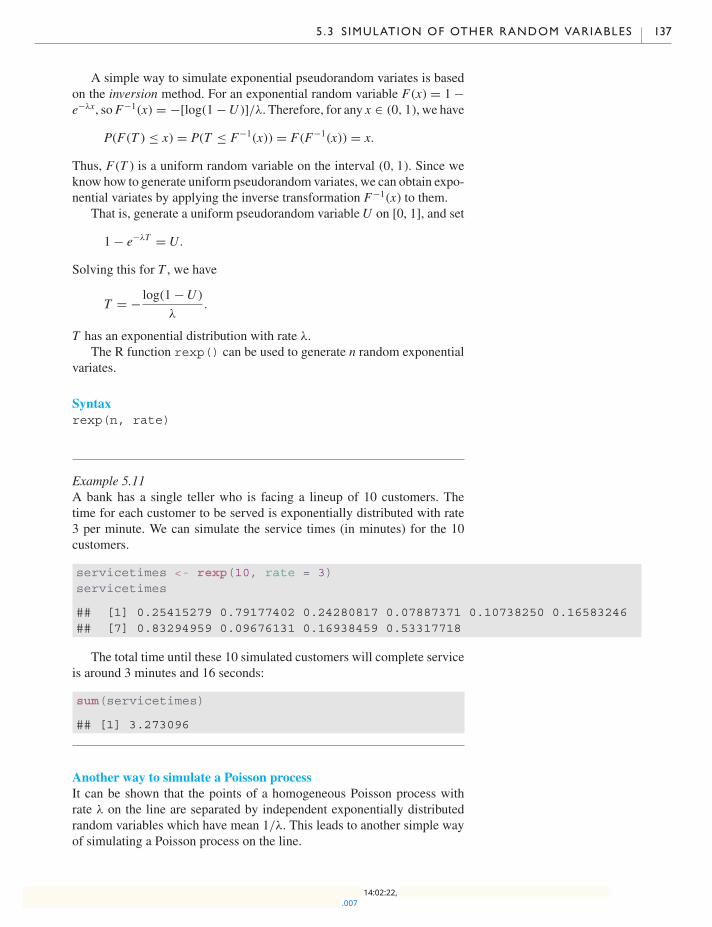
5 .3 S IMULATION OF OTHER RANDOM VARIABLES 137
A simple way to simulate exponential pseudorandom variates is basedon the inversion method. For an exponential random variable F (x) = 1 −e−λx, soF−1(x) = −[log(1 −U )]/λ. Therefore, for any x ∈ (0, 1), we have
P(F (T ) ≤ x) = P(T ≤ F−1(x)) = F (F−1(x)) = x.
Thus, F (T ) is a uniform random variable on the interval (0, 1). Since weknow how to generate uniform pseudorandom variates, we can obtain expo-nential variates by applying the inverse transformation F−1(x) to them.
That is, generate a uniform pseudorandom variableU on [0, 1], and set
1 − e−λT = U.
Solving this for T , we have
T = − log(1 −U )
λ.
T has an exponential distribution with rate λ.The R function rexp() can be used to generate n random exponential
variates.
Syntaxrexp(n, rate)
Example 5.11A bank has a single teller who is facing a lineup of 10 customers. Thetime for each customer to be served is exponentially distributed with rate3 per minute. We can simulate the service times (in minutes) for the 10customers.
servicetimes <- rexp(10, rate = 3)servicetimes
## [1] 0.25415279 0.79177402 0.24280817 0.07887371 0.10738250 0.16583246## [7] 0.83294959 0.09676131 0.16938459 0.53317718
The total time until these 10 simulated customers will complete serviceis around 3 minutes and 16 seconds:
sum(servicetimes)
## [1] 3.273096
Another way to simulate a Poisson processIt can be shown that the points of a homogeneous Poisson process withrate λ on the line are separated by independent exponentially distributedrandom variables which have mean 1/λ. This leads to another simple wayof simulating a Poisson process on the line.
.00714:02:22,
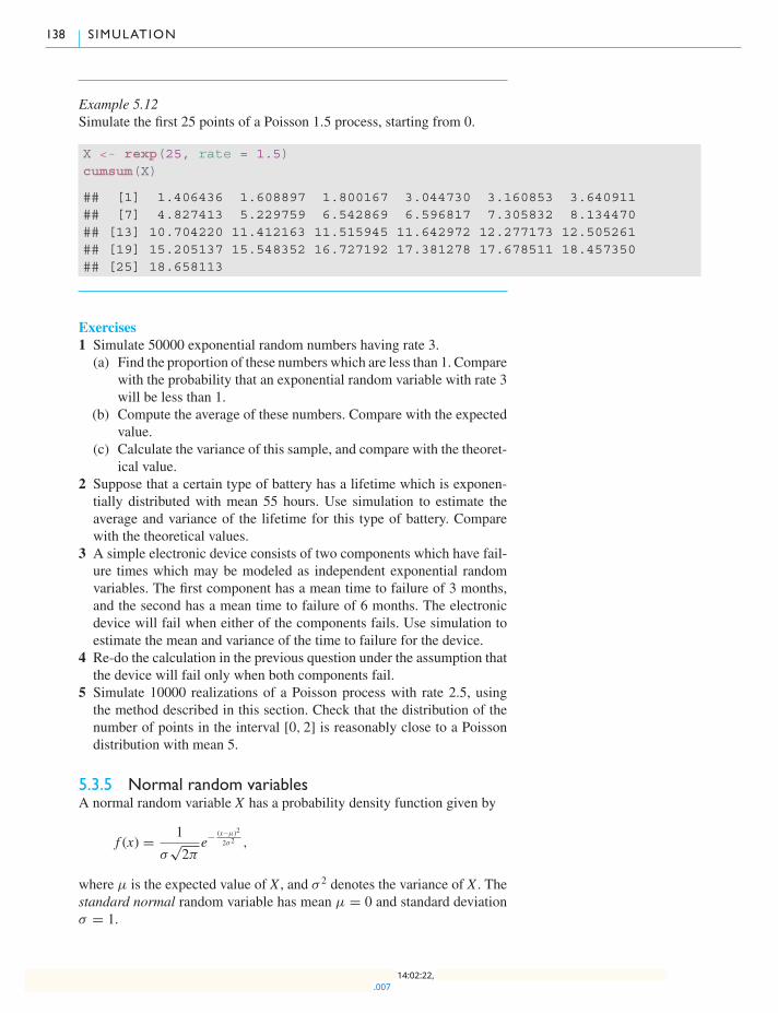
138 S IMULATION
Example 5.12Simulate the first 25 points of a Poisson 1.5 process, starting from 0.
X <- rexp(25, rate = 1.5)cumsum(X)
## [1] 1.406436 1.608897 1.800167 3.044730 3.160853 3.640911## [7] 4.827413 5.229759 6.542869 6.596817 7.305832 8.134470## [13] 10.704220 11.412163 11.515945 11.642972 12.277173 12.505261## [19] 15.205137 15.548352 16.727192 17.381278 17.678511 18.457350## [25] 18.658113
Exercises1 Simulate 50000 exponential random numbers having rate 3.(a) Find the proportion of these numbers which are less than 1. Compare
with the probability that an exponential random variable with rate 3will be less than 1.
(b) Compute the average of these numbers. Compare with the expectedvalue.
(c) Calculate the variance of this sample, and compare with the theoret-ical value.
2 Suppose that a certain type of battery has a lifetime which is exponen-tially distributed with mean 55 hours. Use simulation to estimate theaverage and variance of the lifetime for this type of battery. Comparewith the theoretical values.
3 A simple electronic device consists of two components which have fail-ure times which may be modeled as independent exponential randomvariables. The first component has a mean time to failure of 3 months,and the second has a mean time to failure of 6 months. The electronicdevice will fail when either of the components fails. Use simulation toestimate the mean and variance of the time to failure for the device.
4 Re-do the calculation in the previous question under the assumption thatthe device will fail only when both components fail.
5 Simulate 10000 realizations of a Poisson process with rate 2.5, usingthe method described in this section. Check that the distribution of thenumber of points in the interval [0, 2] is reasonably close to a Poissondistribution with mean 5.
5.3.5 Normal random variablesA normal random variable X has a probability density function given by
f (x) = 1
σ√2π
e−(x−μ)2
2σ2 ,
where μ is the expected value of X , and σ 2 denotes the variance of X . Thestandard normal random variable has mean μ = 0 and standard deviationσ = 1.
.00714:02:22,
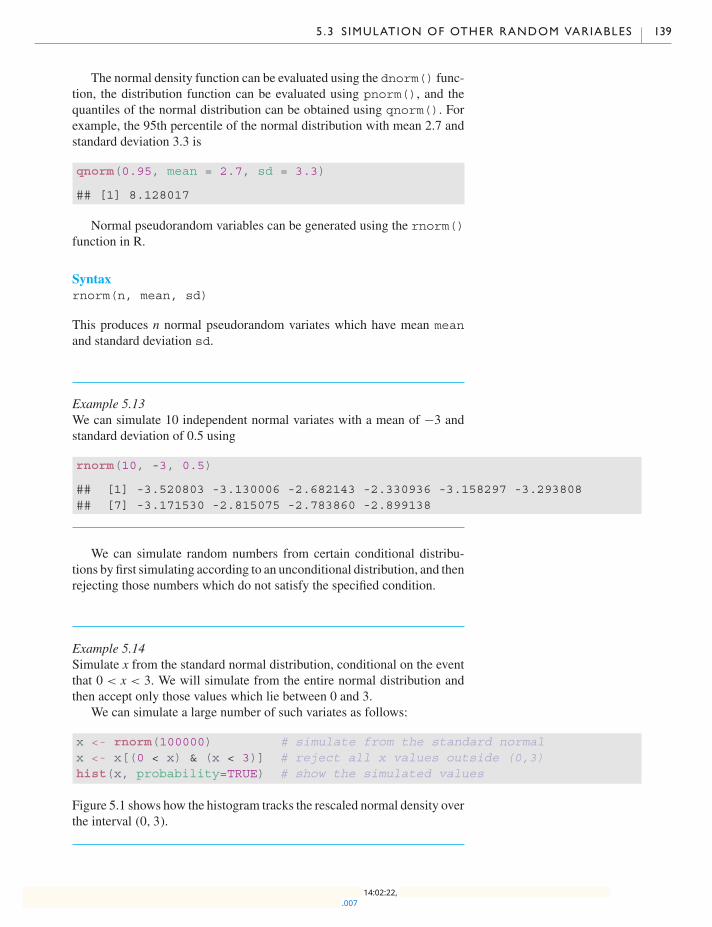
5 .3 S IMULATION OF OTHER RANDOM VARIABLES 139
The normal density function can be evaluated using the dnorm() func-tion, the distribution function can be evaluated using pnorm(), and thequantiles of the normal distribution can be obtained using qnorm(). Forexample, the 95th percentile of the normal distribution with mean 2.7 andstandard deviation 3.3 is
qnorm(0.95, mean = 2.7, sd = 3.3)
## [1] 8.128017
Normal pseudorandom variables can be generated using the rnorm()function in R.
Syntaxrnorm(n, mean, sd)
This produces n normal pseudorandom variates which have mean meanand standard deviation sd.
Example 5.13We can simulate 10 independent normal variates with a mean of −3 andstandard deviation of 0.5 using
rnorm(10, -3, 0.5)
## [1] -3.520803 -3.130006 -2.682143 -2.330936 -3.158297 -3.293808## [7] -3.171530 -2.815075 -2.783860 -2.899138
We can simulate random numbers from certain conditional distribu-tions by first simulating according to an unconditional distribution, and thenrejecting those numbers which do not satisfy the specified condition.
Example 5.14Simulate x from the standard normal distribution, conditional on the eventthat 0 < x < 3. We will simulate from the entire normal distribution andthen accept only those values which lie between 0 and 3.
We can simulate a large number of such variates as follows:
x <- rnorm(100000) # simulate from the standard normalx <- x[(0 < x) & (x < 3)] # reject all x values outside (0,3)hist(x, probability=TRUE) # show the simulated values
Figure 5.1 shows how the histogram tracks the rescaled normal density overthe interval (0, 3).
.00714:02:22,

140 S IMULATION
Histogram of x
x
Den
sity
0.0 0.5 1.0 1.5 2.0 2.5 3.0
0.0
0.2
0.4
0.6
0.8
Fig. 5.1 Histogram of simulatedvalues with the standard normaldensity (solid curve) and therescaled normal density (dashedcurve) overlaid.
5.3.6 All built-in distributionsThere are many standard distributions built into R. These follow a generalnaming convention: rXXXX generates random values, dXXXX gives the den-sity or probability function, pXXXX gives the cumulative distribution func-tion, and qXXXX gives the quantiles. Table 5.1 lists many of the univariatecontinuous distributions, and Table 5.2 lists many of the univariate discretedistributions. For simplicity, the normalizing constants in the densities andprobability functions have been omitted.
Exercises1 Simulate 100 realizations of a normal random variable having mean 51and standard deviation 5.2. Estimate the mean and standard deviation ofyour simulated sample and compare with the theoretical values.
2 Simulate 1000 realizations of a standard normal random variable Z, anduse your simulated sample to estimate(a) P(Z > 2.5),(b) P(0 < Z < 1.645),(c) P(1.2 < Z < 1.45),(d) P(−1.2 < Z < 1.3).Compare with the theoretical values.
3 Simulate from the conditional distribution of a normal random variableX with mean 3 and variance 16, given that |X | > 2.
4 Using the fact that a χ2 random variable on one degree of freedom hasthe same distribution as the square of a standard normal random variable,simulate 100 independent realizations of such a χ2 random variable, andestimate its mean and variance. (Compare with the theoretical values: 1,2.)
5 A χ2 random variable on n degrees of freedom has the same distributionas the sum of n independent standard normal random variables. Simulatea χ2 random variable on eight degrees of freedom, and estimate its meanand variance. (Compare with the theoretical values: 8, 16.)
.00714:02:22,
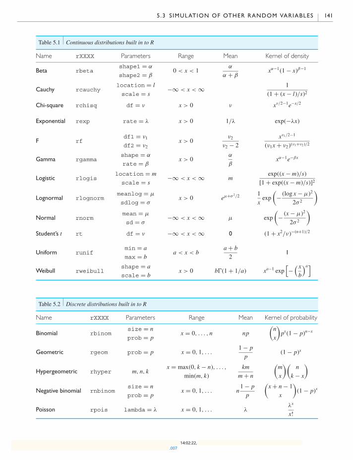
5 .3 S IMULATION OF OTHER RANDOM VARIABLES 141
Table 5.1 Continuous distributions built in to R
Name rXXXX Parameters Range Mean Kernel of density
Beta rbetashape1 = α
shape2 = β0 < x < 1
α
α + βxα−1(1 − x)β−1
Cauchy rcauchylocation = l
scale = s−∞ < x < ∞ 1
(1 + (x− l)/s)2
Chi-square rchisq df = ν x > 0 ν xν/2−1e−x/2
Exponential rexp rate = λ x > 0 1/λ exp(−λx)
F rfdf1 = ν1
df2 = ν2x > 0
ν2
ν2 − 2
xν1/2−1
(ν1x+ ν2)(ν1+ν2 )/2
Gamma rgammashape = α
rate = βx > 0
α
βxα−1e−βx
Logistic rlogislocation = m
scale = s−∞ < x < ∞ m
exp((x− m)/s)
[1 + exp((x− m)/s)]2
Lognormal rlognormmeanlog = μ
sdlog = σx > 0 eμ+σ 2/2 1
xexp
(− (log x− μ)2
2σ 2
)Normal rnorm
mean = μ
sd = σ−∞ < x < ∞ μ exp
(− (x− μ)2
2σ 2
)Student’s t rt df = ν −∞ < x < ∞ 0 (1 + x2/ν)−(n+1)/2
Uniform runifmin = a
max = ba < x < b
a+ b
21
Weibull rweibullshape = a
scale = bx > 0 b(1 + 1/a) xa−1 exp
[−
( xb
)a]
Table 5.2 Discrete distributions built in to R
Name rXXXX Parameters Range Mean Kernel of probability
Binomial rbinomsize = n
prob = px = 0, . . . , n np
(n
x
)px(1 − p)n−x
Geometric rgeom prob = p x = 0, 1, . . .1 − p
p(1 − p)x
Hypergeometric rhyper m, n, kx = max(0, k − n), . . . ,
min(m, k)
km
m+ n
(m
x
)(n
k − x
)Negative binomial rnbinom
size = n
prob = px = 0, 1, . . . n
1 − p
p
(x+ n− 1
x
)(1 − p)x
Poisson rpois lambda = λ x = 0, 1, . . . λλx
x!
.00714:02:22,
142 S IMULATION
5.4 Multivariate random number generation
Most interesting problems in statistics and applied probability don’t involvejust one random value, they will involve several values that are related. Rhas a few multivariate distributions built in, but in many cases users need toconstruct their own simulations. There are many techniques for doing this.We will describe just one: sequential conditional generation.
The idea of this technique is that even if X = (X1,X2, . . . ,Xp) has acomplicated p-dimensional distribution, X1 will have a one-dimensionalmarginal distribution. So we start by simulating just X1, then simulate X2from its conditional distribution given X1, and X3 conditional on X1 and X2,and so on. If it is difficult to calculate marginal and conditional distributionsthen this might not be feasible, but in a surprising number of cases, it is not.
Example 5.15A model commonly used in financial engineering says that the price of astock Xt+1 at the close of trading on day t + 1 is equal to the closing priceXt on the previous day, multiplied by a value whose logarithm has a normaldistribution. The multipliers are independent from day to day.
Suppose a stock starts at $100.00 per share, and we expect a 1% changein price from one day to the next. What would be the joint distribution ofthe prices over the next five days? What is the probability that it remainsabove $100 on all five days?
We can simulate this by starting with X0 = 100, and multiplying byexp(Zt ), where Zt , t = 1, . . . , 5 are independent normal random vari-ables with mean 0 and standard deviation of log(1.01). We do this in areplicate() loop to get 1000 examples of the simulation:
X <- numeric(6)X[1] <- 100results <- replicate(1000, {
for (t in 1:5)X[t + 1] <- X[t] * exp(rnorm(1, mean = 0, sd = log(1.01)))
X})str(results)
## num [1:6, 1:1000] 100 101.1 100 98.1 98.1 ...
We see that they have been returned in a matrix with 6 rows and 1000columns. How many of those cases have all values greater than 100?
table(apply(results, 2, function(x) all(x[2:6] > 100)))
#### FALSE TRUE## 749 251
We see that it happens about a quarter of the time.
.00714:02:22,
5 .5 MARKOV CHAIN SIMULATION 143
5.5 Markov chain simulation
Markov chains are sequences of random variables X0,X1, . . . where thedistribution of Xt+1, conditional on all previous values, depends only onXt . They are commonly used in modeling systems with short memories,such as the stock market, where the price tomorrow is modeled to dependonly on the price today, biological systems where the genome of the off-spring depends only on the genome of the parents, etc. When Xt is a dis-crete random variable with a finite number of states 1, . . . , n, it is conve-nient to represent the conditional distributions in an n× n matrix P, whereentry Pi j holds the conditional probability that Xt+1 = j given that Xt = i.Because probabilities sum to 1, we have row sums
∑nj=1 Pi j = 1 for all
i = 1, . . . , n.Simulation of such Markov chains in R is easy using the sequential
conditional simulation method that was described in the previous section.The value of Xt+1 is simply the value drawn by
sample(1:n, size = 1, prob = P[X[t], ])
An interesting fact about Markov chains is that they have an invariantdistribution, i.e. a distribution P(Xt = i) = πi such that if Xt is drawn fromthe invariant distribution and updated using the Pmatrix, then the marginaldistribution of Xt+1 will also be the invariant distribution. (For some P,there will be more than one invariant distribution, but there is always atleast one.) Even more interesting is the fact that for some P matrices, if X0is drawn from any distribution, then the marginal distribution of Xt for larget approximates the invariant distribution. This is used in methods calledMarkov chain Monte Carlo (or MCMC) to draw values with distributionclose to πi even when πi can’t be calculated directly.
Example 5.16Consider a model of a disease with three stages. Stage 1 is healthy, stage2 is mild disease, and stage 3 is severe disease. Healthy individuals remainhealthy with probability 0.99 and develop mild disease with probability0.01. Individuals with mild disease are cured and become healthy withprobability 0.5, remain with mild disease with probability 0.4, and progressto serious disease with probability 0.1. Finally, those with severe diseasestay in that state with probability 0.75, and improve to mild disease withprobability 0.25.
This describes a Markov chain with three states, and
P =
⎡⎢⎣0.99 0.01 0.00
0.50 0.40 0.10
0.00 0.25 0.75
⎤⎥⎦ .
We will simulate two individuals for 10000 steps: one who starts healthy,and one who starts with severe disease:
.00714:02:22,

144 S IMULATION
P <- matrix(c(0.99, 0.01, 0,0.5, 0.4, 0.1,0, 0.25, 0.75), 3, 3, byrow = TRUE)
healthy <- numeric(10000)healthy[1] <- 1for (t in 1:9999)
healthy[t + 1] <- sample(1:3, size = 1, prob = P[healthy[t], ])table(healthy)
## healthy## 1 2 3## 9692 218 90
sick <- numeric(10000)sick[1] <- 3for (t in 1:9999)
sick[t + 1] <- sample(1:3, size = 1, prob = P[sick[t], ])table(sick)
## sick## 1 2 3## 9646 216 138
We see that the two individuals have very similar distributions of statesover the 10000 steps. In fact, their distribution is close to the (unique)invariant distribution for P, which can be shown by other means (see Chap-ter exercise 1 in Chapter 6) to be approximately (0.973, 0.020, 0.008).
Example 5.17The tune for L. van Beethoven’s Ode to Joy can be represented in “Lily-pond” format, a standard format for representing musical scores on a com-puter, as follows:
\score{{\tempo 4 = 120e’4 e’4 f’4 g’4 g’4 f’4 e’4 d’4 c’4 c’4 d’4 e’4 e’4. d’8 d’2e’4 e’4 f’4 g’4 g’4 f’4 e’4 d’4 c’4 c’4 d’4 e’4 d’4. c’8 c’2d’4 d’4 e’4 c’4 d’4 e’8 f’8 e’4 c’4 d’4 e’8 f’8 e’4 d’4 c’4 d’4 g2e’4 e’4 f’4 g’4 g’4 f’4 e’4 d’4 c’4 c’4 d’4 e’4 d’4. c’8 c’2}\layout{}\midi{}
}
The actual music starts on the fourth line; each note is represented bysymbols containing two parts: a letter for the pitch, and a number for theduration. The punctuation marks modify the pitch or duration. This filecan be converted to standard musical notation or to a “MIDI” file which
.00714:02:22,

5 .5 MARKOV CHAIN SIMULATION 145
can be played on most computers. At the time of writing, the websitehttp://lilybin.com contains online tools to do this.
We can compose music with some of the characteristics of the Ode toJoy by randomly sampling the same set of symbols with R. First, we savethe lines to a file ode.ly, and read the symbols into a character vector,with one symbol per element:
notes <- scan("ode.ly", skip = 3, nlines = 4, what = character())
We can randomly sample notes and write the results to a file using thefollowing code:
random <- sample(notes, 63, replace = TRUE)
writeLilypond <- function(notes, filename = "") {cat(c("\\score{\n {\n \\tempo 4 = 120",
paste(" ", strwrap(paste(notes, collapse = " ")))," }\n \\layout{}\n \\midi{}\n}"),
sep = "\n", file = filename)}
writeLilypond(random, filename = "indep.txt")
This gives a pleasant sound, but it’s not much like Beethoven. We can makeit more like the original by sampling from a Markov chain with transitionprobabilities similar to the original. But it would be nice to keep even moreof the characteristics, for example having the selection of notes match theoriginal frequencies conditional on two previous notes, not just one. Thatis, we would like the distribution of noteYt to depend on bothYt−1 andYt−2.
It turns out we can do this, and still have a Markov chain. Define Zt =(Yt−1,Yt ). Then Zt is a Markov chain from which we can extract Yt easily.We can generalize this to allow Yt to depend on n previous observations.
One practical problem with simulating a process like this is that if Ythas m states, then Zt has mn states. Our sample song has 14 different notes;if we want to match the distribution for 5 consecutive notes, we’d need145 = 537824 different possible states for Zt , and the transition matrix Pfor Zt might be too large tomanage. However, thePmatrix will be “sparse”:most entries will be zero. For example, our song has only 61 transitions,with some repetition. It is easy to represent this sparse matrix, but we uselist(), not matrix(). The following function counts the transitions inthe original data:
countTransitions <- function(notes, n) {len <- length(notes)# Put special markers at the start and endnotes <- c(rep("START", n), notes, "STOP")result <- list(n = n)# Loop over the data + STOP, counting symbolsfor (i in 1:(len+1)) {index <- notes[ seq_len(n+1) + i - 1 ]# We store only positive results, so if we’ve never seen this
.00714:02:22,

146 S IMULATION
# transition before, it will be NULL; insert an empty list()for (j in seq_len(n)) {if (is.null(result[[ index[1:j] ]]))result[[ index[1:j] ]] <- list()
}prevcount <- result[[ index ]]if (is.null(prevcount))result[[ index ]] <- 1
elseresult[[ index ]] <- result[[ index ]] + 1
}result
}
This returns the result in a list that records n. We can use this list to generatenew music using this function:
generateTransitions <- function(counts, len, filename = "") {# Initialize with STARTn <- counts$nlen <- len + nnotes <- rep("START", len)i <- nwhile (i < len && notes[i] != "STOP" ) {
i <- i + 1index <- notes[i - n:1]distn <- counts[[ index ]]notes[i] <- sample(names(distn), 1, prob = distn)
}# Now leave off START and STOP, and return the resultnotes[ !(notes %in% c("START", "STOP")) ]
}
Here we give a maximum length, but if we reach the STOP marker, westop early. Using these functions with n = 2 produces this output, which isshown in standard musical notation in Figure 5.2:
counts <- countTransitions(notes, 2)writeLilypond(generateTransitions(counts, 100))
\score{{\tempo 4 = 120e’4 e’4 f’4 g’4 g’4 f’4 e’4 d’4 c’4 c’4 d’4 e’4 c’4 d’4 e’4e’4. d’8 d’2 e’4 e’4 f’4 g’4 g’4 f’4 e’4 d’4 c’4 c’4 d’4 e’4e’4. d’8 d’2 e’4 e’4 f’4 g’4 g’4 f’4 e’4 d’4 c’4 c’4 d’4 e’4d’4. c’8 c’2}\layout{}\midi{}
}
.00714:02:22,
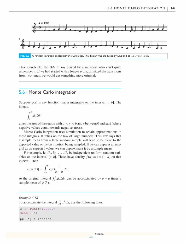
5 .6 MONTE CARLO INTEGRATION 147
Fig. 5.2 A random variation on Beethoven’s Ode to Joy. The display was produced by Lilypond on lilybin.com.
This sounds like the Ode to Joy played by a musician who can’t quiteremember it. If we had started with a longer score, or mixed the transitionsfrom two tunes, we would get something more original.
5.6 Monte Carlo integration
Suppose g(x) is any function that is integrable on the interval [a, b]. Theintegral∫ b
ag(x)dx
gives the area of the region with a < x < b and y between 0 and g(x) (wherenegative values count towards negative areas).
Monte Carlo integration uses simulation to obtain approximations tothese integrals. It relies on the law of large numbers. This law says thata sample mean from a large random sample will tend to be close to theexpected value of the distribution being sampled. If we can express an inte-gral as an expected value, we can approximate it by a sample mean.
For example, let U1,U2, . . . ,Un be independent uniform random vari-ables on the interval [a, b]. These have density f (u) = 1/(b− a) on thatinterval. Then
E[g(Ui)] =∫ b
ag(u)
1
b− adu,
so the original integral∫ ba g(x)dx can be approximated by b− a times a
sample mean of g(Ui).
Example 5.18To approximate the integral
∫ 10 x
4 dx, use the following lines:
u <- runif(100000)mean(uˆ4)
## [1] 0.2005908
.00714:02:22,

148 S IMULATION
Compare the exact answer 0.2, which can easily be computed in thiscase.
Example 5.19To approximate the integral
∫ 52 sin(x)dx, use the following lines:
u <- runif(100000, min = 2, max = 5)mean(sin(u))*(5-2)
## [1] -0.6851379
The true value can be shown to be −0.700.
Multiple integrationNow letV1,V2, . . . ,Vn be an additional set of independent uniform randomvariables on the interval [0, 1], and suppose g(x, y) is now an integrablefunction of the two variables x and y. The law of large numbers says that
limn→∞
n∑i=1
g(Ui,Vi)/n =∫ 1
0
∫ 1
0g(x, y)dx dy
with probability 1.So we can approximate the integral
∫ 10
∫ 10 g(x, y)dx dy by generat-
ing two sets of independent uniform pseudorandom variates, computingg(Ui,Vi) for each one, and taking the average.
Example 5.20Approximate the integral
∫ 103
∫ 71 sin(x− y)dx dy using the following:
U <- runif(100000, min = 1, max = 7)V <- runif(100000, min = 3, max = 10)mean(sin(U - V))*42
## [1] 0.07989664
The factor of 42 = (7 − 1)(10 − 3) compensates for the joint densityofU and V being f (u, v ) = 1/42.
The uniform density is by no means the only density that can be used inMonte Carlo integration. If the density of X is f (x), then E[g(X )/ f (X )] =∫[g(x)/ f (x)] f (x)dx = ∫
g(x)dx so we can approximate the latter by sam-ple averages of g(X )/ f (X ).
.00714:02:22,
5 .7 ADVANCED SIMULATION METHODS 149
Example 5.21To approximate the integral
∫ ∞1 exp(−x2)dx, write it as
∫ ∞0 exp[−(x+
1)2]dx, and use an exponential distribution for X :
X <- rexp(100000)mean( exp( -(X + 1)ˆ2 ) / dexp(X) )
## [1] 0.140112
The true value of this integral is 0.1394.
Monte Carlo integration is not always successful: sometimes the ratiog(X )/ f (X ) varies so much that the sample mean doesn’t converge. Try tochoose f (x) so this ratio is roughly constant, and avoid situations whereg(x)/ f (x) can be arbitrarily large.
Exercises1 Use Monte Carlo integration to estimate the following integrals. Com-pare with the exact answer, if known.∫ 1
0x dx,
∫ 3
1x2 dx,
∫ π
0sin(x)dx,
∫ π
1ex dx,
∫ ∞
0e−x dx,∫ ∞
0e−x
3dx,
∫ 3
0sin(ex)dx,
∫ 1
0
1√2π
e−x2/2 dx,
∫ 2
0
1√2π
e−x2/2 dx,
∫ 3
0
1√2π
e−x2/2 dx.
2 Use Monte Carlo integration to estimate the following double integrals.∫ 1
0
∫ 1
0cos(x− y)dx dy,
∫ 1
0
∫ 1
0e−(y+x)2 (x+ y)2 dx dy,∫ 3
0
∫ 1
0cos(x− y)dx dy,
∫ 5
0
∫ 2
0e−(y+x)2 (x+ y)2 dx dy.
5.7 Advanced simulation methods
The simulation methods discussed so far will work only for particular typesof probability densities or distributions. General purpose simulation meth-ods can be used to draw pseudorandom samples from a wide variety ofdistributions.
Example 5.22Suppose X is a Binomial(n, p) random variable with n known, but wherethe value of p is not known precisely; it is near 0.7. Given the data valueX = x, we want to estimate p.
.00714:02:22,

150 S IMULATION
−1 0 1 2 30.
00.
40.
8x
1−|1
−x|
−1 0 1 2 3
0.0
0.4
0.8
x
1−|1
−x|
Fig. 5.3 The graph of thetriangular density function on(0, 2), together with a dashedrectangle in the right hand panel.
The maximum likelihood estimator for p is p = x/n, but this ignoresour prior knowledge, i.e. the fact that p is really near 0.7.
If we convert our prior knowledge to a density, e.g., p ∼ N(0.7, σ =0.1), Bayes’ theorem lets us calculate the conditional density of p, givenX = x, as
f (p |X = x) ∝ exp
(−(p− 0.7)2
2(0.1)2
)px(1 − p)n−x, 0 < p < 1.
It is quite difficult to work out the constant that makes this a standard den-sity integrating to 1, but numerical approximations (e.g. using Monte Carlointegration) are possible.
The goal of the remainder of this section is to present simulation meth-ods which can be used to generate pseudorandom numbers from a densitylike the one in the above example. Two simulation methods are commonlyused:
� rejection sampling� importance sampling
5.7.1 Rejection samplingThe idea of rejection sampling was used in Section 5.3.5 to sample from aconditional distribution: sample from a convenient distribution, and selecta subsample to achieve the target distribution. We will show how to userejection sampling to draw a random sample from a univariate density orprobability function g(x), using a sequence of two examples.
Our first example demonstrates the simplest version of rejectionsampling.
Example 5.23Simulate pseudorandom variates from the triangular density function
g(x) ={1 − |1 − x|, 0 ≤ x < 2,0, otherwise.
The graph of the density function is displayed in the left panel ofFigure 5.3. If we could draw points uniformly from the triangular regionbelow the density, the x-coordinate would be distributed with density g(x).
.00714:02:22,
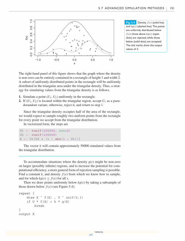
5 .7 ADVANCED SIMULATION METHODS 151
−1.0 −0.5 0.0 0.5 1.0
0.0
0.2
0.4
0.6
0.8
1.0
x
f(x)
Fig. 5.4 Density f (x) (solid line)and kg(x) (dashed line). The pointsare uniformly distributed belowf (x); those above kg(x) (opendots) are rejected, while thosebelow (solid dots) are accepted.The tick marks show the outputvalues of X .
The right-hand panel of this figure shows that the graph where the densityis non-zero can be entirely contained in a rectangle of height 1 and width 2.A subset of uniformly distributed points in the rectangle will be uniformlydistributed in the triangular area under the triangular density. Thus, a strat-egy for simulating values from the triangular density is as follows.
1. Simulate a point (U1,U2) uniformly in the rectangle.2. If (U1,U2) is located within the triangular region, accept U1 as a pseu-
dorandom variate; otherwise, reject it, and return to step 1.
Since the triangular density occupies half of the area of the rectangle,we would expect to sample roughly two uniform points from the rectanglefor every point we accept from the triangular distribution.
In vectorized form, the steps are
U1 <- runif(100000, max=2)U2 <- runif(100000)X <- U1[U2 < (1 - abs(1 - U1))]
The vector X will contain approximately 50000 simulated values fromthe triangular distribution.
To accommodate situations where the density g(x) might be non-zeroon larger (possibly infinite) regions, and to increase the potential for com-putational efficiency, a more general form of rejection sampling is possible.Find a constant k, and density f (x) from which we know how to sample,and for which kg(x) ≤ f (x) for all x.
Then we draw points uniformly below kg(x) by taking a subsample ofthose drawn below f (x) (see Figure 5.4):
repeat {draw X ˜ f(X) , U ˜ unif(0,1)if U * f(X) < k * g(X)
break}output X
.00714:02:22,
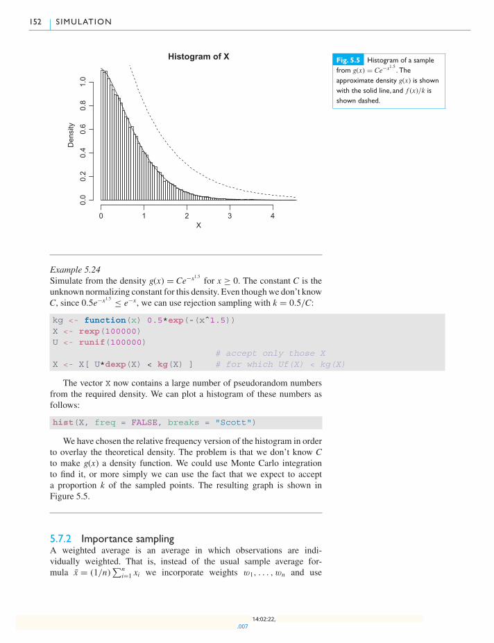
152 S IMULATION
Histogram of X
X
Den
sity
0 1 2 3 4
0.0
0.2
0.4
0.6
0.8
1.0
Fig. 5.5 Histogram of a samplefrom g(x) = Ce−x1.5 . Theapproximate density g(x) is shownwith the solid line, and f (x)/k isshown dashed.
Example 5.24Simulate from the density g(x) = Ce−x
1.5for x ≥ 0. The constant C is the
unknown normalizing constant for this density. Even thoughwe don’t knowC, since 0.5e−x
1.5 ≤ e−x, we can use rejection sampling with k = 0.5/C:
kg <- function(x) 0.5*exp(-(xˆ1.5))X <- rexp(100000)U <- runif(100000)
# accept only those XX <- X[ U*dexp(X) < kg(X) ] # for which Uf(X) < kg(X)
The vector X now contains a large number of pseudorandom numbersfrom the required density. We can plot a histogram of these numbers asfollows:
hist(X, freq = FALSE, breaks = "Scott")
We have chosen the relative frequency version of the histogram in orderto overlay the theoretical density. The problem is that we don’t know Cto make g(x) a density function. We could use Monte Carlo integrationto find it, or more simply we can use the fact that we expect to accepta proportion k of the sampled points. The resulting graph is shown inFigure 5.5.
5.7.2 Importance samplingA weighted average is an average in which observations are indi-vidually weighted. That is, instead of the usual sample average for-mula x = (1/n)
∑ni=1 xi we incorporate weights w1, . . . ,wn and use
.00714:02:22,
5 .7 ADVANCED SIMULATION METHODS 153
xw = ∑ni=1 wixi/
∑ni=1 wi. The usual sample average can be seen to be a
weighted average with all weights equal.Importance sampling is a technique to generate both the sample and
the weights randomly, in such a way that weighted averages approximateexpected values with respect to a target density function g(x). As with rejec-tion sampling, we start by sampling from some other more convenient den-sity f (x).
1. Choose a convenient density f (x) (which we know how to draw samplesfrom).
2. Draw (x1, . . . , xn) as a sample from f (x).3. Calculate weights wi = g(xi)/ f (xi).
We may now approximate the expectation of a function h(X ) whereX ∼ g(x) using averages of h(xi) weighted by wi.
One way to see why this works is to notice that wi is proportional to theprobability that a rejection sampler would accept xi as a draw from g(x).Given xi, the contribution wih(xi)/
∑ni=1 wi in the weighted average for-
mula is exactly the expected contribution from this draw to a sample meanif we were using rejection sampling. We know rejection sampling works,so importance sampling must work too. It may even be more efficient, inthat we don’t throw away information from rejected draws. In addition, it isnot necessary to find the constant k as in rejection sampling. Neither g(xi)nor f (xi) need be normalized densities: dividing by the sum of the weightsautomatically provides the appropriate scaling.
On the other hand, workingwithweighted samples is more difficult thanworking with simple random samples, so in many cases rejection samplingwould be preferred.
We illustrate these issues by continuing with the example from the pre-vious section. We may approximate the mean and variance of the densityg(x) from that section using the weighted.mean function:
X <- rexp(100000)W <- g(X)/dexp(X)mean <- weighted.mean(X, W)mean
## [1] 0.6579574
weighted.mean( (X - mean)ˆ2, W ) # The variance as E[ (X - Xbar)ˆ2 ]
## [1] 0.3036045
Exercises1 Write a function to generate standard normal pseudorandom numbers onthe interval [−4, 4], using runif() and the rejection method. Can youmodify the function so that it can generate standard normal pseudoran-dom numbers on the entire real line?
.00714:02:22,
154 S IMULATION
2 The following function returns normal pseudorandom numbers:
rannorm <- function(n, mean = 0, sd = 1){singlenumber <- function() {
repeat{U <- runif(1)U2 <- sign(runif(1, min = -1)) # value is +1 or -1Y <- rexp(1) * U2 # Y is a double exponential r.v.if (U < dnorm(Y) / exp(-abs(Y))) break
}return(Y)
}replicate(n, singlenumber()) * sd + mean
}
(a) Use this function to generate a vector of 10000 normal pseudoran-dom numbers with mean 8 and standard deviation 2.
(b) Obtain a QQ plot to check the accuracy of this generator.(c) Use the curve() function to draw the graph of the standard normal
density on the interval [0, 4]. Use the add = TRUE parameter tooverlay the exponential density on the same interval to verify thatthe rejection method has been implemented appropriately.
3 Consider the following twomethods for simulating from the discrete dis-tribution with values 0, 1, 2, 3, 4, 5 which take respective probabilities0.2, 0.3, 0.1, 0.15, 0.05, 0.2.
The first method is an inversion method:
probs <- c(0.2, 0.3, 0.1, 0.15, 0.05, 0.2)randiscrete1 <- function(n, probs) {
cumprobs <- cumsum(probs)singlenumber <- function() {
x <- runif(1)N <- sum(x > cumprobs)N
}replicate(n, singlenumber())
}
The second method is a rejection method:
randiscrete2 <- function(n, probs) {singlenumber <- function() {
repeat{U <- runif(2, min=c(-0.5, 0), max=c(length(probs) - 0.5,
max(probs)))if (U[2] < probs[round(U[1]) + 1]) break
}return(round(U[1]))
}replicate(n, singlenumber())
}
.00714:02:22,
CHAPTER EXERCISES 155
Execute both functions using n = 100, 1000, and 10000. Usesystem.time() to determine which method is faster.
4 Repeat the above exercise using the probability distribution on the inte-gers {0, 1, 2, . . . , 99} defined by
set.seed(91626)probs <- runif(100)probs <- probs / sum(probs)
When is rejection sampling preferred to the inversionmethod for discretedistributions?
5 Write a function which generates a weighted sample of binomial(m, p) pseudorandom numbers using importance sampling. Compare theweighted average with the theoretical mean.
Chapter exercises1 Write a function which simulates two people (Ann and Bob) playingtable tennis. (Assume that the first person to reach 21 points wins thegame.)(a) Begin with the assumption that each player successively hits the ball
with probability pAnn and pBob, respectively. Find the probabilitythat Ann will win for various values of these probabilities.
(b) Add more features such as ability to serve, to smash the ball, or spinthe ball. Use your imagination.
2 (Adapted fromElementary Probability Theory with Stochastic Processesby K. L. Chung, Springer, 1975.) The following model has been used forthe study of contagion. Suppose that there are N persons, some of whomare sick with influenza. The following assumptions are made:� when a sick person meets a healthy one, the chance that the latter willbe infected is α;
� all encounters are between two persons;� all possible encounters in pairs are equally likely;� one such encounter occurs in every unit of time.(a) Write a function which simulates this model for various values of N
(say, 10000) and α (say, between 0.001 and 0.1). Monitor the his-tory of this process, assuming that one individual is infected at thebeginning.
(b) Suppose that initially only one individual is infected. What is theexpected length of time until 1000 people are infected?
(c) Now add the assumption that each infected person has a 0.01 chanceof recovering at each time unit. Monitor several histories of this newprocess, and compare them with the histories of the old process.
(d) Re-do with the assumption that the time between encounters is anexponential random variable with mean 5 minutes.
(e) Re-do assuming that the time between encounters is the absolutevalue of a normal random variable with a mean of 5 minutes and astandard deviation of 1 minute.
3 Simulate the following simple model of auto insurance claims.� Claims arise according to a Poisson process at a rate of 100 per year.
.00714:02:22,

156 S IMULATION
� Each claim is a random size following a gamma distributionwith shapeand rate parameters both equal to 2. This distribution has mean 1 andvariance 1/2. Claims must be paid by the insurance company as soonas they arise.
� The insurance company earns premiums at a rate of 105 per year,spread evenly over the year (i.e. at time t measured in years, the totalpremium received is 105t).Write R code to do the following.
(a) Simulate the times and amounts of all the claims that would occurin one year. Draw a graph of the total amount of money that theinsurance company would have through the year, starting from zero:it should increase smoothly with the premiums, and drop at eachclaim time.
(b) Repeat the simulation 1000 times, and estimate the followingquantities.(i) The expected minimum amount of money that the insurance
company would have.(ii) The expected final amount ofmoney that the insurance company
would have.4 Let f (x) = (sin x)2 for 0 < x < 2π .
(a) Graph the function.(b) Use Monte Carlo integration to find the area under f (x) on the range
0 < x < 2π , and to find a 95% confidence interval for the area.(c) Use trigonometry or calculus to find the same area exactly. Did the
confidence interval cover the true value?(d) Write a function called rsin2which generates random values from
the density f (x)/k, 0 < x < 2π , where k is the area found above.The function should take a single argument specifying how manysamples are required, e.g. rsin2(10) would return a vector of 10samples from this distribution. Use the rejection method to draw thesamples. Plot a histogram based on 1000 samples.
(e) Use your function to draw a sample of 1,000,000 samples, and cal-culate a 95% confidence interval for the mean. (By symmetry, thetrue mean must be π . Did your confidence interval cover the truevalue?)
5 (a) Modify the function from Example 5.17 to take some English textand count how many times each n-character sequence occurs in it.
(b) Find a source of text (e.g. a play by Shakespeare) and run yourfunction on it.
(c) Use the counts to define a Markov chain of transition probabilities,and simulate some pseudorandom text using the same distribution.
6 A simple generalization of a homogeneous Poisson process is a Pois-son cluster process. According to this model, a Poisson distributed num-ber, N, of clusters, each having a Poisson distributed number of points,is constructed in a two-stage process. At the first stage, N points of ahomogeneous Poisson process are generated: the cluster centers. At thesecond stage, the M(i) points of the ith cluster are generated accordingto a bivariate normal distribution with mean at the location of the ith
.00714:02:22,
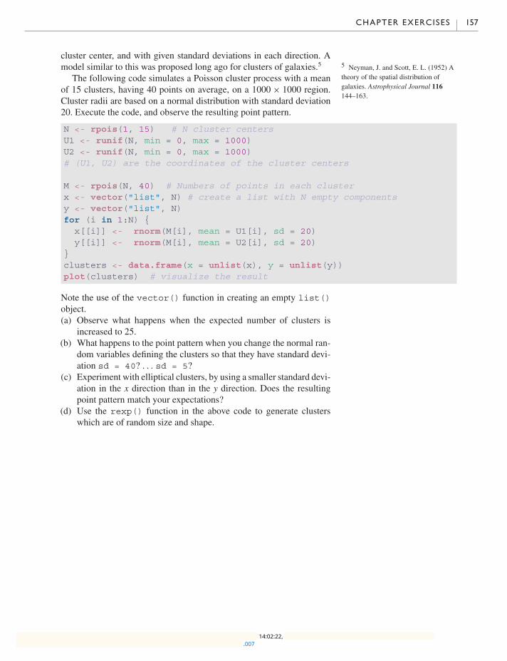
CHAPTER EXERCISES 157
cluster center, and with given standard deviations in each direction. Amodel similar to this was proposed long ago for clusters of galaxies.5 5 Neyman, J. and Scott, E. L. (1952) A
theory of the spatial distribution ofgalaxies. Astrophysical Journal 116144–163.
The following code simulates a Poisson cluster process with a meanof 15 clusters, having 40 points on average, on a 1000 × 1000 region.Cluster radii are based on a normal distribution with standard deviation20. Execute the code, and observe the resulting point pattern.
N <- rpois(1, 15) # N cluster centersU1 <- runif(N, min = 0, max = 1000)U2 <- runif(N, min = 0, max = 1000)# (U1, U2) are the coordinates of the cluster centers
M <- rpois(N, 40) # Numbers of points in each clusterx <- vector("list", N) # create a list with N empty componentsy <- vector("list", N)for (i in 1:N) {
x[[i]] <- rnorm(M[i], mean = U1[i], sd = 20)y[[i]] <- rnorm(M[i], mean = U2[i], sd = 20)
}clusters <- data.frame(x = unlist(x), y = unlist(y))plot(clusters) # visualize the result
Note the use of the vector() function in creating an empty list()object.(a) Observe what happens when the expected number of clusters is
increased to 25.(b) What happens to the point pattern when you change the normal ran-
dom variables defining the clusters so that they have standard devi-ation sd = 40? . . . sd = 5?
(c) Experiment with elliptical clusters, by using a smaller standard devi-ation in the x direction than in the y direction. Does the resultingpoint pattern match your expectations?
(d) Use the rexp() function in the above code to generate clusterswhich are of random size and shape.
.00714:02:22,
6
Computational linear algebra
Linear algebra deals with vector spaces and linear operations on them. Inmathematics, we usually represent vectors as column vectors of numbers,and linear operations as matrices. Applying a linear operation to a vectorbecomes multiplication of a column vector by a matrix, and compositionof operations is matrix multiplication.
One of the most important applications of linear algebra is in solvingsystems of linear equations. For example, we represent the system
3x1 − 4x2 = 6,
x1 + 2x2 = −3
as
Ax = b,
where
A =[3 −41 2
], x =
[x1x2
], b =
[6
−3
]and solve it as
x = A−1b =[
0.2 0.4−0.1 0.3
] [6
−3
]=
[0
−1.5
].
Linear algebra is also extensively used in statistics in linear regression,smoothing, simulation, and so on. We will touch on some of these applica-tions in this book, but most of them are beyond our scope.
From a computational point of view, many of the issues in linear alge-bra come down to solving systems of linear equations efficiently and accu-rately. In order to assess the accuracy we need to understand the propertiesof the matrices; this understanding is valuable in itself. Efficiency oftenmeans formulating problems differently than we would from a strict math-ematical point of view. For example, as we will see below, we would notnormally solve Ax = b using the mathematical solution x = A−1b: compu-tationally, this is both inefficient and inaccurate.
In this chapter, we will present several approaches to this problem,and illustrate them with R code. R incorporates routines for linear algebra
.00814:05:00,

6 .1 VECTORS AND MATRICES IN R 159
computations from the LAPACK1 library. This is a well-tested, well-trusted 1 Anderson. E., Bai, Z., Bischof, C.et al. (1999) LAPACK Users’Guide.Third Edition. SIAM. Available on-lineat www.netlib.org/lapack/lug/.
library, and R is an excellent platform for computational linear algebra.However, as with all numerical computation, understanding the underlyingtheory is essential in order to obtain reliable results.
6.1 Vectors and matrices in R
Numeric “vector” and “matrix” objects in R are a close match to mathemat-ical vectors and matrices. (R also allows other types of data in its vectorsand matrices, but that won’t concern us here.) R normally makes no distinc-tion between column vectors and row vectors, though it does allowmatriceswith one column or one row when this distinction is important.
Numeric matrices in R are printed as rectangular arrays of numbers, butare stored internally as vectors with dimension attributes. For the purposeof computational linear algebra, the internal storage can usually be ignored.
6.1.1 Constructing matrix objectsMatrices can be constructed using the functions matrix(), cbind() orrbind().
Syntaxmatrix(data, nrow, ncol) # data is a vector of nrow*ncol valuescbind(d1, d2, ..., dm) # d1, ..., dm are vectors (columns)rbind(d1, d2, ..., dn) # d1, ..., dn are vectors (rows)
Example 6.1Hilbert matrices are often studied in numerical linear algebra because theyare easy to construct but have surprising properties.
H3 <- matrix(c(1, 1/2, 1/3, 1/2, 1/3, 1/4, 1/3, 1/4, 1/5), nrow = 3)H3
## [,1] [,2] [,3]## [1,] 1.0000000 0.5000000 0.3333333## [2,] 0.5000000 0.3333333 0.2500000## [3,] 0.3333333 0.2500000 0.2000000
Here H3 is the 3 × 3 Hilbert matrix, where entry (i, j) is 1/(i+ j − 1).Note that ncol is not required in the command that created it, since thedata argument has been assigned a vector consisting of nine elements; itis clear that if there are three rows there must also be three columns.
We could also construct this matrix by binding columns together asfollows:
1/cbind(seq(1, 3), seq(2, 4), seq(3, 5))
## [,1] [,2] [,3]## [1,] 1.0000000 0.5000000 0.3333333## [2,] 0.5000000 0.3333333 0.2500000## [3,] 0.3333333 0.2500000 0.2000000
.00814:05:00,
160 COMPUTATIONAL LINEAR ALGEBRA
In this example, rbind() would give the same result, because ofsymmetry.
Matrices are not necessarily square.
Example 6.2For some simple non-square examples, consider
matrix(seq(1, 12), nrow = 3)
## [,1] [,2] [,3] [,4]## [1,] 1 4 7 10## [2,] 2 5 8 11## [3,] 3 6 9 12
and
x <- seq(1, 3)x2 <- xˆ2X <- cbind(x, x2)X
## x x2## [1,] 1 1## [2,] 2 4## [3,] 3 9
The matrix X, above, could also have been constructed as
X <- matrix(c(1, 2, 3, 1, 4, 9), ncol = 2)
though it will print differently, because we haven’t entered any columnnames.
Exercises1 Use the matrix(), seq(), and rep() functions to construct the
following 5 × 5 Hankel matrix:
A =
⎡⎢⎢⎢⎢⎣1 2 3 4 52 3 4 5 63 4 5 6 74 5 6 7 85 6 7 8 9
⎤⎥⎥⎥⎥⎦ .
Convert the code into a function which can be used to construct matricesof dimension n× n which have the same pattern. Use the function tooutput 10 × 10 and 12 × 12 Hankel matrices.
2 Use rbind() to stack the vectors [0.1 0.5 0.0 0.4], [0.2 0.3 0.5 0.0],[0.3 0.0 0.5 0.2], and [0.2 0.3 0.2 0.3] into a 4 × 4 matrix. Assign theresult to an object called P.
.00814:05:00,

6 .1 VECTORS AND MATRICES IN R 161
3 Use cbind() to construct the following 7 × 3 matrix:
W =
⎡⎢⎢⎢⎢⎢⎢⎢⎢⎣
1 2 41 3 71 4 51 5 61 6 71 7 51 8 3
⎤⎥⎥⎥⎥⎥⎥⎥⎥⎦.
6.1.2 Accessing matrix elements; row and column namesIndexing of matrix elements is the same as for data frames: the (i, j)element is located in the ith row and jth column. For example, the (3, 2)element of X is 9. We can access this element using
X[3, 2]
## x2## 9
We can access the ith row using X[i,], and the jth column usingX[, j]. For example,
X[3,]
## x x2## 3 9
X[, 2]
## [1] 1 4 9
When we do this, the result is usually a vector, with no dimension informa-tion kept. If we want to maintain the result as a row or column vector, weuse the optional drop = FALSE argument when we index:
X[3, , drop = FALSE]
## x x2## [1,] 3 9
X[, 2, drop = FALSE]
## x2## [1,] 1## [2,] 4## [3,] 9
As X shows, it is possible for the rows and/or columns of a matrix tohave individual names. For example,
colnames(X)
## [1] "x" "x2"
In this example, the rows do not have names:
rownames(X)
## NULL
.00814:05:00,
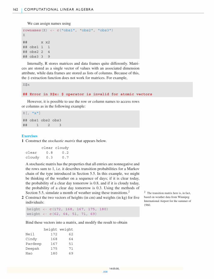
162 COMPUTATIONAL LINEAR ALGEBRA
We can assign names using
rownames(X) <- c("obs1", "obs2", "obs3")X
## x x2## obs1 1 1## obs2 2 4## obs3 3 9
Internally, R stores matrices and data frames quite differently. Matri-ces are stored as a single vector of values with an associated dimensionattribute, while data frames are stored as lists of columns. Because of this,the $ extraction function does not work for matrices. For example,
X$x
## Error in X$x: $ operator is invalid for atomic vectors
However, it is possible to use the row or column names to access rowsor columns as in the following example:
X[, "x"]
## obs1 obs2 obs3## 1 2 3
Exercises1 Construct the stochastic matrix that appears below.
clear cloudyclear 0.8 0.2cloudy 0.3 0.7
A stochastic matrix has the properties that all entries are nonnegative andthe rows sum to 1, i.e. it describes transition probabilities for a Markovchain of the type introduced in Section 5.5. In this example, we mightbe thinking of the weather on a sequence of days; if it is clear today,the probability of a clear day tomorrow is 0.8, and if it is cloudy today,the probability of a clear day tomorrow is 0.3. Using the methods ofSection 5.5, simulate a month of weather using these transitions.2 2 The transition matrix here is, in fact,
based on weather data from WinnipegInternational Airport for the summer of1960.
2 Construct the two vectors of heights (in cm) and weights (in kg) for fiveindividuals:
height <- c(172, 168, 167, 175, 180)weight <- c(62, 64, 51, 71, 69)
Bind these vectors into a matrix, and modify the result to obtain
height weightNeil 172 62Cindy 168 64Pardeep 167 51Deepak 175 71Hao 180 69
.00814:05:00,

6 .1 VECTORS AND MATRICES IN R 163
3 Refer to the previous exercise. Pardeep’s height is really 162 cm, Hao’sheight is really 181 cm and his weight is really 68 kg. Correct the matrixaccordingly.
6.1.3 Matrix propertiesThe dimension of a matrix is its number of rows and its number of columns.For example,
dim(X)
## [1] 3 2
Recall that the determinant of a 2 × 2 matrix[a bc d
]can be calculated as
ad − bc. For larger square matrices, the calculation becomes more compli-cated. It can be found in R using the det() function, as in
det(H3)
## [1] 0.000462963
The diagonal elements can be obtained using the diag() function, asin
diag(X)
## [1] 1 4
diag(H3)
## [1] 1.0000000 0.3333333 0.2000000
We can then compute the trace (the sum of the diagonal entries) using ahome-made function such as
trace <- function(data) sum(diag(data))
Applying this function to the matrices constructed in Examples 6.1and 6.2, we obtain
trace(X)
## [1] 5
trace(H3)
## [1] 1.533333
The diag() function can also be used to turn a vector into a square diago-nal matrix whose diagonal elements correspond to the entries of the givenvector. For example,
diag(diag(H3))
## [,1] [,2] [,3]## [1,] 1 0.0000000 0.0## [2,] 0 0.3333333 0.0## [3,] 0 0.0000000 0.2
.00814:05:00,

164 COMPUTATIONAL LINEAR ALGEBRA
The t() function is used to calculate the matrix transpose X�:
t(X)
## obs1 obs2 obs3## x 1 2 3## x2 1 4 9
Exercises1 Verify that det(A) = det(A�) by experimenting with several matrices A.2 A matrix A is said to be skew-symmetric if
A� = −A.
Construct a 3 × 3 skew-symmetric matrix and verify that its determinantis 0. What is the trace of your matrix?
6.1.4 Triangular matricesThe functions lower.tri() and upper.tri() can be used to obtainthe lower and upper triangular parts of matrices. The output of the func-tions is a matrix of logical elements, with TRUE representing the relevanttriangular elements. For example,
lower.tri(H3)
## [,1] [,2] [,3]## [1,] FALSE FALSE FALSE## [2,] TRUE FALSE FALSE## [3,] TRUE TRUE FALSE
We can obtain the lower triangular matrix whose non-zero elementsmatch the lower triangular elements of H3 by using
Hnew <- H3Hnew[upper.tri(H3, diag = TRUE)] <- 0 # diag = TRUE causes all
# diagonal elements to be# included
Hnew
## [,1] [,2] [,3]## [1,] 0.0000000 0.00 0## [2,] 0.5000000 0.00 0## [3,] 0.3333333 0.25 0
Exercises1 Obtain a matrix which has the same upper triangular part as H3 (includ-
ing the diagonal) but is 0 below the diagonal.2 Check the output from
Hnew[lower.tri(H3)]
Is it what you expected?
.00814:05:00,
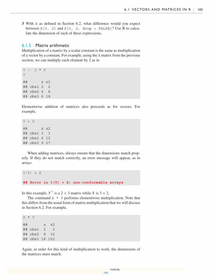
6 .1 VECTORS AND MATRICES IN R 165
3 With X as defined in Section 6.2, what difference would you expectbetween X[3, 2] and X[3, 2, drop = FALSE]? Use R to calcu-late the dimension of each of these expressions.
6.1.5 Matrix arithmeticMultiplication of a matrix by a scalar constant is the same as multiplicationof a vector by a constant. For example, using the Xmatrix from the previoussection, we can multiply each element by 2 as in
Y <- 2 * XY
## x x2## obs1 2 2## obs2 4 8## obs3 6 18
Elementwise addition of matrices also proceeds as for vectors. Forexample,
Y + X
## x x2## obs1 3 3## obs2 6 12## obs3 9 27
When adding matrices, always ensure that the dimensions match prop-erly. If they do not match correctly, an error message will appear, as inarrays
t(Y) + X
## Error in t(Y) + X: non-conformable arrays
In this example, Y� is a 2 × 3 matrix while X is 3 × 2.The command X * Y performs elementwise multiplication. Note that
this differs from the usual form ofmatrix multiplication that wewill discussin Section 6.2. For example,
X * Y
## x x2## obs1 2 2## obs2 8 32## obs3 18 162
Again, in order for this kind of multiplication to work, the dimensions ofthe matrices must match.
.00814:05:00,

166 COMPUTATIONAL LINEAR ALGEBRA
6.2 Matrix multiplication and inversion
If A and B are matrices, then the matrix product AB is the matrix represent-ing the composition of the two operations: first apply B, then apply A tothe result. For matrix multiplication to be a properly defined operation, thematrices to be multiplied must conform. That is, the number of columnsof the first matrix must match the number of rows of the second matrix.The resulting matrix AB will have its row dimension taken from A and itscolumn dimension taken from B.
In R, this form of matrix multiplication can be performed using theoperator %*%, for example
t(Y) %*% X
## x x2## x 28 72## x2 72 196
From the previous section we saw that t(Y) has three columns and X hasthree rows, so we can perform the multiplicationY�X . The result is a 2 × 2matrix, since t(Y) has two rows and X has two columns.
If we failed to transpose Y, we would obtain an error, as in
Y %*% X
## Error in Y %*% X: non-conformable arguments
The crossprod() function is a somewhat more efficient way to cal-culate Y�X :
crossprod(Y, X)
## x x2## x 28 72## x2 72 196
Note that the first argument of crossprod() is transposed automati-cally. The reason why this is more efficient than t(Y) %*% X is that thelatter needs to make a new object t(Y) before performing the multiplica-tion. If Y is a large matrix, this will consume a lot of memory and notice-able computation time. The crossprod(Y, X) function call can accessthe elements of Y directly, since the (i, j) element of Y� is simply the ( j, i)element of Y .
Exercises1 Compute 1.5X , using the matrix X that was defined at the end ofSection 6.1.1.
2 Use the crossprod() function to compute X�X and XX�. Note thedimensions of the resulting products.
.00814:05:00,

6 .2 MATRIX MULTIPL ICATION AND INVERSION 167
3 Consider the following code which compares the times for computingthe product of two matrices (A and B) and a vector v:
ABv .
A <- matrix(rep(1, 1000000), nrow = 1000) # a matrix of 1’sB <- Av <- rep(1, 1000) # a vector of 1’ssystem.time(A %*% B %*% v)
## user system elapsed## 0.906 0.005 0.916
system.time((A %*% B) %*% v)
## user system elapsed## 0.969 0.005 0.984
system.time(A %*% (B %*% v))
## user system elapsed## 0.003 0.000 0.003
(a) Is there a mathematical difference among ABv , (AB)v , and A(Bv )?(b) Explain why the third calculation takes less time than the other
calculations.(c) Can you explain the behavior that you observe upon running the
following calculations?
A <- matrix(rep(1, 1000000), nrow = 1000) # a matrix of 1’sB <- diag(1000) # 1000 x 1000 identity matrixv <- rep(1, 1000) # a vector of 1’ssystem.time(A %*% B %*% v)system.time((A %*% B) %*% v)system.time(A %*% (B %*% v))
6.2.1 Matrix inversionThe inverse of a square n× n matrix A, denoted by A−1, is the solution tothe matrix equation AA−1 = I, where I is the n× n identity matrix. We canview this as n separate systems of linear equations in n unknowns, whosesolutions are the columns of A−1. For example, with
A =[3 −41 2
]the matrix equation[
3 −41 2
] [b11 b12b21 b22
]=
[1 00 1
]is equivalent to the two equations[
3 −41 2
] [b11b21
]=
[10
]
.00814:05:00,
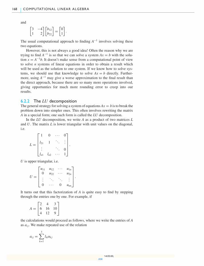
168 COMPUTATIONAL LINEAR ALGEBRA
and [3 −41 2
] [b12b22
]=
[01
].
The usual computational approach to finding A−1 involves solving thesetwo equations.
However, this is not always a good idea! Often the reason why we aretrying to find A−1 is so that we can solve a system Ax = b with the solu-tion x = A−1b. It doesn’t make sense from a computational point of viewto solve n systems of linear equations in order to obtain a result whichwill be used as the solution to one system. If we know how to solve sys-tems, we should use that knowledge to solve Ax = b directly. Further-more, using A−1 may give a worse approximation to the final result thanthe direct approach, because there are so many more operations involved,giving opportunties for much more rounding error to creep into ourresults.
6.2.2 The LU decompositionThe general strategy for solving a system of equationsAx = b is to break theproblem down into simpler ones. This often involves rewriting the matrixA in a special form; one such form is called the LU decomposition.
In the LU decomposition, we write A as a product of two matrices Land U . The matrix L is lower triangular with unit values on the diagonal,i.e.
L =
⎡⎢⎢⎢⎢⎣1 0 · · · 0
l21 1. . .
......
. . . 0ln1 ln2 · · · 1
⎤⎥⎥⎥⎥⎦ .
U is upper triangular, i.e.
U =
⎡⎢⎢⎢⎣u11 u12 · · · u1n0 u22 · · · u2n...
. . .. . .
...0 · · · 0 unn
⎤⎥⎥⎥⎦ .
It turns out that this factorization of A is quite easy to find by steppingthrough the entries one by one. For example, if
A =⎡⎣2 4 36 16 104 12 9
⎤⎦the calculations would proceed as follows, where we write the entries of Aas ai j. We make repeated use of the relation
ai j =3∑
k=1
likuk j
.00814:05:00,

6 .2 MATRIX MULTIPL ICATION AND INVERSION 169
and take advantage of knowing the 0s and 1s in L andU .
1. a11 = 2 = l11 × u11 = 1 × u11, so u11 = 2.2. a21 = 6 = l21 × u11 = l21 × 2, so l21 = 3.3. a31 = 4 = l31 × u11 = l31 × 2, so l31 = 2.4. a12 = 4 = l11 × u12, so u12 = 4.5. a22 = 16 = l21 × u12 + l22 × u22 = 3 × 4 + 1 × u22, so u22 = 4.6. a32 = 12 = l31 × u12 + l32 × u22 = 2 × 4 + l32 × 4, so l32 = 1.7. a13 = 3 = l11 × u13 = 1 × u13, so u13 = 3.8. a23 = 10 = l21 × u13 + l22 × u23 = 3 × 3 + 1 × u23, so u23 = 1.9. a33 = 9 = l31 × u13 + l32 × u23 + l33 × u33 = 2 × 3 + 1 × 1 + 1 ×
u33, so u33 = 2.
Once we have L andU in hand, solving the system of equations Ax = bis easy. We write the system as L(Ux) = b, set y = Ux, and solve Ly = bfor y first. Because L is lower triangular, this is straightforward using aprocedure known as forward substitution. Continuing the example above,with b = [−1,−2,−7]�, and setting y = [y1, y2, y3]�, we make use of therelation
bi =3∑j=1
li jy j
to calculate the following.
10. b1 = −1 = l11 × y1 = 1 × y1, so y1 = −1.11. b2 = −2 = l21 × y1 + l22 × y2 = 3 × (−1) + 1 × y2, so y2 = 1.12. b3 = −7 = l31 × y1 + l32 × y2 + l33 × y3 = 2 × (−1) + 1 × 1 +
1 × y3, so y3 = −6.
Finally, we solve Ux = y. This time the fact that U is upper triangularmeans that solving for the entries in reverse order is easy, using a procedurecalled back substitution.
13. y3 = −6 = u33 × x3 = 2 × x3, so x3 = −3.14. y2 = 1 = u22 × x2 + u23 × x3 = 4 × x2 + 1 × (−3), so x2 = 1.15. y1 = −1 = u11 × x1 + u12 × x2 + u13 × x3 = 2 × x1 + 4 × 1 + 3 ×
(−3), so x1 = 2.
By processing these steps successively, the problem of solving Ax =b has been reduced to solving 15 successive linear equations, each withjust one unknown. The procedure is easily automated. In fact, the defaultmethod used in R for solving linear equations is based on this technique; theonly substantial difference is that the ordering of the columns is rearrangedbefore factoring so that rounding error is minimized.
6.2.3 Matrix inversion in RIn R, matrices are inverted and linear systems of equations are solved usingthe solve() or qr.solve() functions. solve() uses a method basedon the LU decomposition; qr.solve() is based on theQR decompositionthat is described in Section 6.4.3.
.00814:05:00,
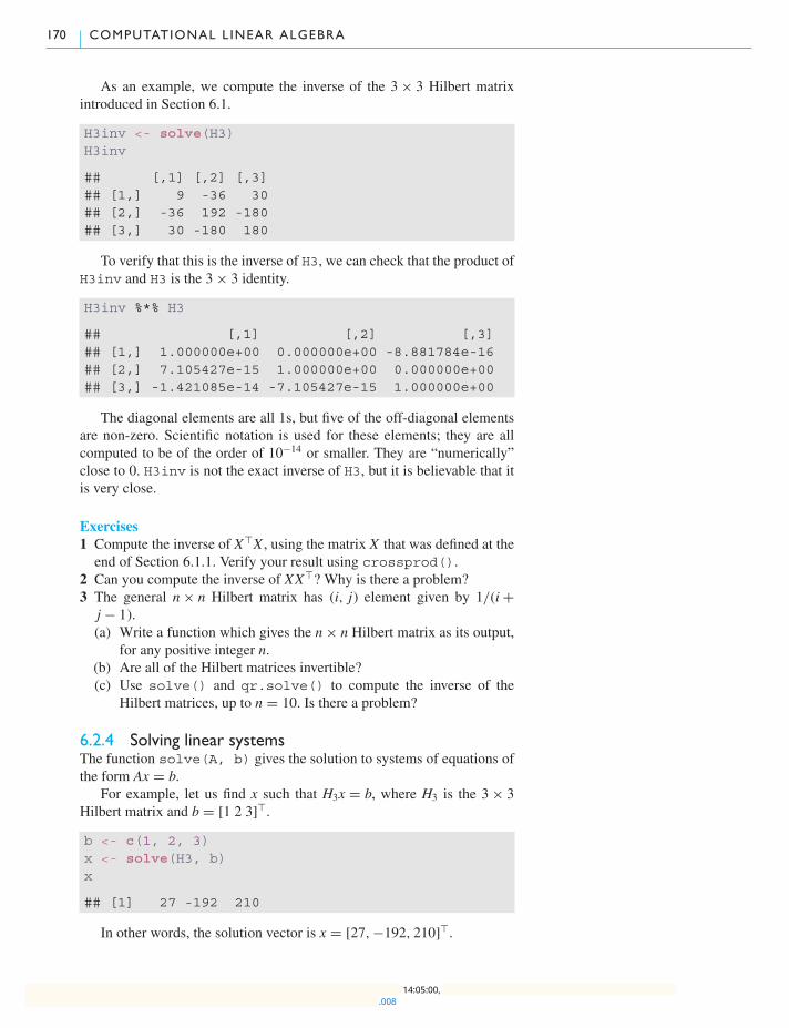
170 COMPUTATIONAL LINEAR ALGEBRA
As an example, we compute the inverse of the 3 × 3 Hilbert matrixintroduced in Section 6.1.
H3inv <- solve(H3)H3inv
## [,1] [,2] [,3]## [1,] 9 -36 30## [2,] -36 192 -180## [3,] 30 -180 180
To verify that this is the inverse of H3, we can check that the product ofH3inv and H3 is the 3 × 3 identity.
H3inv %*% H3
## [,1] [,2] [,3]## [1,] 1.000000e+00 0.000000e+00 -8.881784e-16## [2,] 7.105427e-15 1.000000e+00 0.000000e+00## [3,] -1.421085e-14 -7.105427e-15 1.000000e+00
The diagonal elements are all 1s, but five of the off-diagonal elementsare non-zero. Scientific notation is used for these elements; they are allcomputed to be of the order of 10−14 or smaller. They are “numerically”close to 0. H3inv is not the exact inverse of H3, but it is believable that itis very close.
Exercises1 Compute the inverse of X�X , using the matrix X that was defined at theend of Section 6.1.1. Verify your result using crossprod().
2 Can you compute the inverse of XX�? Why is there a problem?3 The general n× n Hilbert matrix has (i, j) element given by 1/(i+j − 1).(a) Write a function which gives the n× n Hilbert matrix as its output,
for any positive integer n.(b) Are all of the Hilbert matrices invertible?(c) Use solve() and qr.solve() to compute the inverse of the
Hilbert matrices, up to n = 10. Is there a problem?
6.2.4 Solving linear systemsThe function solve(A, b) gives the solution to systems of equations ofthe form Ax = b.
For example, let us find x such that H3x = b, where H3 is the 3 × 3Hilbert matrix and b = [1 2 3]�.
b <- c(1, 2, 3)x <- solve(H3, b)x
## [1] 27 -192 210
In other words, the solution vector is x = [27,−192, 210]�.
.00814:05:00,
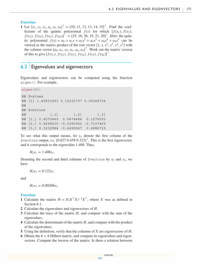
6 .3 E IGENVALUES AND EIGENVECTORS 171
Exercises1 Let [x1, x2, x3, x4, x5, x6]� = [10, 11, 12, 13, 14, 15]�. Find the coef-
ficients of the quintic polynomial f (x) for which [ f (x1), f (x2),f (x3), f (x4), f (x5), f (x6)]� = [25, 16, 26, 19, 21, 20]�. Hint: the quin-tic polynomial f (x) = a0 + a1x+ a2x2 + a3x3 + a4x4 + a5x5 can beviewed as the matrix product of the row vector [1, x, x2, x3, x4, x5] withthe column vector [a0, a1, a2, a3, a4, a5]�. Work out the matrix versionof this to give [ f (x1), f (x2), f (x3), f (x4), f (x5), f (x6)]�.
6.3 Eigenvalues and eigenvectors
Eigenvalues and eigenvectors can be computed using the functioneigen(). For example,
eigen(H3)
## $values## [1] 1.40831893 0.12232707 0.00268734#### $vectors## [,1] [,2] [,3]## [1,] 0.8270449 0.5474484 0.1276593## [2,] 0.4598639 -0.5282902 -0.7137469## [3,] 0.3232984 -0.6490067 0.6886715
To see what this output means, let x1 denote the first column of the$vectors output, i.e. [0.827 0.459 0.323]�. This is the first eigenvector,and it corresponds to the eigenvalue 1.408. Thus,
H3x1 = 1.408x1.
Denoting the second and third columns of $vectors by x2 and x3, wehave
H3x2 = 0.122x2
and
H3x3 = 0.00268x3.
Exercises1 Calculate the matrix H = X (X�X )−1X�, where X was as defined in
Section 6.1.2 Calculate the eigenvalues and eigenvectors of H.3 Calculate the trace of the matrix H, and compare with the sum of theeigenvalues.
4 Calculate the determinant of the matrixH, and compare with the productof the eigenvalues.
5 Using the definition, verify that the columns of X are eigenvectors of H.6 Obtain the 6 × 6 Hilbert matrix, and compute its eigenvalues and eigen-vectors. Compute the inverse of the matrix. Is there a relation between
.00814:05:00,
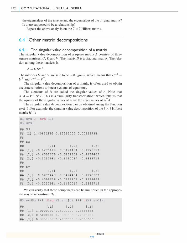
172 COMPUTATIONAL LINEAR ALGEBRA
the eigenvalues of the inverse and the eigenvalues of the original matrix?Is there supposed to be a relationship?
Repeat the above analysis on the 7 × 7 Hilbert matrix.
6.4 Other matrix decompositions
6.4.1 The singular value decomposition of a matrixThe singular value decomposition of a square matrix A consists of threesquare matrices,U , D and V . The matrix D is a diagonal matrix. The rela-tion among these matrices is
A = UDV�.
The matricesU and V are said to be orthogonal, which means thatU−1 =U� and V−1 = V�.
The singular value decomposition of a matrix is often used to obtainaccurate solutions to linear systems of equations.
The elements of D are called the singular values of A. Note thatA�A = V−1D2V . This is a “similarity transformation” which tells us thatthe squares of the singular values of A are the eigenvalues of A�A.
The singular value decomposition can be obtained using the functionsvd(). For example, the singular value decomposition of the 3 × 3 Hilbertmatrix H3 is
H3.svd <- svd(H3)H3.svd
## $d## [1] 1.40831893 0.12232707 0.00268734#### $u## [,1] [,2] [,3]## [1,] -0.8270449 0.5474484 0.1276593## [2,] -0.4598639 -0.5282902 -0.7137469## [3,] -0.3232984 -0.6490067 0.6886715#### $v## [,1] [,2] [,3]## [1,] -0.8270449 0.5474484 0.1276593## [2,] -0.4598639 -0.5282902 -0.7137469## [3,] -0.3232984 -0.6490067 0.6886715
We can verify that these components can be multiplied in the appropri-ate way to reconstruct H3.
H3.svd$u %*% diag(H3.svd$d) %*% t(H3.svd$v)
## [,1] [,2] [,3]## [1,] 1.0000000 0.5000000 0.3333333## [2,] 0.5000000 0.3333333 0.2500000## [3,] 0.3333333 0.2500000 0.2000000
.00814:05:00,

6 .4 OTHER MATRIX DECOMPOSITIONS 173
Because of the properties of the U , V , and D matrices, the singularvalue decomposition provides a simple way to compute a matrix inverse.For example, H−1
3 = VD−1U� and can be recalculated as
H3.svd$v %*% diag(1/H3.svd$d) %*% t(H3.svd$u)
## [,1] [,2] [,3]## [1,] 9 -36 30## [2,] -36 192 -180## [3,] 30 -180 180
6.4.2 The Choleski decomposition of a positivedefinite matrixIf a matrix A is positive definite, it possesses a square root. In fact, there areusually several matrices B such that B2 = A. The Choleski decompositionis similar, but the idea is to find an upper triangular matrix U such thatU�U = A. The function chol() accomplishes this task.
For example, we can compute the Choleski decomposition of the 3 × 3Hilbert matrix.
H3.chol <- chol(H3)H3.chol # This is U, the upper triangular matrix
## [,1] [,2] [,3]## [1,] 1 0.5000000 0.3333333## [2,] 0 0.2886751 0.2886751## [3,] 0 0.0000000 0.0745356
crossprod(H3.chol, H3.chol) # Multiplying t(U) %*% U to recover H3
## [,1] [,2] [,3]## [1,] 1.0000000 0.5000000 0.3333333## [2,] 0.5000000 0.3333333 0.2500000## [3,] 0.3333333 0.2500000 0.2000000
Once the Choleski decomposition of a matrix A = U�U has beenobtained, we can compute the inverse of A using the fact that A−1 =U−1U−� (where U−� is a short way to write the transpose of U−1). Thiscomputation ismuchmore stable than direct calculation ofA−1 byGaussianelimination. The function chol2inv() does this calculation. For exam-ple, we can compute the inverse of H3 as
chol2inv(H3.chol)
## [,1] [,2] [,3]## [1,] 9 -36 30## [2,] -36 192 -180## [3,] 30 -180 180
Once the Choleski decomposition has been obtained, we can computesolutions to linear systems of the form
Ax = b.
.00814:05:00,

174 COMPUTATIONAL LINEAR ALGEBRA
If A = U�U , then we see that Ux = U−�b. Therefore, the solution x canbe obtained in a two-step procedure.
1. SolveU�y = b for y. The solution will satisfy y = U−�b.2. SolveUx = y.
The first system is lower triangular, so forward substitution can be used tosolve it. The function forwardsolve() can be used for this.
The second system is upper triangular, so back substitution using thefunction backsolve() can be used.
For the problem H3x = b, where b = [1 2 3]�, we can proceed asfollows:
b <- seq(1, 3)y <- forwardsolve(t(H3.chol), b)backsolve(H3.chol, y) # the solution x
## [1] 27 -192 210
6.4.3 The QR decomposition of a matrixAnother way of decomposing a matrix A is via the QR decomposition
A = QR,
where Q is an orthogonal matrix, and R is an upper triangular matrix.This decomposition can be applied even if A is not square. Again, thisdecomposition can be used to obtain accurate solutions to linear systems ofequations.
For example, suppose we want to solve
Ax = b
for x, given the n× n matrix A and n-vector b. If we compute the QRdecomposition of A first, we can write
QRx = b.
Multiplying through by Q� on the left gives
Rx = Q�b.
This is an easier system to solve, because R is an upper triangular matrix.Note that Q�b is an easily calculated n-vector.
To obtain the decomposition, we use the qr() function. For example,
H3.qr <- qr(H3)H3.qr
## $qr## [,1] [,2] [,3]## [1,] -1.1666667 -0.6428571 -0.450000000## [2,] 0.4285714 -0.1017143 -0.105337032## [3,] 0.2857143 0.7292564 0.003901372#### $rank## [1] 3
.00814:05:00,
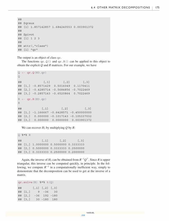
6 .4 OTHER MATRIX DECOMPOSITIONS 175
#### $qraux## [1] 1.857142857 1.684240553 0.003901372#### $pivot## [1] 1 2 3#### attr(,"class")## [1] "qr"
The output is an object of class qr.The functions qr.Q() and qr.R() can be applied to this object to
obtain the explicit Q and R matrices. For our example, we have
Q <- qr.Q(H3.qr)Q
## [,1] [,2] [,3]## [1,] -0.8571429 0.5016049 0.1170411## [2,] -0.4285714 -0.5684856 -0.7022469## [3,] -0.2857143 -0.6520864 0.7022469
R <- qr.R(H3.qr)R
## [,1] [,2] [,3]## [1,] -1.166667 -0.6428571 -0.450000000## [2,] 0.000000 -0.1017143 -0.105337032## [3,] 0.000000 0.0000000 0.003901372
We can recover H3 by multiplying Q by R:
Q %*% R
## [,1] [,2] [,3]## [1,] 1.0000000 0.5000000 0.3333333## [2,] 0.5000000 0.3333333 0.2500000## [3,] 0.3333333 0.2500000 0.2000000
Again, the inverse of H3 can be obtained from R−1Q�. Since R is uppertriangular, this inverse can be computed quickly, in principle. In the fol-lowing, we compute R−1 in a computationally inefficient way, simply todemonstrate that the decomposition can be used to get at the inverse of amatrix.
qr.solve(R) %*% t(Q)
## [,1] [,2] [,3]## [1,] 9 -36 30## [2,] -36 192 -180## [3,] 30 -180 180
.00814:05:00,
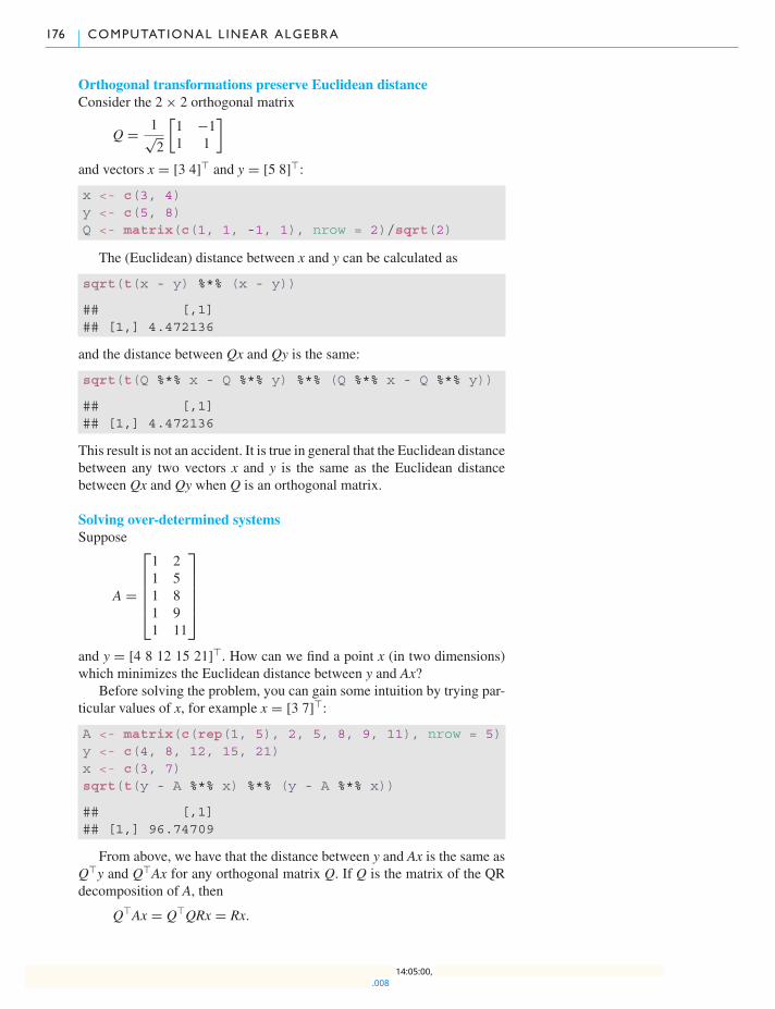
176 COMPUTATIONAL LINEAR ALGEBRA
Orthogonal transformations preserve Euclidean distanceConsider the 2 × 2 orthogonal matrix
Q = 1√2
[1 −11 1
]and vectors x = [3 4]� and y = [5 8]�:
x <- c(3, 4)y <- c(5, 8)Q <- matrix(c(1, 1, -1, 1), nrow = 2)/sqrt(2)
The (Euclidean) distance between x and y can be calculated as
sqrt(t(x - y) %*% (x - y))
## [,1]## [1,] 4.472136
and the distance between Qx and Qy is the same:
sqrt(t(Q %*% x - Q %*% y) %*% (Q %*% x - Q %*% y))
## [,1]## [1,] 4.472136
This result is not an accident. It is true in general that the Euclidean distancebetween any two vectors x and y is the same as the Euclidean distancebetween Qx and Qy when Q is an orthogonal matrix.
Solving over-determined systemsSuppose
A =
⎡⎢⎢⎢⎢⎣1 21 51 81 91 11
⎤⎥⎥⎥⎥⎦and y = [4 8 12 15 21]�. How can we find a point x (in two dimensions)which minimizes the Euclidean distance between y and Ax?
Before solving the problem, you can gain some intuition by trying par-ticular values of x, for example x = [3 7]�:
A <- matrix(c(rep(1, 5), 2, 5, 8, 9, 11), nrow = 5)y <- c(4, 8, 12, 15, 21)x <- c(3, 7)sqrt(t(y - A %*% x) %*% (y - A %*% x))
## [,1]## [1,] 96.74709
From above, we have that the distance between y and Ax is the same asQ�y and Q�Ax for any orthogonal matrix Q. If Q is the matrix of the QRdecomposition of A, then
Q�Ax = Q�QRx = Rx.
.00814:05:00,
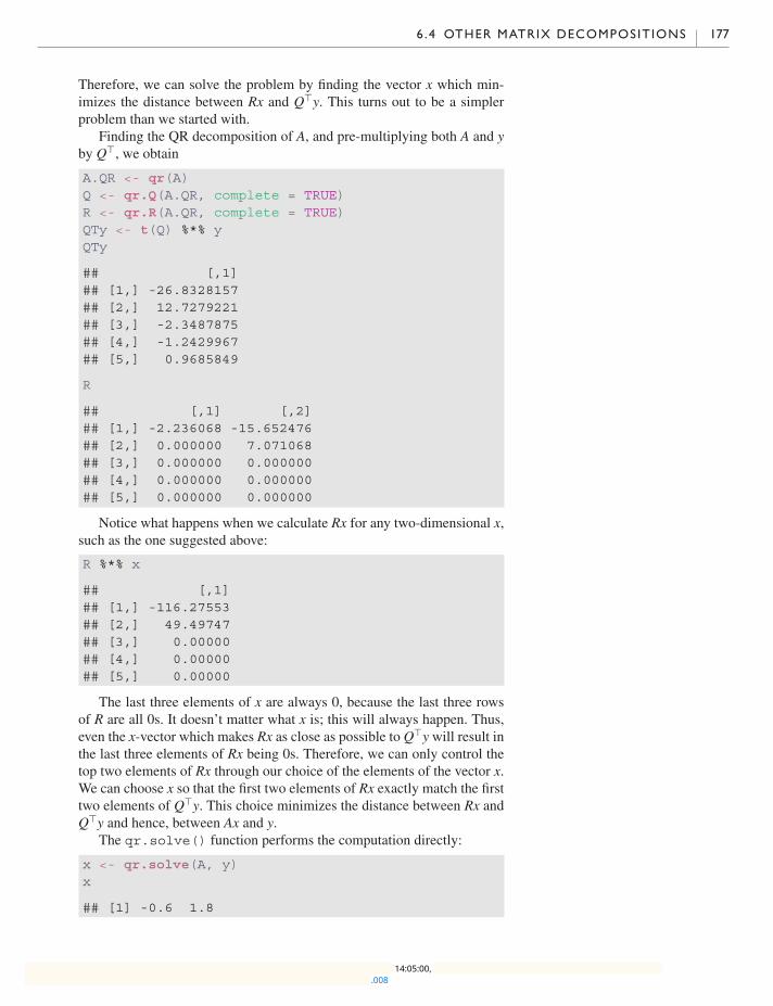
6 .4 OTHER MATRIX DECOMPOSITIONS 177
Therefore, we can solve the problem by finding the vector x which min-imizes the distance between Rx and Q�y. This turns out to be a simplerproblem than we started with.
Finding the QR decomposition of A, and pre-multiplying both A and yby Q�, we obtain
A.QR <- qr(A)Q <- qr.Q(A.QR, complete = TRUE)R <- qr.R(A.QR, complete = TRUE)QTy <- t(Q) %*% yQTy
## [,1]## [1,] -26.8328157## [2,] 12.7279221## [3,] -2.3487875## [4,] -1.2429967## [5,] 0.9685849
R
## [,1] [,2]## [1,] -2.236068 -15.652476## [2,] 0.000000 7.071068## [3,] 0.000000 0.000000## [4,] 0.000000 0.000000## [5,] 0.000000 0.000000
Notice what happens when we calculate Rx for any two-dimensional x,such as the one suggested above:
R %*% x
## [,1]## [1,] -116.27553## [2,] 49.49747## [3,] 0.00000## [4,] 0.00000## [5,] 0.00000
The last three elements of x are always 0, because the last three rowsof R are all 0s. It doesn’t matter what x is; this will always happen. Thus,even the x-vector which makes Rx as close as possible to Q�y will result inthe last three elements of Rx being 0s. Therefore, we can only control thetop two elements of Rx through our choice of the elements of the vector x.We can choose x so that the first two elements of Rx exactly match the firsttwo elements of Q�y. This choice minimizes the distance between Rx andQ�y and hence, between Ax and y.
The qr.solve() function performs the computation directly:
x <- qr.solve(A, y)x
## [1] -0.6 1.8
.00814:05:00,
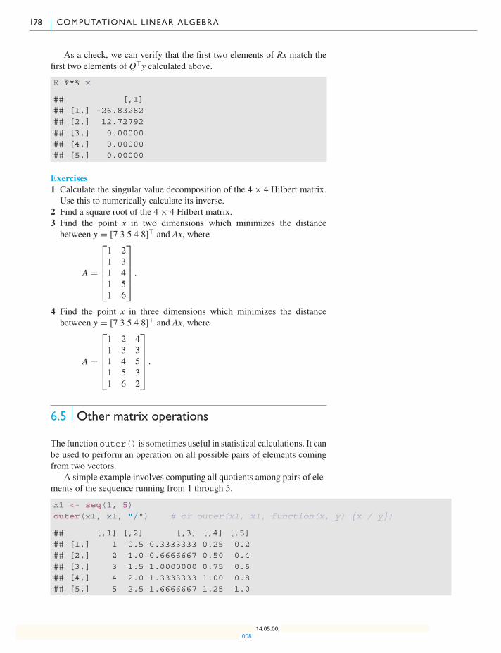
178 COMPUTATIONAL LINEAR ALGEBRA
As a check, we can verify that the first two elements of Rx match thefirst two elements of Q�y calculated above.
R %*% x
## [,1]## [1,] -26.83282## [2,] 12.72792## [3,] 0.00000## [4,] 0.00000## [5,] 0.00000
Exercises1 Calculate the singular value decomposition of the 4 × 4 Hilbert matrix.Use this to numerically calculate its inverse.
2 Find a square root of the 4 × 4 Hilbert matrix.3 Find the point x in two dimensions which minimizes the distancebetween y = [7 3 5 4 8]� and Ax, where
A =
⎡⎢⎢⎢⎢⎣1 21 31 41 51 6
⎤⎥⎥⎥⎥⎦ .
4 Find the point x in three dimensions which minimizes the distancebetween y = [7 3 5 4 8]� and Ax, where
A =
⎡⎢⎢⎢⎢⎣1 2 41 3 31 4 51 5 31 6 2
⎤⎥⎥⎥⎥⎦ .
6.5 Other matrix operations
The function outer() is sometimes useful in statistical calculations. It canbe used to perform an operation on all possible pairs of elements comingfrom two vectors.
A simple example involves computing all quotients among pairs of ele-ments of the sequence running from 1 through 5.
x1 <- seq(1, 5)outer(x1, x1, "/") # or outer(x1, x1, function(x, y) {x / y})
## [,1] [,2] [,3] [,4] [,5]## [1,] 1 0.5 0.3333333 0.25 0.2## [2,] 2 1.0 0.6666667 0.50 0.4## [3,] 3 1.5 1.0000000 0.75 0.6## [4,] 4 2.0 1.3333333 1.00 0.8## [5,] 5 2.5 1.6666667 1.25 1.0
.00814:05:00,
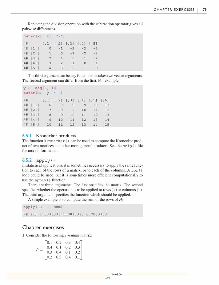
CHAPTER EXERCISES 179
Replacing the division operation with the subtraction operator gives allpairwise differences.
outer(x1, x1, "-")
## [,1] [,2] [,3] [,4] [,5]## [1,] 0 -1 -2 -3 -4## [2,] 1 0 -1 -2 -3## [3,] 2 1 0 -1 -2## [4,] 3 2 1 0 -1## [5,] 4 3 2 1 0
The third argument can be any function that takes two vector arguments.The second argument can differ from the first. For example,
y <- seq(5, 10)outer(x1, y, "+")
## [,1] [,2] [,3] [,4] [,5] [,6]## [1,] 6 7 8 9 10 11## [2,] 7 8 9 10 11 12## [3,] 8 9 10 11 12 13## [4,] 9 10 11 12 13 14## [5,] 10 11 12 13 14 15
6.5.1 Kronecker productsThe function kronecker() can be used to compute the Kronecker prod-uct of two matrices and other more general products. See the help() filefor more information.
6.5.2 apply()In statistical applications, it is sometimes necessary to apply the same func-tion to each of the rows of a matrix, or to each of the columns. A for()loop could be used, but it is sometimes more efficient computationally touse the apply() function.
There are three arguments. The first specifies the matrix. The secondspecifies whether the operation is to be applied to rows (1) or columns (2).The third argument specifies the function which should be applied.
A simple example is to compute the sum of the rows of H3.
apply(H3, 1, sum)
## [1] 1.8333333 1.0833333 0.7833333
Chapter exercises1 Consider the following circulant matrix:
P =
⎡⎢⎢⎣0.1 0.2 0.3 0.40.4 0.1 0.2 0.30.3 0.4 0.1 0.20.2 0.3 0.4 0.1
⎤⎥⎥⎦ .
.00814:05:00,
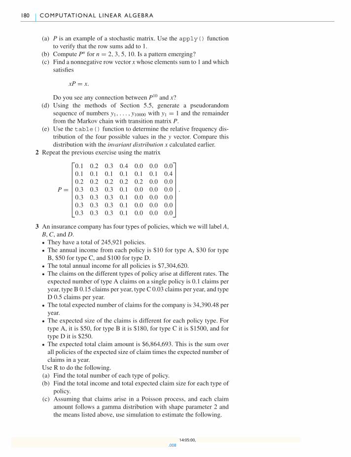
180 COMPUTATIONAL LINEAR ALGEBRA
(a) P is an example of a stochastic matrix. Use the apply() functionto verify that the row sums add to 1.
(b) Compute Pn for n = 2, 3, 5, 10. Is a pattern emerging?(c) Find a nonnegative row vector xwhose elements sum to 1 and which
satisfies
xP = x.
Do you see any connection between P10 and x?(d) Using the methods of Section 5.5, generate a pseudorandom
sequence of numbers y1, . . . , y10000 with y1 = 1 and the remainderfrom the Markov chain with transition matrix P.
(e) Use the table() function to determine the relative frequency dis-tribution of the four possible values in the y vector. Compare thisdistribution with the invariant distribution x calculated earlier.
2 Repeat the previous exercise using the matrix
P =
⎡⎢⎢⎢⎢⎢⎢⎢⎢⎣
0.1 0.2 0.3 0.4 0.0 0.0 0.00.1 0.1 0.1 0.1 0.1 0.1 0.40.2 0.2 0.2 0.2 0.2 0.0 0.00.3 0.3 0.3 0.1 0.0 0.0 0.00.3 0.3 0.3 0.1 0.0 0.0 0.00.3 0.3 0.3 0.1 0.0 0.0 0.00.3 0.3 0.3 0.1 0.0 0.0 0.0
⎤⎥⎥⎥⎥⎥⎥⎥⎥⎦.
3 An insurance company has four types of policies, which we will label A,B,C, and D.� They have a total of 245,921 policies.� The annual income from each policy is $10 for type A, $30 for typeB, $50 for type C, and $100 for type D.
� The total annual income for all policies is $7,304,620.� The claims on the different types of policy arise at different rates. Theexpected number of type A claims on a single policy is 0.1 claims peryear, type B 0.15 claims per year, type C 0.03 claims per year, and typeD 0.5 claims per year.
� The total expected number of claims for the company is 34,390.48 peryear.
� The expected size of the claims is different for each policy type. Fortype A, it is $50, for type B it is $180, for type C it is $1500, and fortype D it is $250.
� The expected total claim amount is $6,864,693. This is the sum overall policies of the expected size of claim times the expected number ofclaims in a year.
Use R to do the following.(a) Find the total number of each type of policy.(b) Find the total income and total expected claim size for each type of
policy.(c) Assuming that claims arise in a Poisson process, and each claim
amount follows a gamma distribution with shape parameter 2 andthe means listed above, use simulation to estimate the following.
.00814:05:00,

CHAPTER EXERCISES 181
(i) The variance in the total claim amount.(ii) The probability that the total claim amount will exceed the total
annual income from these policies.Write a function to do these calculations, and do it once for the over-all company income and claims, and once for each of the four typesof policy.
4 The function kappa() can be used to compute the condition numberof a given matrix (the ratio of the largest to smallest non-zero singularvalues). This gives an idea as to how bad certain numerical calculationswill be when applied to the matrix. Large values of the condition numberindicate poor numerical properties; in particular, accuracy in the numer-ical calculation of the inverse of a matrix with a large condition numberwill be poor. Calculate the respective condition numbers for the 3 × 3,5 × 5, and 7 × 7 Hilbert matrices. Interpret the results.
.00814:05:00,
7
Numerical optimization
In many areas of statistics and applied mathematics one has to solve thefollowing problem: given a function f (·), which value of x makes f (x) aslarge or as small as possible?
For example, in financial modeling f (x) might be the expected returnfrom a portfolio, with x being a vector holding the amounts invested in eachof a number of possible securities. There might be constraints on x (e.g. theamount to invest must be positive, the total amount invested must be fixed,etc.).
In statistical modeling, we may want to find a set of parameters for amodel which minimize the expected prediction errors for the model. Herex would be the parameters and f (·) would be a measure of the predictionerror.
Knowing how to do minimization is sufficient. If we want to maximizef (x), we simply change the sign and minimize − f (x). We call both opera-tions “numerical optimization.” Use of derivatives and simple algebra oftenlead to the solution of such problems, but not nearly always. Because of thewide range of possibilities for functions f (·) and parameters x, this is a richarea of computing.
7.1 The golden section search method
The golden section search method is a simple way of finding the minimizerof a single-variable function which has a single minimum on the interval[a, b].
Consider minimizing the function
f (x) = |x− 3.5| + (x− 2)2
on the interval [0, 5]. This function is not differentiable at x = 3.5, so somecare must be taken to find the minimizer. We can write an R function toevaluate f (x) as follows:
f <- function(x) {abs(x - 3.5) + (x - 2)ˆ2
}
.009 14:07:49,

7 .1 THE GOLDEN SECTION SEARCH METHOD 183
1 2 3 4 5
24
68
10
x
f(x)
Fig. 7.1 The functionf (x) = |x− 3.5| + (x− 2)2.
To check that this function has a single minimum in the interval we usethe curve() function to plot it:
curve(f, from = 1, to = 5)
The curve is displayed in Figure 7.1, where we can see that the minimizeris located near x = 2.5.
The golden section search method is an iterative method, which may beoutlined as follows.
1. Start with the interval [a, b], known to contain the minimizer.2. Repeatedly shrink it, finding smaller and smaller intervals [a′, b′] which
still contain the minimizer.3. Stop when b′ − a′ is small enough, i.e. when the interval length is less
than a pre-set tolerance.
When the search stops, the midpoint of the final interval will serve asa good approximation to the true minimizer, with a maximum error of(b′ − a′)/2.
The shrinkage step 2 begins by evaluating the function at two pointsx1 < x2 in the interior of the interval [a, b]. (How the points are chosenwill be described below.) Because we have assumed that there is a uniqueminimum, we know that if f (x1) > f (x2), then the minimum must lie tothe right of x1, i.e. in the interval [a′, b′] = [x1, b]. If f (x1) < f (x2), theminimum must lie in [a′, b′] = [a, x2] (see Figure 7.2). (What if the valuesare exactly equal? We will consider that case later.) Then new values ofx1, f (x1), x2, and f (x2) are computed, and the method is repeated until thetolerance criterion is satisfied.
The choice of the points between a and bmakes use of properties of thegolden ratio φ = (
√5 + 1)/2. The golden ratio (which we saw in Chapter 3
in the context of Fibonacci numbers) has a number of interesting algebraicproperties. We make use of the fact that 1/φ = φ − 1 and 1/φ2 = 1 − 1/φin the following. (Some authors call the value � = 1/φ the “silver ratio,”but we’ll stick with φ in our formulas.)
.009 14:07:49,

184 NUMERICAL OPTIMIZATION
1 2 3 4 5
02
46
810
12
x
f(x)
●
●
●
●
●
a
b
x1
x2aʹ
bʹx1ʹ x2ʹ
Fig. 7.2 One iteration of thegolden section search, appliedto the test functionf (x) = |x− 3.5| + (x− 2)2.
We locate the interior points at x1 = b− (b− a)/φ and x2 = a+ (b−a)/φ. The reason for this choice is as follows. After one iteration of thesearch, it is possible that we will throw away a and replace it with a′ = x1.Then the new value to use as x1 will be
x′1 = b− (b− a′)/φ
= b− (b− x1)/φ
= b− (b− a)/φ2
= a+ (b− a)/φ
= x2,
i.e. we can re-use a point we already have, we do not need a new calculationto find it, and we don’t need a new evaluation of f (x′
1), we can re-use f (x2).Similarly, if we update to b′ = x2, then x′
2 = x1, and we can re-use thatpoint.
We put this together into the following R function.
golden <- function (f, a, b, tol = 0.0000001){
ratio <- 2 / (sqrt(5) + 1)x1 <- b - ratio * (b - a)x2 <- a + ratio * (b - a)
f1 <- f(x1)f2 <- f(x2)
while(abs(b - a) > tol) {
if (f2 > f1) {b <- x2x2 <- x1f2 <- f1
.009 14:07:49,
7 .2 NEWTON–RAPHSON 185
x1 <- b - ratio * (b - a)f1 <- f(x1)
} else {a <- x1x1 <- x2f1 <- f2x2 <- a + ratio * (b - a)f2 <- f(x2)
}}return((a + b) / 2)
}
We test and see that golden() works, at least on one function:
golden(f, 1, 5)
## [1] 2.5
Exercises1 Apply the golden section minimization technique to the followingfunctions:(a) f (x) = |x− 3.5| + |x− 2| + |x− 1|,(b) f (x) = |x− 3.2| + |x− 3.5| + |x− 2| + |x− 1|.For the second function, check the graph to see that the minimizer is notunique. Show that the minimizer found by golden() depends on theinitial interval supplied to the function.
2 For an odd number of data values x1, x2, . . . , xn, the minimizer of thefunction
f (x) =n∑i=1
|x− xi|
is the sample median of the data values. (Exercise 1.(a) is an example ofthis.) Verify this result for the data sets(a) 3, 7, 9, 12, 15 and(b) 3, 7, 9, 12, 15, 18, 21.Describe, in words, what happens when the number of observations iseven.
3 Write a function which would find the maximizer of a function using thegolden section search.
7.2 Newton–Raphson
If the function to beminimized has two continuous derivatives andwe knowhow to evaluate them, we can make use of this information to give a fasteralgorithm than the golden section search.
Wewant to find aminimizer x∗ of the function f (x) in the interval [a, b].Provided the minimizer is not at a or b, x∗ will satisfy f ′(x∗) = 0. This is
.009 14:07:49,
186 NUMERICAL OPTIMIZATION
a necessary condition for x∗ to be a minimizer of f (x), but it is not suf-ficient: we must check that x∗ actually minimizes f (x). Other solutions off ′(x∗) = 0 aremaximizers and points of inflection. One sufficient conditionto guarantee that our solution is a minimum is to check that f ′′(x∗) > 0.
Now, if we have a guess x0 at a minimizer, we use the fact thatf ′′(x) is the slope of f ′(x) and approximate f ′(x) using a Taylor seriesapproximation:
f ′(x) ≈ f ′(x0) + (x− x0) f′′(x0).
Finding a zero of the right-hand side should give us an approximate solutionto f ′(x∗) = 0.
We implement this idea as follows, using the Newton–Raphson algo-rithm to approximate a solution to f ′(x∗) = 0. Start with an initial guessx0, and compute an improved guess using the solution
x1 = x0 − f ′(x0)f ′′(x0)
.
This gives a new guess at theminimizer. Then use x1 in place of x0, to obtaina new update x2. Continue with iterations of the form
xn+1 = xn − f ′(xn)f ′′(xn)
.
This iteration stops when f ′(xn) is close enough to 0. Usually, we set atolerance ε and stop when | f ′(xn)| < ε.
It can be shown that the Newton–Raphson method is guaranteed to con-verge to a local minimizer, provided the starting value x0 is close enoughto the minimizer and enough continuous derivatives exist. As with othernumerical optimization techniques, where there are multiple minimizers,Newton–Raphson won’t necessarily find the best one. However, whenf ′′(x) > 0 everywhere, there will be only one minimizer.
In actual practice, implementation of Newton–Raphson can be tricky.We may have f ′′(xn) = 0, in which case the function looks locally like astraight line, with no solution to the Taylor series approximation to f ′(x∗) =0. In this case a simple strategy is tomove a small step in the directionwhichdecreases the function value, based only on f ′(xn).
In other cases where xn is too far from the true minimizer, the Taylorapproximation may be so inaccurate that f (xn+1) is actually larger thanf (xn). When this happens one may replace xn+1 with (xn+1 + xn)/2 (orsome other value between xn and xn+1) in the hope that a smaller step willproduce better results.
Finally, there is always the possibility that the code to calculate f ′(x)or f ′′(x) may contain bugs: it is usually worthwhile to do careful checks tomake sure this is not the case.
Example 7.1We wish to find the minimizer of f (x) = e−x + x4. By inspection, we canguess that the minimizer is somewhere to the right of zero, because e−x is
.009 14:07:49,
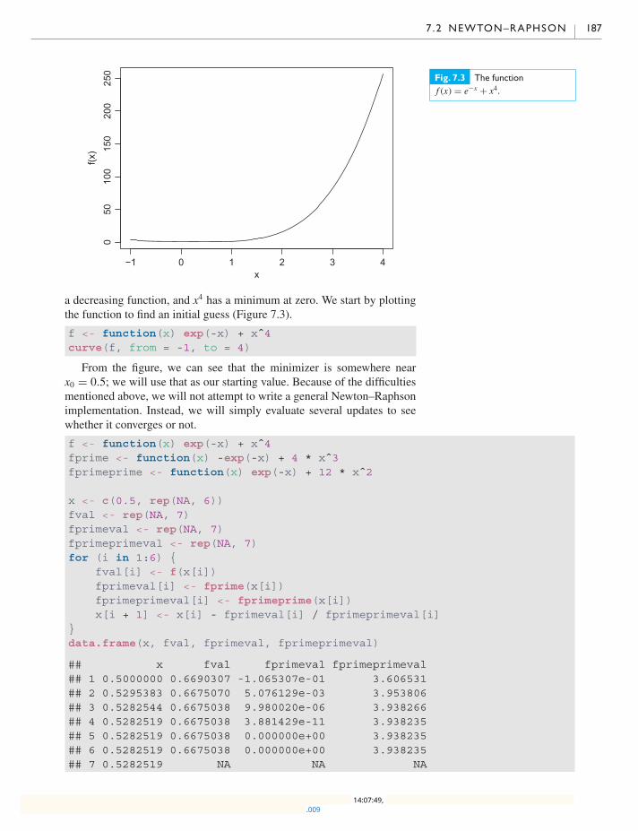
7 .2 NEWTON–RAPHSON 187
−1 0 1 2 3 4
050
100
150
200
250
x
f(x)
Fig. 7.3 The functionf (x) = e−x + x4.
a decreasing function, and x4 has a minimum at zero. We start by plottingthe function to find an initial guess (Figure 7.3).
f <- function(x) exp(-x) + xˆ4curve(f, from = -1, to = 4)
From the figure, we can see that the minimizer is somewhere nearx0 = 0.5; we will use that as our starting value. Because of the difficultiesmentioned above, we will not attempt to write a general Newton–Raphsonimplementation. Instead, we will simply evaluate several updates to seewhether it converges or not.
f <- function(x) exp(-x) + xˆ4fprime <- function(x) -exp(-x) + 4 * xˆ3fprimeprime <- function(x) exp(-x) + 12 * xˆ2
x <- c(0.5, rep(NA, 6))fval <- rep(NA, 7)fprimeval <- rep(NA, 7)fprimeprimeval <- rep(NA, 7)for (i in 1:6) {
fval[i] <- f(x[i])fprimeval[i] <- fprime(x[i])fprimeprimeval[i] <- fprimeprime(x[i])x[i + 1] <- x[i] - fprimeval[i] / fprimeprimeval[i]
}data.frame(x, fval, fprimeval, fprimeprimeval)
## x fval fprimeval fprimeprimeval## 1 0.5000000 0.6690307 -1.065307e-01 3.606531## 2 0.5295383 0.6675070 5.076129e-03 3.953806## 3 0.5282544 0.6675038 9.980020e-06 3.938266## 4 0.5282519 0.6675038 3.881429e-11 3.938235## 5 0.5282519 0.6675038 0.000000e+00 3.938235## 6 0.5282519 0.6675038 0.000000e+00 3.938235## 7 0.5282519 NA NA NA
.009 14:07:49,

188 NUMERICAL OPTIMIZATION
We see that convergence was very rapid, with the derivative numericallyequal to zero by the fourth update. The second derivative is positive there,confirming that this is a local minimum. In fact, since f ′′(x) = e−x + 12x2,the second derivative is positive everywhere, and we can be sure that thisis a global minimum.
7.3 The Nelder–Mead simplex method
In the previous sections, we have talked about two different methodsfor optimizing a function of one variable. However, when a functiondepends on multiple inputs, optimization becomes much harder. It ishard even to visualize the function once it depends on more than twoinputs.
The Nelder–Mead simplex algorithm is one method for optimizationof a function of several variables. In p dimensions, it starts with p+ 1points x1, . . . , xp+1, arranged so that when considered as vertices of ap-dimensional solid (a “simplex”), they enclose a non-zero volume. Forexample, in two dimensions the three points would not be allowed to all lieon one line so they would form a triangle, and in three dimensions the fourpoints would form a proper tetrahedron.
The points are labeled in order from smallest to largest values of f (xi),so that f (x1) ≤ f (x2) ≤ · · · ≤ f (xp+1). The idea is that to minimize f (x),we would like to drop xp+1 and replace it with a point that gives a smallervalue.We do this by calculating several proposed points zi from the existingpoints. There are four kinds of proposals, illustrated in Figure 7.4 in twodimensions. The first three refer to the midpoint of x1, . . . , xp which wecalculate as xmid = (x1 + · · · + xp)/p.
1. Reflection: reflect xp+1 through xmid to z1.2. Reflection and expansion: reflect xp+1 through xmid , and double its dis-
tance, giving z2.3. Contraction 1: contract xp+1 halfway towards xmid to give z3.4. Contraction 2: contract all points halfway towards x1, giving
z4, . . . , zp+3.
We consider each of these choices of simplex in order, based on thevalues of f (zi). It is helpful to consider the line shown in Figure 7.5 as youread through the following pseudocode outline of the decision process forone update of the simplex:
Initialization:Place the initial points in a matrix x, so that point i is inx[i,]
For i in 1:(p + 1) calculate f(x[i,])Relabel the points so thatf(x[1,]) <= f(x[2,]) <= ... <= f(x[p + 1,])
Calculate the midpoint xmid = (x[1,] + x[2,] + ... + x[p,]) / p
.009 14:07:49,
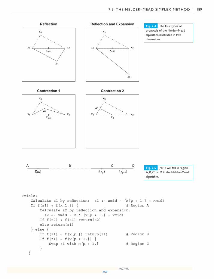
7 .3 THE NELDER–MEAD SIMPLEX METHOD 189
Reflection
x1 x2
x3
z1
xmid
Reflection and Expansion
x1 x2
x3
z2
xmid
Contraction 1
x1 x2
x3
z3
xmid
Contraction 2
x1 x2
x3
z4
z5
Fig. 7.4 The four types ofproposals of the Nelder–Meadalgorithm, illustrated in twodimensions.
f(x1) f(xp) f(xp+1)f(x1)
A B C DAFig. 7.5 f (z1) will fall in regionA, B, C, or D in the Nelder–Meadalgorithm.
Trials:Calculate z1 by reflection: z1 <- xmid - (x[p + 1,] - xmid)If f(z1) < f(x[1,]) { # Region A
Calculate z2 by reflection and expansion:z2 <- xmid - 2 * (x[p + 1,] - xmid)
If f(z2) < f(z1) return(z2)else return(z1)
} else {If f(z1) < f(x[p,]) return(z1) # Region BIf f(z1) < f(x[p + 1,]) {
Swap z1 with x[p + 1,] # Region C}
}
.009 14:07:49,

190 NUMERICAL OPTIMIZATION
1
2
2
3
3
4 5
6
7 8 9 10
0 1 2 3 4 5
01
23
45 Fig. 7.6 Contour plot of
f (x, y) = [(x− y)2 + (x− 2)2 +(y− 3)4]/10.
At this point we know f(z1) is in region D.
Try contraction 1, giving z3.If f(z3) < f(x[p + 1,]) return(z3) # Region A, B, or C
At this point nothing has worked, so we use contraction 2 to moveeverything towards x[1,]
Example 7.2In this example we try to minimize the function
f <- function(x, y) ((x - y)ˆ2 + (x - 2)ˆ2 + (y - 3)ˆ4) / 10
using the Nelder–Mead algorithm. We start by drawing a contour plot ofthe function, in order to get approximate starting values. After some experi-mentation, we obtain the plot shown in Figure 7.6 using the following code.
x <- seq(0, 5, len = 20)y <- seq(0, 5, len = 20)z <- outer(x, y, f)contour(x, y, z)
We implemented the Nelder–Mead update algorithm in an R functionwith header neldermead(x, f), where x is our matrix in the pseu-docode, and f is the function. The output of neldermead(x, f) is anupdated copy of the matrix x. The following log shows the output of nineNelder–Mead updates. Figure 7.7 shows the steps the algorithm took in thisdemonstration.
x <- matrix(c(0, 0, 2, 0, 2, 0), 3, 2)polygon(x)for (i in 1:9) {
cat(i,":")
.009 14:07:49,
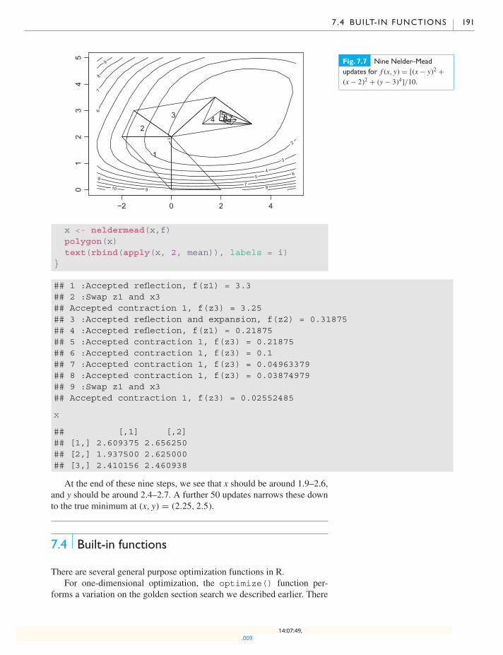
7 .4 BUILT- IN FUNCTIONS 191
1
2
3
4 5 6
6
7
7
8
8
9
9
9 10
−2 0 2 4
01
23
45
1
2
3 4 56 789
Fig. 7.7 Nine Nelder–Meadupdates for f (x, y) = [(x− y)2 +(x− 2)2 + (y− 3)4]/10.
x <- neldermead(x,f)polygon(x)text(rbind(apply(x, 2, mean)), labels = i)
}
## 1 :Accepted reflection, f(z1) = 3.3## 2 :Swap z1 and x3## Accepted contraction 1, f(z3) = 3.25## 3 :Accepted reflection and expansion, f(z2) = 0.31875## 4 :Accepted reflection, f(z1) = 0.21875## 5 :Accepted contraction 1, f(z3) = 0.21875## 6 :Accepted contraction 1, f(z3) = 0.1## 7 :Accepted contraction 1, f(z3) = 0.04963379## 8 :Accepted contraction 1, f(z3) = 0.03874979## 9 :Swap z1 and x3## Accepted contraction 1, f(z3) = 0.02552485
x
## [,1] [,2]## [1,] 2.609375 2.656250## [2,] 1.937500 2.625000## [3,] 2.410156 2.460938
At the end of these nine steps, we see that x should be around 1.9–2.6,and y should be around 2.4–2.7. A further 50 updates narrows these downto the true minimum at (x, y) = (2.25, 2.5).
7.4 Built-in functions
There are several general purpose optimization functions in R.For one-dimensional optimization, the optimize() function per-
forms a variation on the golden section search we described earlier. There
.009 14:07:49,
192 NUMERICAL OPTIMIZATION
are also multi-dimensional optimizers. The first of these is the optim()function. optim() is a general purpose wrapper for several differentoptimization methods, including Nelder–Mead, variations on Newton–Raphson, and others that we haven’t discussed.
Syntaxoptim(par, fn, ...)
The par parameter to optim() gives starting values for the param-eters. Besides telling optim() where to begin, these indicate how manyparameters will vary in its calls to fn, the second parameter. fn is an Rfunction which evaluates the function to be minimized. Its first argumentshould be a vector of the same length as par; optim() will call it repeat-edly, varying the value of this parameter, in order to find the minimum.It should return a scalar value. The optim() function has a number ofoptional parameters described on its help page. Besides those, the optionalparameters in the...list could include additional parameters to passto fn.
There are other functions in R for general function optimization: nlm()and nlminb(). In most cases optim() is preferred because it offers moreflexibility, but there may be instances where one of the others performsbetter. The constrOptim() function is aimed at cases where there arelinear inequalities expressing constraints on the parameters.
Exercises1 Use the optimize() function to minimize the following functions:
(a) f (x) = |x− 3.5| + |x− 2| + |x− 1|,(b) f (x) = |x− 3.2| + |x− 3.5| + |x− 2| + |x− 1|.
2 Use nlm() and optim() to minimize the function
f (a, b) = (a− 1) + 3.2/b+ 3 log((a)) + 3a log(b).
Note that (a) is the gamma function which can be evaluated in R usinggamma(a).
3 Re-do the previous exercise using nlminb(), noting that a and b shouldbe restricted to being nonnegative.
7.5 Linear programming
We often need to minimize (or maximize) a function subject to constraints.When the function is linear and the constraints can be expressed as lin-ear equations or inequalities, the problem is called a linear programmingproblem.
The so-called standard form for the minimization problem in linearprogramming is
minx1,x2,...,xk
C(x) = c1x1 + · · · + ckxk
.009 14:07:49,
7 .5 L INEAR PROGRAMMING 193
subject to the constraints
a11x1 + · · · + a1kxk ≥ b1,
a21x1 + · · · + a2kxk ≥ b2,
· · ·am1x1 + · · · + amkxk ≥ bm
and the nonnegativity conditions x1 ≥ 0, …, xk ≥ 0.The idea is to find values of the decision variables x1, x2, . . . , xn which
minimize the objective function C(x), subject to the constraints and non-negativity conditions.
Example 7.3A company has developed two procedures for decreasing sulfur dioxideand carbon dioxide emissions from its factory. The first procedure removesequal amounts of each gas at a per unit cost of $5. The second proce-dure removes the same amount of sulfur dioxide as the first method, butremoves twice as much carbon dioxide gas; the per unit cost of this methodis $8.
The company is required to reduce sulfur dioxide emissions by 2millionunits and carbon dioxide emissions by 3 million units. What combinationof the two emission procedures will meet this requirement at minimumcost?
Let x1 denote the amount of the first procedure to be used, and let x2denote the amount of the second procedure to be used. For convenience,we will let these amounts be expressed in millions of units.
Then the cost (in millions of dollars) can be expressed as
C = 5x1 + 8x2.
Since both methods decrease sulfur dioxide emissions at the same rate, thenumber of units of sulfur dioxide removed will then be
x1 + x2.
Noting that there is a requirement to decrease the sulfur dioxide amount by2 million units, we have the constraint
x1 + x2 ≥ 2.
The carbon dioxide reduction requirement is 3 million units, and the secondmethod removes carbon dioxide twice as fast as the first method, so we havethe second constraint
x1 + 2x2 ≥ 3.
Finally, we note that x1 and x2 must be nonnegative, since we cannot usenegative amounts of either procedure. Thus, we obtain the following linearprogramming problem:
minC = 5x1 + 8x2,
.009 14:07:49,
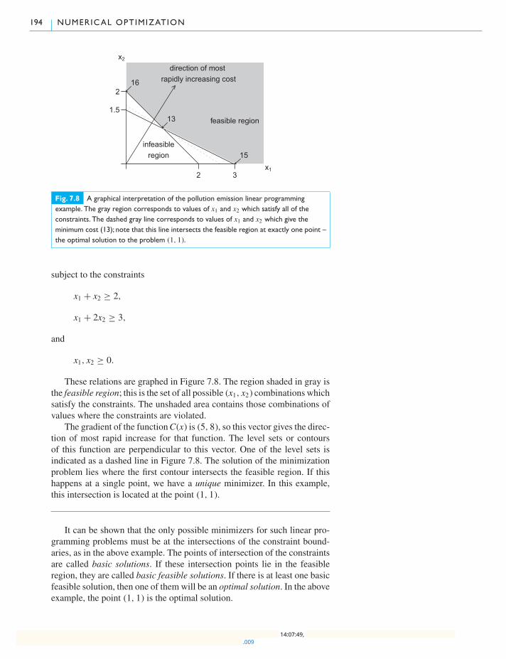
194 NUMERICAL OPTIMIZATION
2 3
1.5
2
x1
x2
16
13
15
direction of most rapidly increasing cost
feasible region
infeasibleregion
Fig. 7.8 A graphical interpretation of the pollution emission linear programmingexample. The gray region corresponds to values of x1 and x2 which satisfy all of theconstraints. The dashed gray line corresponds to values of x1 and x2 which give theminimum cost (13); note that this line intersects the feasible region at exactly one point –the optimal solution to the problem (1, 1).
subject to the constraints
x1 + x2 ≥ 2,
x1 + 2x2 ≥ 3,
and
x1, x2 ≥ 0.
These relations are graphed in Figure 7.8. The region shaded in gray isthe feasible region; this is the set of all possible (x1, x2) combinations whichsatisfy the constraints. The unshaded area contains those combinations ofvalues where the constraints are violated.
The gradient of the functionC(x) is (5, 8), so this vector gives the direc-tion of most rapid increase for that function. The level sets or contoursof this function are perpendicular to this vector. One of the level sets isindicated as a dashed line in Figure 7.8. The solution of the minimizationproblem lies where the first contour intersects the feasible region. If thishappens at a single point, we have a unique minimizer. In this example,this intersection is located at the point (1, 1).
It can be shown that the only possible minimizers for such linear pro-gramming problems must be at the intersections of the constraint bound-aries, as in the above example. The points of intersection of the constraintsare called basic solutions. If these intersection points lie in the feasibleregion, they are called basic feasible solutions. If there is at least one basicfeasible solution, then one of them will be an optimal solution. In the aboveexample, the point (1, 1) is the optimal solution.
.009 14:07:49,
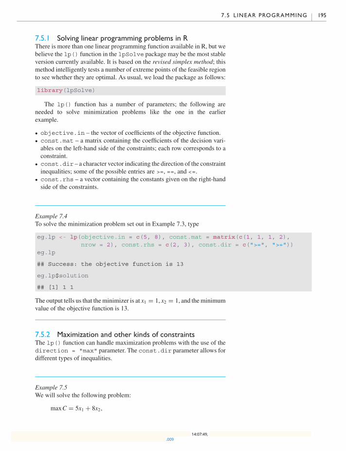
7 .5 L INEAR PROGRAMMING 195
7.5.1 Solving linear programming problems in RThere is more than one linear programming function available in R, but webelieve the lp() function in the lpSolve package may be the most stableversion currently available. It is based on the revised simplex method; thismethod intelligently tests a number of extreme points of the feasible regionto see whether they are optimal. As usual, we load the package as follows:
library(lpSolve)
The lp() function has a number of parameters; the following areneeded to solve minimization problems like the one in the earlierexample.
� objective.in – the vector of coefficients of the objective function.� const.mat – a matrix containing the coefficients of the decision vari-ables on the left-hand side of the constraints; each row corresponds to aconstraint.
� const.dir – a character vector indicating the direction of the constraintinequalities; some of the possible entries are >=, ==, and <=.
� const.rhs – a vector containing the constants given on the right-handside of the constraints.
Example 7.4To solve the minimization problem set out in Example 7.3, type
eg.lp <- lp(objective.in = c(5, 8), const.mat = matrix(c(1, 1, 1, 2),nrow = 2), const.rhs = c(2, 3), const.dir = c(">=", ">="))
eg.lp
## Success: the objective function is 13
eg.lp$solution
## [1] 1 1
The output tells us that theminimizer is at x1 = 1, x2 = 1, and theminimumvalue of the objective function is 13.
7.5.2 Maximization and other kinds of constraintsThe lp() function can handle maximization problems with the use of thedirection = "max" parameter. The const.dir parameter allows fordifferent types of inequalities.
Example 7.5We will solve the following problem:
maxC = 5x1 + 8x2,
.009 14:07:49,
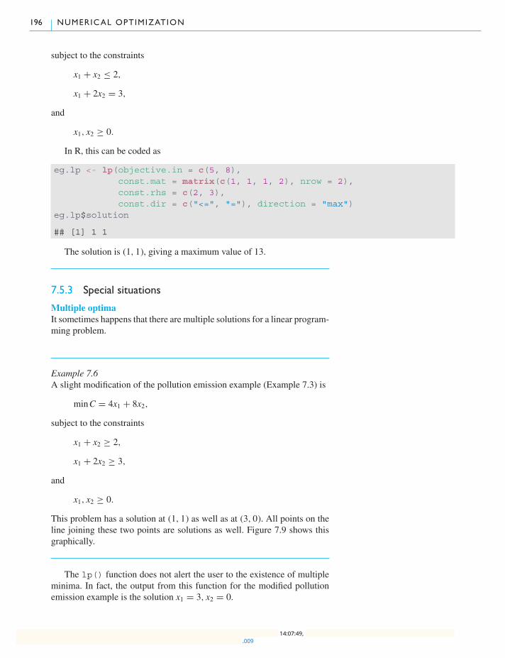
196 NUMERICAL OPTIMIZATION
subject to the constraints
x1 + x2 ≤ 2,
x1 + 2x2 = 3,
and
x1, x2 ≥ 0.
In R, this can be coded as
eg.lp <- lp(objective.in = c(5, 8),const.mat = matrix(c(1, 1, 1, 2), nrow = 2),const.rhs = c(2, 3),const.dir = c("<=", "="), direction = "max")
eg.lp$solution
## [1] 1 1
The solution is (1, 1), giving a maximum value of 13.
7.5.3 Special situations
Multiple optimaIt sometimes happens that there are multiple solutions for a linear program-ming problem.
Example 7.6A slight modification of the pollution emission example (Example 7.3) is
minC = 4x1 + 8x2,
subject to the constraints
x1 + x2 ≥ 2,
x1 + 2x2 ≥ 3,
and
x1, x2 ≥ 0.
This problem has a solution at (1, 1) as well as at (3, 0). All points on theline joining these two points are solutions as well. Figure 7.9 shows thisgraphically.
The lp() function does not alert the user to the existence of multipleminima. In fact, the output from this function for the modified pollutionemission example is the solution x1 = 3, x2 = 0.
.009 14:07:49,

7 .5 L INEAR PROGRAMMING 197
2 3
1.5
2
x1
x2
16
12
12
12
direction of most rapidly increasing cost
feasible region
infeasibleregion
Fig. 7.9 A plot of the gradient ofthe objective function and theconstraint boundaries forExample 7.6. The points on theheavy black segment are all optimalfor this problem.
DegeneracyFor a problemwithm decision variables, degeneracy arises whenmore thanm constraint boundaries intersect at a single point. This situation is quiterare, but it has potential to cause difficulties for the simplex method, so it isimportant to be aware of this condition. In very rare circumstances, degen-eracy can prevent the method from converging to the optimal solution; mostof the time, however, there is little to worry about.
Example 7.7The following problem has a point of degeneracy which is not at the opti-mum; however, thelp() function still finds the optimumwithout difficulty.
minC = 3x1 + x2,
subject to the constraints
x1 + x2 ≥ 2,
x1 + 2x2 ≥ 3,
x1 + 3x2 ≥ 4,
4x1 + x2 ≥ 4,
and
x1, x2 ≥ 0.
The constraint boundaries are plotted in Figure 7.10.This problem can be solved easily:
degen.lp <- lp(objective.in = c(3, 1),const.mat = matrix(c(1, 1, 1, 4, 1, 2, 3, 1), nrow = 4),const.rhs = c(2, 3, 4, 4), const.dir = rep(">=", 4))
degen.lp
## Success: the objective function is 3.333333
degen.lp$solution
## [1] 0.6666667 1.3333333
.009 14:07:49,
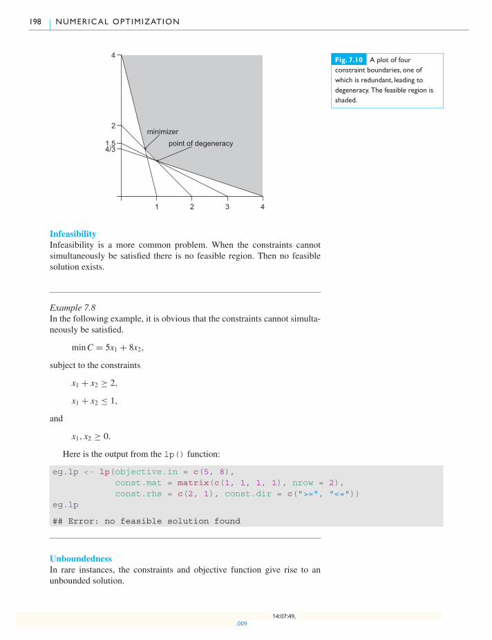
198 NUMERICAL OPTIMIZATION
1 2 3 4
4/31.5
2
4
point of degeneracyminimizer
Fig. 7.10 A plot of fourconstraint boundaries, one ofwhich is redundant, leading todegeneracy. The feasible region isshaded.
InfeasibilityInfeasibility is a more common problem. When the constraints cannotsimultaneously be satisfied there is no feasible region. Then no feasiblesolution exists.
Example 7.8In the following example, it is obvious that the constraints cannot simulta-neously be satisfied.
minC = 5x1 + 8x2,
subject to the constraints
x1 + x2 ≥ 2,
x1 + x2 ≤ 1,
and
x1, x2 ≥ 0.
Here is the output from the lp() function:
eg.lp <- lp(objective.in = c(5, 8),const.mat = matrix(c(1, 1, 1, 1), nrow = 2),const.rhs = c(2, 1), const.dir = c(">=", "<="))
eg.lp
## Error: no feasible solution found
UnboundednessIn rare instances, the constraints and objective function give rise to anunbounded solution.
.009 14:07:49,

7 .5 L INEAR PROGRAMMING 199
Example 7.9A trivial example of unboundedness arises when solving the problem
maxC = 5x1 + 8x2,
subject to the constraints
x1 + x2 ≥ 2,
x1 + 2x2 ≥ 3,
and
x1, x2 ≥ 0.
The feasible region for this problem is the same as for Example 7.3 and isplotted in Figure 7.8. However, instead of trying to minimize the objectivefunction, we are now maximizing, so we follow the direction of increasingthe objective function this time.We canmake the objective function as largeas we wish, by taking x1 and x2 arbitrarily large.
Here is what happens when lp() is applied to this problem:
eg.lp <- lp(objective.in = c(5, 8),const.mat = matrix(c(1, 1, 1, 2), nrow = 2),const.rhs = c(2, 3), const.dir = c(">=", ">="),direction = "max")
eg.lp
## Error: status 3
The condition of unboundedness will most often arise when constraintsand/or the objective function have not been formulated correctly.
7.5.4 Unrestricted variablesSometimes a decision variable is not restricted to be nonnegative. The lp()function is not set up to handle this case directly. However, a simple devicegets around this difficulty.
If x is unrestricted in sign, then x can be written as x1 − x2, where x1 ≥ 0and x2 ≥ 0. This means that every unrestricted variable in a linear pro-gramming problem can be replaced by the difference of two nonnegativevariables.
Example 7.10We will solve the following problem:
minC = x1 + 10x2,
subject to the constraints
x1 + x2 ≥ 2,
x1 − x2 ≤ 3,
.009 14:07:49,
200 NUMERICAL OPTIMIZATION
and
x1 ≥ 0.
Noting that x2 is unrestricted in sign, we set x2 = x3 − x4 for nonnega-tive x3 and x4. Plugging these new variables into the problem gives
minC = x1 + 10x3 − 10x4,
subject to the constraints
x1 + x3 − x4 ≥ 2,
x1 − x3 + x4 ≤ 3,
and
x1 ≥ 0, x3 ≥ 0, x4 ≥ 0.
Converting this to R code, we have
unres.lp <- lp(objective.in = c(1, 10, -10),const.mat = matrix(c(1, 1, 1, -1, -1, 1), nrow = 2),const.rhs = c(2, 3), const.dir = c(">=", "<="))
unres.lp
## Success: the objective function is -2.5
unres.lp$solution
## [1] 2.5 0.0 0.5
The solution is given by x1 = 2.5 and x2 = x3 − x4 = −0.5.
7.5.5 Integer programmingDecision variables are often restricted to be integers. For example, wemight want to minimize the cost of shipping a product by using one, two, orthree different trucks. It is not possible to use a fractional number of trucks,so the number of trucks must be integer-valued.
Problems involving integer-valued decision variables are called integerprogramming problems. Simple rounding of a non-integer solution to thenearest integer is not good practice; the result of such rounding can be asolution which is quite far from the optimal solution.
The lp() function has a facility to handle integer-valued variablesusing a technique called the branch and bound algorithm. The int.vecargument can be used to indicate which variables have integer values.
Example 7.11Find nonnegative x1, x2, x3, and x4 to minimize
C(x) = 2x1 + 3x2 + 4x3 − x4,
.009 14:07:49,
7 .5 L INEAR PROGRAMMING 201
subject to the constraints
x1 + 2x2 ≥ 9,
3x2 + x3 ≥ 9,
and
x2 + x4 ≤ 10.
Furthermore, x2 and x4 can take only integer values. To set up and solvethis problem in R, type
integ.lp <- lp(objective.in = c(2, 3, 4, -1),const.mat = matrix(c(1, 0, 0, 2, 3, 1, 0, 1, 0, 0, 0, 1), nrow = 3),const.dir = c(">=", ">=", "<="), const.rhs = c(9, 9, 10),int.vec = c(2, 4))
integ.lp
## Success: the objective function is 8
integ.lp$solution
## [1] 1 4 0 6
Thus, the best solution when x2 and x4 are integer-valued is x1 = 1, x2 = 4,x3 = 0, and x4 = 6.
Here is what happens when the integer variables are ignored:
wrong.lp <- lp(objective.in = c(2, 3, 4, -1),const.mat = matrix(c(1, 0, 0, 2, 3, 1, 0, 1, 0, 0, 0, 1), nrow = 3),const.dir = c(">=", ">=", "<="), const.rhs = c(9, 9, 10))
wrong.lp
## Success: the objective function is 8
wrong.lp$solution
## [1] 0.0 4.5 0.0 5.5
Rounding the solution to the nearest integer will lead to a violation ofthe first constraint (if x2 is taken to be 4) or to a minimum value of theobjective function that is larger than 8 (if x2 = 5).
7.5.6 Alternatives to lp()The lp() function provides an interface to code written in C. There isanother function in the linprog package called solveLP() which iswritten entirely in R; this latter function solves large problems much moreslowly than the lp() function, but it provides more detailed output. Wenote also the function simplex() in the boot package.
It should also be noted that, for very large problems, the simplexmethodmight not converge quickly enough; better procedures, called interior pointmethods, have been discovered recently, and are implemented in otherprogramming languages, but not yet in R.
.009 14:07:49,
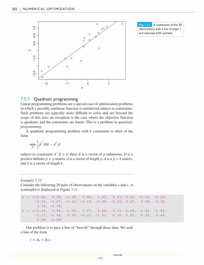
202 NUMERICAL OPTIMIZATION
●
●
●
●
●
●
●
●
●
●
●
●
●
●
●
●
●
●
●
●
−2 −1 0 1
−2.0
−1.0
0.0
0.5
1.0
x
yFig. 7.11 A scatterplot of the 20observations with a line of slope 1and intercept 0.05 overlaid.
7.5.7 Quadratic programmingLinear programming problems are a special case of optimization problemsin which a possibly nonlinear function is minimized subject to constraints.Such problems are typically more difficult to solve and are beyond thescope of this text; an exception is the case where the objective functionis quadratic and the constraints are linear. This is a problem in quadraticprogramming.
A quadratic programming problem with k constraints is often of theform
minβ
1
2β�Dβ − d�β
subject to constraints A�β ≥ b. Here β is a vector of p unknowns, D is apositive definite p× pmatrix, d is a vector of length p, A is a p× kmatrix,and b is a vector of length k.
Example 7.12Consider the following 20 pairs of observations on the variables x and y. Ascatterplot is displayed in Figure 7.11.
x <- c(0.45, 0.08, -1.08, 0.92, 1.65, 0.53, 0.52, -2.15, -2.20,-0.32, -1.87, -0.16, -0.19, -0.98, -0.20, 0.67, 0.08, 0.38,0.76, -0.78)
y <- c(1.26, 0.58, -1.00, 1.07, 1.28, -0.33, 0.68, -2.22, -1.82,-1.17, -1.54, 0.35, -0.23, -1.53, 0.16, 0.91, 0.22, 0.44,0.98, -0.98)
Our problem is to pass a line of “best-fit” through these data. We seeka line of the form
y = β0 + β1x,
.009 14:07:49,

7 .5 L INEAR PROGRAMMING 203
where β0 is the y-intercept and β1 is the slope. However, we have additionalbackground information about these data that indicate that the slope β1 ofthe required line is at least 1.
The line we want is the one that minimizes the sum of the squaredvertical distances between the observed points and the line itself:
minβ0,β1
20∑i=1
(yi − β0 − β1xi)2.
Our extra information about the slope tells us that this minimization issubject to the constraint β1 ≥ 1.
This is an example of a restricted least-squares problem and is equiva-lent to
minβ
β�X�Xβ − 2y�Xβ,
subject to
Aβ ≥ b,
where A = [0 1], β = [β0 β1]�, y is a column vector consisting of the20 y measurements, and X is a matrix consisting of two columns, wherethe first column contains only 1s and the second column contains the 20 xobservations:
X =
⎡⎢⎢⎣1 x11 x2... ...
1 xn
⎤⎥⎥⎦ =
⎡⎢⎢⎣1 0.451 0.08... ...
1 −0.78
⎤⎥⎥⎦ .
We then have
X�X =[
n∑n
i=1 xi∑ni=1 xi
∑ni=1 x
2i
]=
[20 −3.89
−3.89 21.4
]and
y�X =[
n∑i=1
yi
n∑i=1
xiyi
]= [−2.89 20.7585].
This is a quadratic programming problem with D = X�X and d = y�X .
Linear programming methods have been adapted to handle quadraticprogramming problems. The solve.QP() function is in the quadprogpackage. It solves minimization problems, and the following are the param-eters which are required:
� Dmat – a matrix containing the elements of the matrix (D) of thequadratic form in the objective function.
� dvec – a vector containing the coefficients of the decision variables inthe objective function.
� Amat – a matrix containing the coefficients of the decision variables inthe constraints; each row of the matrix corresponds to a constraint.
.009 14:07:49,
204 NUMERICAL OPTIMIZATION
� bvec – a vector containing the constants given on the right-hand side ofthe constraints.
� mvec – a number indicating the number of equality constraints. Bydefault, this is 0. If it is not 0, the equality constraints should be listedahead of the inequality constraints.
The output from this function is a list whose first two elements are thevector that minimizes the function and the minimum value of the function.
Example 7.13For the restricted least squares problem of Example 7.12, we must first setup the matricesD and A as well as the vectors b and d. Here,D = X�X andd = X�y.
library(quadprog) # load quadprog package
X <- cbind(rep(1, 20), x)XX <- t(X) %*% XXy <- t(X) %*% yA <- matrix(c(0, 1), ncol = 1)b <- 1
solve.QP(Dmat = XX, dvec = Xy, Amat = A, bvec = b)
## $solution## [1] 0.05 1.00#### $value## [1] -10.08095#### $unconstrained.solution## [1] 0.04574141 0.97810494#### $iterations## [1] 2 0#### $Lagrangian## [1] 0.4521#### $iact## [1] 1
From the output, we see that the required line is
y = 0.05 + x.
The rest of the output is indicating that the constraint is active. If the uncon-strained problem had yielded a slope larger than 1, the constraint wouldhave been inactive, and the solution to the unconstrained problem wouldbe the same as the solution to the constrained problem.
.009 14:07:49,

7 .5 L INEAR PROGRAMMING 205
Note that the decision variables in the above example were restrictedin sign. If needed, nonnegativity conditions must be explicitly set whenusing the solve.QP() function. Also, it should be noted that inequalityconstraints are all of the form >=. If your problem contains some inequalityconstraints with <=, then the constraints should be multiplied through by−1 to convert them to the required form.
It should be noted that there are more efficient ways to solve restrictedleast squares problems in other computing environments. The matrix D inthe preceding example is a diagonal matrix, and this special structure can beused to reduce the computational burden. The following example involves afull matrix. This example also places a restriction on the sign of the decisionvariables.
Example 7.14Quadratic programming can be applied to the problem of finding an optimalportfolio for an investor who is choosing how much money to invest ineach of a set of n stocks. A simple model for this problem boils down tomaximizing
x�β − k
2β�Dβ,
subject to the constraints∑n
i=1 βi = 1 and βi ≥ 0 for i = 1, . . . , n.The ith component of the β vector represents the fraction of the
investor’s fortune that should be invested in the ith stock. Note that eachelement of this vector must be nonnegative, since the investor cannot allo-cate a negative fraction of her portfolio to a stock.1 The vector x contains 1 Such behavior is called shorting a
stock, and we do not allow it here.the average daily return for each stock; the daily return value for a stockis the difference in closing price for the stock from one day to the next.Therefore, x�β represents the average daily return for the investor.
Most investors do not want to take large risks; the second term inthe objective function takes this fact into account. The factor k quantifies theinvestor’s tolerance for risk. If the investor’s goal is purely to maximize theaverage daily return without regard for the risk, then k = 0. The value of kis larger for an investor who is concerned about taking risks. The D matrixquantifies the underlying variability in the returns; it is called a covariancematrix. The diagonal elements of the D matrix are the variances of thereturns for each of the stocks. An off-diagonal element (i, j) is the covari-ance between returns of the ith and jth stocks; this is a simple measure ofrelation between the two returns.
For a specific example, we consider three stocks and set k = 2 and
D =⎡⎣0.010 0.002 0.0020.002 0.010 0.0020.002 0.002 0.010
⎤⎦ .
We assume the mean daily returns for the three stocks are 0.002, 0.005, and0.01, respectively, so x� = [0.002 0.005 0.01].
.009 14:07:49,
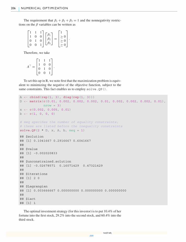
206 NUMERICAL OPTIMIZATION
The requirement that β1 + β2 + β3 = 1 and the nonnegativity restric-tions on the β variables can be written as⎡⎢⎢⎣
1 1 11 0 00 1 00 0 1
⎤⎥⎥⎦⎡⎣β1
β2
β3
⎤⎦ =
⎡⎢⎢⎣1≥ 0≥ 0≥ 0
⎤⎥⎥⎦ .
Therefore, we take
A� =
⎡⎢⎢⎣1 1 11 0 00 1 00 0 1
⎤⎥⎥⎦ .
To set this up in R, we note first that the maximization problem is equiv-alent to minimizing the negative of the objective function, subject to thesame constraints. This fact enables us to employ solve.QP().
A <- cbind(rep(1, 3), diag(rep(1, 3)))D <- matrix(c(0.01, 0.002, 0.002, 0.002, 0.01, 0.002, 0.002, 0.002, 0.01),
nrow = 3)x <- c(0.002, 0.005, 0.01)b <- c(1, 0, 0, 0)
# meq specifies the number of equality constraints;# these are listed before the inequality constraintssolve.QP(2 * D, x, A, b, meq = 1)
## $solution## [1] 0.1041667 0.2916667 0.6041667#### $value## [1] -0.002020833#### $unconstrained.solution## [1] -0.02678571 0.16071429 0.47321429#### $iterations## [1] 2 0#### $Lagrangian## [1] 0.003666667 0.000000000 0.000000000 0.000000000#### $iact## [1] 1
The optimal investment strategy (for this investor) is to put 10.4% of herfortune into the first stock, 29.2% into the second stock, and 60.4% into thethird stock.
.009 14:07:49,
CHAPTER EXERCISES 207
The optimal value of the portfolio is 0.0020 (from $value above).(Recall that the negative sign appears in the output, because we were min-imizing the negative of the objective function.)
Exercises1 (a) Find nonnegative x1, x2, x3, and x4 to minimize
C(x) = x1 + 3x2 + 4x3 + x4,
subject to the constraints
x1 − 2x2 ≥ 9,
3x2 + x3 ≥ 9,
and
x2 + x4 ≥ 10.
(b) Will the solution change if there is a requirement that any of thevariables should be integers? Explain.
(c) Suppose the objective function is changed to
C(x) = x1 − 3x2 + 4x3 + x4.
What happens to the solution now?2 Find nonnegative x1, x2, x3, and x4 to maximize
C(x) = x1 + 3x2 + 4x3 + x4,
subject to the constraints
x1 − 2x2 ≤ 9,
3x2 + x3 ≤ 9,
and
x2 + x4 ≤ 10.
Chapter exercises1 Consider the data of Example 7.12. Calculate the slope and intercept fora line of “best-fit” for these data for which the intercept is at least as largeas the slope.
2 Re-do the calculation in the portfolio allocation example using k = 1.How does being less risk-averse affect the investor’s behavior?
3 Often, there are upper bounds on the proportion that can be investedin a particular stock. Re-do the portfolio allocation problem with therequirement that no more than 50% of the investor’s fortune can be tiedup in any one stock.
4 Duncan’s Donuts Inc. (DDI) and John’s Jeans Ltd. (JJL) are two stockswith mean daily returns of 0.005 and 0.010, respectively. What is theoptimal portfolio for a completely risk-loving investor (i.e. risk tolerance
.009 14:07:49,

208 NUMERICAL OPTIMIZATION
constant k = 0)who invests only in these two stocks? (Hint: this questiondoes not require any computations.)
5 Suppose the daily returns for DDI and JJL are independent, but σ 2DDL =
0.01 and σ 2JJL = 0.04. What is the optimal allocation for an investor with
a risk tolerance constant (a) k = 1? (b) k = 2?You can use the fact that
D =[0.01 00 0.04
].
6 Repeat the preceding question under the assumption that the covariancebetween the returns for DDI and JJL is 0.01. You can use the fact that
D =[0.01 0.010.01 0.04
].
.009 14:07:49,

Appendix
Review of random variablesand distributions
When an experiment is conducted in which a number of different outcomesare possible, each outcome will have a certain probability of occurrence.
Consider a cancer treatment that will be tested on 10 patients. The num-ber of patients who show an increase in their white-blood-cell count at theend of 5 weeks of treatment cannot be predicted exactly at the beginningof the trial, so this number, which we might label N, is thought of as arandom variable. N is an example of a discrete random variable since ittakes only values from a discrete set, i.e. {0, 1, 2, . . . , 10}. The time, T ,until death could also be measured for one of the patients; again, T cannotbe predicted exactly in advance, so it is also an example of a random vari-able; since it can take a continuum of possible values, it is referred to as acontinuous random variable.
A random variable is characterized by its distribution. This specifiesthe probability that the variable will take one or more values. If X denotesthe number of heads obtained in two independent tosses of a fair coin, wemight write
P(X ≤ 1) = 0.75
to indicate that the probability of 0 or 1 head in two tosses is 0.75. In gen-eral, the function
F (x) = P(X ≤ x)
is called the distribution function of the random variable X . If F (x) has aderivative, we can define the probability density function of X as
f (x) = F ′(x).
This is often possible with continuous random variables X . Note that, inthis case,
F (y) =∫ y
−∞f (x)dx.
Among other things, note that the area under the curve specified by f (x)is 1.
.01014:09:48,

210 REVIEW OF RANDOM VARIABLES AND DISTRIBUTIONS
The expected value of a random variable is also an important concept.For continuous random variables, we can write
E[X] =∫ ∞
−∞x f (x)dx.
This is themean value of the density function f (x). It is often denoted by thesymbol μ. We also can take expectations of functions of random variablesusing the formula
E[g(X )] =∫ ∞
−∞g(x) f (x)dx.
An important example of this is the variance. The variance of a randomvariable gives an indication of the unpredictability in a random variable.Its formula is
Var(X ) = E[(X − μ)2] =∫ ∞
−∞(x− μ)2 f (x)dx.
Another important concept is that of quantile: this is the value of x forwhich F (x) takes on a particular value. When the inverse function F−1(y)is defined, the α quantile of X is given by F−1(α). For example, the 0.95quantile is the value of x for whichF (x) = 0.95; in other words, x is the 95thpercentile of the distribution. Frequently used quantiles are the median x,which satisfies F (x) = 0.5, and the upper and lower quartiles, which satisfyF (x) = 0.75 and F (x) = 0.25, respectively. When the distribution of therandom variable is discrete, F (x) will have jumps, and F−1(α) may notexist. In this case by convention we choose the smallest x with F (x) ≥ α,so quantiles always exist.
The following tables summarize properties of some commonly usedunivariate distributions; see also Tables 5.1 and 5.2.
Distribution name f (x) F (x) E[X] Var(X)
Uniform (a, b) 1/(b− a), a < x < b x (a+ b)/2 (b− a)2/12
Exponential (λ) λe−λx, x > 0 1 − e−λx 1/λ 1/λ2
Normal (μ, σ 2) [1/(σ√2π )]e−
(x−μ)2
2σ2
∫ x
−∞[1/(σ
√2π )]e−
(y−μ)2
2σ2 dy μ σ 2
Distribution name P(X = x) E[X] Var(X)
Binomial (n, p)(nx
)px(1 − p)n−x np np(1 − p)
Poisson (λ) λxe−λ/x! λ λ
We conclude this review with some brief comments about bivariate dis-tributions. In particular, suppose X and Y are continuous random variables
.01014:09:48,
REVIEW OF RANDOM VARIABLES AND DISTRIBUTIONS 211
having joint probability density f (x, y). We can define expectations usingdouble integrals:
E[g(X,Y )] =∫ ∞
−∞
∫ ∞
−∞g(x, y) f (x, y)dx dy
for functions g(x, y). In particular, setting g(X,Y ) = I(X ≤ u)I(Y ≤ v )gives
E[I(X ≤ u)I(Y ≤ v )] =∫ u
−∞
∫ v
−∞f (x, y)dx dy,
which implies that, for any u and v ,
P(X ≤ u,Y ≤ v ) =∫ u
−∞
∫ v
−∞f (x, y)dx dy.
Here, I() denotes the indicator function, which takes on the value 1 whenits argument is true, and 0 when its argument is false.
The marginal density of X is obtained by integrating over all valuesof y:
fX (x) =∫ ∞
−∞f (x, y)dy,
and similarly, the marginal density of Y is obtained by integrating over allvalues of x:
fY (y) =∫ ∞
−∞f (x, y)dx.
X and Y are stochastically independent if
f (x, y) = fX (x) fY (y).
Among other things, this implies that for independent variables P(X ≤ u,Y ≤ v ) = P(X ≤ u)P(Y ≤ v ), and by the definition of conditional proba-bility,
P(X ≤ u|Y ≤ v ) = P(X ≤ u,Y ≤ v )
P(Y ≤ v )= P(X ≤ u).
The term on the left denotes the conditional probability that X ≤ u, giventhat Y ≤ v . Intuitively, the above statement means that knowledge of thevalue ofY does not give us any additional information with which to predictthe value of X .
.01014:09:48,

Index
!, 35!=, 36.RData, 45:, 13::, 28<, 36<-, 9<=, 36=, 9==, 36>, 36>=, 36?, 28??, 30???, 31#, 8, 98%*%, 166%/%, 8%>%, 74%%, 8&, 35&&, 35ˆ, 8|, 35\n, 111||, 35
abline(), 64abs(), 88all(), 111annuity, 91any(), 85apply(), 142, 179argument list, 12arguments, 12, 92
array, 20arrows(), 64as.character(), 58as.integer(), 18attributes, 96axis(), 65
backsolve(), 174bar charts, 50barplot(), 51base, 25, 27base graphics, 49base packages, 27bias, 120binary, 22bisection algorithm, 90body, 92Boolean algebra, 34boot, 201box plot, 55box(), 65box-and-whisker plot, 55boxplot(), 56branch and bound algorithm, 200break, 89breakpoint, 111browser(), 112bugs, 107
c(), 13camel case, 99case-by-variable format, 37case-sensitive, 13cat(), 111catastrophic loss of precision, 24
cbind(), 159central limit theorem, 120chol(), 173chol2inv(), 173chron, 25, 27class(), 96column vectors, 158column-major, 20concatenation, 14, 17condition number, 181confidence interval, 121Console Pane, 5constrOptim(), 192continuous, 209contour(), 190CRAN, 4, 28crossprod(), 166
data frame, 37data.frame(), 40dates and times, 25dbinom(), 128debug(), 112debugging, 107debugonce(), 112declarative programming style, 76decomposition
Choleski, 173LU, 168QR, 174singular value, 172, 178
default value, 12det(), 163determinant, 163dexp(), 136
14:13:58,

INDEX 213
diag(), 163dim(), 39, 163dimension, 39discrete, 209distribution, 209Bernoulli, 127beta, 141binomial, 128, 141, 149, 210Cauchy, 141chi-square, 141exponential, 136, 141, 210F, 141gamma, 141geometric, 141hypergeometric, 141logistic, 141lognormal, 141negative binomial, 141normal, 120, 138, 141, 210Poisson, 132, 141, 210Student’s t, 141uniform, 121, 123, 126, 137, 141,
210Weibull, 141
distribution function, 209dnorm(), 139dot charts, 50dotchart(), 51dpois(), 132dump(), 43
edge cases, 108eigen(), 171environment, 93Eratosthenes, 84, 92example(), 29expected value, 210
factor(), 18factorial, 77FALSE, 34Fibonacci sequence, 79, 183fixed-point problem, 80floating point, 22for(), 76format(), 25, 67forwardsolve(), 174Freedman–Diaconis rule, 55function header, 92
functional programs, 76functions, 11, 91
generic functions, 96ggplot2, 49, 70global environment, 9golden ratio, 183golden section search, 182graphical parameters, 68graphics, 27grid, 49, 73, 80grid.circle(), 81grid.rect(), 73grobs, 73
help(), 28help.search(), 30help.start(), 30Hilbert matrix, 159hist(), 54histograms, 54Horner’s rule, 118
IDE, 3if(), 82imperative programming style,
76importance sampling, 153indices, 14
logical, 26, 35negative, 14zero, 15
Inf, 26install.packages(), 28integer, 24integer programming, 200integrated development environment,
3interior point methods, 201interquartile range, 56invariant distribution, 143invisible(), 96IQR, 56is.na(), 26, 109ISOdate(), 25ISOdatetime(), 25
jitter(), 135jpeg(), 68
kappa(), 181knitr, xi, 4, 27kronecker(), 179
L, 24LAPACK, 159lapply(), 42lattice, 49, 72law of large numbers, 120, 147,
148leaflet, 74legend(), 64levels(), 19library, 27Lilypond, 144linear operations, 158linear programming, 192lines(), 64linprog, 201list(), 42, 157load(), 45logical vectors, 82lower.tri(), 164lp(), 195lpSolve, 195ls(), 13
magrittr, 74Markov chain, 143, 162Markov chain Monte Carlo,
143matrix inverse, 167matrix multiplication, 158matrix(), 19, 159maximization, 182MCMC, 143mean(), 23median(), 33methods, 96microbenchmark, 116minimization, 182Monte Carlo, 120MPV, 67mtext(), 65
NA, 25namespace, 95NaN, 25ncol(), 38
14:13:58,

214 INDEX
Nelder–Mead simplex algorithm,188
Newton’s method, 87Newton–Raphson, 185next, 89nlm(), 192nlminb(), 192non-conformable, 165, 166nrow(), 38numeric(0), 15
object oriented, 76, 95objects(), 13one-pass formula, 23open source, 3optim(), 192optimize(), 191optional parameters, 16outer(), 178
p-value, 120package, 27, 95base, 27contributed, 27
panes, 5par(), 59, 68paste(), 17, 18paste0(), 18pbinom(), 128pdf(), 68pexp(), 136pie charts, 53pie(), 54plot margins, 63plot region, 63plot(), 57plot3d(), 78plotting character, 58png(), 68pnorm(), 139points(), 64Poisson process, 133, 137polygon(), 64postscript(), 68ppois(), 132precision, 22prime numbers, 84print(), 111probability density function, 209
procedural programs, 76profiling, 117pseudorandom, 121pushViewport(), 73, 81
q(), 10qbinom(), 128qexp(), 136qnorm(), 139qpois(), 132QQ plots, 60qqline(), 135qqnorm(), 135qqplot(), 60qr(), 174qr.solve(), 169quadprog, 203quadratic programming, 202quantile, 210quantile–quantile plots, 60quitting, 10
random variable, 209rbind(), 159rbinom(), 128RColorBrewer, 63read.table, 45recursion, 103recycling, 16rejection sampling, 150relational operators, 82rep(), 16repeat, 89replicate(), 97, 130repository, 28return(), 93rexp(), 137rgl, 74, 78rm(), 44rnorm(), 139rounding error, 22row-major, 20rpois(), 132Rprof(), 117RSiteSearch(), 31RStudio, xi, 3–5, 10, 14, 28, 30, 43,
74, 98, 111rstudio.com, 4runif(), 123
S3 methods, 96sample variance, 23sample(), 17, 125save.image(), 45scan(), 145scatterplot, 57scope, 94Scott rule, 55segments(), 64seq(), 16set.seed(), 124setup, 4setwd(), 13, 43short-circuit evaluation, 35silver ratio, 183simplex method, 195simplex(), 201sink(), 44solve(), 169solveLP(), 201sos, 31Source Pane, 5source(), 43sparse, 145square root, 36stats, 27stochastic matrix, 162stopifnot(), 111str(), 39strptime(), 25Sturges rule, 55subscripts, see indicessubstr(), 17substring(), 17svd(), 172symbols(), 64system.time(), 116systems of linear equations,
158
t(), 164table(), 127task views, 28text(), 64times and dates, 25title(), 65top-down design, 103traceback(), 110TRUE, 34
14:13:58,

INDEX 215
unboundedness, 199unique(), 58upper.tri(), 164
vapply(), 42var(), 23
vector spaces, 158viewport(), 73,
81viewports, 73visual perception,
62
weighted.mean,153
while(), 86with(), 39working directory, 13workspace, 9, 10
14:13:58,