Contents lists available at SciVerse ScienceDirect

Journal of Sound and Vibration

Journal of Sound and Vibration 331 (2012) 3751–3761

0022-46

http://d

n Corr

E-m

journal homepage: www.elsevier.com/locate/jsvi

A finite element method for analysis of vibration induced bymaglev trains

S.H. Ju n, Y.S. Ho, C.C. Leong

Department of Civil Engineering, National Cheng-Kung University, Tainan City, Taiwan, ROC

a r t i c l e i n f o

Article history:

Received 2 November 2011

Received in revised form

4 April 2012

Accepted 6 April 2012

Handling Editor: L.G. Thammaglev vehicles are modeled as a combination of spring-damper elements, lumped

Available online 25 April 2012

0X/$ - see front matter & 2012 Elsevier Ltd.

x.doi.org/10.1016/j.jsv.2012.04.004

esponding author. Tel.: þ886 6 2757575x63

ail address: juju@mail.ncku.edu.tw (S.H. Ju).

a b s t r a c t

This paper developed a finite element method to perform the maglev train–bridge–soil

interaction analysis with rail irregularities. An efficient proportional integral (PI)

scheme with only a simple equation is used to control the force of the maglev wheel,

which is modeled as a contact node moving along a number of target nodes. The moving

mass and rigid links. The Newmark method with the Newton–Raphson method is then

used to solve the nonlinear dynamic equation. The major advantage is that all the

proposed procedures are standard in the finite element method. The analytic solution of

maglev vehicles passing a Timoshenko beam was used to validate the current finite

element method with good agreements. Moreover, a very large-scale finite element

analysis using the proposed scheme was also tested in this paper.

& 2012 Elsevier Ltd. All rights reserved.

1. Introduction

Maglev (magnetically levitated) trains, a new rapid transport system, have attracted more attention around the worldbecause of their fast speed and low power consumption. However, the noise and vibration induced by the maglev train–guideway interaction may cause a serious environmental problem. Moreover, the earthquake and foundation settlementmay cause a severe safety problem for maglev trains moving on the guideway. Thus, to solve those problems, the dynamicbehavior of this coupled system has to be taken into account. There are many studies that consider the mechanical andelectrical aspects of maglev systems by using the finite element method, such as Bird and Lipo [1], which presented a two-dimensional complex steady-state finite-element method for calculating the lift and thrust or breaking forces createdwhen a magnetic rotor was translationally moved and rotated over a conducting sheet. In addition, Duan et al. [2]developed a novel maglev transportation platform for ultra-precision linear motion with large travel range, and designedan optimized decoupled electromagnet spatial distribution of this platform with finite-element analysis. However, fewpapers investigate maglev train–guideway coupled systems using the finite element method. Song [3] proposed a three-dimensional (3D) finite element analysis model of guideway structures considering ultra high-speed magnetic levitationtrain–bridge interaction, in which the various improved finite elements were used to model structural members. Yang andYau [4] presented an iterative interacting method for analyzing the dynamic response of a maglev train traveling on anelevated guideway supported by piers embedded in soil, and compared the solution obtained for a 2-degree-of-freedomsystem under a harmonic force with the analytical one to verify the validity of their method. There are also some studiesthat do not use the finite element method, that examine the influence of engineering factors on a maglev coupled system.

All rights reserved.

119; fax: þ886 6 2358542.

S.H. Ju et al. / Journal of Sound and Vibration 331 (2012) 3751–37613752

Cai et al. [5] studied the dynamic interactions between the maglev vehicles and flexible guideway, with an emphasis onthe effects of vehicle and guideway parameters, and the Bernoulli–Euler beam equation was used to model thecharacteristics of the guideway. Kwon et al. [6] found that the vibrations of the vehicle were significantly affected byits speed and wind forces because of the strong vehicle–bridge interaction, and that the ride quality of the maglev vehiclecould be diminished by the low frequency vibrations induced by the guideway bridge as well as by turbulent wind. Yau [7]indicated that an increase in the levitation gap for a maglev vehicle might result in a larger vehicle response, but theresponse of the maglev vehicle with a smaller air gap would be significantly amplified at higher speeds once groundsettlement occurs at the guideway supports. Yim et al. [8] predicted the curving performance with the greatest accuracypossible, in order to improve electromagnetic suspension and establish guideway design specifications. Han et al. [9]proposed a full vehicle multi-body dynamic model to facilitate rigorous ride quality prediction for an EMS-type maglevvehicle, and this could be used along with the results of earlier studies to suggest cost-effective specifications for guidewayconstruction tolerances and stiffness and the EMS. Yau [10] demonstrated a hybrid controller with the ability to adjust thelevitation gaps in a prescribed stable region for safety reasons and to reduce the vehicle’s acceleration response for ridequality when a controlled maglev train travels over a suspended guideway shaken by horizontal earthquakes. Hu et al. [11]simulated the dynamic behaviors of both vehicle and guideway to investigate how the locations of the passenger cabincenter of mass and asymmetric suspension characteristics of the vehicle suspensions influence high speed vehicle–guideway interaction.

A 3D finite element method was developed in this study to perform the maglev train–bridge–soil interaction analysiswith an efficient proportional integral (PI) scheme. The moving maglev vehicles are modeled as a combination of wheelforces, spring-damper elements, lumped mass and rigid links. The Newmark method with the Newton–Raphson method isthen used to solve the nonlinear dynamic equation. Since the proposed procedures are standard in the finite elementmethod, a general maglev train–bridge–soil interaction analysis, such as simulations with seismic loads and foundationsettlements, can be appropriately performed.

2. Control system of maglev trains

Maglev trains can be separated into two systems, depending on which type of magnetic force is used to propel them,i.e., the attractive or repulsive forces. When the former is used to levitate the vehicle, it is called an EMS (electro magneticsuspension) system, while the latter, is called an EDS (electro dynamic suspension) system. Since there is no drag for eithersystem except the air resistance, both are faster than rail-wheeled train systems, and the highest speed can be over500 km/h, thus competing with aviation. In this paper, an EMS system maglev train is examined, and the levitation isprovided by an electromagnet which is connected to the primary suspension. The current flowing through the circuit andthe distance between the electromagnet and the guideway will be considered as the main variables to decide theelectromagnetic force, as in several earlier studies [12–14], and thus:

Gti ði

ti ,h

ti Þ ¼ K0

itiht

i

!2

¼ K0gt2i (1)

where the superscript (t) indicates the current time and the suffix (i) indicates the ith maglev wheel-set, Gti ði

ti ,h

ti Þ is the

current control electromagnetic force between the ith maglev wheel-set and the guideway, and one can use only a variablegt

i in Eq. (1) to evaluate this force, K0 is a coupling factor related to the cross-sectional area of the core, the number of turnsof the windings and the permeability of free space, the variable iti indicates the control current flowing through the circuit,and ht

i indicates the height of the levitation gap, as follows:

hti ¼ h0þyt

1i�udðxti Þþrvðx

ti Þ (2)

where h0 is the desired height at the static equilibrium state, yt1i is the vertical displacement of the ith magnetic wheel, xt

i isthe global X coordinate at the ith wheel, udðx

ti Þ is the guideway deflection at the ith magnetic wheel, yt

1i and udðxti Þ can be

directly calculated from the finite element analysis, and rvðxti Þ is the guideway irregularity. Since there is no standard

irregularity model for magnetic guideways, the sample function from Au et al. [15] is used in this study. It is noted that thisfunction can be replaced to any other model without difficulty in the proposed method.

rvðxti Þ ¼

XN

k ¼ 1

akcosðokxtiþfkÞ (3)

where ak is the amplitude, ok is a frequency (rad/s) within the upper and lower limits of the frequency [ol,ou], fk is arandom phase angle in the interval [0, 2p], and N is the total number of terms. The parameters ak and ok are computed by:

ak ¼ 2ffiffiffiffiffiffiffiffiffiffiffiffiffiffiffiffiffiffiffiffiffiffiffiffiGrrðokÞDo

p, ok ¼olþðk�1=2ÞDo and Do¼ ðou�olÞ=N, k¼ 1,2,. . .,N (4)

GrrðoÞ ¼Aro2

2ðo2þo21Þ

o4ðo2þo22Þ

(5)

S.H. Ju et al. / Journal of Sound and Vibration 331 (2012) 3751–3761 3753

where Grr(o) is a power spectral density (PSD) function, Ar is the roughness coefficient, and o1 and o2 are frequencies thatchange the shape of Grr(o). From Eq. (1), one knows:

gti ¼

itiht

i

(6)

In the static equilibrium state, the maglev train will be levitated by the electromagnetic force, implying equalizationbetween the weight of the maglev train and the electromagnetic force,

Giði0,h0Þ ¼ K0i0h0

� �2

¼ K0ðg0Þ2¼ p0 (7)

where h0 is the desired value of the levitation gap, p0 is the static load acting on the magnetic wheel due to the total weightof the maglev train, and i0 is the required value of the control current determined from Eq. (7). For a very large h0, such as10 cm or over, the required current may be considerably large, which is the major difficulty for the maglev train system,especially for the EMS system. Similarly, g0 is equal to i0/h0.

For the feedback control of this maglev vehicle system, a controller, which is called a proportional integral (PI)controller, is applied due to its simplicity. It can compute the ‘‘error’’ value which indicates the difference between thedesired operating value and the current value, and minimize the error at the next computation step by tuning the inputvalue of the controller. The control error et

i can be written as

eti ¼ g0�gt

i : (8)

Before using this controller, we should consider the relationship between the control current and the control voltage,since they are the essential values in the control of the maglev vehicle system. Their relation is given by [7,14,16]:

G0 _giþR0htigi ¼ Vi (9)

where G0¼2K0 is h0 times the initial inductance of the coil winding of the suspension magnet, R0 is the coil resistance ofthe electronic circuit and Vi is the control voltage of the maglev system. In fact, Vi is also the output value of the PIcontroller, and has a significant role in the calculation of the corresponding control current. This control voltage will becompared with the reference value in order to form a new control error, and thus, a complete loop of feedback control isachieved. The key equation of the controller is written as follows [7,14,16]:

VtþDti ¼ KPetþDt

i þKI

Z tþDt

0eti dt¼ KPetþDt

i þKI

Z tþDt

0ðg0�gti Þdt: (10)

By using the trapezoidal rule in the integration of Eq. (10),

VtþDti ¼ KPetþDt

i þKI eaþet

iþetþDti

2

!Dt

" #

or

VtþDti ¼ KI eaþ

g0�gti

2Dt

� �þ KPþ

KI

2Dt

� �ðg0�gtþDt

i Þ (11)

where

ea ¼

Z t

0ðg0�gti Þdt (12)

is the sum of control error before time t, in which this value is known at time tþDt, KP and KI are the proportional gain andthe integral gain as the tuning parameter, respectively, while et

i and etþDti are the control errors at time t and tþDt.

Applying the a-method which sets _ga ¼ ððgtþDti �gt

i Þ=DtÞ and ga ¼ ð1�aÞgitþagi

tþDt to Eq. (9) and combining it with Eq. (11),

G0gtþDt

i �gti

DtþAð1�aÞgt

iþAagtþDti ¼ B (13)

where A¼ R0htþDti þKPþðKI=2ÞDt and B¼ KIeaþððKIðg0�gt

i ÞÞ=2ÞDtþðKPþðKI=2ÞDtÞg0 .Finally, one obtains:

gtþDti ¼

G0

DtþAa

� ��1

BþG0

Dt�ð1�aÞA

� �gt

i

� �: (14)

All of the numerical procedures of the PI controller for the maglev train are involved in Eq. (14). Since there is only oneunknown htþDt

i in the constant A on the right hand side of Eq. (14), we can compute the corresponding gtþDti if the latest

levitation height htþDti is known. The electromagnetic force Gi at time tþDt can then be obtained from Eq. (1) by using

gtþDti . In the finite element analysis, a large time step length Dt may cause numerical errors in Eq. (14). To overcome this

problem, an internal loop scheme is suggested to be used in Eq. (14). Between hti and htþDt

i , a number of internal loops,

S.H. Ju et al. / Journal of Sound and Vibration 331 (2012) 3751–37613754

such as 1000, with a smaller time step length will be used to obtain more accurate htþDti and Gi. One can use linear

interpolation for h between hti and htþDt

i , or use more accurate parabolic interpolation among ht�Dti , ht

i and htþDti .

In this paper, the PI controller is applied due to its simplicity. However, there are many controllers, such as PID(proportional–integral–derivative) controller or LQR (linear-quadratic-regulator) controller, which can also be applied tothis control system. The above proposed PI controller mainly controls the electromagnetic force. The different weight ofpassengers may change the levitation gap slightly, but it will not cause serious problems. However, very weight cargoshould be avoided. Since the levitation gap between the electromagnets and the track has a limited range, exceeding thisrange may cause crashes between the electromagnets and the track. This condition is usually casued from large railirregularities, foundation settlements, and earthquakes, so an appropriate initial levitation gap h0 should be set. On canperform numerical analyses under verious conditions, and obtain the required initial levitation gap.

3. Finite element formulation of maglev trains

3.1. Forces from the maglev wheel

Moving maglev trains are modeled as a combination of maglev wheel forces, spring-damper elements, lumped masses,and rigid links. The maglev wheel forces are set in the global X, Y, or Z directions, and transformations should be used forother directions. The wheel node can move on a number of target nodes. The current wheel position is calculated by usingthe initial wheel position, duration time, train speed, and acceleration. Afterward, the two target nodes where the wheelnode is located between them can be found. If the two target nodes and the wheel node are nodes 1, 3, and 2, respectively,the equivalent forces in the Z direction at the four degrees of freedom (d1z,y1y, d3z,y3y) of the two target nodes are:

f ¼ N1 N2 N3 N4

G2 ¼ TT G2 (15)

where G2 is the force at node 2, as shown in Eq. (1), T is a transformation matrix, d1z,y1y, d3z and y3y are the Z translations

and Y rotations at target nodes 1 and 3, and N1 ¼ 1� 3X22

L2 þ2X3

2

L3 , N2 ¼�X2 ð1�2X2

L þX2

2

L2 Þ, N3 ¼3X2

2

L2 �2X3

2

L3 and N4 ¼�X3

2

L2 þX2

2L

(Ni¼the cubic Hermitian interpolation functions), where X2 is the X coordinate of node 2 with the origin at node 1, and L isthe length between nodes 1 and 3. The maglev forces are distributed along the track, so using concentrated forces ofEq. (15) may produce a little difference from the actual condition. Alternative is to use an adequate amount of maglevwheels to simulate the distributed force model.

The relative displacement term (yt1i�udðx

ti Þ) in the Z direction of Eq. (2) is calculated as below:

yt1i�udðx

ti Þ ¼ TT d1z y1y d3z y3y

h iT�d2z (16)

where d2z is the Z displacement at node 2, and all the terms on the right hand side of Eq. (16) are current nodaldisplacements calculated from the finite element analysis. Similar to the above Z direction forces and displacements, onecan obtain the formulations for the Y direction forces and displacements.

3.2. Lumped mass elements and spring-dampers with the rigid-link effect

The lumped mass matrix is a diagonal matrix as follows:

Me ¼ \ m m m Ix Iy Iz \h i

(17)

where m is the mass, and Ix, Iy and Iz are the moments of inertia in three global directions. In this study, we used theKelvin–Voigt element consisting of a spring and damper in parallel with stiffness kv and damping cv. The direction of thiselement can be in the global X, Y or Z directions. The two ends of this element can be set to slave nodes connected to twomaster nodes. The stiffness or damping matrix can be obtained as follows by using the theory of rigid links [17]:

S¼ s 1 �1 DR1 DR

2 �DL1 �DL

2

h iT1 �1 DR

1 DR2 �DL

1 �DL2

h i(18)

where s is the spring constant kv for stiffness matrix S or the damping constant cv for damping matrix S, DR1 and DR

2

(or DL1 and DL

2) are �DZ and DY for the spring-damper in the global X direction, DZ and �DX for that in the global Ydirection, and �DY and DX for that in the global Z direction, in which DX, DY, DZ are the master-node coordinates minusthe slave node coordinates of the spring-damper. If the end is not connected to a master node, DR

1 and DR2 (or DL

1 and DL2) are

set to zero.

3.3. Finite element procedures

Using the above finite element schemes, one can model complex vehicles and obtain the following standard dynamicequation:

M €XþC _XþKX¼ F (19)

S.H. Ju et al. / Journal of Sound and Vibration 331 (2012) 3751–3761 3755

where M, C and K are the mass, damping and stiffness matrices of the trains and other elements, such as bridges and soil,which can be nonlinear, F is the force vector, and X is the displacement vector. The following procedures are used to solvethis dynamic equation, and they can be coupled with the standard Newton–Raphson method without extra procedures.

(1)

At each time step, find Eq. (19). Eqs. (2) and (16) are used to find maglev wheel gaps, Eqs. (1) and (14) are used to findthe current maglev wheel forces. Eq. (15) is used to find the equivalent force vector of the maglev wheels, and then thisis added to the global force F.

(2)

At each Newton–Raphson iteration, solve Eq. (19) and obtain nodal displacements. (3) Use the current nodal displacements to find the global force F again, and this new global force is used for the next

Newton–Raphson iteration.

The above procedures only update the global external force vector F at each iteration for the maglev wheel forces, andother procedures are standard in the Newton–Raphson method.

4. Numerical validations

4.1. Theoretical solution for maglev vehicles passing a simply supported beam

The theoretical solution for maglev vehicles passing a simply supported beam was used to validate the finite elementresult. Assume the vehicle is moving along the X axis with a constant speed, and the gravity direction is in the negative Z

direction. The beam equations without the X-vibration and warping effect are as follows:For shear and moment in the X–Y plane:

m @2vðx,tÞ

@t2�GAY

@2vðx,tÞ

@x2�@cZðx,tÞ

@x

" #¼�

XN

i ¼ 1

ei½dðx�xiÞ GviðtÞ� (20a)

JZmA

@2cZðx,tÞ

@t2�GAY

@vðx,tÞ

@x�cZðx,tÞ

� ��EJZ

@2cZðx,tÞ

@x2¼ 0: (20b)

For shear and moment in the Z–X plane:

m @2wðx,tÞ

@t2�GAZ

@2wðx,tÞ

@x2þ@cY ðx,tÞ

@x

" #¼�

XN

i ¼ 1

ei½dðx�xiÞ GwiðtÞ� (20c)

JYmA

@2cY ðx,tÞ

@t2�GAZ

�@wðx,tÞ

@x�cY ðx,tÞ

� ��EJY

@2cY ðx,tÞ

@x2¼ 0: (20d)

For torsion:

GJY@2yðx,tÞ

@x2þm ðJYþ JZÞ=A @2yðx,tÞ

@t2¼XN

i ¼ 1

eifdðx�xiÞ½DYiGwiðtÞ�DZiGviðtÞ�g (20e)

with the boundary conditions:

vð0,tÞ ¼wð0,tÞ ¼ yð0,tÞ ¼ vðL,tÞ ¼wðL,tÞ ¼ yðL,tÞ ¼ 0

@cY ð0,tÞ=@x¼ @cZð0,tÞ=@x¼ @2yð0,tÞ=@x2 ¼ @cY ðL,tÞ=@x¼ @cZðL,tÞ=@x¼ @2yðL,tÞ=@x2 ¼ 0

and with the zero initial conditions:

vðx,0Þ ¼wðx,0Þ ¼ yðx,0Þ ¼ @vðx,0Þ=@t¼ @wðx,0Þ=@t¼ @yðx,0Þ=@t¼ 0

cY ðx,0Þ ¼cZðx,0Þ ¼ @cY ðx,0Þ=@t¼ @cZðx,0Þ=@t¼ 0

where v, w, y, cY and cZ are the beam Y and Z translations and X, Y, and Z rotations, respectively, x is the coordinate alongthe X axis, xi is the X coordinate of the ith maglev wheel, t is the time, ei is 1 for the ith maglev wheel inside the beam and is0 for that outside the beam, L is the beam length, JY, JZ and JY are moment of inertia about axes Y, Z and X, respectively, m isthe mass per unit length of the beam, E is Young’s modulus, G is the shear modulus, A is the cross area of the bridge, AY andAZ are shear areas in the Y and Z directions, DYi and DZi are the coordinates of the ith maglev wheel minus those of thebridge section center. d is the impulse or delta function, Gvi, and Gwi are the forces between the ith maglev wheel and thebeam surface, and they are calculated using Eqs. (14) and (1). The dynamic equations of the maglev vehicles can be formedfrom the spring–dampers and lumped mass, as mentioned in Section 3.2. Eq. (8) and the coupled maglev vehicles are thensolved using the Fourier sine and cosine integrals in the spatial domain and the Newmark method in the time domain, andthe procedures are similar to the scheme by Ju [18]. A Fortran program, mv3d.for (http://myweb.ncku.edu.tw/� juju), wasdesigned by the authors to perform this analysis.

S.H. Ju et al. / Journal of Sound and Vibration 331 (2012) 3751–37613756

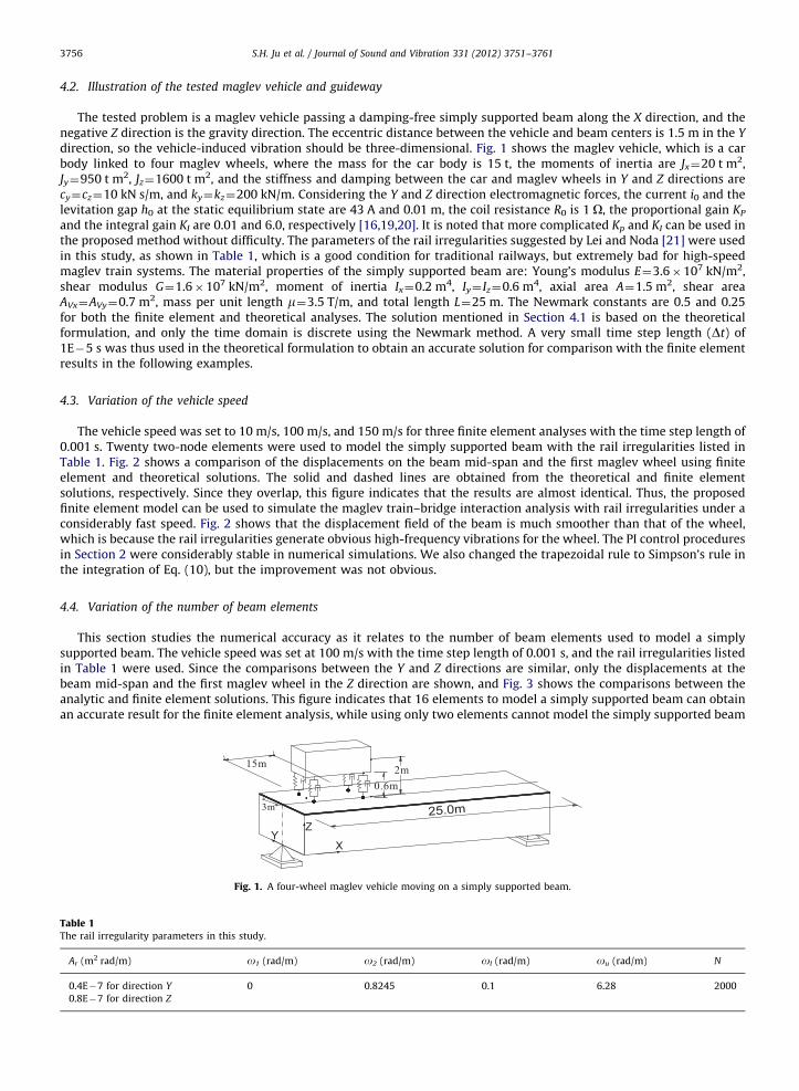
4.2. Illustration of the tested maglev vehicle and guideway

The tested problem is a maglev vehicle passing a damping-free simply supported beam along the X direction, and thenegative Z direction is the gravity direction. The eccentric distance between the vehicle and beam centers is 1.5 m in the Y

direction, so the vehicle-induced vibration should be three-dimensional. Fig. 1 shows the maglev vehicle, which is a carbody linked to four maglev wheels, where the mass for the car body is 15 t, the moments of inertia are Jx¼20 t m2,Jy¼950 t m2, Jz¼1600 t m2, and the stiffness and damping between the car and maglev wheels in Y and Z directions arecy¼cz¼10 kN s/m, and ky¼kz¼200 kN/m. Considering the Y and Z direction electromagnetic forces, the current i0 and thelevitation gap h0 at the static equilibrium state are 43 A and 0.01 m, the coil resistance R0 is 1 O, the proportional gain KP

and the integral gain KI are 0.01 and 6.0, respectively [16,19,20]. It is noted that more complicated Kp and KI can be used inthe proposed method without difficulty. The parameters of the rail irregularities suggested by Lei and Noda [21] were usedin this study, as shown in Table 1, which is a good condition for traditional railways, but extremely bad for high-speedmaglev train systems. The material properties of the simply supported beam are: Young’s modulus E¼3.6�107 kN/m2,shear modulus G¼1.6�107 kN/m2, moment of inertia Ix¼0.2 m4, Iy¼ Iz¼0.6 m4, axial area A¼1.5 m2, shear areaAVx¼AVy¼0.7 m2, mass per unit length m¼3.5 T/m, and total length L¼25 m. The Newmark constants are 0.5 and 0.25for both the finite element and theoretical analyses. The solution mentioned in Section 4.1 is based on the theoreticalformulation, and only the time domain is discrete using the Newmark method. A very small time step length (Dt) of1E�5 s was thus used in the theoretical formulation to obtain an accurate solution for comparison with the finite elementresults in the following examples.

4.3. Variation of the vehicle speed

The vehicle speed was set to 10 m/s, 100 m/s, and 150 m/s for three finite element analyses with the time step length of0.001 s. Twenty two-node elements were used to model the simply supported beam with the rail irregularities listed inTable 1. Fig. 2 shows a comparison of the displacements on the beam mid-span and the first maglev wheel using finiteelement and theoretical solutions. The solid and dashed lines are obtained from the theoretical and finite elementsolutions, respectively. Since they overlap, this figure indicates that the results are almost identical. Thus, the proposedfinite element model can be used to simulate the maglev train–bridge interaction analysis with rail irregularities under aconsiderably fast speed. Fig. 2 shows that the displacement field of the beam is much smoother than that of the wheel,which is because the rail irregularities generate obvious high-frequency vibrations for the wheel. The PI control proceduresin Section 2 were considerably stable in numerical simulations. We also changed the trapezoidal rule to Simpson’s rule inthe integration of Eq. (10), but the improvement was not obvious.

4.4. Variation of the number of beam elements

This section studies the numerical accuracy as it relates to the number of beam elements used to model a simplysupported beam. The vehicle speed was set at 100 m/s with the time step length of 0.001 s, and the rail irregularities listedin Table 1 were used. Since the comparisons between the Y and Z directions are similar, only the displacements at thebeam mid-span and the first maglev wheel in the Z direction are shown, and Fig. 3 shows the comparisons between theanalytic and finite element solutions. This figure indicates that 16 elements to model a simply supported beam can obtainan accurate result for the finite element analysis, while using only two elements cannot model the simply supported beam

XY

Z

3m

15m 2m0.6m

25.0m

Fig. 1. A four-wheel maglev vehicle moving on a simply supported beam.

Table 1The rail irregularity parameters in this study.

Ar (m2 rad/m) o1 (rad/m) o2 (rad/m) ol (rad/m) ou (rad/m) N

0.4E�7 for direction Y 0 0.8245 0.1 6.28 2000

0.8E�7 for direction Z

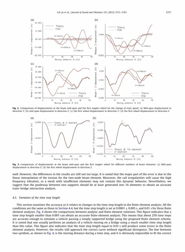
Fig. 2. Comparisons of displacements at the beam mid-span and the first maglev wheel for the change of train speed. (a) Mid-span displacement in

direction Y; (b) mid-span displacement in direction Z; (c) the first wheel displacement in direction Y; (d) the first wheel displacement in direction Z.

Fig. 3. Comparisons of displacements at the beam mid-span and the first maglev wheel for different numbers of beam elements. (a) Mid-span

displacement in direction Z; (b) the first wheel displacement in direction Z.

S.H. Ju et al. / Journal of Sound and Vibration 331 (2012) 3751–3761 3757

well. However, the differences in the results are still not too large. It is noted that the major part of the error is due to thelinear interpolation of the torsion for the two-node beam element. Moreover, the rail irregularities will cause the highfrequency vibration, so a mesh with insufficient elements may not contain this dynamic behavior. Nevertheless, wesuggest that the guideway between two supports should be at least generated into 16 elements to obtain an accuratetrain–bridge interaction analysis.

4.5. Variation of the time step length

This section examines the accuracy as it relates to changes in the time step length in the finite element analysis. All theconditions are the same as those in Section 4.4, but the time step length is set at 0.0001 s, 0.005 s, and 0.01 s for three finiteelement analyses. Fig. 4 shows the comparisons between analytic and finite element solutions. This figure indicates that atime step length smaller than 0.005 can obtain an accurate finite element analysis. This means that about 250 time stepsare accurate enough to simulate a vehicle passing a simply supported bridge using the proposed finite element scheme.It is noted that one usually performs an analysis of a vehicle moving on a bridge using a much smaller time step lengththan this value. This figure also indicates that the time step length equal to 0.01 s will produce some errors in the finiteelement analysis. However, the results still approach the correct curve without significant divergence. The line betweentwo symbols, as shown in Fig. 4, is the moving distance during a time step, and it is obviously impossible to fit the correct

Fig. 4. Comparisons of displacements at the beam mid-span and the first maglev wheel for the different time step lengths. (a) Mid-span displacement in

direction Z; (b) the first wheel displacement in direction Z.

1E-005 0.0001 0.001 0.01Time step length (s)

0

4

8

12

16

Ave

rage

iter

atio

n nu

mbe

r

Fig. 5. Average number of iterations per time step changing with time step length.

S.H. Ju et al. / Journal of Sound and Vibration 331 (2012) 3751–37613758

curve that has relatively small oscillations. Another important issue is that a large time step length may increase thenumber of iterations needed to achieve convergence. Fig. 5 shows changes in the time step length with the averagenumber of iterations needed to obtain convergence. This figure indicates that the finite element analysis is still efficientwhen one uses a large time step length, such as 0.002 s. Nevertheless, we suggest that a small time step length should beused to obtain more accurate numerical results.

5. Maglev train–bridge–soil interaction analysis

This section performs a maglev train–bridge–soil interaction analysis to demonstrate that the proposed model can beused to simulate complex practical problems with very large degrees of freedom. Moreover, the difference of the vibrationinduced by maglev and wheel/rail train systems is compared in this example. The maglev train has 12 carriages with thespeed of 300 km/h moving in the X direction, while the negative Z axis is the gravity direction. Each carriage contains fourbogies, and each bogie contains four maglev wheels. Fig. 6 shows the maglev train model, which contains spring–dampers,rigid bodies, and lumped masses. These components can be appropriately simulated using the wheels, lumped masses, andspring–damper elements mentioned in Section 3. The bridge is a series of simply supported beams with a span of 30 m.The bridge girders, foundation, and soil are exactly the same as those in Ju and Liao [22], so detailed explanations areomitted. The Newmark direct integration method and the consistent mass scheme were used to solve this problem withthe solution scheme of the Symmetric Successive Over-Relaxation (SSOR) preconditioned conjugated gradient method[23]. The finite element model is 1047.5 m long, 371 m wide, and 140 m deep, as shown in Fig. 7, with a maximum solidelement size of 2.5 m. The major part of the mesh is modeled by eight-node 3D solid elements for soil and the bridgefoundation, and the bridge piers and girders are modeled by two-node beam elements. The five mesh surfaces, excludingthe top surface, were modeled using the absorbing boundary condition [24] to avoid the fake wave reflection along themesh boundary. An illustration of these meshes can be found in Ju and Liao [22]. To connect the bridge and train, two linesof the slave nodes are generated with the master nodes along the beam nodes, where the first line is 1.25 m and 1 m indirections Y and Z, respectively, from the beam center, and the second line is 3.25 m and 1 m in directions Y and Z,respectively, from the beam center. The two lines of the slave nodes are the target nodes of the two-side maglev wheels,respectively. Fig. 7 shows a typical 3D finite element mesh, which contains 8,471,796 degrees of freedom. The time steplength is 0.002 s with 5000 time steps simulated. On average, three to four iterations are required to obtain the convergent

2.05 4.2 2.05 4.2 2.05 4.2 2.05

Unit = m

0.28

0.28

0.29

2.0

6.25 3.125 3.125 6.25

15 x 1.5625 (equal space)

1.253.25

1.0

2.0

1.0

Fig. 6. Maglev train dimensions and model containing spring–dampers, rigid bodies, and lumped masses.

Fig. 7. Finite element mesh (8,471,796 degrees of freedom).

Fig. 8. Finite element and experimental results of Z-direction vibrations on the center of the 4th carriage and at the bottom of the 20th bridge pier. (a) On

the center of the 4th carriage; (b) at the bottom of the 20th bridge pier.

S.H. Ju et al. / Journal of Sound and Vibration 331 (2012) 3751–3761 3759

finite element result within a time step, and the total computational time needed is about seven days using an Intel-2600Kcomputer.

The finite element results are presented in decibels (dB) using the 1/3 octave band in the frequency domain, which is aninternational standard in the semi-conductor industry [25]. Fig. 8 shows the finite element results for the Z directionvibrations on the center of the 4th carriage and at the bottom of the 20th bridge pier. The experimental results for theTaiwan high speed train moving in Tainan city are also plotted in this figure for a comparison, and those experimentalresults had been compared with the finite element results in good agreement [22]. The properties of the bridges, railirregularities and soils for the field experiment are the same as those of the maglev train analysis, and the only difference isthat one is a maglev train and the other is a wheel/rail train. Since the train speed was 300 km/h during the fieldexperiment, this train speed is also used in the maglev train analysis. In Fig. 9, the large vibration peak near 50 Hz for the

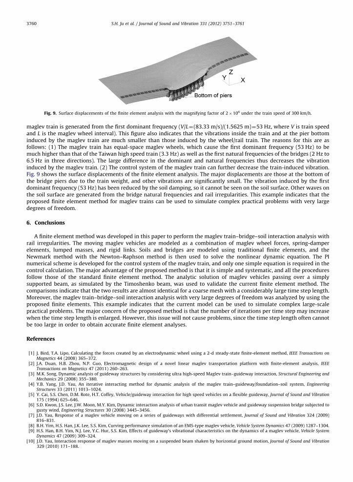
Fig. 9. Surface displacements of the finite element analysis with the magnifying factor of 2�106 under the train speed of 300 km/h.

S.H. Ju et al. / Journal of Sound and Vibration 331 (2012) 3751–37613760

maglev train is generated from the first dominant frequency (V/L¼(83.33 m/s)/(1.5625 m)¼53 Hz, where V is train speedand L is the maglev wheel interval). This figure also indicates that the vibrations inside the train and at the pier bottominduced by the maglev train are much smaller than those induced by the wheel/rail train. The reasons for this are asfollows: (1) The maglev train has equal-space maglev wheels, which cause the first dominant frequency (53 Hz) to bemuch higher than that of the Taiwan high speed train (3.3 Hz) as well as the first natural frequencies of the bridges (2 Hz to6.5 Hz in three directions). The large difference in the dominant and natural frequencies thus decreases the vibrationinduced by the maglev train. (2) The control system of the maglev train can further decrease the train-induced vibration.Fig. 9 shows the surface displacements of the finite element analysis. The major displacements are those at the bottom ofthe bridge piers due to the train weight, and other vibrations are significantly small. The vibration induced by the firstdominant frequency (53 Hz) has been reduced by the soil damping, so it cannot be seen on the soil surface. Other waves onthe soil surface are generated from the bridge natural frequencies and rail irregularities. This example indicates that theproposed finite element method for maglev trains can be used to simulate complex practical problems with very largedegrees of freedom.

6. Conclusions

A finite element method was developed in this paper to perform the maglev train–bridge–soil interaction analysis withrail irregularities. The moving maglev vehicles are modeled as a combination of maglev wheel forces, spring-damperelements, lumped masses, and rigid links. Soils and bridges are modeled using traditional finite elements, and theNewmark method with the Newton–Raphson method is then used to solve the nonlinear dynamic equation. The PInumerical scheme is developed for the control system of the maglev train, and only one simple equation is required in thecontrol calculation. The major advantage of the proposed method is that it is simple and systematic, and all the proceduresfollow those of the standard finite element method. The analytic solution of maglev vehicles passing over a simplysupported beam, as simulated by the Timoshenko beam, was used to validate the current finite element method. Thecomparisons indicate that the two results are almost identical for a coarse mesh with a considerably large time step length.Moreover, the maglev train–bridge–soil interaction analysis with very large degrees of freedom was analyzed by using theproposed finite elements. This example indicates that the current model can be used to simulate complex large-scalepractical problems. The major concern of the proposed method is that the number of iterations per time step may increasewhen the time step length is enlarged. However, this issue will not cause problems, since the time step length often cannotbe too large in order to obtain accurate finite element analyses.

References

[1] J. Bird, T.A. Lipo, Calculating the forces created by an electrodynamic wheel using a 2-d steady-state finite-element method, IEEE Transactions onMagnetics 44 (2008) 365–372.

[2] J.A. Duan, H.B. Zhou, N.P. Guo, Electromagnetic design of a novel linear maglev transportation platform with finite-element analysis, IEEETransactions on Magnetics 47 (2011) 260–263.

[3] M.K. Song, Dynamic analysis of guideway structures by considering ultra high-speed Maglev train–guideway interaction, Structural Engineering andMechanics 29 (2008) 355–380.

[4] Y.B. Yang, J.D. Yau, An iterative interacting method for dynamic analysis of the maglev train–guideway/foundation–soil system, EngineeringStructures 33 (2011) 1013–1024.

[5] Y. Cai, S.S. Chen, D.M. Rote, H.T. Coffey, Vehicle/guideway interaction for high speed vehicles on a flexible guideway, Journal of Sound and Vibration175 (1994) 625–646.

[6] S.D. Kwon, J.S. Lee, J.W. Moon, M.Y. Kim, Dynamic interaction analysis of urban transit maglev vehicle and guideway suspension bridge subjected togusty wind, Engineering Structures 30 (2008) 3445–3456.

[7] J.D. Yau, Response of a maglev vehicle moving on a series of guideways with differential settlement, Journal of Sound and Vibration 324 (2009)816–831.

[8] B.H. Yim, H.S. Han, J.K. Lee, S.S. Kim, Curving performance simulation of an EMS-type maglev vehicle, Vehicle System Dynamics 47 (2009) 1287–1304.[9] H.S. Han, B.H. Yim, N.J. Lee, Y.C. Hur, S.S. Kim, Effects of guideway’s vibrational characteristics on the dynamics of a maglev vehicle, Vehicle System

Dynamics 47 (2009) 309–324.[10] J.D. Yau, Interaction response of maglev masses moving on a suspended beam shaken by horizontal ground motion, Journal of Sound and Vibration

329 (2010) 171–188.

S.H. Ju et al. / Journal of Sound and Vibration 331 (2012) 3751–3761 3761

[11] C.Y. Hu, K.C. Chen, J.S. Chen, Dynamic interaction of a distributed supported guideway and a asymmetrical multimagnet suspension vehicle withunbalanced mass, Journal of Mechanics 26 (2010) 1–14.

[12] J. Shi, Q.C. Wei, Y. Zhao, Analysis of dynamic response of the high-speed EMS maglev vehicle/guideway coupling system with random irregularity,Vehicle System Dynamics 45 (2007) 1077–1095.

[13] A. Bittar, R.M. Sales, H-2 and H-infinity control for MagLev vehicles, IEEE Control Systems 18 (1998) 18–25.[14] H.D. Taghirad, M. Abrishamchian, R. Ghabcheloo, Electromagnetic levitation system: an experimental approach, The Seventh International Conference

in Elevtrical Engineering, Power System Vol, Tehran, Iran (1998).[15] F.T.K. Au, J.J. Wang, Y.K. Cheung, Impact study of cable-stayed railway bridges with random rail irregularities, Engineering Structures 24 (2002)

529–541.[16] J.D. Yau, Vibration control of maglev vehicles traveling over a flexible guideway, Journal of Sound and Vibration 321 (2009) 184–200.[17] S.H. Ju, H.D. Lin, C.C. Hsueh, S.L. Wang, A simple finite element model for vibration analyses induced by moving vehicles, International Journal for

Numerical Method in Engineering 68 (2006) 1232–1256.[18] S.H. Ju, Vibration analysis of 3D Timoshenko beams subjected to moving vehicles, Journal Engineering Mechanics, ASCE 137 (2011) 713–784.[19] C.F. Zhao, W.M. Zhai, Maglev vehicle/guideway vertical random response and ride quality, Vehicle System Dynamics 38 (2002) 185–210.[20] G. Bohn, G. Steinmetz, The electromagnetic levitation and guidance technology of the ‘transrapid’ test facility EMSland, IEEE Transactions on

Magnetics 20 (1984) 1666–1671.[21] X. Lei, N.A. Noda, Analyses of dynamic response of vehicle and track coupling system with random irregularity of track vertical profile, Journal of

Sound and Vibration 258 (2002) 147–165.[22] S.H. Ju, J.R. Liao, Error study of rail/wheel point contact method for moving trains with rail roughness, Computers and Structures 88 (2010) 813–824.[23] S.H. Ju, A simple OpenMP scheme for parallel iteration solvers in finite element analysis, CMES — Computer Modeling in Engineering & Sciences 64

(2010) 91–109.[24] S.H. Ju, Y.M. Wang, Time-dependent absorbing boundary conditions for elastic wave propagation, International Journal for Numerical Method in

Engineering 50 (2001) 2159–2174.[25] C.G. Gordon, Generic criteria for vibration sensitive equipment, SPIE1619 (1991) 71–75.