a finite difference solution of the regularized long-wave …
TRANSCRIPT
A FINITE DIFFERENCE SOLUTION OF THE REGULARIZEDLONG-WAVE EQUATION
S. KUTLUAY AND A. ESEN
Received 26 July 2005; Accepted 24 January 2006
A linearized implicit finite difference method to obtain numerical solution of the one-dimensional regularized long-wave (RLW) equation is presented. The performance andthe accuracy of the method are illustrated by solving three test examples of the problem:a single solitary wave, two positive solitary waves interaction, and an undular bore. Theobtained results are presented and compared with earlier work.
Copyright © 2006 S. Kutluay and A. Esen. This is an open access article distributed underthe Creative Commons Attribution License, which permits unrestricted use, distribution,and reproduction in any medium, provided the original work is properly cited.
1. Introduction
In this study, we will consider the one-dimensional RLW equation
∂U
∂t+∂U
∂x+ εU
∂U
∂x−μ
∂
∂t
(∂2U
∂x2
)= 0, (1.1)
with the physical boundary conditions U → 0 as x→±∞, where t is time, x is the spacecoordinate, U(x, t) is the wave amplitude, and ε and μ are positive parameters. The RLWequation (1.1) was first introduced by Peregrine [1] to describe the development of an un-dular bore. This equation is one of the most important nonlinear wave equations whichcan be used to model a large number of problems arising in various areas of applied sci-ences [2, 3]. The RLW equation has been solved analytically for a restricted set of bound-ary and initial conditions. Therefore, the numerical solution of the RLW equation hasbeen the subject of many papers. Various numerical techniques particularly including fi-nite difference [4–8], finite element [9–19], and spectral [20–23] methods have been usedfor the solution of the RLW equation.
In this paper, we have used a linearized implicit finite difference method to investigatethe motion of a single solitary wave, development of two positive solitary waves interac-tion, and an undular bore for the RLW equation (1.1).
Hindawi Publishing CorporationMathematical Problems in EngineeringVolume 2006, Article ID 85743, Pages 1–14DOI 10.1155/MPE/2006/85743

2 Regularized long-wave equation
2. Method of solution
For the numerical treatment, the spatial variable x of the problem is restricted over an in-terval a≤ x ≤ b. In this study, we consider the RLW equation (1.1) with the homogeneousboundary conditions
U(a, t)= 0, t > 0, U(b, t)= 0, t > 0, (2.1)
and the initial condition
U(x,0)= f (x), a≤ x ≤ b, (2.2)
where f (x) is a prescribed function.The solution domain a ≤ x ≤ b, t > 0 is divided into subintervals Δx in the direction
of the spatial variable x and Δt in the direction of time t such that xi = iΔx, i = 0(1)N(NΔx = b− a); t j = jΔt, j = 0(1)J , and the numerical solution of U at the grid point(iΔx, jΔt) is denoted by Ui, j .
In the finite difference method, the dependent variable and its derivatives are approx-imated by the finite difference approximation. This approximation will lead to either asingle explicit equation or a system of difference equations. Applying the classical im-plicit finite difference method to nonlinear problems normally gives nonlinear system ofequations which cannot be solved directly.
Equation (1.1) can be written as
∂U
∂t+∂U
∂x+ε
2∂U2
∂x−μ
∂
∂t
(∂2U
∂x2
)= 0. (2.3)
Using the forward difference approximation for ∂U/∂t, the Crank-Nicolson difference ap-proximation for ∂U/∂x and ∂U2/∂x, and the central difference approximation for ∂2U/∂x2
at the point (i, j + 1),
∂U
∂t∼= Ui, j+1−Ui, j
Δt,
∂U
∂x∼= 1
2
{1
2Δx
(Ui+1, j+1−Ui−1, j+1
)+
12Δx
(Ui+1, j −Ui−1, j
)},
∂U2
∂x∼= 1
2
{1
2Δx
(U2
i+1, j+1−U2i−1, j+1
)+
12Δx
(U2
i+1, j −U2i−1, j
)},
∂2U
∂x2∼= 1
(Δx)2
(Ui+1, j − 2Ui, j +Ui−1, j
),
(2.4)
respectively, (2.3) yields the system of algebraic equations
Ui, j+1−Ui, j
Δt+
14Δx
(Ui+1, j+1−Ui−1, j+1 +Ui+1, j −Ui−1, j
)
+ε
8Δx
(U2
i+1, j+1−U2i−1, j+1 +U2
i+1, j −U2i−1, j
)
− μ
Δt(Δx)2
(Ui+1, j+1− 2Ui, j+1 +Ui−1, j+1−Ui+1, j + 2Ui, j −Ui−1, j
)= 0
(2.5)
S. Kutluay and A. Esen 3
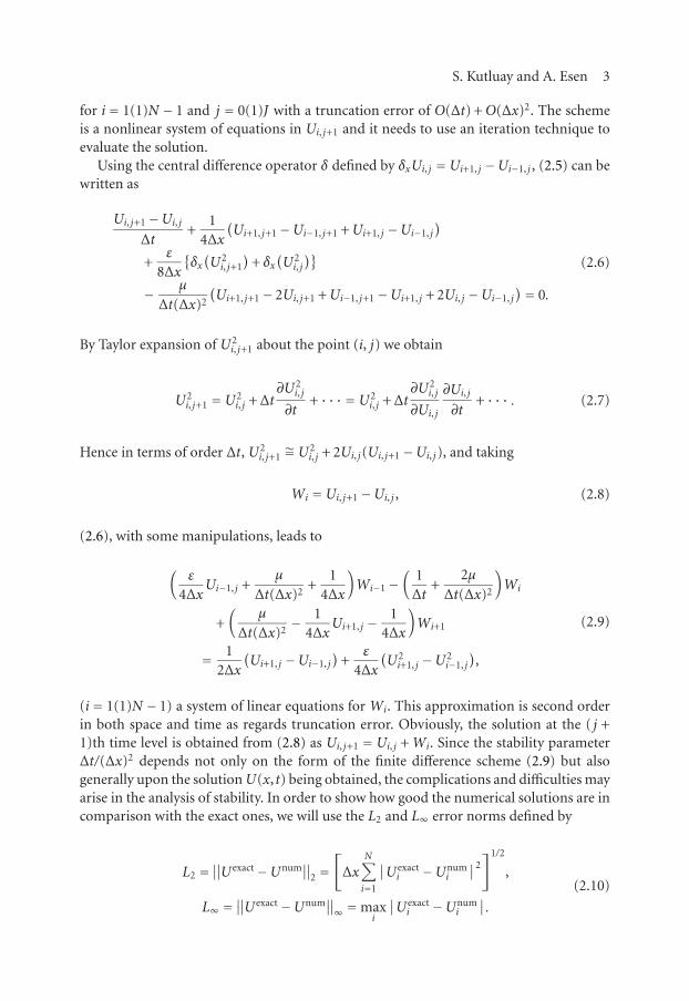
for i = 1(1)N − 1 and j = 0(1)J with a truncation error of O(Δt) +O(Δx)2. The schemeis a nonlinear system of equations in Ui, j+1 and it needs to use an iteration technique toevaluate the solution.
Using the central difference operator δ defined by δxUi, j =Ui+1, j −Ui−1, j , (2.5) can bewritten as
Ui, j+1−Ui, j
Δt+
14Δx
(Ui+1, j+1−Ui−1, j+1 +Ui+1, j −Ui−1, j
)
+ε
8Δx
{δx(U2
i, j+1
)+ δx
(U2
i, j
)}
− μ
Δt(Δx)2
(Ui+1, j+1− 2Ui, j+1 +Ui−1, j+1−Ui+1, j + 2Ui, j −Ui−1, j
)= 0.
(2.6)
By Taylor expansion of U2i, j+1 about the point (i, j) we obtain
U2i, j+1 =U2
i, j +Δt∂U2
i, j
∂t+ ··· =U2
i, j +Δt∂U2
i, j
∂Ui, j
∂Ui, j
∂t+ ··· . (2.7)
Hence in terms of order Δt, U2i, j+1
∼=U2i, j + 2Ui, j(Ui, j+1−Ui, j), and taking
Wi =Ui, j+1−Ui, j , (2.8)
(2.6), with some manipulations, leads to
(ε
4ΔxUi−1, j +
μ
Δt(Δx)2+
14Δx
)Wi−1−
(1Δt
+2μ
Δt(Δx)2
)Wi
+(
μ
Δt(Δx)2− 1
4ΔxUi+1, j − 1
4Δx
)Wi+1
= 12Δx
(Ui+1, j −Ui−1, j
)+
ε
4Δx
(U2
i+1, j −U2i−1, j
),
(2.9)
(i= 1(1)N − 1) a system of linear equations for Wi. This approximation is second orderin both space and time as regards truncation error. Obviously, the solution at the ( j +1)th time level is obtained from (2.8) as Ui, j+1 = Ui, j +Wi. Since the stability parameterΔt/(Δx)2 depends not only on the form of the finite difference scheme (2.9) but alsogenerally upon the solutionU(x, t) being obtained, the complications and difficulties mayarise in the analysis of stability. In order to show how good the numerical solutions are incomparison with the exact ones, we will use the L2 and L∞ error norms defined by
L2 =∥∥Uexact−Unum
∥∥2 =
[Δx
N∑i=1
∣∣Uexacti −Unum
i
∣∣2]1/2
,
L∞ =∥∥Uexact−Unum
∥∥∞ =maxi
∣∣Uexacti −Unum
i
∣∣.(2.10)

4 Regularized long-wave equation
3. Numerical examples and results
All computations were executed on a Pentium 4 PC in the Fortran code using doubleprecision arithmetic. The RLW equation (1.1) satisfies only three conservation laws givenas
I1 =∫ +∞
−∞Udx � Δx
N∑i=1
Ui, j ,
I2 =∫ +∞
−∞
[U2 +μ
(Ux)2]dx � Δx
N∑i=1
[(Ui, j)2
+μ((Ux)i, j
)2],
I3 =∫ +∞
−∞
[U3 + 3U2]dx � Δx
N∑i=1
[(Ui, j)3
+ 3(Ui, j)2]
(3.1)
which respectively correspond to mass, momentum, and energy [24]. In the simulationsthe invariants I1, I2, and I3 are monitored to check the conservation of the numericalscheme. For the computation of Ux in (3.1), we used a central finite difference approxi-mation.
To implement the performance of the method, three test problems will be considered:the motion of a single solitary wave, the interaction of two positive solitary waves, andthe undular bore.
3.1. The motion of a single solitary wave. We first consider (1.1) with the boundaryconditions U → 0 as x→±∞ and the initial condition
U(x,0)= 3c sech2(k(x− x0)). (3.2)
The exact solution of this problem is
U(x, t)= 3c sech2(k(x− vt− x0)). (3.3)
This solution corresponds to the motion of a single solitary wave with amplitude 3cand width k, initially centered at x0, where v = 1 + εc is the wave velocity and k = (1/2)(εc/μv)1/2. This solution will also be used over an interval a≤ x ≤ b. For this problemthe theoretical values of the invariants are [14]
I1 = 6ck
, I2 = 12c2
k+
48kc2μ
5, I3 = 36c2
k+
144c3
5k(3.4)
which are recorded throughout the simulations. For the purpose of comparing with theearlier work, all computations are done for the parameters ε = 1, μ= 1, and x0 = 0.
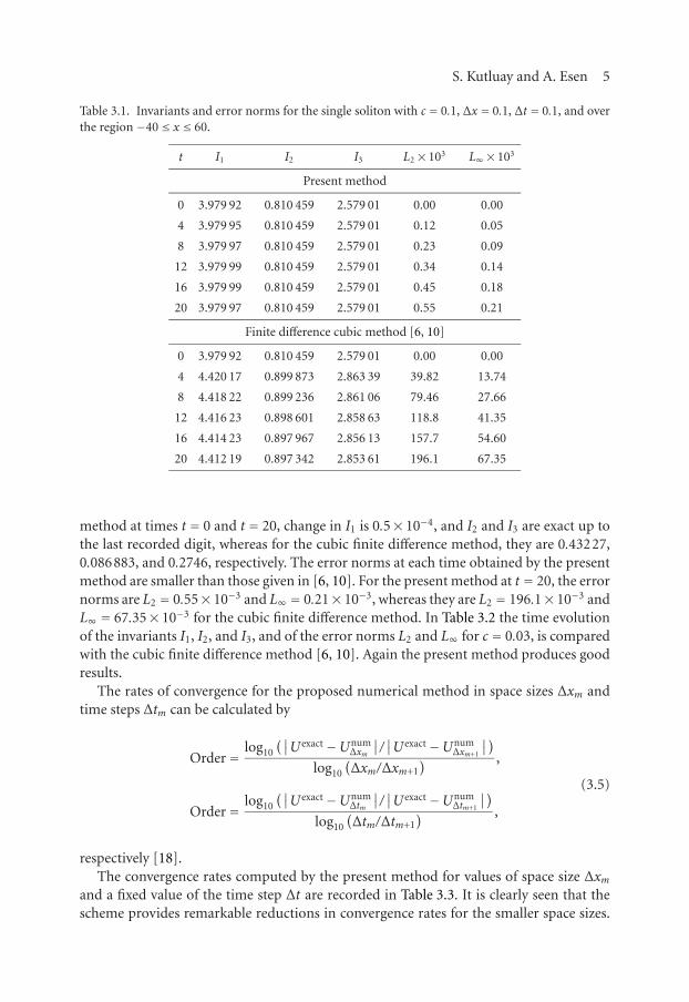
Table 3.1 displays a comparison of the values of the invariants and error norms ob-tained by the present method with those obtained using the cubic finite difference methoddeveloped by Jain et al. [6] and implemented by Gardner et al. [10] for c = 0.1. As it is seenfrom the table, the numerical values of invariants obtained from (3.1) are in very goodagreement with their analytical values obtained from (3.4). The quantities in the invari-ants remain almost constant during the computer run. For the proposed finite difference
S. Kutluay and A. Esen 5
Table 3.1. Invariants and error norms for the single soliton with c = 0.1, Δx = 0.1, Δt = 0.1, and overthe region −40≤ x ≤ 60.
t I1 I2 I3 L2× 103 L∞ × 103
Present method
0 3.979 92 0.810 459 2.579 01 0.00 0.00
4 3.979 95 0.810 459 2.579 01 0.12 0.05
8 3.979 97 0.810 459 2.579 01 0.23 0.09
12 3.979 99 0.810 459 2.579 01 0.34 0.14
16 3.979 99 0.810 459 2.579 01 0.45 0.18
20 3.979 97 0.810 459 2.579 01 0.55 0.21
Finite difference cubic method [6, 10]
0 3.979 92 0.810 459 2.579 01 0.00 0.00
4 4.420 17 0.899 873 2.863 39 39.82 13.74
8 4.418 22 0.899 236 2.861 06 79.46 27.66
12 4.416 23 0.898 601 2.858 63 118.8 41.35
16 4.414 23 0.897 967 2.856 13 157.7 54.60
20 4.412 19 0.897 342 2.853 61 196.1 67.35
method at times t = 0 and t = 20, change in I1 is 0.5× 10⁻⁴, and I2 and I3 are exact up tothe last recorded digit, whereas for the cubic finite difference method, they are 0.43227,0.086883, and 0.2746, respectively. The error norms at each time obtained by the presentmethod are smaller than those given in [6, 10]. For the present method at t = 20, the errornorms are L2 = 0.55× 10⁻³ and L∞ = 0.21× 10⁻³, whereas they are L2 = 196.1× 10⁻³ andL∞ = 67.35× 10⁻³ for the cubic finite difference method. In Table 3.2 the time evolutionof the invariants I1, I2, and I3, and of the error norms L2 and L∞ for c = 0.03, is comparedwith the cubic finite difference method [6, 10]. Again the present method produces goodresults.
The rates of convergence for the proposed numerical method in space sizes Δxm andtime steps Δtm can be calculated by
Order= log10
(∣∣Uexact−UnumΔxm
∣∣/∣∣Uexact−UnumΔxm+1
∣∣)log10
(Δxm/Δxm+1
) ,
Order= log10
(∣∣Uexact−UnumΔtm
∣∣/∣∣Uexact−UnumΔtm+1
∣∣)log10
(Δtm/Δtm+1
) ,
(3.5)
respectively [18].The convergence rates computed by the present method for values of space size Δxm
and a fixed value of the time step Δt are recorded in Table 3.3. It is clearly seen that thescheme provides remarkable reductions in convergence rates for the smaller space sizes.
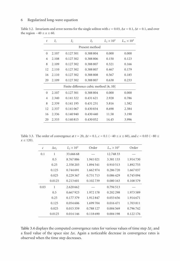
6 Regularized long-wave equation
Table 3.2. Invariants and error norms for the single soliton with c = 0.03, Δx = 0.1, Δt = 0.1, and overthe region −40≤ x ≤ 60.
t I1 I2 I3 L2× 103 L∞ × 103
Present method
0 2.107 0.127 301 0.388 804 0.000 0.000
4 2.108 0.127 302 0.388 806 0.150 0.123
8 2.109 0.127 302 0.388 807 0.321 0.166
12 2.110 0.127 302 0.388 807 0.467 0.179
16 2.110 0.127 302 0.388 808 0.567 0.185
20 2.109 0.127 302 0.388 807 0.638 0.233
Finite difference cubic method [6, 10]
0 2.107 0.127 301 0.388 804 0.000 0.000
4 2.340 0.141 322 0.431 621 2.928 0.786
8 2.339 0.141 195 0.431 231 5.816 1.582
12 2.337 0.141 067 0.430 834 8.698 2.384
16 2.336 0.140 940 0.430 440 11.58 3.190
20 2.333 0.140 815 0.430 052 14.45 3.996
Table 3.3. The order of convergence at t = 20, Δt = 0.1, c = 0.1 (−40≤ x ≤ 60), and c = 0.03 (−80≤x ≤ 120).
c Δxj L2× 103 Order L∞ × 103 Order
0.1 1 33.666 68 — 12.748 33 —
0.5 8.767 886 1.941 021 3.381 133 1.914 730
0.25 2.358 203 1.894 541 0.910 513 1.892 755
0.125 0.744 691 1.662 974 0.286 720 1.667 037
0.025 0.229 367 0.731 713 0.086 429 0.745 094
0.0125 0.213 601 0.102 739 0.080 163 0.108 579
0.03 1 2.620 662 — 0.794 513 —
0.5 0.667 923 1.972 178 0.202 298 1.973 589
0.25 0.177 379 1.912 847 0.053 656 1.914 671
0.125 0.054 606 1.699 704 0.016 471 1.703 811
0.025 0.015 359 0.788 127 0.004 569 0.796 742
0.0125 0.014 146 0.118 690 0.004 198 0.122 176
Table 3.4 displays the computed convergence rates for various values of time step Δt j anda fixed value of the space size Δx. Again a noticeable decrease in convergence rates isobserved when the time step decreases.

S. Kutluay and A. Esen 7
Table 3.4. The order of convergence at t = 20, Δx = 0.1, c = 0.1 (−40≤ x ≤ 60), and c = 0.03 (−80≤x ≤ 120).
c Δt j L2× 103 Order L∞ × 103 Order
0.1 1 20.292 460 — 7.618 319 —
0.5 5.461 549 1.893 562 2.062 621 1.884 994
0.25 1.631 432 1.743 171 6.197 000 1.734 837
0.125 0.666 724 1.290 977 0.255 439 1.278 591
0.025 0.358 400 0.385 679 0.138 568 0.380 022
0.0125 0.348 799 0.039 175 0.134 914 0.038 554
0.03 1 1.380 075 — 0.411 315 —
0.5 0.367 151 1.910 301 0.109 469 1.909 721
0.25 0.111 587 1.718 205 0.033 363 1.714 201
0.125 0.047 558 1.230 409 0.014 296 1.222 637
0.025 0.027 068 0.350 183 0.008 194 0.345 821
0.0125 0.026 428 0.034 521 0.008 003 0.034 027
The profiles of the solitary waves at times t = 0 and t = 20 and the error distributions ofthe analytical and numerical solutions at t = 20 for c = 0.1 with the range −40≤ x ≤ 60and for c = 0.03 with the range −80 ≤ x ≤ 120, Δx = 0.125 and Δt = 0.1 are shown inFigure 3.1. For c = 0.1, the amplitude is 0.3 at time t = 0 while it is 0.299919 at time t = 20(Figure 3.1(a)) and so the relative change in the amplitude is about 0.027%. It is seen thatthe maximum error is about between −4× 10⁻³ and 4× 10⁻³ (Figure 3.1(b)). For c =0.03, the amplitude is 0.09 at time t = 0 while it is 0.089997 at time t = 20 (Figure 3.1(c))and so the relative change in the amplitude is about 0.0033%. It is observed that themaximum error is about between −6× 10⁻⁴ and 6× 10⁻⁴ (Figure 3.1(d)).
3.2. The interaction of two positive solitary waves. We secondly consider (1.1) with theboundary conditions U → 0 as x→±∞ and the initial condition [17]
U(x,0)=2∑j=1
3Aj sech2(kj(x− xj))
, (3.6)
where Aj = 4k2j /(1− 4k2
j ) ( j = 1,2).For the simulation, all computations are done for the parameters k1 = 0.4, x1 = 15,
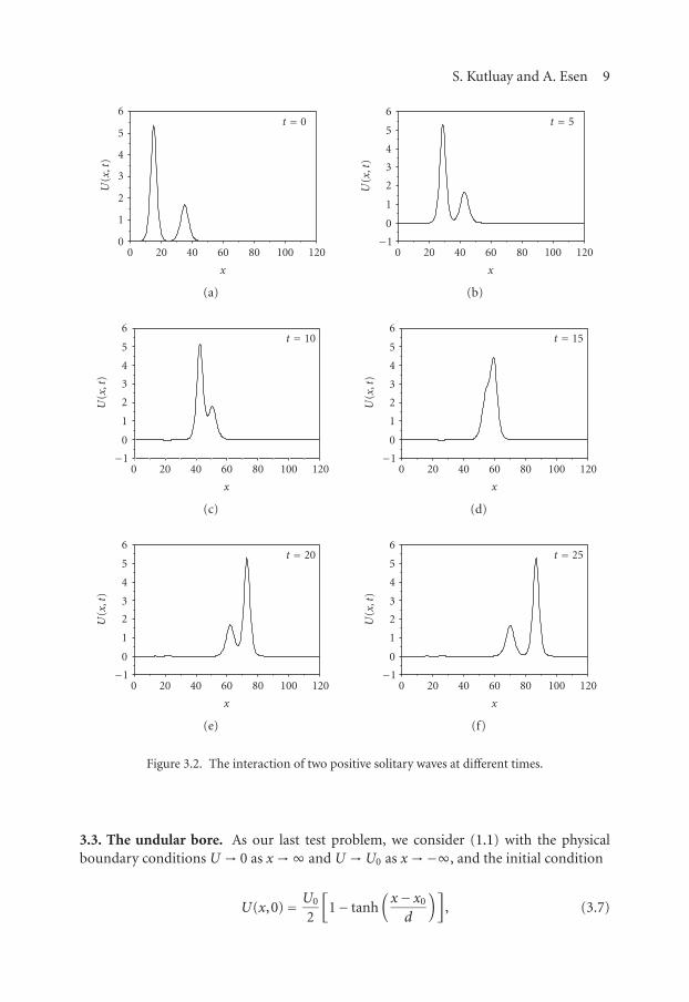
k2 = 0.3, x2 = 35, ε = 1, μ = 1, Δx = 0.3, and Δt = 0.1 over the region 0 ≤ x ≤ 120. Theexperiment was run from t = 0 to t = 25 to allow the interaction to take place. Figure 3.2shows the interaction of two positive solitary waves. As it is seen from the figure, at t = 0a solitary wave with larger amplitude is on the left of the other solitary wave with smalleramplitude. The larger wave catches up with the smaller one as the time increases. At t = 0,

8 Regularized long-wave equation
−40 −20 0 20 40 60
x
0
0.1
0.2
0.3
U(x,t
)
t = 0 t = 20
(a)
−40 −20 0 20 40 60
x
−6
−4
−2
0
2
4
6×10⁻³
Ero
rr
(b)
−80 −40 0 40 80 120
x
0
0.3
0.6
0.9×10⁻¹
U(x,t
)
t = 0 t = 20
(c)
−80 −40 0 40 80 120
x
−8
−6
−4
−2
0
2
4
6
8×10⁻⁴
Ero
rr
(d)
Figure 3.1. Solitary wave profiles at t = 0,20 and error (error = exact-numerical) distributions att = 20.
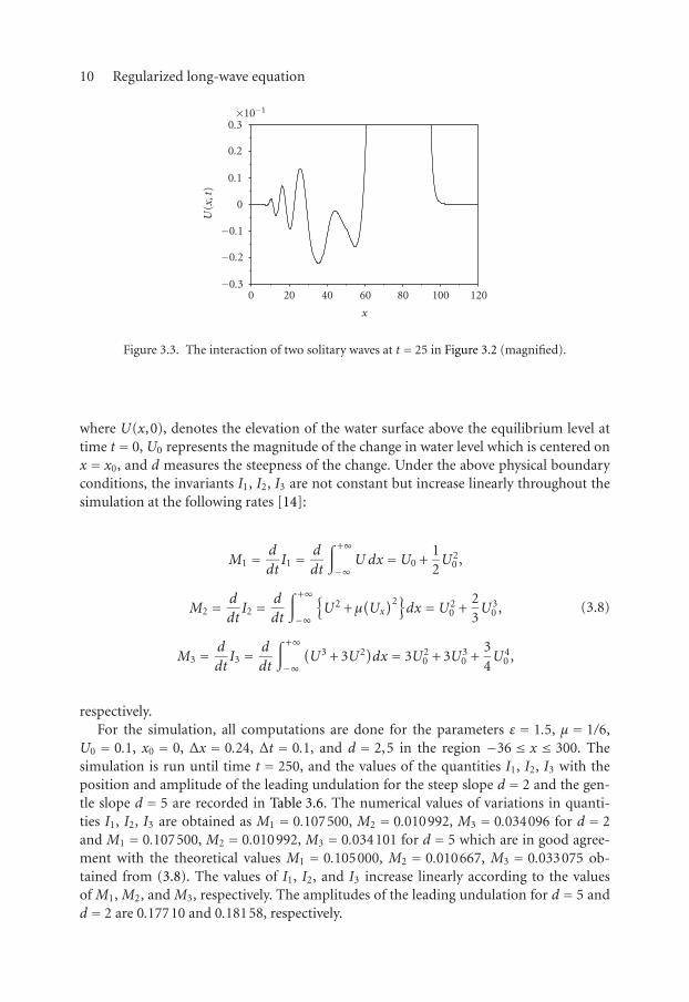
the amplitude of the larger solitary wave is 5.33338 while the amplitude of the smaller oneis 1.68598, whereas at t = 25, the amplitude of the larger solitary wave is 5.30235 at thepoint x = 86.7 while the amplitude of the smaller one is 1.67157 at the point x = 69.9. Anoscillation of small amplitude trailing behind the solitary waves was observed. In orderto see this oscillation occurring behind the waves in Figure 3.2 at time t = 25, the scale ofthe figure is magnified as in Figure 3.3. It is clearly seen that an oscillation of amplitude∼ 2.2× 10⁻² is trailing behind the solitary waves.
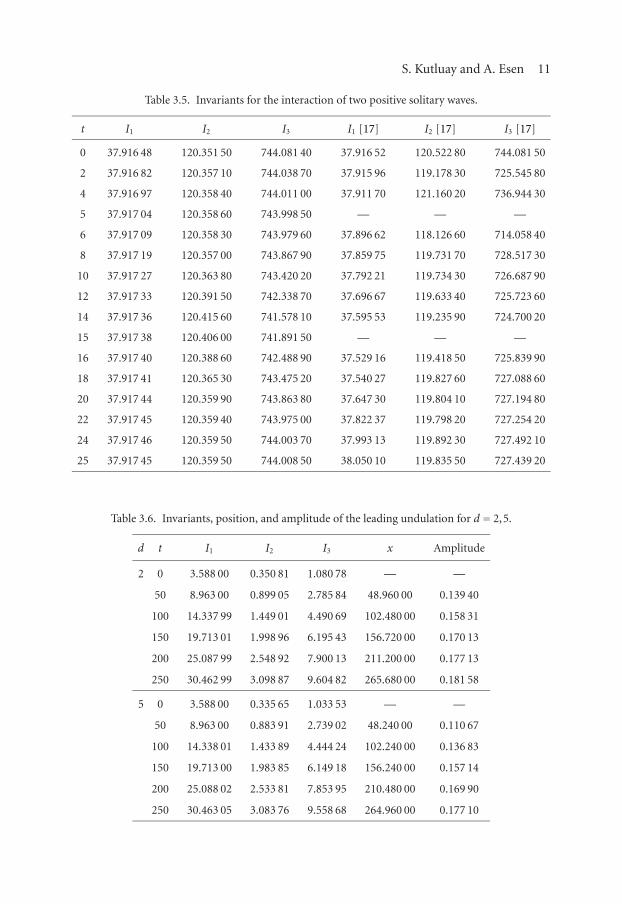
Table 3.5 displays a comparison of the values of the invariants obtained by the presentmethod with those obtained in [17]. It is observed that the obtained values of the in-variants remain almost constant during the computer run. At times t = 0 and t = 25, therelative changes in the invariants I1, I2, and I3 for the present method are respectively2.558× 10−3%, 6.647× 10⁻³%, and 9.797× 10⁻³% whereas they are 0.352%, 0.570%,and 2.237% for the cubic B-spline collocation finite element method given in [17]. It isclearly seen that each of the conserved quantities obtained by the present method is verywell preserved.
S. Kutluay and A. Esen 9
0 20 40 60 80 100 120
x
0
1
2
3
4
5
6U
(x,t
)
t = 0
(a)
0 20 40 60 80 100 120
x
−1
0
1
2
3
4
5
6
U(x,t
)
t = 5
(b)
0 20 40 60 80 100 120
x
−1
0
1
2
3
4
5
6
U(x,t
)
t = 10
(c)
0 20 40 60 80 100 120
x
−1
0
1
2
3
4
5
6
U(x,t
)
t = 15
(d)
0 20 40 60 80 100 120
x
−1
0
1
2
3
4
5
6
U(x,t
)
t = 20
(e)
0 20 40 60 80 100 120
x
−1
0
1
2
3
4
5
6
U(x,t
)
t = 25
(f)
Figure 3.2. The interaction of two positive solitary waves at different times.
3.3. The undular bore. As our last test problem, we consider (1.1) with the physicalboundary conditions U → 0 as x→∞ and U →U0 as x→−∞, and the initial condition
U(x,0)= U0
2
[1− tanh
(x− x0
d
)], (3.7)
10 Regularized long-wave equation
0 20 40 60 80 100 120
x
−0.3
−0.2
−0.1
0
0.1
0.2
0.3×10⁻¹
U(x,t
)
Figure 3.3. The interaction of two solitary waves at t = 25 in Figure 3.2 (magnified).
where U(x,0), denotes the elevation of the water surface above the equilibrium level attime t = 0, U0 represents the magnitude of the change in water level which is centered onx = x0, and d measures the steepness of the change. Under the above physical boundaryconditions, the invariants I1, I2, I3 are not constant but increase linearly throughout thesimulation at the following rates [14]:
M1 = d
dtI1 = d
dt
∫ +∞
−∞Udx =U0 +
12U2
0 ,
M2 = d
dtI2 = d
dt
∫ +∞
−∞
{U2 +μ
(Ux)2}dx =U2
0 +23U3
0 ,
M3 = d
dtI3 = d
dt
∫ +∞
−∞
(U3 + 3U2)dx = 3U2
0 + 3U30 +
34U4
0 ,
(3.8)
respectively.For the simulation, all computations are done for the parameters ε = 1.5, μ = 1/6,
U0 = 0.1, x0 = 0, Δx = 0.24, Δt = 0.1, and d = 2,5 in the region −36 ≤ x ≤ 300. Thesimulation is run until time t = 250, and the values of the quantities I1, I2, I3 with theposition and amplitude of the leading undulation for the steep slope d = 2 and the gen-tle slope d = 5 are recorded in Table 3.6. The numerical values of variations in quanti-ties I1, I2, I3 are obtained as M1 = 0.107500, M2 = 0.010992, M3 = 0.034096 for d = 2and M1 = 0.107500, M2 = 0.010992, M3 = 0.034101 for d = 5 which are in good agree-ment with the theoretical values M1 = 0.105000, M2 = 0.010667, M3 = 0.033075 ob-tained from (3.8). The values of I1, I2, and I3 increase linearly according to the valuesof M1, M2, and M3, respectively. The amplitudes of the leading undulation for d = 5 andd = 2 are 0.17710 and 0.18158, respectively.
S. Kutluay and A. Esen 11
Table 3.5. Invariants for the interaction of two positive solitary waves.
t I1 I2 I3 I1 [17] I2 [17] I3 [17]
0 37.916 48 120.351 50 744.081 40 37.916 52 120.522 80 744.081 50
2 37.916 82 120.357 10 744.038 70 37.915 96 119.178 30 725.545 80
4 37.916 97 120.358 40 744.011 00 37.911 70 121.160 20 736.944 30
5 37.917 04 120.358 60 743.998 50 — — —
6 37.917 09 120.358 30 743.979 60 37.896 62 118.126 60 714.058 40
8 37.917 19 120.357 00 743.867 90 37.859 75 119.731 70 728.517 30
10 37.917 27 120.363 80 743.420 20 37.792 21 119.734 30 726.687 90
12 37.917 33 120.391 50 742.338 70 37.696 67 119.633 40 725.723 60
14 37.917 36 120.415 60 741.578 10 37.595 53 119.235 90 724.700 20
15 37.917 38 120.406 00 741.891 50 — — —
16 37.917 40 120.388 60 742.488 90 37.529 16 119.418 50 725.839 90
18 37.917 41 120.365 30 743.475 20 37.540 27 119.827 60 727.088 60
20 37.917 44 120.359 90 743.863 80 37.647 30 119.804 10 727.194 80
22 37.917 45 120.359 40 743.975 00 37.822 37 119.798 20 727.254 20
24 37.917 46 120.359 50 744.003 70 37.993 13 119.892 30 727.492 10
25 37.917 45 120.359 50 744.008 50 38.050 10 119.835 50 727.439 20
Table 3.6. Invariants, position, and amplitude of the leading undulation for d = 2,5.
d t I1 I2 I3 x Amplitude
2 0 3.588 00 0.350 81 1.080 78 — —
50 8.963 00 0.899 05 2.785 84 48.960 00 0.139 40
100 14.337 99 1.449 01 4.490 69 102.480 00 0.158 31
150 19.713 01 1.998 96 6.195 43 156.720 00 0.170 13
200 25.087 99 2.548 92 7.900 13 211.200 00 0.177 13
250 30.462 99 3.098 87 9.604 82 265.680 00 0.181 58
5 0 3.588 00 0.335 65 1.033 53 — —
50 8.963 00 0.883 91 2.739 02 48.240 00 0.110 67
100 14.338 01 1.433 89 4.444 24 102.240 00 0.136 83
150 19.713 00 1.983 85 6.149 18 156.240 00 0.157 14
200 25.088 02 2.533 81 7.853 95 210.480 00 0.169 90
250 30.463 05 3.083 76 9.558 68 264.960 00 0.177 10

12 Regularized long-wave equation
−36 0 50 100 150 200 250 300
x
0
0.5
1
1.5
2
U(x,t
)×10−1
d = 5, t = 100
(a)
−36 0 50 100 150 200 250 300
x
0
0.5
1
1.5
2
U(x,t
)
×10−1
d = 5, t = 250
(b)
−36 0 50 100 150 200 250 300
x
0
0.5
1
1.5
2
U(x,t
)
×10−1
d = 2, t = 100
(c)
−36 0 50 100 150 200 250 300
x
0
0.5
1
1.5
2U
(x,t
)
×10−1
d = 2, t = 250
(d)
Figure 3.4. Undulation profiles for the gentle slope d = 5 and steep slope d = 2 at t = 100 and t = 250.
Figure 3.4 illustrates the undular bore profiles at t = 100 and t = 250 for the gentleslope d = 5 and the steep slope d = 2. As it can be seen that from the figure, the numberof undulations formed increases with the decrease of d from d = 5 to d = 2. The numberof undulations also increases with the increase of t, as expected.
4. Conclusion
A linearized implicit finite difference method was presented to obtain numerical solu-tions of the RLW equation. The efficiency of the method was tested on three numericalexperiments of wave propagation: the motion of a single solitary wave, the developmentof two positive solitary waves interaction, and an undular bore, and its accuracy was ex-amined by the error norms L2 and L∞. The obtained results show that the error normsare reasonably small and the conservation properties are all very good. The results alsosuggest that the present method whose application is easier than many other numericaltechniques such as finite element and spectral methods can be applied to a large numberof physically important nonlinear wave problems with success.

S. Kutluay and A. Esen 13
References
[1] D. H. Peregrine, Calculations of the development of an undular bore, Journal of Fluid Mechanics25 (1966), 321–330.
[2] T. B. Benjamin, J. L. Bona, and J. J. Mahony, Model equations for long waves in nonlinear dis-persive systems, Philosophical Transactions of the Royal Society of London. Series A 272 (1972),no. 1220, 47–78.
[3] J. L. Bona and P. J. Bryant, A mathematical model for long waves generated by wavemakers innon-linear dispersive systems, Proceedings of the Cambridge Philosophical Society 73 (1973),391–405.
[4] P. C. Jain and L. Iskandar, Numerical solutions of the regularized long-wave equation, ComputerMethods in Applied Mechanics and Engineering 20 (1979), no. 2, 195–201.
[5] J. C. Eilbeck and G. R. McGuire, Numerical study of the regularized long-wave equation. II. Inter-action of solitary waves, Journal of Computational Physics 23 (1977), no. 1, 63–73.
[6] P. C. Jain, R. Shankar, and T. V. Singh, Numerical solution of regularized long-wave equation,Communications in Numerical Methods in Engineering 9 (1993), no. 7, 579–586.
[7] D. Bhardwaj and R. Shankar, A computational method for regularized long wave equation, Com-puters & Mathematics with Applications 40 (2000), no. 12, 1397–1404.
[8] Q. S. Chang, G. B. Wang, and B. L. Guo, Conservative scheme for a model of nonlinear dispersivewaves and its solitary waves induced by boundary motion, Journal of Computational Physics 93(1991), no. 2, 360–375.
[9] L. R. T. Gardner and G. A. Gardner, Solitary waves of the regularised long-wave equation, Journalof Computational Physics 91 (1990), no. 2, 441–459.
[10] L. R. T. Gardner, G. A. Gardner, and I. Dag, A B-spline finite element method for the regularizedlong wave equation, Communications in Numerical Methods in Engineering 11 (1995), no. 1,59–68.
[11] I. Dag, Least-squares quadratic B-spline finite element method for the regularised long wave equa-tion, Computer Methods in Applied Mechanics and Engineering 182 (2000), no. 1-2, 205–215.
[12] I. Dag and M. N. Ozer, Approximation of RLW equation by least square cubic B-spline finite ele-ment method, Applied Mathematical Modelling 25 (2001), no. 3, 221–231.
[13] A. Dogan, Numerical solution of RLW equation using linear finite elements within Galerkin’smethod, Applied Mathematical Modelling 26 (2002), no. 7, 771–783.
[14] S. I. Zaki, Solitary waves of the splitted RLW equation, Computer Physics Communications 138(2001), no. 1, 80–91.
[15] I. Dag, B. Saka, and D. Irk, Application of cubic B-splines for numerical solution of the RLW equa-tion, Applied Mathematics and Computation 159 (2004), no. 2, 373–389.
[16] A. A. Soliman and K. R. Raslan, Collocation method using quadratic B-spline for the RLW equa-tion, International Journal of Computer Mathematics 78 (2001), no. 3, 399–412.
[17] K. R. Raslan, A computational method for the regularized long wave (RLW) equation, AppliedMathematics and Computation 167 (2005), no. 2, 1101–1118.
[18] I. Dag, B. Saka, and D. Irk, Galerkin method for the numerical solution of the RLW equation usingquintic B-splines, Journal of Computational and Applied Mathematics 190 (2006), no. 1-2, 532–547.
[19] B. Y. Guo and W. M. Cao, The Fourier pseudospectral method with a restrain operator for the RLWequation, Journal of Computational Physics 74 (1988), no. 1, 110–126.
[20] B. Y. Guo and V. S. Manoranjan, Spectral method for solving the RLW equation, Journal of Com-putational Mathematics 3 (1985), no. 3, 228–237.
[21] D. M. Sloan, Fourier pseudospectral solution of the regularised long wave equation, Journal ofComputational and Applied Mathematics 36 (1991), no. 2, 159–179.

14 Regularized long-wave equation
[22] K. Djidjeli, W. G. Price, E. H. Twizell, and Q. Cao, A linearized implicit pseudo-spectral methodfor some model equations: the regularized long wave equations, Communications in NumericalMethods in Engineering 19 (2003), no. 11, 847–863.
[23] P. M. Prenter, Splines and Variational Methods, Wiley-Interscience, New York, 1975.[24] P. J. Olver, Euler operators and conservation laws of the BBM equation, Mathematical Proceedings
of the Cambridge Philosophical Society 85 (1979), no. 1, 143–160.
S. Kutluay: Department of Mathematics, Faculty of Arts and Science, Inonu University,44280 Malatya, TurkeyE-mail address: [email protected]
A. Esen: Department of Mathematics, Faculty of Arts and Science, Inonu University,44280 Malatya, TurkeyE-mail address: [email protected]

Submit your manuscripts athttp://www.hindawi.com
Hindawi Publishing Corporationhttp://www.hindawi.com Volume 2014
MathematicsJournal of
Hindawi Publishing Corporationhttp://www.hindawi.com Volume 2014
Mathematical Problems in Engineering
Hindawi Publishing Corporationhttp://www.hindawi.com
Differential EquationsInternational Journal of
Volume 2014
Applied MathematicsJournal of
Hindawi Publishing Corporationhttp://www.hindawi.com Volume 2014
Probability and StatisticsHindawi Publishing Corporationhttp://www.hindawi.com Volume 2014
Journal of
Hindawi Publishing Corporationhttp://www.hindawi.com Volume 2014
Mathematical PhysicsAdvances in
Complex AnalysisJournal of
Hindawi Publishing Corporationhttp://www.hindawi.com Volume 2014
OptimizationJournal of
Hindawi Publishing Corporationhttp://www.hindawi.com Volume 2014
CombinatoricsHindawi Publishing Corporationhttp://www.hindawi.com Volume 2014
International Journal of
Hindawi Publishing Corporationhttp://www.hindawi.com Volume 2014
Operations ResearchAdvances in
Journal of
Hindawi Publishing Corporationhttp://www.hindawi.com Volume 2014
Function Spaces
Abstract and Applied AnalysisHindawi Publishing Corporationhttp://www.hindawi.com Volume 2014
International Journal of Mathematics and Mathematical Sciences
Hindawi Publishing Corporationhttp://www.hindawi.com Volume 2014
The Scientific World JournalHindawi Publishing Corporation http://www.hindawi.com Volume 2014
Hindawi Publishing Corporationhttp://www.hindawi.com Volume 2014
Algebra
Discrete Dynamics in Nature and Society
Hindawi Publishing Corporationhttp://www.hindawi.com Volume 2014
Hindawi Publishing Corporationhttp://www.hindawi.com Volume 2014
Decision SciencesAdvances in
Discrete MathematicsJournal of
Hindawi Publishing Corporationhttp://www.hindawi.com
Volume 2014 Hindawi Publishing Corporationhttp://www.hindawi.com Volume 2014
Stochastic AnalysisInternational Journal of