A ‘Few-Atom’ Quantum Optical Antenna

A. Grankin, D. V. Vasilyev, P. O. Guimond, B. Vermersch, and P. ZollerInstitute for Theoretical Physics, University of Innsbruck,

and Institute for Quantum Optics and Quantum Information,Austrian Academy of Sciences, Innsbruck, Austria

We describe the design of an artificial ‘free space’ 1D-atom for quantum optics, where we im-plement an effective two-level atom in a 3D optical environment with a chiral light-atom interface,i.e. absorption and spontaneous emission of light is essentially unidirectional. This is achieved bycoupling the atom of interest in a laser-assisted process to a ‘few-atom’ array of emitters with sub-wavelength spacing, which acts as a phased-array optical antenna. We develop a general quantumoptical model based on Wigner-Weisskopf theory, and quantify the directionality of spontaneousemission in terms of a Purcell β-factor for a given Gaussian (paraxial) mode of the radiation field,predicting values rapidly approaching unity for ‘few-atom’ antennas in bi- and multilayer config-urations. Our setup has for neutral atoms a natural implementation with laser-assisted Rydberginteractions, and we present a study of directionality of emission from a string of trapped ions withsuperwavelength spacing.

I. INTRODUCTION

An atom in free space undergoing spontaneous emis-sion on an optical dipole-allowed transition emits pho-tons with the spatial pattern corresponding to a radiatingdipole [1]. This reflects the fact that the atomic dimen-sions are much smaller than the wavelength of light λ0.In photonic and quantum optical applications [2, 3], it isdesirable to design atom-light quantum interfaces so thatthe single atom emission is mode-matched to a given spa-tially localized, and directed mode of the radiation field.This can be achieved in part through macroscopic lensesand mirrors, collecting spontaneously emitted photonswithin a given solid angle [4–6]; or with CQED setupsas strong coupling of the atom to a cavity mode realiz-ing a ‘1D atom’ [7–10]; or with atoms in close proximityto nanofibers or nanostructures [11–15]. The latter caseprovides the intriguing opportunities for a chiral quan-tum optical interface, achieving unidirectionality of pho-ton emission into the fiber as a 1D waveguide [16].

Below we address the question of designing an artificial‘free space’ 1D-atom for quantum optics. What we wantis an artifical atom in a free-space environment of the op-tical electromagnetic field, which represents an effectivetwo-level system exhibiting a chiral light-atom coupling,i.e. an atom characterized by the unique property ofemitting and absorbing light in an essentially unidirec-tional manner. We design this chiral 1D ‘meta-atom’ forquantum optics as an optically active composite quantumobject, consisting of a two-level atom (also called mas-ter atom or qubit in the following) coupled to a nearbyatomic ensemble. This atomic ensemble consists of asmall number of two-level atomic emitters stored in aregular array with subwavelength spacing, as investigatedin recent theoretical studies [17–21]. In our design thisfew-atom array acts as a phased-array quantum opticalantenna (in analogy to classical phased-array antennas[22, 23]), of dimension of a few optical wavelengths λ0

providing the desired directional optical interface withthe qubit. In particular, we obtain in this way a tunable

spontaneous decay process of our qubit, where the ‘ex-cited state’ decays to the ‘ground state’, coherently emit-ting an optical photon via the quantum antenna into agiven well-defined localized and directed mode of the elec-tromagnetic field, e.g. a Laguerre-Gauss (LG) mode.

In the present work we analyze in detail the design,emission characteristics and the physical implementationof a chiral 1D ‘meta-atom’, built from atoms trapped infree space (e.g. with optical traps [24–28]) as basic con-stituents. We will quantify in particular the spatial spon-taneous emission profiles in terms of a Purcell β-factor,as emission into a desired Gaussian (paraxial) mode of in-terest. Remarkably, we find that few-atom arrays allowus to obtain β-factors rapidly approaching unity. Thepresent work opens the door towards chiral quantum op-tics implemented with atoms trapped in ‘free space’. Inparticular, this enables mode-matching of spontaneousemission of a free-space atom to an optical fiber mode,and provides the basis for building free-space optical in-terconnects between atomic qubits for ‘on-chip’ quantumnetworks implementing quantum communication and en-tanglement distribution. This provides a viable route toconnect, and thus scale up atomic quantum processors.

II. MODEL

The basic setup of an atom coupled to a quantumantenna as directional quantum emitter is illustratedin Figs. 1(a,b,c). We consider a two-level atom rep-resented by a pair of long lived atomic states |G〉 , |E〉(e.g. hyperfine states in an atomic ground state mani-fold), dubbed ’master atom’ or qubit, which we assumetrapped in free space. We wish to design an effective ‘de-cay’ from the excited state to the ground state |E〉 → |G〉as a laser-assisted spontaneous emission process, analo-gous to an optical pumping process, with the propertythat the optical photon is emitted into a specified targetmode of the electromagnetic field, written as an outgo-

arX

iv:1

802.

0559

2v1

[qu

ant-

ph]

15

Feb

2018

2

FIG. 1. Few-atom quantum antenna. (a) A master atom (qubit) is coupled to an atomic array as antenna via a long-rangeinteraction to achieve unidirectional photon emission. (b) Spatial distribution of the emitted field |~ϕ(~r )| (see text) for antennaconfigurations as bilayer 2×2, 3×3 and 8×8 regular arrays. (c) Basic model of the antenna: level schemes of the qubit off-resonantly coupled to a two-level antenna atom. (d) Emission to a superposition of two focussing modes, and mode matchingto an optical fiber (see text), with bilayer 17×17 atomic arrays as antennas.

ing wave packet |ψtarg (t)〉 ≡ ∑λ

∫d3kψtarg

~k,λ(t)b†~k,λ

|vac〉,with |vac〉 the vacuum state. Here b†~k,λ

creates a photon

with momentum ~k and polarization λ, with [b~k,λ, b†~k′λ′

] =

δλ,λ′δ(k− k′), and ψtarg~k,λ

specifies the target mode in mo-

mentum space (e.g. a Gaussian mode).We design this ‘decay’ of the master atom with the op-

tical photon emitted into the target mode as a two-stepprocess via a nearby atomic ensemble [c.f. Fig. 1(a)]. Thisensemble consists of two-level atoms |g〉i , |e〉i locatedat positions ~ri (i = 1, ..., Na). In a first step the atomicexcitation of the master atom is swapped in a laser as-sisted process to a delocalized electronic excitation of theensemble,

s+ |Ω〉 →Na∑i=1

eiφiσ+i |Ω〉 /

√Na. (1)

Here |Ω〉 ≡ |G〉 |g〉i |vac〉, and we have defined

s+ ≡ |E〉 〈G| and σ+i ≡ |e〉i 〈g|. This delocalized elec-

tronic excitation in the atomic ensemble then decays backto the ground state |e〉i → |g〉i by emission of an opti-cal photon. The key idea is to design phases φi in thelaser-assisted first step, so that the atomic ensemble actsas a phased-array or holographic optical antenna for di-rected spontaneous emission into the target mode. Thatis, directionality of emission comes from interference be-tween the emitting atomic dipoles [29–31]. There arevarious ways of implementing the process (1) in quan-tum optics with atoms; as an example we discuss belowa transfer with long-range laser-assisted Rydberg inter-actions [32, 33], where spatially dependent phases φi canbe written via laser light, in analogy to synthetic gaugefields for cold atoms [34]. We emphasize that the overallprocess preserves quantum coherence and entanglement,

such that, for instance, for an initial qubit superpositionstate cg |G〉+ce |E〉 (with cg and ce complex numbers) theoutgoing photonic state will read cg |vac〉+ ce |ψtarg (t)〉.

Below we will be interested in various geometriesof the few-atom antenna, with the goal of optimizingthe directionality of emission. We will consider bi-layer and multilayer regular arrays of Na atoms, whereNa = N⊥×N⊥×Nz with Nz and N⊥ being the numberof atoms in longitudinal and transversal directions, re-spectively. The corresponding interatomic spacings aredenoted as δz(⊥), while the overall spatial extent of theantenna is Lz(⊥) = δz(⊥)Nz(⊥). For comparison, we alsoassess the case of atoms with random positions character-ized by their density na. As an illustration of results de-rived below, we show in Fig. 1(b) spatial photon emissionpatterns for 2×2×2, 3×3×2 and 8×8×2 bilayer regulararrays, assuming subwavelength spacings δ⊥ = 0.7λ0 andδz = 0.75λ0. It is remarkable that rather directed spon-taneous emission can be obtained with very small atomnumbers. We will quantify this below as a Purcell factorβ for emission into a paraxial mode of interest, and showthat β close to 1 can be achieved.

For transverse sizes L⊥ λ0, the antenna can emitphotons in several spatial modes, as illustrated in theupper panel of Fig. 1(d). Photons can also be emittedin directional modes focussing at a distance z0 outsidethe antenna, which could be used to match the modeof an optical fiber, as represented in the lower panel ofFig. 1(d). The focussing distance achievable in this wayis limited by diffraction as z0 . L2

⊥/λ0.

3

A. ‘Few-Atom’ Quantum Optical Antenna asAtom-Light Interface

A quantum optical description for the setup in Fig. 1(c)starts from a Hamiltonian H = H0A+H0F +HAF , whichwe write as sum of an atomic Hamiltonian, the free ra-diation field, and the atom - radiation field coupling inthe dipole approximation. We find it convenient to workin an interaction picture with respect to H0F , and trans-form to a rotating frame eliminating optical frequencies.Thus we write for the atomic Hamiltonian (with ~ = 1)

H0A = −∆∑i

σ+i σ−i + s−

∑i

Jiσ+i + h.c. (2)

with ∆ the detuning in the laser-assisted transfer fromthe master atom to ensemble due to long-range couplingsJi = |Ji|eiφi . For the atom-radiation field coupling wehave

HAF (t) = −d∑i

σ+i ~p∗~E(+) (~ri, t) + h.c. (3)

with ~d ≡ d~p the atomic dipole matrix element, and

~E(+) (~r, t) = i∑λ

∫d3k

√ωk

2(2π)3ε0b~k,λe

i~k~re−i(ω~k−ω0)t~eλ,~k

the positive frequency part of the electric field operator(in the rotating frame), with ω0 ≡ ck0 ≡ 2πc/λ0 theoptical frequency, ~eλ,~k the polarization vector.

The effective decay of the master atom via the ensem-ble is described in a Wigner-Weisskopf ansatz as

|Ψ(t)〉 =(s (t) s++

∑i

Pi (t)σ+i

+∑λ

∫d3kψ~k,λ (t) b†k,λ

)|Ω〉 ,

(4)

with initial condition s(0) = 1, Pi (0) = ψ~k,λ (0) = 0, and

our aim is to obtain a photon in the specified target modeψ~k,λ (t)→ ψtarg

~k,λ(t) for times t→∞. In the Born-Markov

approximation we can eliminate the radiation field andfind

d

dts = −i

∑i

J∗i Pi,d

dtPi = −iJis− i

∑j

(Hnh)i,j Pj .

(5)

This describes the transfer of the excitation from themaster atom to the ensemble atoms according to thecouplings Ji. The last equation contains the non-hermitian effective atomic Hamiltonian Hnh ≡ −∆I −i(γe/2) (I + G) with detuning ∆ and atomic decayrate γe, and the hopping of the atomic excitationwithin the ensemble due to dipole-dipole interaction in-duced by photon exchanges. Here we have defined

Gi,j ≡ ~p ∗G (~rj − ~ri) ~p, where the dyadic Green’s tensoris a solution of

~∇× ~∇× G(~r)− k20G(~r) = δ(~r) I,

and has the form [35, 36]

G(~r) =3eik0r

2i(k0r)3

[ ((k0r)

2 + ik0r − 1)I

+(−(k0r)

2 − 3ik0r + 3) ~r ⊗ ~r

r2

].

(6)

To obtain the spatial profile of the emitted light, wedefine the (normalized) single photon distribution as~ψ (~r, t) ≡ −i

√2ε0/ω0 〈Ω| ~E(+) (~r) |Ψ (t)〉. By integrating

Maxwell equation we find

~ψ (~r, t) =

√γe

6πck0

∑i

G (~r − ~ri) ~pPi(t− |~r − ~ri|

c

),

with the emitted field as radiation of interfering atomicdipoles.

For simplicity we discuss below the limit of perturba-tive Ji, where we eliminate the atomic ensemble coupledto the radiation field as an effective quantum reservoir.We obtain for the effective decay of the master atom

d

dts =

(i∑i,j

Ji∗ (H−1

nh

)i,jJj

)s ≡

(− iε− 1

2γtot

)s, (7)

with γtot the total emission rate (into 4π solid an-gle). The spatio-temporal profile of the emitted photon

wavepacket can thus be written as ~ψ (~r, t) = ~ϕ(~r )s (τ)with geometric factor

~ϕ(~r ) = −√

γe6πc

k0

∑i,j

G (~r − ~ri) ~p(H−1nh

)i,jJj . (8)

Here s(τ) = e−γtotτ/2 represents the exponentially de-caying atomic state with retarded time τ = t−|~r |/c ≥ 0.We note that the above discussion generalizes to time-dependent couplings Jj → Jj(t) ≡ Jjf(t), allowing atemporal shaping of the outgoing wavepacket.

In our antenna design, we wish to optimize the direc-tionality of emission with an appropriate choice of phasesJj = |Jj |eiφj , for a given antenna geometry and atomicparameters. In Fig. 1 we have already presented corre-sponding results from numerical evaluation of ~ϕ(~r ) forvarious few-atom configurations. We present both ana-lytical and numerical studies of this optimization prob-lem in the following two sections.

B. Quantum Antenna in Paraxial Approximation

An analytical insight for optimizing emission to a givenspatial mode of the radiation field can be obtained in the

paraxial approximation for ~ψ(~r, t). This approximation

4

is valid for strongly directional emission, and for atomicantenna configurations with L⊥ λ0 [as illustrated inFigs. 1(b,d)]. In the paraxial description the target modeis specified as a desired paraxial mode of interest, e.g. asa Laguerre-Gauss mode. The paraxial formulation givenbelow will not only allow us to quantify the directional-ity in terms of a Purcell β-factor for emission into thedesired mode, but also to show that the optimal phasesfor the master atom - ensemble couplings Jj are natu-rally generated by Laguerre-Gauss laser beams drivingthe transfer from master atom to atomic ensemble.

In the paraxial approximation the photon wavepacket,propagating dominantly along a given direction (chosenin the following as the z-axis in Fig. 1), can be expanded

in the form ~ψ(~ρ, z, t) =∑n ψn(t− z/c)un (~ρ, z) ~p eik0z

with (~ρ, z) ≡ ~r. Here un (~ρ, z) is a complete set

of (scalar) modes solving(∂z − i

2k0∇2⊥

)un (~ρ, z) = 0,

and satisfying for a given z the orthogonality condi-tion

∫d2~ρ u∗n (~ρ, z)um (~ρ, z) = δnm. Examples of paraxial

modes include the Laguerre-Gauss modes LGlp(~ρ, z) withradial and azimuthal indices p and l. The LG modes areimplicitly parametrized by the beam waist w0, and thefocal point z0, as summarized in Appendix A.

Expanding the field emitted from the antenna into a setof paraxial modes allows to decompose the spontaneousdecay rate γtot of the master atom as γtot =

∑n γn + γ′.

Here γn is the spontaneous emission rate into the paraxialmode un(~ρ, z), while γ′ denotes the emission into theremaining modes in 4π solid angle. In Appendix B wederive

γn =3πγe2k2

0

∣∣∣∑i,j

u∗n (~ρi, zi) e−ik0zi (Hnh)

−1i,j Jj

∣∣∣2 (9)

which is essentially the spontaneous emission rate ac-cording to Fermi’s golden rule with the emitted field pat-tern ~ϕ(~r ) projected on the paraxial modes un(~ρ, z). Thisleads us to define a Purcell factor

βn ≡γnγtot

, (10)

as the fraction of the total emission into each paraxialmode n (0 ≤ βn ≤ 1). Our aim is thus to find a setof couplings Jj which optimizes emission into a givendirected mode — say a target mode n0 — ideally withβn0 → 1.

Purcell factors close to unity for a given mode can beachieved for off-resonant transfer ∆ γe. In this limitwe have H−1

nh ≈ −∆−1I + iγe/(2∆2

)(I + G) up to sec-

ond order in 1/∆, and dipolar flip-flops in the atomicensemble are suppressed as higher order terms in a largedetuning expansion. We then find

γn =3πγe

2∆2k20

∣∣∣∑j

u∗n (~ρj , zj) e−ik0zjJj

∣∣∣2, (11)

γtot =γe∆2

∑i,j

J∗i (I + Re[G])ij Jj . (12)

From this expression we see that the emission rate γn0

to the target mode of interest n0 is maximized under theprescription

Jj ∼ eik0zjun0(~ρj , zj) , (13)

while other γn 6=n0are strongly suppressed, as a conse-

quence of the orthogonality condition of the paraxialmodes in a discrete approximation. We emphasize thatthese couplings are naturally implemented in the physicalsetup of Fig. 1, when the laser driving the master atom –ensemble couplings is chosen with the spatial mode un0

.We note that in the limit ∆ γe of off-resonant exci-

tation the atoms representing the quantum antenna areonly virtually excited, i.e. the atomic ensemble acts asa virtual quantum memory. This is in contrast to realquantum memory for quantum states of light in atomicensembles [37], where an incident photon is absorbed andstored in a long-lived spin excitation, and is read out aftersome storage time in a Raman process.

In the following section we will present a numericalstudy for various antenna geometries, including ensem-bles as regular atomic arrays, and for randomly posi-tioned atoms. Analytical results for Purcell factors canbe obtained in the limit of a large number of randomlydistributed atoms, and assuming the choice of phases asgiven by (13). In Appendix C we show that for sucha ‘random’ ensemble with atomic density na and opti-cal depth Od = 3λ2

0naLz/(2π), the Purcell factor can bewritten as βn0 = Od/ (4 +Od). This is consistent withthe expression for readout efficiency of ensemble basedatomic quantum memories [38]. Thus βn0

→ 1 is achiev-able in the limit of large optical depth, i.e. large numberof atoms. Remarkably, as shown in the following section,the number of atoms required can be significantly relaxedfor regular arrays with subwavelength spacing.

C. Numerical Study of ‘Few-Atom’ Arrays

We now turn to a numerical study for characteriz-ing and optimizing the geometry of the quantum an-tenna. We will show in particular that regular atomicarrays, due to their periodic structure, can significantlysuppress spontaneous emission into non-forward prop-agating modes and this will allow us to achieve largePurcell factors even for a few-atom antenna. In ourstudy below we choose as target mode a Gaussian beamun0≡(0,0)(~ρ, z) ≡ LG0

0(~ρ, z) (for notation see AppendixA) with a beam waist w0 and the antenna located at thefocal point z0 = 0 [see Fig. 1(b)][39]. Furthermore, weassume that phases are chosen as fixed according to theprescription (13), i.e. as Jj ∼ eik0zjLG0

0(~ρj , zj).Let us consider an antenna with a configuration char-

acterized by a transverse atom number N⊥, a num-ber of layers Nz, and thus a total atom number Na =N⊥×N⊥×Nz. In the following we fix the distance be-tween the layers as δz = λ0(2Nz − 1)/(2Nz), which pro-vides maximum destructive interference and thus sup-

5

101 102 103

Na

101

102

103

104

Oeffd

N⊥ = 2

N⊥ = 3

N⊥ = 4

N⊥ ≥ 5

0 5 10L⊥/λ0

0

1

2

w0

λ0

5 10 15N⊥0.0

0.5

1.0δ⊥λ0

0 20defects [%]

0.0

0.5

1.0

βNz = 2

Nz = 4

Nz = 8

10−3 10−2

η/λ0−1 0 1∆/γe

0

10

20

θ,

101 102 103

Na

0.5

1.0

β

(a) (b) (c)

(d) (f)(e)

FIG. 2. Performance of a ‘few-atom’ antenna. Effective optical depth (a) and corresponding Purcell factor β [inset (a)] foran optimal Gaussian mode n0, for an antenna consisting of Na atoms. Regular arrays with Nz = 2, 4, 8 are shown in blue,orange, and green solid lines, respectively (transversal sizes of N⊥ = 2, 3, 4 are highlighted by different markers as shown in thelegend). A lattice imperfection modeled as classical randomization of atomic positions with normal distribution with dispersionη = 0.01λ0 (η = 0.02λ0) is shown in dashed (resp. dotted dashed) lines with the corresponding color code. Results for randomlydistributed atoms with the atomic density of the regular arrays na = 2/λ3

0 are shown with black dotted line. (b) Statistics ofoptimal Gaussian mode waists w0 (blue dots) versus L⊥ for all configurations of N⊥ and Nz up to 16×16×8. Fitted lineardependence (blue dashed line) of w0 and the corresponding opening angle θ of the Gaussian beam (in red). (c) Statistics ofoptimal interatomic distances δ⊥ versus N⊥. (d-f) Imperfections for arrays with Nz = 2, 4, 8 and N⊥ = 10. Purcell factoras a function of (d) percentage of defects, (e) Gaussian dispersion η of randomized atomic positions, and (f) detuning fromresonance for two-level atoms.

pression of emission in the backward direction, but weleave open the transverse distance δ⊥ as a parameter tobe varied. The quantity to be optimized is the Purcellfactor for the Gaussian mode. We find the maximumvalue of βn0(w0, δ⊥), denoted β, by varying the waist pa-rameter w0 and the transverse spacing δ⊥.

Our results are shown in the inset of Fig. 2(a), whichshows β as a function of Na for perfectly regular arrayswith Nz = 2, 4, 8 in blue, orange, and green lines, respec-tively. Remarkably, a large Purcell factor of β ≈ 0.94 canbe reached with just two layers of 4×4 arrays of atoms asantenna (blue square marker on the blue curve), and wesee rapid convergence to 1 with increasing atom number.The corresponding optimal waists w0 are shown in bluecircles in Fig. 2(b), as a function of transverse antennasize L⊥ ≡ N⊥δ⊥, for all configurations of N⊥ and Nz upto 16×16×8. The dashed blue line indicates the lineardependence of the optimal mode waists w0 ∼ L⊥ on thetransverse antenna size (as long as w0 & λ0). The op-timization routine identifies the largest mode waist sup-ported by the antenna, as the Purcell factor for regu-lar arrays increases with the growth of the transversemode size, as we discuss below. The red dashed curvein Fig. 2(b) shows the corresponding opening angle ofthe Gaussian mode as given by θ = tan−1[λ0/(πw0)].The optimal interatomic spacings δ⊥ are presented inFig. 2(c) and indicate a slow growth with the increaseof the transverse antenna size. This is a consequence ofthe fact that the transverse spatial spectrum of the target

mode becomes narrower for larger antennas and, accord-ing to the sampling theorem, the antenna can properlycouple to the mode even with an increasing interatomicspacing δ⊥.

To compare regular arrays and ‘random’ atomic en-sembles, and to reveal the antenna performance scalingwith its size, we find it convenient to define an effectiveoptical depth for regular arrays as Oeff

d = 4β/(1−β), cor-responding to the optical depth for a ‘random’ ensembleachieving the same Purcell factor. This effective opti-cal depth is shown in Fig. 2(a) for regular perfect arrayswith Nz = 2, 4, 8 in blue, orange, and green solid lines,respectively. For comparison, results for an antenna withrandomly distributed atoms, with atomic density equiv-alent to the one of regular arrays, are shown in blackdotted line.

The remarkable performance of the 4×4 bilayer ar-ray mentioned above, is highlighted by the optical depthOeffd ≈ 70 (blue square marker). The scaling of the op-

tical depth with the number of atoms shows a strikingdifference between regular arrays and ‘random’ atomicensembles. This is due to the fact that even though theemission rate γn0

into a target mode given by Eq. (11)is similar, the total emission rate, which for the opti-mized couplings choice reads γtot ≈ γn0

+ γ′, is definedmainly by the scattering into non-paraxial modes γ′. Anensemble of randomly distributed atoms emits almostequally well into all non-paraxial modes, although theratio γ′/γn0

is suppressed by the number of atoms. For

6

regular atomic arrays, however, the sideward scatteringis totally suppressed for target modes with large trans-verse extent. In addition, paraxial backward emission issignificantly suppressed by means of the destructive in-terference with the proper choice of longitudinal spacingδz given above. This results in Purcell factors for regulararrays, which are far superior to the one of a ‘random’ensemble.

In Appendix D we show that the effective optical depthfor a lattice emitting into a mode with transverse size wgrows as (w/λ0)4, which is equivalent toOeff

d ∼ (Na/Nz)2

since w/λ0 ∼ N⊥. More precisely, for a Gaussian modewith waist w0 focussed inside an antenna of size L⊥ w0

we have Oeffd ≤ 8 + 32(w4

0/σ2) for a two layer antenna

with δz = (3/4)λ0, where σ = 3λ20/(2π) is the scattering

cross section of a two-level atom, where the upper boundcorresponds to the probability of emitting forwards. Thisanalytical result is shown in black dot-dashed line inFig. 2(a), where we have converted the antenna size Na

into a mode waist w0 using the linear dependence of theoptimal mode waist on the transverse antenna size [bluedashed line in Fig. 2(b)]. This scaling is in contrast tothe ‘random’ ensemble optical depth, which grows likeOd ∼ (Na)1/2 for an ensemble geometry optimized fora Gaussian beam [40]. This scaling is shown in blackdotted line in Fig. 2(a).

The effect of imperfections in atomic arrays is shown inFigs. 2(d,e,f). Panel (d) illustrates the decrease of Purcellfactor β due to a finite percentage of defects (i.e. missingatoms) for an array with Nz = 2, 4, 8 layers. Panel (e)shows the effect of temperature, which is modeled as aclassical randomization of atomic positions normally dis-tributed with dispersion η. Also, the effect of tempera-ture is shown in the Fig. 2(a) with dashed and dot-dashedlines corresponding to η = 0.01λ0, 0.02λ0, respectively(the color indicates Nz as described above). Clearly, anantenna consisting of larger number of layers Nz is lessprone to imperfections since it has more emitters to sup-port the destructive interference for the backward scat-tering. Finally, in panel (f) we study the Purcell factorβ [without the approximations of Eqs. (11), (12)] as afunction of the detuning ∆ from the resonance for two-level atoms. One can see that a detuning of a few naturallinewidths γe is sufficient to reach optimal Purcell factors.While we have presented results for antennas as regularatomic arrays with subwavelength interatomic distances,we will comment below on the superwavelength case inour study of emission from trapped ions.

III. ATOMIC IMPLEMENTATIONS

Quantum antennas can be realized in various micro-scopic systems. The basic requirements for the physi-cal realization of the model of the previous section, asmaster atom (qubit) coupled to a quantum antenna, arethe following. (i) Excitations must be transferred coher-ently from master atom (qubit) to the antenna atoms.

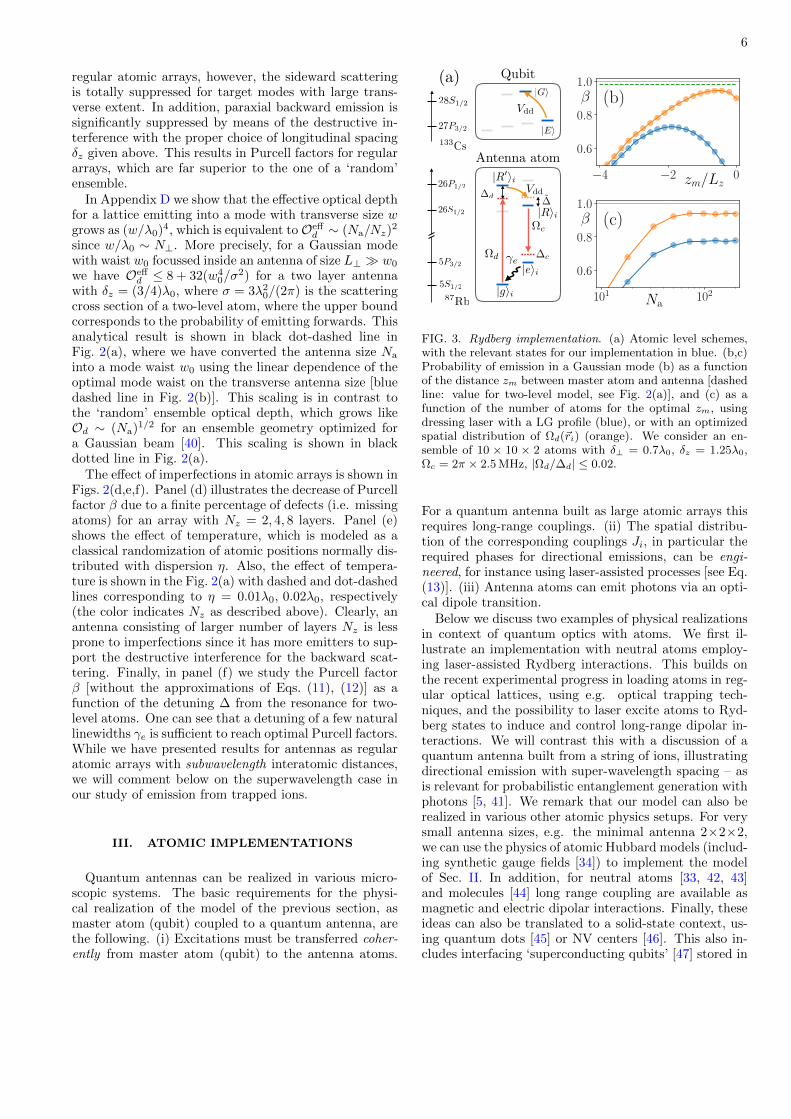
FIG. 3. Rydberg implementation. (a) Atomic level schemes,with the relevant states for our implementation in blue. (b,c)Probability of emission in a Gaussian mode (b) as a functionof the distance zm between master atom and antenna [dashedline: value for two-level model, see Fig. 2(a)], and (c) as afunction of the number of atoms for the optimal zm, usingdressing laser with a LG profile (blue), or with an optimizedspatial distribution of Ωd(~ri) (orange). We consider an en-semble of 10 × 10 × 2 atoms with δ⊥ = 0.7λ0, δz = 1.25λ0,Ωc = 2π × 2.5 MHz, |Ωd/∆d| ≤ 0.02.

For a quantum antenna built as large atomic arrays thisrequires long-range couplings. (ii) The spatial distribu-tion of the corresponding couplings Ji, in particular therequired phases for directional emissions, can be engi-neered, for instance using laser-assisted processes [see Eq.(13)]. (iii) Antenna atoms can emit photons via an opti-cal dipole transition.

Below we discuss two examples of physical realizationsin context of quantum optics with atoms. We first il-lustrate an implementation with neutral atoms employ-ing laser-assisted Rydberg interactions. This builds onthe recent experimental progress in loading atoms in reg-ular optical lattices, using e.g. optical trapping tech-niques, and the possibility to laser excite atoms to Ryd-berg states to induce and control long-range dipolar in-teractions. We will contrast this with a discussion of aquantum antenna built from a string of ions, illustratingdirectional emission with super-wavelength spacing – asis relevant for probabilistic entanglement generation withphotons [5, 41]. We remark that our model can also berealized in various other atomic physics setups. For verysmall antenna sizes, e.g. the minimal antenna 2×2×2,we can use the physics of atomic Hubbard models (includ-ing synthetic gauge fields [34]) to implement the modelof Sec. II. In addition, for neutral atoms [33, 42, 43]and molecules [44] long range coupling are available asmagnetic and electric dipolar interactions. Finally, theseideas can also be translated to a solid-state context, us-ing quantum dots [45] or NV centers [46]. This also in-cludes interfacing ‘superconducting qubits’ [47] stored in

7

strip line cavities with bilayer atomic ensembles actingas quantum antenna.

A. Rydberg Atoms

The atomic level structure we have in mind is shownin Fig. 3(a). For concreteness, we consider opticallytrapped atoms in a bilayer (Nz = 2) configuration, wherethe master atom is a 133Cs atom and the antenna ismade of 87Rb atoms. The state of the master atom isencoded in two Rydberg states |G〉 = |28S1/2,mj = 1

2 〉and |E〉 = |27P3/2,mj = 3

2 〉, with microwave transitionfrequency ωCs (the quantization axis is set by an externalmagnetic field along z). Antenna atoms can be excitedto four electronic levels, including two Rydberg states|R′〉i = |26P1/2,mj = − 1

2 〉 and |R〉i = |26S1/2,mj = 12 〉,

with transition frequency ωRb [48]. Our particular choiceof Rydberg states is motivated by the small energy differ-ence ∆ ≡ ωCs−ωRb = 2π×1.74(2) GHz between the twoRydberg transitions due to a Forster resonance [49]. Fi-nally, we choose two hyperfine stretched states, a groundstate |g〉i = |5S1/2, F = 2,mF = 2〉 and an excited state|e〉i = |5P3/2, F = 3,mF = 3〉, in order to generate opti-cal photons with λ0 = 780 nm (D2-line). In our model,we operate in the frozen gas regime [33], where the mo-tion of the atoms can be neglected for the timescalesassociated with our model.

While the complete atomic physics details are pre-sented in Appendix E, we describe here the main el-ements allowing this setup to behave as quantum an-tenna. First, the antenna atoms are subject to a laserbeam coupling off-resonantly, with spatial Rabi frequen-cies Ωd(~ri), and detuning ∆d, |g〉i to |R′〉i. In the dress-ing regime, Ωd(~ri), Vdd ∆d, where Vdd is the dipole-dipole coupling between Rydberg states (see Fig. 3),we obtain an effective coherent ‘flip-flop’ interaction|E〉 |g〉i → |G〉 |R〉i between master atom and antenna,which can be controlled externally via Ωd(~ri), i.e we canuse the dressing laser to write the required phases on theantenna atoms. Second, emission of optical photons from|Ri〉 is assisted by a control laser with Rabi frequenciesΩc(~ri), and detuning ∆c.

To show that good directionality can be achieved withrealistic configurations, we now present numerical sim-ulations showing the Purcell factor β for emission of asingle photon to a Gaussian mode, which include un-wanted dipole-dipole couplings between antenna atoms,and finite Rydberg states lifetimes. To complement thisanalysis, we also present in Appendix E a mapping toEq. (5), which is valid under the condition of the elec-tromagnetically induced transparency Ωc(~ri) Ji, γr,and ∆c = 0, with γr being the Rydberg decay rate. InFig. 3 (b,c) we show the Purcell factor β for the emissionto Gaussian modes. Panel (b) shows that an almost per-fect fidelity of coupling to a Gaussian target mode can bereached at a certain optimal qubit-antenna distance zm.The latter results from a tradeoff between an exagger-

−25 0 25 50z/λ0

−20

0

20x

λ0

1 2 4 6δz/λ0

1

3

5

7

βΘ

β(1)Θ

0.1

0.2

0.3

0.4

βΘ

5 10 15Na

2

4βΘ

(b)

FIG. 4. Ion string emission. (a) Electromagnetic field profile|~ϕ(~r )| (see text) for a chain of 10 ions as antenna with thelattice spacing δz = 3λ0, and numerically optimized couplingsJi. (b) Fraction of light βΘ emitted within a solid angle withΘ = π/8, as a function of lattice spacing δz. The couplingsJi are given by (green) plane wave eik0zi , (orange) optimalGaussian phase profile, and (blue) unconstrained optimizedcouplings. Inset: βΘ as a function of Na for δz = 3λ0 (solid),4λ0 (dashed), 5λ0 (dot-dashed).

ated inhomogeneity of the dipole-dipole couplings Ji atsmall zm and the predominance of unwanted losses fromthe Rydberg states at large zm. In panel (c) we showthat the effect of inhomogeneity can be significantly mit-igated by using an optimized spatial distribution of Rabifrequencies Ωd(~ri) (instead of LG mode). This showsthat the atomic antenna based on Rydberg atoms can berealized with state-of-art technology and with realisticparameters.

B. Trapped Ions

We considered above 3D geometries with sub-wavelength separations, allowing for an almost perfectmode-matching to a given photonic mode. We show be-low that even in 1D atomic strings with super-wavelengthspacings δz > λ0 [50–53] directional emission can beachieved. This is of interest for trapped ions setups [54–57], in particular to implement probabilistic protocolswith high repetition rates.

We consider a model system of trapped ions as a 1Dchain with fixed separation δz (N⊥ = 1), with the firstion implementing the master atom (qubit), while the restof the chain represents the antenna. We assume herethat we can implement the coupling Hamiltonian H0A

with arbitrary couplings Ji, using for instance a digitalapproach based on a universal set of gates. We show inFig. 4(a) the spatial profile obtained for a chain of 10 ionsas antenna. The photonic mode is clearly directional,with a significant fraction of light emitted within an apexangle of 2Θ = π/4, which can then be collected with anoptical lens.

To quantify directionality of the optical emission, wedefine

βΘ ≡ limr→∞

1

A

∫ Θ

0

sin θdθ

∫ 2π

0

dφ |~ϕ (r, θ, φ)|2 , (14)

corresponding to the amount of radiation emitted within

8

a solid angle of a cone with an apex angle 2Θ. The in-tegral is evaluated in spherical coordinates with respectto the chain axis, and the normalization coefficient is

defined as A ≡∫ π

0sin θdθ

∫ 2π

0dφ |~ϕ (r, θ, φ)|2. We show

in Fig. 4(b) the value of βΘ/β(1)Θ for different configura-

tions of the couplings Ji, where β(1)Θ corresponds to the

case of single ion emission. Significant improvement canbe achieved even for super-wavelength spacings δz > λ0.Note that choosing the Ji according to a Gaussian profileinstead of plane wave, provides nearly optimal direction-ality.

IV. OUTLOOK

We have proposed a model for a directional atom-lightinterface with few atoms. While we focused here on emis-sion properties, quantum antennas can also be used toabsorb photons from a particular mode. In analogy tochiral quantum optics in 1D, where atoms coupled tooptical nanostructures emit and absorb photons propa-gating in a single direction, we can thus achieve ‘chi-rality in 3D’. In particular, an array of master atomscan be coupled to the same directional mode, thereby

forming a cascaded system. This can be directly appliedto build quantum networks in free space, where severalmaster atoms — each equipped with a quantum antenna— interact by exchanging photons. In such network,the connectivity can be modified dynamically, allowingfor faithful quantum communication [58], e.g. to realizequantum state transfer [59], deterministically or proba-bilistically, between distant quantum computers. Thisgeneralizes to the transfer of more complex states, build-ing on the quantum nature of the antenna, which couldbe used to emit for example quantum error correctingphotonic codes [60], rather than single photons.

ACKNOWLEDGMENTS

We thank R. Blatt, T. Monz, M. Saffman, M. Lukinand J. I. Cirac for discussions. The parameters for theRydberg simulations were obtained using the ARC li-brary [61]. This work was supported by the Army Re-search Laboratory Center for Distributed Quantum In-formation via the project SciNet, the ERC Synergy GrantUQUAM and the SFB FoQuS (FWF Project No. F4016-N23).

[1] B. R. Mollow, Physical Review 188, 1969 (1969).[2] H. J. Kimble, Nature 453, 1023 (2008).[3] T. E. Northup and R. Blatt, Nature Photonics 8, 356

(2014).[4] M. K. Tey, Z. Chen, S. A. Aljunid, B. Chng, F. Huber,

G. Maslennikov, and C. Kurtsiefer, Nature Physics 4,924 (2008).

[5] L.-M. Duan and C. Monroe, Reviews of Modern Physics82, 1209 (2010).

[6] N. Trautmann, G. Alber, G. S. Agarwal, and G. Leuchs,Physical Review Letters 114, 1 (2015).

[7] K. M. Birnbaum, A. Boca, R. Miller, A. D. Boozer, T. E.Northup, and H. J. Kimble, Nature 436, 87 (2005).

[8] F. Haas, J. Volz, R. Gehr, J. Reichel, and J. Esteve,Science 344, 180 LP (2014).

[9] A. Reiserer and G. Rempe, Reviews of Modern Physics87, 1379 (2015).

[10] R. McConnell, H. Zhang, J. Hu, S. Cuk, and V. Vuletic,Nature 519, 439 (2015).

[11] T. G. Tiecke, J. D. Thompson, N. P. De Leon, L. R. Liu,V. Vuletic, and M. D. Lukin, Nature 508, 241 (2014).

[12] J. D. Hood, A. Goban, A. Asenjo-Garcia, M. Lu, S.-P.Yu, D. E. Chang, and H. J. Kimble, Proceedings of theNational Academy of Sciences 113, 10507 LP (2016).

[13] R. J. Coles, D. M. Price, J. E. Dixon, B. Royall,E. Clarke, P. Kok, M. S. Skolnick, A. M. Fox, and M. N.Makhonin, Nature Communications 7, 11183 (2016).

[14] N. V. Corzo, B. Gouraud, A. Chandra, A. Goban, A. S.Sheremet, D. V. Kupriyanov, and J. Laurat, PhysicalReview Letters 117, 133603 (2016).

[15] P. Solano, P. Barberis-Blostein, F. K. Fatemi, L. A.Orozco, and S. L. Rolston, Nature Communications 8,

1 (2017).[16] P. Lodahl, S. Mahmoodian, S. Stobbe, A. Rauschenbeu-

tel, P. Schneeweiss, J. Volz, H. Pichler, and P. Zoller,Nature 541, 473 (2017).

[17] R. J. Bettles, S. A. Gardiner, and C. S. Adams, PhysicalReview Letters 116, 103602 (2016).

[18] E. Shahmoon, D. S. Wild, M. D. Lukin, and S. F. Yelin,Physical Review Letters 118, 113601 (2017).

[19] A. Asenjo-Garcia, M. Moreno-Cardoner, A. Albrecht,H. J. Kimble, and D. E. Chang, Physical Review X 7,31024 (2017).

[20] M. T. Manzoni, M. Moreno-Cardoner, A. Asenjo-Garcia,J. V. Porto, A. V. Gorshkov, and D. E. Chang,arXiv:1710.06312.

[21] J. Perczel, J. Borregaard, D. Chang, H. Pichler, S. Yelin,P. Zoller, and M. Lukin, Physical Review Letters 119,23603 (2017).

[22] S. He, Y. Cui, Y. Ye, P. Zhang, and Y. Jin, MaterialsToday 12, 16 (2009).

[23] J. Sun, E. Timurdogan, A. Yaacobi, E. S. Hosseini, andM. R. Watts, Nature 493, 195 EP (2013).

[24] I. Bloch, J. Dalibard, and S. Nascimbene, Nature Physics8, 267 (2012).

[25] B. J. Lester, N. Luick, A. M. Kaufman, C. M. Reynolds,and C. A. Regal, Physical Review Letters 115, 73003(2015).

[26] T. Xia, M. Lichtman, K. Maller, A. W. Carr, M. J. Pi-otrowicz, L. Isenhower, and M. Saffman, Physical Re-view Letters 114, 1 (2015).

[27] M. Endres, H. Bernien, A. Keesling, H. Levine, E. R.Anschuetz, A. Krajenbrink, C. Senko, V. Vuletic,M. Greiner, and M. D. Lukin, Science 354, 1024 (2016).

9

[28] D. Barredo, S. de Leseleuc, V. Lienhard, T. Lahaye, andA. Browaeys, Science 354, 1021 LP (2016).

[29] M. Saffman and T. G. Walker, Physical Review A 66,65403 (2002).

[30] M. Saffman and T. G. Walker, Physical Review A -Atomic, Molecular, and Optical Physics 72, 1 (2005).

[31] M. O. Scully, E. S. Fry, C. H. R. Ooi, and K. Wodkiewicz,Physical Review Letters 96, 10501 (2006).

[32] M. Saffman, T. G. Walker, and K. Mølmer, Reviews ofModern Physics 82, 2313 (2010).

[33] A. Browaeys, D. Barredo, and T. Lahaye, Journal ofPhysics B: Atomic, Molecular and Optical Physics 49(2016).

[34] N. Goldman, J. C. Budich, and P. Zoller, Nature Physics12, 639 (2016).

[35] R. H. Lehmberg, Physical Review A 2, 883 (1970).[36] D. F. V. James, Physical Review A 47, 1336 (1993).[37] K. Hammerer, A. S. Sørensen, and E. S. Polzik, Reviews

of Modern Physics 82, 1041 (2010).[38] A. V. Gorshkov, A. Andre, M. D. Lukin, and A. S.

Sørensen, Phys. Rev. A 76, 33805 (2007).[39] Such modes can be further transformed by optical lenses

to interface the master atom with another system of in-terest, such as an optical fiber, a nanophotonic device,an extra master atom, etc.

[40] The optimal overlap with a Gaussian beam is achievedfor an ensemble of length 2zR ≡ 2πw2

0/λ0 (i.e. twice theRayleigh length) and section S = πw2

0. This ensemblecontains Na = 2naSzR = 2naS

2/λ0 atoms, such that

Od ≡ (σ/S)Na = σ(2naNa/λ0)1/2 with σ the resonantscattering cross section of a two-level atom.

[41] C. Cabrillo, J. I. Cirac, P. Garcıa-Fernandez, andP. Zoller, Phys. Rev. A 59, 1025 (1999).

[42] T. Lahaye, C. Menotti, L. Santos, M. Lewenstein, andT. Pfau, Reports Prog. Phys. 72, 126401 (2009).

[43] A. W. Glaetzle, K. Ender, D. S. Wild, S. Choi, H. Pichler,M. D. Lukin, and P. Zoller, Physical Review X 7, 31049(2017).

[44] A. Micheli, G. K. Brennen, and P. Zoller, Nat. Phys. 2,341 (2006).

[45] P. Lodahl, S. Mahmoodian, and S. Stobbe, Reviews ofModern Physics 87, 347 (2015).

[46] J. Cai, A. Retzker, F. Jelezko, and M. B. Plenio, Nat.Phys. 9, 168 (2013).

[47] A. a. Houck, H. E. Tureci, and J. Koch, Nat. Phys. 8,292 (2012).

[48] The nuclear spin mI = 3/2 can be considered as specta-tor due to the small hyperfine interactions between Ry-dberg levels.

[49] T. Walker and M. Saffman, Phys. Rev. A 77, 32723(2008).

[50] G. Y. Slepyan and A. Boag, Physical Review Letters 111,1 (2013).

[51] R. Wiegner, S. Oppel, D. Bhatti, J. Von Zanthier, andG. S. Agarwal, Physical Review A - Atomic, Molecular,and Optical Physics 92, 1 (2015).

[52] D. Bhatti, S. Oppel, R. Wiegner, G. S. Agarwal, andJ. von Zanthier, 013810, 1 (2016).

[53] J. Liu, M. Zhou, L. Ying, X. Chen, and Z. Yu, PhysicalReview A 95, 1 (2017).

[54] M. Harlander, R. Lechner, M. Brownnutt, R. Blatt, andW. Hansel, Nature 471, 200 (2011).

[55] C. Monroe and J. Kim, Science 339, 1164 LP (2013).

[56] N. H. Nickerson, J. F. Fitzsimons, and S. C. Benjamin,Physical Review X 4, 41041 (2014).

[57] C. Senko, P. Richerme, J. Smith, A. Lee, I. Cohen,A. Retzker, and C. Monroe, Physical Review X 5, 21026(2015).

[58] N. Sangouard, C. Simon, H. de Riedmatten, andN. Gisin, Reviews of Modern Physics 83, 33 (2011).

[59] J. I. Cirac, P. Zoller, H. J. Kimble, and H. Mabuchi,Physical Review Letters 78, 3221 (1997).

[60] M. H. Michael, M. Silveri, R. T. Brierley, V. V. Albert,J. Salmilehto, L. Jiang, and S. M. Girvin, Physical Re-view X 6, 031006 (2016).

[61] N. Sibalic, J. D. Pritchard, C. S. Adams, and K. J.Weatherill, Computer Physics Communications 220, 319(2017).

Appendix A: Properties of Laguerre-Gauss beams

Here we summarize notation, properties andparametrization of Laguerre-Gauss (LG) modesas used repeatedly in the main text. LG modesare particular solutions of the paraxial equation(∂z − i

2k0∇2⊥

)LGlp (~ρ, z) = 0, and are defined, for a

given optical wavelength λ0, by the mode waist w0 [seeFig. 1] as

LGlp (~ρ, z) =

√2p!

π(p+ |l|)!1

w(z)

(ρ√

2

w(z)

)|l|e− ρ2

w2(z)

L|l|p

(2ρ2

w2(z)

)ei

k0ρ2

2R(z)+ilφ+iξ(z),

(A1)

where ρ ≡ |~ρ| and φ = atan(y/x), which defines a

basis with∫d2ρup,l (~ρ, z)

(up′,l′ (~ρ, z)

)∗= δl,l′δp,p′ . For

simplicity we assume here that the origin for z is lo-

cated at the waist. Here L|l|p denotes the generalized

Laguerre polynomials, where the radial index p ≥ 0 andthe azimuthal index l are integers. The curvature ra-dius is defined as R (z) = z + z2

R/z, and the Gouy phaseas ξ(z) = tan−1(z/zR), with zR the Rayleigh lengthzR ≡ πw2

0/λ0. The mode width at position z is expressed

as w(z) ≡ w0

√1 + z2/z2

R.

Appendix B: Emission rate into paraxial mode

In this section we derive Eq. (9) of Sec. II B for theemission rates γn to a set of orthogonal paraxial modesun (~ρ, z). The photon flux into these modes is definedthrough the overlap of the emitted field with the corre-sponding modes, in a plane transverse to the propagationaxis z, and located at zp λ0 to neglect the near-fieldeffects. This allows us to identify

γn = c

∣∣∣∣∫ d2~ρ u∗n(~ρ, zp)~p∗~ϕ(~r )

∣∣∣∣2 .

10

Taking zp far enough from the antenna, only the paraxialpart of ϕ(~r ) will contribute, and we can replace the Greenfunction in Eq. (8) by its paraxial counterpart as

~p ∗G(~r − ~ri)~p→3πk−20 Gpar(~ρ− ~ρi, z − zi)

=3πk−20

∑n

eik0(z−zi)un(~ρ, z)u∗n(~ρi, zi).

(B1)

Here we have definedGpar(~ρ, z) = k0eik0[z+|~ρ|2/(2z)]/(2iπz)

with the property∫d2~ρ u∗n(~ρ, zp)Gpar(~ρ− ~ρi, zp − zi) = u∗n(~ρi, zi). (B2)

This gives Eq. (9) of the main text.

Appendix C: Purcell factor for atomic ensemblewith random atomic positions

In this Section we derive analytically an expression ofPurcell factors for an ensemble of Na atoms, as quotedin Sec. II B, with atoms randomly distributed in a boxwith volume V = L2

⊥ ×Lz. We start from Eqs. (11) and(12) in the limit of large detuning ∆→∞ and write

βn =1

~J† [I + Re(G)] ~J

3π

2k20

∣∣∣∣∣∑i

u∗n (~ρi, zi) e−ik0ziJi

∣∣∣∣∣2

,

(C1)

where, for convenience, we use the vector notation ~J ≡J1, . . . JN. From Eq. (B1) we have for the term indenominator

~J†Re(G) ~J ≈ 3π

2k20

∑n

∣∣∣∣∣∑i

u∗n (~ρi, zi) e−ik0ziJi

∣∣∣∣∣2

Substituting this expression in Eq. (C1) we get

βn =σ4

∣∣∑i u∗n (~ρi, zi) e

−ik0ziJi∣∣2

~J† ~J + σ4

∑m |∑i u∗m (~ρi, zi) e−ik0ziJi|2

, (C2)

where we defined the single atom resonant scatteringcross-section as σ ≡ 3λ2

0/(2π) = 6π/k20. Let us as-

sume now that the coefficients Ji are chosen in or-der to maximize the emission to the mode un0

asJi ∼ eik0ziun0

(ρi, zi). Assuming the transverse size ofthe atomic cloud is larger than the mode waist, i.e.w0 . L⊥, and transforming the sum in Eq. (C2) to anintegral

∑i → na

∫Vd3r, we get

βn0=

σ4 |naLz|2

naLz + σ4 |naLz|2

≡ Od4 +Od

,

with the optical depth defined as Od ≡ σnaLz.

Appendix D: Optical depth of a 3D lattice

In this Section we derive an analytical expression forthe Purcell factor and the effective optical depth for atwo layer phased array of emitters, as quoted in Sec-tion II C. Here we consider arrays infinite in the trans-verse directions, and we neglect polarization effects. Thelattice spacings in the longitudinal and transverse di-rections are δz and δ⊥, respectively. The array is pre-pared to emit a photon unidirectionally with wavevec-tor k0 into a mode with transverse spatial distribu-tion f(~ρ ) of a large width w λ0 with λ0 the pho-ton wavelength. Therefore, the mode transverse spatialspectrum F⊥(~q ) =

∫f(~ρ )e−i~q~ρd~ρ has a narrow width

qmax ∼ 1/w k0.

The unnormalized probability amplitude ϕ(~q, kz) to

emit a photon into a plane wave with wavevector ~k =~q, kz can be found as the limit |~r | → ∞ of the Eq. (8)

in the main text, for ~r = |~r |(~k/|~k |). Here we neglect thepolarization part of the Green’s function and considerthe limit of large detunings ∆ γe. For a two layerarray of emitters (located at z = ±δz/2) with the phasesfixed, according to the prescription (13) (in the maintext), to emit light into the transversally wide mode, i.e.Jj = eik0zjf(~ρj), the probability amplitude ϕ(~q, kz) reads

ϕ(~q, kz) =∑j

Jje−i~q ~ρj−ikzzj

=[e−i(k0−kz)δz/2 + ei(k0−kz)δz/2

]×∑k,l

f(δ⊥k, δ⊥l)e−i(qxδ⊥k+qyδ⊥l)

∼[e−i(k0−kz)δz/2 + ei(k0−kz)δz/2

]F⊥(~q ).

Here the approximation of the sum with the continu-ous function F⊥(~q ) becomes exact for a lattice spacingδ⊥ < (2qmax)−1, according to the sampling theorem. Theensemble does not emit in the transverse direction, as thespectrum F⊥(~q ) goes to zero for qx,y > qmax. Thus thephoton can be emitted into paraxial forward and back-ward modes only.

In order to define the Purcell factor we need to find thecorresponding amplitudes to emit photon forward andbackward. First, we consider emission into the parax-ial backward modes with k←z ≈ −k0 + (q2

x + q2y)/(2k0).

The longitudinal spacing δz is chosen to suppress the ex-act backward scattering (given by the plane wave withkz = −k0, qx,y = 0), i.e. δz = λ0(2Nz − 1)/(2Nz). Thebackward scattering amplitude for the interlayer spacing

11

δz = (3/4)λ0 reads

ϕ←(~q ) =[e−i(k0−k

←z )δz/2 + ei(k0−k

←z )δz/2

]F⊥(~q )

≈ −2 sin

[3π

8

(q2x + q2

y)

k20

]F⊥(~q )

≈ q2x + q2

y

k20

F⊥(~q ).

The probability to emit light backward is proportional to∫d~q |ϕ←(~q)|2, and is given by

P← ∼∫dqxk0

dqyk0

∣∣∣∣∣q2x + q2

y

k20

F⊥(qx, qy)

∣∣∣∣∣2

≈ 1

2

∫ qmax

0

dq2r

k20

(q2r

k20

)2

=1

6

(qmax

k0

)6

∼(λ0

w

)6

.

Here we approximated the spectrum function as a con-stant for q2

x + q2y ≤ q2

max and zero otherwise. On theother hand, the forward scattering amplitude has a lead-ing term of order 1, and the probability to emit forwardreads

P→ ∼∫dqxk0

dqyk0|F⊥(q)|2

≈ 1

2

∫ qmax

0

dq2r

k20

1

=1

2

(qmax

k0

)2

∼(λ0

w

)2

.

The Purcell factor is thus given by βΘ = P→/(P→+P←)with Θ = π/2 as defined in (14) of the main text. Thisallows us to read off the effective optical depth for a twoinfinite layers emitting into a transversally confined modeas

Oeffd (Θ) ≡ 4βΘ

1− βΘ=

4P→P←

∼(w

λ0

)4

.

The effective optical depth for emission into a Gaussianmode as used in the main text is bounded above by theexpression Oeff

d ≤ Oeffd (π/2). This is the result quoted in

Section II C.More precisely, for a two-layer antenna with phases

chosen to emit into a Gaussian mode with a beam waistw0,

Jj ∼ eik0zjLG00(~ρj , zj),

as discussed in Section II C, one can show that the effec-tive optical depth for forward emission (within the solidangle with Θ = π/2) reads

Oeffd (π/2) = 8 + 32(w4

0/σ2),

where σ = 3λ20/(2π) is the scattering cross section of a

two-level atom and the calculation is performed for theinterlayer spacing δz = (3/4)λ0.

Appendix E: Details of the Rydberg implementation

In this Section we provide details on our Rydberg im-plementation discussed in Sec. III.

1. Model

In a frame rotating with the laser frequencies, thequantum-optical Hamiltonian describing our model canbe written in the formHRyd = H0A+HAF+H0F+Hlosses,where we have

H0A = −∑i

[(∆d + ∆) |R〉i 〈R|

+ ∆d |R′〉i 〈R′|+ ∆c |e〉i 〈e|]

+∑i

[Ωd(~ri) |g〉i 〈R′|+ Ωc(~ri) |R〉i 〈e|+ h.c.]

+∑i

Vdd(~ri − ~rm) (|ER′i〉 〈GRi|+ h.c)

+∑i<j

V ′dd(~ri − ~rj)(|RjR′i〉 〈R′jRi|+ h.c

),

with Vdd(~ri − ~rm) = C3(1− 3 cos2 θi,m)/r3i,m the desired

‘flip-flop’ process transferring excitations between mas-ter atom and antenna atoms, and where V ′dd(~ri − ~rj) =C ′3(1 − 3 cos2 θij)/r

3i,j describes dipole-dipole couplings

between antenna atoms. Here, ~rm is the position ofthe master atom, rab = |~ra − ~rb|, and cos θab = [(~ra −~rb) · ~z ]/rab. For the levels chosen above, we have C3 ≈49.3hMHzµm3, C ′3 ≈ 41.5hMHzµm3. The Hamilto-nians HAF and H0F are introduced in the main text.Finally, we model in a first approximation the natural de-cay of the Rydberg states with a non-Hermitian Hamilto-nian Hlosses = −i(γr/2) (|R〉i 〈R|+ |E〉i 〈E|), with γr =2π × 3.6 KHz.

2. Perturbative regime

By choosing ∆d + ∆ = 0, and in the regime Ωd, Vdd ∆d, we can eliminate in second-order perturbation theorythe state |R′〉i and obtain

H0A =∑i

Ji (|Egi〉 〈GRi|+ h.c)

+∑i<j

J ′ij (|Rjgi〉 〈gjRi|+ h.c)

+∑i

[Ωc(~ri) |R〉i 〈e|+ h.c.]−∆c |e〉i 〈e| , (E1)

allowing long-range coherent excitation transfer frommaster atom to antenna atoms. Here the ‘dressed’ cou-plings Ji = Vdd(~ri−~rm)Ωd(~ri)/∆d can be engineered viathe dressing-laser Rabi frequency Ωd(~ri). Note that we

12

did not write the additional AC Stark shifts contribu-tions, which can be included in the definitions of the de-tunings (or compensated via additional laser couplings).

Note that our effective Hamiltonian (E1) is not identi-cal to the model presented in the main text [see Eq. (2)].First, instead of two level atoms with detunings ∆, weobtain here an antenna built from three-level atoms,where the decay from Rydberg to ground state is Ra-man assisted by the control laser Ωc(~ri). Second, exci-tations can also hop between antenna atoms with J ′ij =

V ′dd(~ri − ~rj)Ωd(~ri)Ω∗d(~rj)/∆2d.

3. Study of three-level atoms antennas

To assess the performance of three-level antennas, wecalculate numerically the spatial profile of the mode ~ϕ(~r )generated via the excitation transfer to the antenna, asgoverned by Eq. (E1). We can also obtain an analyticalexpression for the decay rate γtot and for ~ϕ(~r ). Assuming∆c = 0 and a strong control field Ωc Ji, J

′i,j , γr, we

obtain Eqs. (11), (12) with the identification Ji/∆ →Ji/Ωc (~ri). In this limit, we establish a direct connectionbetween our Rydberg implementation and our model oftwo-level antenna presented in the main text.