a feasibility study for reset control of an industrial
TRANSCRIPT

A FEASIBILITY STUDY FOR RESET CONTROL OF AN INDUSTRIAL BATCH REACTOR
By Roanne Lahee
BSc. Eng. (Chem.) (University of the Witwatersrand)
A dissertation submitted in partial fulfilment of the requirements for the degree of
MASTER OF SCIENCE IN ENGINEERING
IN THE DEPARTMENT OF CHEMICAL ENGINEERING
UNIVERSITY OF CAPE TOWN
March 2010
Supervisor: Prof. Martin Braae
DEPARTMENT OF ELECTRICAL ENGINEERING UNIVERSITY OF CAPE TOWN

ii
ABSTRACT
A feasibility study for the application of reset control to the temperature control loop of a
pressurized exothermic batch leach reactor in the hydrometallurgical Precious Group Metals
(PGM) industry is carried out in this dissertation.
The industrial reactor needs tight control to maximize the dissolution of PGM’s and to minimize
batch time. Historically, the temperature in the reactor has been observed to oscillate excessively
with large overshoots, especially during start-up. Severe temperature overshoot could potentially
lead to reaction runaway, which has serious safety implications.
The literature indicates that a reset controller is a linear system that “resets” some or all of its
states to zero when its input is zero, based on a given reset law. The theory holds that reset
controllers have the ability to dramatically decrease overshoot and settling time without sacrificing
rise time, hence the potential for application to the particular reactor temperature control loop.
Since the theory of reset control requires application to an optimised control system, an in-depth
control analysis was performed on the existing operation in order to develop a fundamental
understanding of the process with a view to improving its control, operability and performance
efficiency. The investigation identified an array of practical control problems, many of which had
to be addressed first in order to quantify the benefits that would result from implementation of a
reset controller in this industrial reactor process.
The improvement in plant performance associated with progressing from the plant in its initial
condition to the plant once its existing control had been fixed and optimized to the plant operating
under reset control is demonstrated in the dissertation. A number of different graphical
techniques were developed using MATLAB in order to visualize and analyse the relevant data
before and after implementation of control changes on the existing control solution.
After optimization of the existing control solution, the industrial reactor temperature response to
cooling was modelled and simulated using MATLAB and SIMULINK software packages. These
simulations are used to draw a direct comparison between the existing PI controller, an optimized
linear PI controller, an optimized linear PI controller with lead, and a reset controller. The
simulations confirm the ability of reset control to significantly reduce temperature overshoot as
well as decrease the settling time in this industrial process control loop. The simulations also
highlight some typical practical issues, including the effects of dead time and noise, which are
critical in the application of theoretical control solutions in an industrial environment.

iii
In applying the modern theory of reset control to the industrial reactor the predominant theory was
found to assume a restrictive dynamic model for the plant; one in which the input has to be zero
to keep the output constant at a non-zero value. In other cases the theory of reset control
assumed that the plant input could be set to zero on reset, and this was not allowed for on the
industrial plant.
In the dissertation these limitations of the basic theory were addressed by modifying the reset
controller to enable its application on this particular industrial process. In the literature actual
industrial applications of reset control appear to be scarce, and the incorporation of a non-zero
initial condition for a reset controller may well be unique.
Keywords: Reset control; Clegg integrator; initial states; industrial batch reactor; temperature
control; exothermic reactions; multiple reactions; dissolve; leach; hydrometallurgy;
platinum; Precious Group Metals (PGMs).

iv
DECLARATION I declare that this dissertation, submitted for the degree of Master in Science in Engineering at the
University of Cape Town, has not been submitted prior to this for any degree or examination, at
this or any other university.
I know the meaning of plagiarism and declare that all the work in the document, save for that
which is properly acknowledged, is my own.
____________________
Roanne Lahee
March 2010

v
ACKNOWLEDGEMENTS My sincere thanks goes to all those involved in this project in various ways. More specifically to
the following people and institutions:
• Anglo Platinum – for full financial sponsorship of the project.
• Prof. Martin Braae (Department of Electrical Engineering, UCT) – MSc supervisor.
• Leon Coetzer (Head of Process Control Department, Anglo Platinum) – candidate’s manager
during MSc.
• Nic Lombard (Anglo Platinum Process Control Department) – input into regulatory analysis.
• Dev Groenewald (Anglo Platinum Process Control Department) – input into data visualization
techniques.
• PMR Production & Instrumentation, Deryck Spann (PMR Head of Operations, Anglo
Platinum).
• Peter Charlesworth (Anglo Platinum consultant) & Richard Grant (Johnson Matthey
Technology consultant) – involved in original development of the industrial batch reactor
process, and responsible for internal PGM Chemistry Refining Course.
• Prof. Mike Nicol & Prof. Peter Gaylard (Department of Chemical Engineering, UCT) –
responsible for MSc coursework.
• Neville Plint (Head of Research & Development, Anglo Platinum), Les Bryson (Manager
Refining Technology, Anglo Platinum) and Lloyd Nelson (Head of Smelting & Refining
Technology, Anglo Platinum) – support.

vi
TABLE OF CONTENTS ABSTRACT DECLARATION ACKNOWLEDGEMENTS TABLE OF CONTENTS LIST OF ABBREVIATIONS 1. INTRODUCTION………………………………………………………………1 2. LITERATURE REVIEW………………………………………………………6
2.1. Overview……………………………………………….………………6 2.2. Industrial Batch Reactor Process Description……………….…7
2.2.1. Process Background, Chemistry and Design Parameters……...7
2.2.2. Existing Equipment…………………………………………………17
2.2.3. Batch Process Phases……………………………………………..20
2.2.4. Multivariable System………………………………………………..23
2.2.5. Importance of Accurate Temperature Control…………………...30
2.3. Reset Control……………………….………………………………...34 2.3.1. Theory………………………………………………………………...35
2.3.2. History and Development…………………………………………..41

vii
3. CONTROL STUDY AND OPTIMIZATION OF EXISTING SYSTEM….…55 3.1. Control Study Method…….…………………………………………55 3.2. Existing Control Solution, Measurements and
Manipulated Variables………………………...…...………………..59 3.3. Existing Control Performance Analysis and Optimization…...63
3.3.1. Typical Batch Operation…………………………………………….63
3.3.2. Temperature Control………………………………………………...64
3.3.3. Chlorine Flow Control………………………………………………..66
3.3.4. Regulatory Control…………………………………………………...68
3.3.5. Performance Monitoring……………………………………………..68
4. SYSTEM IDENTIFICATION AND PROCESS MODEL ANALYSIS….….70
4.1. Step Tests……………………………………………..………………70 4.2. Dynamic Process Modelling………………………………………..71
5. CONTROLLER DESIGN AND COMPARISON BY SIMULATION………73
5.1. Process Control Loop Simulation Model………………………...73
5.1.1. Model Overview………………………………………………………73
5.1.2. Independent Gains Equation………………………………………..76
5.1.3. Loop Update Time and PLC Scan Rate………………………...…79
5.1.4. Engineering Scaling Factors………………………………………..80
5.1.5. Valve Saturation……………………………………………………...80
5.2. Existing PI Controller Base Case Simulation………………...…81 5.2.1. Control Loop Analysis……………………………………………….81
5.2.2. Closed Loop Simulation……………………………………………..84
5.3. PI Controller Design and Modelling………………………………89 5.3.1. Control Loop Optimization…………………………………………..89
5.3.2. Control Loop Analysis……………………………………………….99
5.3.3. Closed Loop Simulation……………………………………..…..…102

viii
5.4. PID Controller Design and Modelling…………………………...104 5.4.1. Control Loop Optimization………………………………………....104
5.4.2. Control Loop Analysis………………………………………………107
5.4.3. Closed Loop Simulation……………………………………………110
5.5. Reset Controller Design and Modelling……………………...…113 5.5.1. Reset Controller Solution……………………………………….....113
5.5.2. Non-zero Initial Conditions for Reset Control……………………115
5.5.3. Reset Controller Sensitivity to Dead Time……………………….120
5.5.4. Reset Controller Sensitivity to Noise Disturbances……………..123
5.6. Controller Comparison and Evaluation by Simulation………123 6. CONCLUSION & RECOMMENDATIONS………………………………...125 LIST OF REFERENCES…………………………………………………………….128 APPENDIX
Appendix 1: Other SIMULINK Models Investigated During the Design and Simulation of
the Improved PID or Linear PI with Lead Controller
Appendix 2: Other SIMULINK Models Investigated During the Design and Simulation of
the Reset Controller
Appendix 3: Temperature-Cooling Control Loop Simulation Model (SIMULINK)

ix
LIST OF ABBREVIATIONS
PGM - Platinum Group Metal
PSS - Platinum Salt Sensitivity
MPC - Model Predictive Control
MSPC - Multivariate Statistical Process Control
EMs - Engineering Modules
CMs - Control Modules
PLC - Programmable Logic Controller
PI - Proportional-Integral
PID - Proportional-Integral-Derivative
Pt - Platinum
Pd - Palladium
Rh - Rhodium
Ir - Iridium
Ru - Ruthenium
Au - Gold
Cl - Chlorine
HCl - Hydrochloric Acid
S - Sulphur
Si - Silica
T - Temperature
P - Pressure
F - Flowrate
JMTC - Johnson Matthey Technology Centre (U.K.)
PID - Proportional-Integral-Derivative
GLV - Glass-lined vessel
HAZOP - Hazard and Operability study
ST - Steam
CW - Cooling Water
CL - Chlorine Gas
FORE - First Order Reset Element
LTI - Linear Time-invariant
FORE - First Order Reset Element
IDE - Impulsive Differential Equation
BIBO - Bounded-Input Bounded-Output
UBIBS - Uniform Bounded-Input Bounded-State
IQC - Integral Quadratic Constraint

1
1. INTRODUCTION This dissertation is essentially a detailed control study of a pressurized exothermic batch reactor
in the hydrometallurgical Precious Group Metals (PGM) industry.
The industrial batch reactor process – which is the crucial first step in the hydrometallurgical
precious metal refining flowsheet – involves an acid leach where a range of PGM and base
metals present in the solid feed are dissolved into solution through aggressive chloride attack.
Once the metals are in solution, this renders them amenable to further sequential
hydrometallurgical separation downstream. Therefore the efficiency of this reactor dissolve stage
is critical to the performance of the entire precious metals refinery.
The primary dissolve (or leach) process is carried out under conditions of elevated temperature
and pressure, which have been optimized under laboratory conditions to maximize the rate of
metal dissolution and thereby minimize batch time. These specific operating conditions are also
designed to maximize impurity removal in the process upfront, and in so doing achieve the
condition of dissolve liquor required for subsequent chemical processing downstream. Therefore
accurate control of temperature and pressure is important in achieving the original design
objectives, and to improve the process efficiency.
More importantly, however, the use of chlorine and hydrochloric acid under these high
temperature and pressure conditions, and in the presence of highly exothermic reactions with the
potential of runaway constitutes a critical safety risk. Conditions of poor control could well lead to
hazardous chlorine leaks or volatile reactor spillage of hot hydrochloric acid liquors, both cases
requiring the immediate evacuation of operating personnel from the process area to prohibit
permanent corrosive chemical damage to tissues of the lungs, eyes and skin. In addition the
dissolved process liquor itself can potentially contain certain metal species in a form which can
have various serious health side effects, including PSS (platinum salt sensitivity or platinosis) and
hence must be contained in the sealed reactor at all times with spillages avoided at all costs.
All these factors together present an important and unique control challenge for this specific
industrial reactor. In addition, the batch reactor process can be broken into a number of distinct
sequential phases where the reactor control performance and requirements are complicated by
the fact that the chemistry, exothermicity and dynamics of these sequential phases differ
dramatically from one another as the batch proceeds with time.

2
During Phase I steam is supplied in order to provide the necessary activation energy needed to
kick-start the PGM dissolution reactions. During Phase II the “alloy” particles containing the
majority of the PGM’s are dissolved and the majority of the chlorine consumption occurs. The
chlorine reacts as fast as it can dissolve into the liquid phase so the rate of dissolution is mass
transfer limiting. The reactions are also highly exothermic and must be limited according to the
available cooling capacity in order to prevent temperature and pressure runaway. Phase III
occurs as the initial dissolution reactions reach completion and the chlorine concentration in
solution builds up causing a rise in redox, which allows certain of the other metals to dissolve.
During Phase IV the solution is totally saturated with chlorine and only residual values of PGM’s
remain undissolved. The rate determining step is now chemical reaction limiting and in order to
maintain the pressure at safe operating levels, the chlorine is cut back according to the
decreasing rate at which it is being consumed.
The industrial reactor project originally started out with the aim to develop a fundamental
understanding of the process hydrometallurgy, equipment design and control through research
and in-depth analysis of the current operation, with a view to improve its existing control,
operability and performance efficiency. Initially it was thought that the approach for process
optimization would be to tackle the reactor process as a multivariable control problem; one in
which steam, cooling water and chlorine form the inputs while temperature and pressure form the
outputs. The possibility of applying various advanced control techniques, such as model
predictive control (MPC) and multivariate statistical process control (MSPC), was briefly explored.
However, after detailed study of the process and the reactor performance under the existing
control regime, the overriding importance of improving the temperature control was identified.
Historically, the temperature in the reactor has been observed to oscillate excessively with large
overshoots, especially during start-up and Phase II. Severe temperature overshoot could directly
cause reaction runaway, which has serious safety implications as described above. The search
for an appropriate and effective method to improve the temperature control in this industrial
reactor process subsequently became the subject of this MSc research dissertation. For
purposes of the MSc, the focus was narrowed to exclusively analyze Phase II – the main dissolve
stage of the batch process – with the aim to develop an improved temperature controller for
application to the existing operating equipment and conditions. The potential further optimization
of the actual process parameter design specifications (example temperature, pressure, chlorine
supply rate) or redesign of the existing equipment for improved operation and control (example to
facilitate improved mass or heat transfer) has been specifically excluded from the MSc scope.

3
The literature search revealed a paper by Beker et al (2004) that describes the application of
reset controllers to linear plants. A reset controller is a linear system that “resets” some or all of
its states to zero when its input is zero, based on a given reset law. The theory claims that reset
controllers have the ability to dramatically decrease overshoot and settling time without sacrificing
rise time. However, despite its demonstrated potential, reset control does not appear to have
been widely implemented in practice. With the need for rapid temperature control and minimal
overshoot in the temperature control loop of the PGM batch reactor, there is scope for the
application of a reset controller in this industrial process.
In the literature – Beker et al (2004), Zheng et al (2000), Horowitz & Rosenbaum (1975) – reset
controllers are generally implemented on optimal control solutions. As per the original industrial
project research objective, an in-depth control study was performed on the existing operation.
This study – which forms the main focus of the dissertation – identified an array of practical
issues that could readily be rectified. It was necessary to first address some of these existing
control problems in order to quantify the benefits that would result from implementation of a reset
controller in this industrial process.
In conducting the analysis and optimization of the existing control solution, a detailed knowledge
of the plant’s control infrastructure, hardware and software was required, namely, sequence
programming (S88 Batch Standards, EMs, CMs); SCADA system (Citect); PLC (Allen Bradley);
Data Historian (InSQL) and software (Wonderware ActiveFactory and InControl). This knowledge
facilitated the data download and visualization for analysis, along with the implementation of
various control changes on the existing control solution. During the control analysis and
optimization exercise, the plant was also undergoing a control system upgrade in parallel, which
complicated the task somewhat.
The improvements in plant performance associated with progressing from the plant in its initial
condition to the plant once its existing control had been fixed and optimized to the plant operating
under reset control are demonstrated. A number of different graphical techniques were used and
developed in MATLAB in order to visualize and analyse the relevant data before and after
implementation of control changes on the existing control solution.
For purposes of direct comparison, the original research objective was then extended to include
the investigation of a number of controllers for the temperature-cooling control loop of the
industrial batch reactor, with the aim of bringing the process output to its setpoint in minimum time
with least overshoot. The temperature response to cooling was modelled and simulated using
MATLAB and SIMULINK software packages.

4
Firstly, step tests were performed on the existing live process in order for the existing PI controller
to be simulated as a base-case. Thereafter three new controllers were designed, modelled and
simulated, namely, an improved linear PI controller, improved linear PI controller with lead and a
reset controller. The various simulations were compared in order to quantify the potential benefits
that could be achieved in each case.
In applying the modern theory of reset control to this specific industrial process the predominant
theory was found to assume a restrictive dynamic model in which the input has to be zero to keep
the output constant at a non-zero value. Specifically, the dynamic model assumed by Beker et al
(2004) and found in most other cases has the form A/s(1+sT). This form does not match the
dynamics observed for the PGM reactor, the model of which does not contain an integrating term.
In other cases which also did not contain an integrator, the theory of reset control assumed that
the plant input could be set to zero on reset, but this approach is not allowed for on the industrial
plant.
As a result, the research objective was expanded further to include a modification of the basic
theory to enable reset control for this specific industrial batch reactor. The simulations also
highlight the effects of dead time and noise on this reset controller; these being typical practical
issues involved with the application of theoretical control solutions in an industrial environment.
The entire dissertation provides an interesting mix of the practical industrial-based control study
combined with pure academic theory and research. However, it must be re-iterated that the
identification, evaluation and recommendation of the potential theoretical temperature control
strategy (reset control) relied heavily on having a fundamental understanding of the process itself
– chemistry, equipment and existing control – as well as an in-depth appreciation of the practical
industrial aspects involved with operating the process on large scale in the actual production field.
In addition, one must highlight the fact that the dissertation is submitted in partial fulfilment of the
requirements for the degree of Master of Science in Engineering in the Department of Chemical
Engineering, while the detailed control theory discussed herein traditionally falls under the realm
of Electrical Engineering. The preliminary coursework for the MSc involved advanced topics in
hydrometallurgy (a branch of Chemical Engineering), which subsequently resulted in the selection
of the industrial PGM leach process as a suitable topic. However, since the author (who also has
a Chemical Engineering background) had recently started working in the process control field at
the time, the focus was placed on the actual control of the leach reactor in order for the
sponsored dissertation to be closely work-related.

5
As a result, the control aspects of the dissertation were then supervised by Prof. Martin Braae
from the Department of Electrical Engineering at UCT. This interesting combination provides for
the integration of pure Chemical Engineering and Electrical Engineering knowledge and principles
within the dissertation.
Since the dissertation describes in detail the control analysis of an actual industrial reactor
process currently utilised at Anglo Platinum’s Precious Metals Refinery in Rustenburg, and at the
request of the dissertation project sponsor (Anglo Platinum), the exact values of any operating
and design parameters (example temperature, pressure, flowrates, reagent quantities and metal
concentrations, batch volumes, processing times) had to remain undisclosed for purposes of
confidentiality. Therefore dummy variables and normalised axes scales have been used in all
descriptions of the actual process, control analysis and simulations.

6
2. LITERATURE REVIEW
2.1. Overview
The main focus of the project is essentially a detailed control study of a pressurized exothermic
batch leach reactor currently operating in the hydrometallurgical Precious Group Metals (PGM)
industry, with a view to improve its existing control, operability and performance.
Firstly, the literature review focuses on researching the process background of the particular
batch reactor since it is important in the design of control systems to understand the details of the
process operation so that sensible control variables may be selected. The fundamental process
characteristics – both chemical and physical – that are essential, useful or relevant to the control
study are described in detail. The historical process development, existing control solution and
design limitations for this industrial reactor process are also summarized to contribute to the
fundamental understanding of the control. All this leads to the identification of the variables
available for manipulation in this particular industrial batch process. Initially it was intended to
approach the reactor as a multivariable control problem where steam, cooling water and chlorine
formed the inputs while temperature and pressure formed the outputs. However, after a thorough
in-depth study of the process and the reactor performance under the existing control regime, the
overriding importance of improving the temperature control was identified. In doing so, the focus
was narrowed toward the need for rapid temperature control and minimal overshoot in the
temperature control loop of this reactor in practice.
Secondly, therefore, the literature review attempts to find existing temperature control methods
and limitations for chemical batch reactors in general. Particular attention is paid to control of
multiple reaction, highly exothermic, industrial-scale applications similar to the one under
investigation. Potential methods for improving temperature control and techniques for rapid
minimization of overshoot in control loops are sought. As a result, the literature review revealed a
method called “reset control”, that claims to decrease overshoot and settling time significantly
without sacrificing rise time.
However, despite its demonstrated potential via both simulations and experiments, reset control
does not appear to have been widely implemented in practice. With the need for rapid
temperature control and minimal overshoot in the temperature control loop of the PGM batch
reactor, there is scope for the application of a reset controller in this industrial process, which in
turn leads to the research objectives of this thesis.
7
2.2. Industrial Batch Reactor Process Description Owing to the varied nature and complex chemistry and dynamics of the industrial PGM dissolve
process, the original aim of the industrial reactor project was to develop a fundamental
understanding of the process hydrometallurgy, equipment design and control through research
and in-depth analysis of the current operation, with a view to improve its existing control,
operability and performance efficiency.
Optimization of the industrial process requires that the control problem be formulated realistically
to align with the requirements of the plant operation. Thus it is vital to gain a good understanding
of the plant, its chemistry and batch operation as part of the control study. This will give an
indication of its critical phases and complex interactions during the batch run and identify what
controls are needed in various stages of the batch cycle. It is important for the design of control
systems to select sensible process and manipulated variables, and this in itself also requires a
detailed understanding of the process.
2.2.1. Process Background, Chemistry and Design Parameters
Process Importance:
Knowledge of the chemistry background is important since it forms the basis of the process and
dictates the changing kinetics and dynamics of the system as the batch proceeds, and hence has
a direct influence on the specific control requirements. In some cases, the background chemistry
can also explain a few of the process disturbances that can occur during operation. This section
summarizes the most prominent and important chemical reactions, while particular emphasis is
placed on how the chemistry of the process is integrated with its control and physical operating
parameters (example temperature, pressure, chlorine supply, starting acidity). Changes in the
dissolve chemistry as the batch proceeds and how this relates to steps in the control sequence
are also briefly discussed, and mention is made of some possible upstream and downstream
chemistry effects. This information will be crucial when studying and evaluating the performance
of the existing control solution. The information is also necessary in order to fully define the
process for the development of an improved control strategy.
The goal of the leaching step is total dissolution of the PGMs (Platinum, Palladium, Rhodium,
Iridium, Ruthenium) and Gold. Silver also precipitates out as silver chloride, which improves the
purity of the feed to the remaining processes downstream.
8
The dissolution of platinum group metals (PGMs) requires a high chloride ion concentration in an
acidic solution and a suitable oxidant. It is apparent from the work of Amos (1995), Asamoah-
Bekoe (1998), Grant (2000a), as well as Anglo Platinum Research Centre & JMTC (2007), that
the primary feed concentrate is leached in a hydrochloric acid solution using chlorine gas as the
oxidant at most of the world’s major PGM refineries.
Actual process inputs include solid PGM feed concentrate, hydrochloric acid and chlorine gas.
Process outputs are final concentrate dissolve liquor and an insoluble residue that requires
filtration.
The efficiency of this first stage in the PGM flowsheet is crucial for the performance of the entire
precious metals refinery since it affects all the subsequent hydrometallurgical separation
processes downstream, right up to the finished metal stage.
Dissolution Chemistry:
The PGM dissolve/leach process involves multiple redox (reduction-oxidation) reactions occurring
in parallel with one another as the batch proceeds. The associated chemical reactions are
represented and discussed in depth by Goldberg & Hepler (1968), Amos (1995), Asamoah-Bekoe
(1998), Grant (2000a), Venter & Muller (2001), as well as Anglo Platinum Research Centre &
JMTC (2007).
Using Platinum (Pt) as an example, the rate determining step is as follows:
Pt + Cl- PtCl + e- ................................................................[2.1]
This primary reaction is followed by a series of fast electron transfer steps, in which the pure Pt(0)
metal is oxidized into a soluble Pt(II) chloride species:
PtCl + Cl- PtCl2 + e- ................................................................[2.2]
PtCl2 + Cl- PtCl3- + e- ................................................................[2.3]
PtCl3 + Cl- PtCl42- + e- ................................................................[2.4]
Then further oxidation of the Pt(II) species results in the Pt(IV) species required for subsequent
processing downstream:
PtCl42- + 2HCl H2[PtCl6] ................................................................[2.5]

9
The overall reaction can be represented as follows:
Pt + 2H+ + 2Cl- + 2Cl2 H2[PtCl6] ……….....................................[2.6]
Similar leaching equations can be written for the other metal species, namely Palladium (Pd),
Rhodium (Rh), Iridium (Ir), Ruthenium (Ru), Gold (Au) and small amounts of base metals. Each
of the separate reactions has differing redox potentials and kinetics, which results in the various
multiple reactions taking place in an overlapping sequential manner as the batch proceeds.
Investigating Process Fundamentals:
The aim of work by Amos (1995), Asamoah-Bekoe (1998), Burnham & Grant et al (1999, 2000,
2004) was to investigate the factors that influence the efficiency of the PGM leaching operation
and model the results obtained. These separate laboratory investigations all took place in small
(~1litre) bench-scale experimental equipment. Here they investigated the dissolution rates of
PGMs and Gold in hydrochloric acid with chlorine under various conditions of temperature and
pressure in bench-scale stirred reactors. Their combined bodies of work found that the PGM
dissolution rates are influenced by factors such as:
• Temperature
• Pressure
• Acid concentration
• Chlorine concentration
• Initial particle size
• Agitation speed (affects both solids suspension and mass transfer characteristics)
• Feed composition and mineralogy
• Passivation of PGMs by silver chloride (AgCl) was also found to be evident.
In his thesis, Asamoah-Bekoe (1998) developed an overall rate expression of the PGM
dissolution, in doing which he considered the mineralogy and physical characteristics of the feed
sample together with the reaction mechanism, the surface area change during leaching and the
primary factors that affect the rate of reaction. Based on actual sample analysis, a shrinking-
particle model combined with activation energy was used to show the dissolution behaviour of the
PGMs in a batch reactor. A computer program was then developed by Asamoah-Bekoe and his
supervisor (Crundwell) to run the overall PGMs conversion model from the energy balance and
chlorine mass balance.

10
In conditions of full suspension of the particles, and for various operating temperatures,
Asamoah-Bekoe (1998) found the reaction mechanisms to be generally chemical reaction control
at ambient pressure. The PGM dissolution reactions had an average of 0.77 order of
dependence on HCl concentration in the range of 1-10 M, and 0.65 order of dependence on the
chlorine concentration. In other words, there is a slightly greater dependence on HCl
concentration than on chlorine concentration itself (refer reaction equation [2.6]). His PGM
dissolutions in HCl solution without chlorine also revealed the presence of acid-soluble PGMs
which do not require chlorine or any oxidant to dissolve them.
Grant (2000b) as well as Venter & Muller (2001) confirm that the earlier studies by Amos (1995)
showed the dissolution of pure Pt sponge decreases with increasing acidity and chloride
concentration and the dissolution of Pt from PGM feed concentrate is still quite rapid at lower
hydrochloric acid starting concentrations. However, calculation by Grant (2000b) shows that at
the lower acidities there is insufficient hydrogen chloride present to dissolve all PGM’s as chloro-
acids (refer reaction [2.6]). He explains this phenomenon by the fact that a significant quantity of
acid is being generated during dissolve, which is a function of the amount of sulphur in the feed.
Grant (2000b) suggests that sulphur in the PGM feed concentrate can be in the form of sulphides,
elemental sulphur and sulphates. The related acid generation reactions can be represented as
follows:
S + 3Cl2 + 4H2O --> 8H+ + 6Cl- + SO42- …………………….. [2.7]
S2- + 4Cl2 + 4H2O --> 8H+ + 8Cl- + SO42- ...………………….. [2.8]
Dissolution of sulphates and elemental sulphur will generate the same amount of acid, while
oxidation of sulphide (refer reaction [2.8]) consumes more chlorine and therefore generates more
chloride ions. An increase in acid during the dissolve can also affect the exact aqueous metal
species formed during PGM leach.
Asamoah-Bekoe (1998) fitted his results for both the chlorine soluble and acid soluble PGM
dissolutions into the shrinking core particle kinetic model and determined the activation energies
required. The different metal species (Pt, Pd, Rh, Ir, Ru and Au) were found to have different
activation energies in the order of 40-50 kJ/mol in the temperature range of 30-80°C.
In other words, the reactor has to be preheated initially in order to kick-start the various reactions,
and therefore an induction period will be prevalent before the dissolve starts to propagate.

11
For this reason in the particular industrial PGM dissolution process forming the subject of the
dissertation’s control study, the contents of the reactor are heated to the specified initial
temperature (Tinitial) during start-up.
The majority of the PGM dissolution reactions for the various metal species (example reaction
equations [2.1] to [2.6] above) are highly exothermic. This means that the reactions release
energy in the form of heat. According to Scriba (2000a, 2000b), calculations show that in the
order of 666 +/-100 kcal is generated per kg of PGM feed concentrate.
All of the fundamental studies by Amos (1995), Asamoah-Bekoe (1998), Burnham & Grant et al
(1999, 2000, 2004) prove that the dissolution reactions are also kinetically favoured by high
temperature. This means that a higher operating temperature drives the reactions to occur more
rapidly, thereby releasing yet more exothermic (heat) energy.
This self-propagating relationship with temperature can very easily result in “run-away” reactions,
especially during the initial phases where the most highly exothermic reactions take place and
high concentrations of undissolved metal species are present, creating – according to the
Le’Chatelier’s principle – yet another added driving force for the reactions. As a result the reactor
operating temperature has to be limited strictly according to the available reactor cooling capacity,
to prevent these dangerous “run-away” conditions from occurring, and tight temperature control is
required to ensure this operating limit is permanently maintained.
The overall reaction kinetics are continuously changing as the batch proceeds, depending on
which metal reactions are occurring simultaneously in parallel, and their actual degree of
completion at any point during the batch. In this way the process chemistry directly affects batch
dynamics, the required cooling duty and exact temperature control requirements as the batch
proceeds.
Amos (1995), Asamoah-Bekoe (1998), Burnham & Grant et al (1999, 2000, 2004) all confirm that
in order to investigate and evaluate the total dissolution of the PGMs in HCl/Cl2 leach system, it is
necessary to first establish the effective conditions for the dissolution of chlorine gas in
hydrochloric acid solution.
The corresponding reduction reaction of the oxidizing agent, chlorine, is represented as follows:
Cl2 + 2e- 2Cl- Eo = 1.36V ......................................[2.9]

12
However, the chlorine must be dissolved into the liquid phase in order to take part in the leaching
reactions. It is postulated by both Amos (1995) and Asamoah-Bekoe (1998) that the dissolution
of chlorine gas can occur via the mechanism of disproportionation in water as follows:
Cl2 + 2H2O 2HClO + 2H+ + 2e- ...................................................[2.10]
HClO + H+ + 2e- Cl- + H2O ...................................................[2.11]
The overall chlorine gas dissolution reaction is then:
Cl2 + H2O HClO + H+ + Cl- ...................................................[2.12]
Amos (1995), Asamoah-Bekoe (1998), Burnham & Grant et al (1999, 2000, 2004) investigation
results prove that:
• Solubility of chlorine gas increases with an increase in acid concentration.
• Solubility of chlorine gas decreases with an increase in temperature.
H+ ions are either being produced (see equations [2.7], [2.8], [2.12]) or consumed (see equation
[2.6]) at varying rates according to the starting feed composition plus the number and type of
reactions happening in parallel as the batch proceeds. Since chlorine solubility increases with an
increase in acid concentration, and vice versa, this relationship can in turn impact the individual
reaction rates and overall process efficiency.
The studies confirm that chlorine gas solubility is highly dependent on temperature as well as
pressure. Chlorine gas solubility exhibits an inverse relationship with temperature. Since
chlorine solubility decreases with increasing temperature the reactor must be operated at a
certain maximum temperature threshold (Tdesign) consistent with the process design.
Temperature control becomes extremely important as the dissolution reactions are kinetically
favoured by high temperature, though limited by chlorine solubility. Because of this trade-off, an
unstable operating temperature will therefore impact the individual reaction rates and overall
process efficiency.
According to Grant (2000b), Venter & Muller (2001), the partial pressure of water and
hydrochloric acid at this elevated operating temperature is significant. Therefore it becomes
necessary to increase the total gas pressure to ensure an adequate chlorine partial pressure in
order for the chlorine to remain in solution. Hence the reactor is operated at an elevated pressure
(Pdesign) consistent with the process design.

13
An unstable operating pressure therefore affects the chlorine solubility, which in turn impacts the
individual reaction rates and overall process efficiency.
According to Boyle’s Law, pressure also exhibits a direct linear relationship with temperature
(pressure increases proportionally with an increase in temperature, and vice versa). Therefore,
fluctuating operating temperatures or pressures (or both combined) can lead to further process
instability and affect the control requirements as the batch proceeds.
The transfer of chlorine from the gas into the liquid phase also relies on specific mass transfer
mechanisms, which in turn depends on agitation speed and characteristics and reactor geometry.
Mass transfer properties are also affected by both temperature and pressure, which further
necessitates the importance of tight control to minimize process instability. In addition to
temperature, the chlorine addition rate can also be limited according to the available reactor
cooling capacity in order to quench reactions and thereby prevent “run-away” reactions from
occurring. In the initial phases of the dissolve, chlorine flowate must be limited to a certain
maximum flow threshold (Fdesign) dictated by the total available cooling capacity during peak
exothermic demand periods in order to prevent the occurrence of run-away reactions.
Equipment Design:
Background information on the history of the process and its development is important in forming
a fundamental understanding of the original plant-scale process design intentions and limitations,
which will further facilitate the analysis and interpretation of the existing control structure,
performance and efficiency.
The original primary dissolve process was commissioned at the Anglo Platinum Precious Metals
Refinery during 1989, shortly after the PGM refinery was built in Rustenburg, South Africa.
According to Venter & Muller (2001), and plant operating personnel who were present in the early
days, this process originally utilized a high pressure design but this was rapidly discontinued
because of poor mechanical seals leading to serious chlorine leaks (highly dangerous).
The operating problems were possibly aggravated by a combination of poor chlorine, pressure
and/or temperature control leading to occurrences of runaway reaction conditions described in
Section 2.2.1 above. Two decades ago the highly specialised control system and infrastructure –
such as the one implemented at the PGM refinery today – did not exist since the technology was
still being developed. This situation could explain why the reactor parameters remained difficult
(if not impossible) to control.

14
As a result of the previous high-pressure operating difficulties, the original design was converted
to a simpler atmospheric acid leach in 1990. Although much easier to control, this process was
lengthy and achieved lower dissolve efficiencies. At the end of 1999 the atmospheric dissolve
process started to experience a capacity constraint so alternative options for improving the
capacity of the section were investigated.
In early 2000, Burnham & Grant et al (1999, 2000, 2004) from Johnson Matthey Technology
Centre (JMTC), U.K., developed the high-pressure dissolve process in joint partnership with
Anglo Platinum. The process was developed as an alternative to the atmospheric dissolve
process still used at the PGM refinery at that time. They performed the dissolves under
laboratory conditions on actual PGM concentrate feed to the dissolve process. The dissolves
were carried out in a 1l autoclave at under conditions of higher temperature, higher pressure and
faster chlorine sparge rate than that of the atmospheric leach.
If installed on plant scale, the new, more efficient high-pressure process promised the following
advantages compared to the traditional atmospheric dissolve process:
• Shorter process times
• Additional dissolve capacity
• Upfront removal of certain impurities (in the same vessel instead of in a separate
process) to produce purer finished metals downstream
• Improved first pass PGM yield and reduced residue losses
• Near complete dissolution of precious metals
• Reduced residue re-attack
• Reduced inventory
• Lower reagent utilization (chlorine and hydrochloric acid)
• Greatest savings directly related to inventory release and lower operating costs.
The new dissolve process was subsequently scaled up directly from the 1l laboratory scale to full
plant scale in a glass-lined batch reactor vessel (more than 1000 times greater volume).
Scriba (2000a, 2000b) gives the final process description and outlines the exact reactor design
parameters of the full-scale operation in the reactor process design basis and various other
internal memos and documents.

15
Commissioning Experience:
Internal reports from the commissioning phase and subsequent technical investigations could
also shed some light on practical operating and control challenges since implementation, which
may be helpful when performing the detailed control analysis described in more depth in
Section 3.
The new dissolve process was successfully commissioned at the refinery in July 2000, as
described in internal reports by Venter (2000), followed by Venter & Muller (2001). During
commissioning it was shown that the total batch processing time of the new high-pressure
dissolve was reduced to just over a third of the original atmospheric dissolve batch time. This
process has since become the current permanent installation still used at the refinery today.
Kogel (2001) describes how the new process was further expanded in November 2001 to include
a second identical pressure dissolver operating in parallel. The chlorine supply facility and certain
downstream related processes also underwent separate upgrades in parallel.
The commissioning reports by Venter (2000) and Kogel (2001) highlight the following operating
problems that occurred during the commissioning of the two parallel high-pressure dissolve
reactors:
• Leaks on flanges and manhole cover, caused by expansion and shrinking of gaskets.
• Complex pressure control during end of dissolve.
• Frequent chlorine supply pressure problems and flow low because of environmental
temperature effects.
• Level probe not sufficiently accurate and records volume with agitator running
therefore cannot be used to determine dissolve efficiencies (determine by analyzing
insoluble residues instead).
• High silica and sulphur batches impact negatively on feed quality, impurity removal
during dissolve and filtration of residue after dissolve.
Venter (2000) describes how, during commissioning, the batch dissolve process was
implemented using sequence control. Each processing step is executed and controlled by the
sequence, while PID controllers help control flowrates, temperatures and pressures. This
innovative use of PID controllers and sequence make the existing control possible and interlocks
ensure the process is operated within safe working parameters.

16
However, plant operating trends show that this means of control still results in a series of heating
and cooling cycles related to the highly exothermic nature of the reactions, which in turn cause
spikes in temperature, pressure and chlorine flowrate as opposed to a smooth operation during
the dissolve stage of the batch. During commissioning, the slow response of steam and cooling
water controllers was noted by Venter (2000), despite an attempt to tune their PID settings. It is
possible that this mode of operation could have a negative impact on overall dissolve time,
dissolve efficiency and reagent utilization.
Technical and Process Investigations:
Although the process design, scale-up and implementation was successful and existing control
on the large-scale operation is considered adequate, various investigations over the last few
years including technical process audits by Kyffin (2003) and Grant (2003) plus other process
investigations by Keshav (2005) have highlighted sub-optimal operation. The reports indicate
that the total batch process time is approximately double, and in some instances triple the original
design specification achieved during commissioning. Some of the investigations also reveal that
the process experiences problems with temperature, pressure and chlorine flow control and it is
apparent that there is room for optimization and fine tuning in this regard. As a result, they all
strongly recommend the need for investigation into the operation and control of the high-pressure
primary dissolve batch reactor process.
It was based on these technical recommendations that the primary dissolve process became the
subject of an industrial control project. The procedure and results of the subsequent in-depth
control investigation and analysis are described in detail in Section 3, which highlights the nature
of the existing control solution and performance thereof. The control of the dissolve stage is quite
involved since it is a complex, multiple reaction chemical process (refer Section 2.2.1. above)
which is also considered as a multivariable process where there are a number of variables
(temperature, pressure, chlorine flowrate) that all influence each other as well as the chemistry
and dynamics of the batch.

17
2.2.2. Existing Equipment
Understanding the batch reactor equipment design and the physical limitations thereof is an
important factor in interpreting the control performance of the system as a whole. Equipment
design and exact operating condition can also contribute towards process disturbances in some
cases.
Batch Reactor:
The specific industrial PGM dissolution process studied in this dissertation takes place in a
sealed, agitated glass-lined vessel (GLV). Figure 2-1 is a schematic representation of the reactor
indicating the shape and internals.
Fig. 2-1: Schematic Representation of Industrial Batch Reactor
Figure 2-2 is an actual photograph of the top half of the reactor viewed from the outside, also
showing location of some of the pipework and instrumentation (somewhat congested).
Agitator motor
Agitator
Chlorine sparge pipe
Reactor baffle with temperature probe
Heating/cooling jacket
Steam / cooling water inlets/outlets
Inspection port
Glass-lined lid
Glass-lined bowl
Drain

18
Fig. 2-2: Actual Photograph of Industrial Batch Reactor (External View)
Pressurization:
The reactor and agitator are fitted with specialized mechanical seals to facilitate high-pressure
operation. The reactor undergoes a high-pressure leak test before every batch. An emergency
depressurization sequence is also in place during operation to ensure that the process is
operated within safe working parameters. In the event of pressure release (both during regular
operation and in event of emergency) the reactor is vented through a glass condenser.
Therefore, during any pressure release it is imperative that the upstream pressure is controlled at
a certain safety limit in order to protect this sensitive glassware.
Heating and Cooling:
The reactor has a single jacket utilized alternatively for heating and cooling purposes. Since the
jacket can contain either cooling water or steam at any one time, a jacket drain is necessary
when switching from cooling water back to steam (but not vice versa).

19
The maximum heating/cooling capacity limited by:
• The size of heat transfer area fixed by the geometry of the reactor;
• The slow heat transfer properties of the reactor bowl’s glass lining;
• The maximum steam or cooling water flowrate facilitated by the jacket configuration
and inlets/outlets;
• The steam quality or cooling water supply temperature as dictated by the separate
steam and cooling water utility plants, which can also result in process disturbances.
Effect of heating/cooling transfer can also be influenced by batch composition (heat capacity),
batch size/volume and agitation properties, which can also lead to process disturbances.
Chlorine Supply:
The reactions take place in a hydrochloric acid medium through which chlorine gas is sparged.
Chlorine availability for reaction is not only governed by the chlorine supply flowrate, but more
importantly by its dissolution, which in turn depends on temperature, pressure, reactor geometry
and agitation properties. The mechanical design of the reactor agitator (motor speed plus blade
quantity, size, shape and position) and sparger (shape and position in relation to agitator blades
plus sparge-hole configuration) operated at the recommended reactor level facilitates optimal
chlorine gas bubble dispersion to create the large gas-liquid surface area critical for efficient mass
transfer of chlorine from the gas to the liquid phase. Changes in any or a combination of these
factors can also result in process disturbances.
Safety:
The process is a very high safety risk since it involves an acidic solution and chlorine in a
pressure vessel operating at an elevated temperature, and in the presence of highly exothermic
reactions with the potential of runaway. Conditions of poor control could well lead to hazardous
chlorine leaks or volatile reactor spillage of hot hydrochloric acid liquors, both cases requiring the
immediate evacuation of operating personnel from the process area to prohibit permanent
corrosive chemical damage to tissues of the lungs, eyes and skin. In addition the dissolved
process liquor itself can potentially contain certain metal species in a form which can have
various serious health side effects, including PSS (platinum salt sensitivity or platinosis) and
hence must be contained in the sealed reactor at all times with spillages avoided at all costs.
Extra consideration was paid to this safety aspect during the original design plus Hazard and
Operability study (HAZOP) and risk analysis.

20
In addition to the high-pressure leak test and emergency depressurization sequence, the reactor
is fitted with a number of chlorine analyzers to detect leaks during operation and a number of
safety interlocks are also in place to ensure that the process is operated within safe working
parameters. As a final precaution, the entire reactor is housed in an enclosure in case of leaks or
spillage whilst under pressure (see Figure 2-2).
2.2.3. Batch Process Phases
As discussed in Section 2.2.1. above, the process chemistry affects the batch dynamics and
reaction kinetics change continuously as the batch proceeds. This aspect dictates the
temperature control requirement and also complicates it somewhat. To facilitate the detailed
analysis of the temperature control requirements as the batch progresses, the particular industrial
dissolve process studied in this dissertation can be divided into a number of sequential phases
based on the underlying reaction kinetics:
Phase I Heating (supply activation energy)
Phase II “Temperature” Dissolve (mass transfer limiting)
Phase III “High redox” Dissolve (chlorine saturation)
Phase IV “Pressure” Dissolve (chemical reaction limiting)
Phase I (Heating):
During Phase I the solid PGM feed concentrate is added to the hydrochloric acid. Steam is then
supplied through the reactor jacket in order to heat the contents to the specified initial
temperature (Tinitial) necessary for supplying sufficient activation energy to kick-start the PGM
dissolution reactions. Minimal chlorine is consumed by these reactions while the temperature is
still low.
During this time there may be very rapid dissolution of significant quantities of certain metal
species that are directly soluble in the hydrochloric acid, but these do not consume any of the
chlorine supply either. Most of the chlorine consumption during this phase contributes towards
pressurization of the vapour space.
Phase II (“Temperature” Dissolve):
During Phase II the “alloy” particles containing the majority of the PGM’s are dissolved and hence
the majority of the chlorine consumption occurs here.

21
During this time the rate of both chlorine consumption and PGM dissolution are constant, which
suggests that the chlorine reacts as fast as it can dissolve into the liquid phase. Hence the rate of
PGM dissolution is said to be mass transfer limiting. The rate of mass transfer of chlorine across
the gas-liquid interface is slow and is highly dependent on the surface area of gas-liquid contact
(refer Section 2.2.2. above).
The PGM dissolution reactions during Phase II are highly exothermic and result in a spontaneous
rapid temperature rise (from the initial heating phase temperature of Tinitial). The increasing
temperature further promotes the kinetics of the reactions and hence there is a strong possibility
for the occurrence of run-away reactions if the temperature is not effectively controlled. Cooling
water must be supplied to the reactor jacket in order to absorb the excess energy produced by
the exothermic reactions, and to maintain the process at its maximum design temperature
threshold (Tdesign).
Since the maximum cooling capacity is limited by the reactor and jacket design (refer Section
2.2.2. above), the chlorine supply must be restricted by means of a flow controller to a constant
specified design flowrate (Fdesign) in order to slow down the reactions and avoid reaction runaway.
The constant chlorine flow limit is dictated by the maximum available cooling water capacity at
peak cooling demand during the highly exothermic beginning stages of Phase II.
During Phase II the reactor pressure exhibits a direct relationship with temperature – the pressure
rises as temperature increases during a heating cycle and the pressure drops as temperature
decreases during a cooling cycle.
Phase III (“High Redox” Dissolve):
Phase III occurs as the initial highly exothermic PGM dissolution reactions near completion and
the total rate of chlorine consumption starts to decrease as a result. Chlorine is no longer
consumed as quickly as it dissolves and so the concentration in solution builds up, which in turn
causes the redox of the solution to increase. As the redox rises, metals which require a higher
redox for dissolution are now able to dissolve.
As these specific reactions progress towards completion, less and less chlorine is consumed and
since chlorine is still supplied at the same constant flowrate the solution eventually becomes
saturated with chlorine. In so-doing the rate determining step moves from being mass transfer
limiting to chemical reaction limiting, and hence the relatively short-lived Phase III marks the
transition from the more prominent Phases II to IV.

22
At the end of Phase III the solution is totally saturated and no more chlorine can dissolve so –
while the chlorine continues to be added at the same constant flowrate (Fdesign) – the pressure in
the reactor starts to rise very sharply. The rapid pressure increase occurs irrespective of the
temperature at that point and the effect overrides the direct temperature-pressure relationship
previously witnessed during Phase II. However, a higher temperature will enhance the rate of
pressure increase.
Phase IV (“Pressure” Dissolve):
The point at which the sharply rising pressure reaches the required design operating pressure
threshold (Pdesign) marks the start of Phase IV where the rate determining step is now governed
by chemical reaction, so the rate of PGM dissolution is said to be chemical reaction limiting.
During Phase IV only residual values of PGM’s remain undissolved.
The dissolution of these residual values is extremely slow so operating at the elevated design
temperature (Tdesign) is of paramount importance to significantly increase the kinetics of these
reactions. Because the concentrations of PGM’s dissolving are now substantially lower, the total
amount of exothermic energy being produced is much less than in Phase II. Therefore, during
Phase IV, steam must be supplied to the reactor jacket to provide the extra energy in the form of
heat that is required to maintain the design operating temperature (Tdesign) and accelerate the
kinetics. The partial pressure of water and hydrochloric acid at this elevated temperature is
significant, therefore the total gas pressure must be increased to the elevated design pressure
(Pdesign) to ensure adequate chlorine partial pressure at this operating temperature.
Since the solution is already saturated with chlorine at the end of Phase III, the amount of
chlorine consumed during Phase IV is limited. If the chlorine continues to be added at the same
constant specified design flowrate (Fdesign), the pressure in the reactor will continue to rise
indefinitely, and will eventually surpass the maximum safety design specifications of the
equipment. Therefore, during Phase IV, the chlorine control is switched from being governed by
the constant flow controller to a pressure controller. The pressure controller maintains the reactor
at the specified elevated design operating pressure (required for keeping the chlorine in solution
at the specific elevated design operating temperature) by decreasing the chlorine supply
according to the rate at which it is being consumed by the remaining reactions. Although the
direct temperature-pressure relationship previously witnessed during Phase II still applies, it
cannot be observed because the pressure is being held constant through manipulating the
chlorine supply flowrate.

23
The effect is, however, reflected in the chlorine flowrate – a temperature increase causes a
pressure increase and hence the chlorine flow must be cut back, while a temperature decrease
causes a pressure decrease and hence the chlorine flow must be increased. If the chlorine
flowrate already happens to be very low during a temperature increase, then the resulting
pressure increase may become evident and this is typical if the steam valve opens during the
latter stages of Phase IV. During this time, the reactor has to be vented momentarily if the
pressure exceeds a nominal safety pressure threshold (Pmax), in order to prevent possible
pressure runaway leading to unsafe high pressure conditions.
The end of the dissolve is determined by the chlorine flowrate dropping off to a certain low level
(Fmin), after which a sample is taken and checked for a redox greater than a certain design
specification limit, as dictated by the general feed composition and reaction chemistry.
2.2.4. Multivariable System
The batch reactor needs tight control to maximize dissolution of PGM’s and to minimize batch
time. As discussed in Section 2.2.1. it is a complex, multiple reaction, exothermic process with
kinetics and dynamics changing over time. The design of a control scheme for this process starts
with a detailed study of its structure.
As represented in Figure 2-3, the pressurized exothermic batch leach reactor is a 3x2
multivariable system with three primary control variables in steam, cooling water and chlorine gas
and two measured control variables in temperature and pressure. Understanding the process
design fundamentals and potential interactions of the multivariable process is critical for analyzing
and optimizing the control. It is clear from the process description in Section 2.2.3. above that the
temperature and pressure are affected by all the inputs simultaneously, as well having a natural
direct linear relationship with each other.
Fig. 2-3: The 3x2 Multivariable Control System

24
Although dealing with a batch reactor, “dissolve” stage itself can in a way be considered as
continuous system, with steam or cooling water and chlorine all being added continuously.
The 3x2 multivariable process can be described by a fundamental model matrix, as depicted in
Figure 2-4, which can then be translated into a mathematical expression which describes the
overall process response model G(s) shown in Figure 2-5.
T
P
ST
g11
g21
CW
g12
g22
CL
g13
g23
Fig. 2-4: Fundamental Model Matrix
Fig. 2-5: Mathematical Expression Describing Overall Process Response Model
G(s)

25
As discussed in Section 2.2.2. the reactor has a single jacket utilized alternatively for heating and
cooling purposes. Since the steam and water occupy the same volume in the process and
cannot be present at the same time (as implied by the present model in Figure 2-5), the steam
and cooling water could theoretically be viewed as a single variable, and the process considered
as a 2x2 multivariable system instead. They will, however, still retain the same separate
fundamental process models which describe their individual effect on the temperature and
pressure outputs.
From a linear control engineering perspective, and retaining the model notation of the given
Figure 2-5, the process dynamics could be more accurately shown as two separate 2x2 matrices,
Gsteam and Gwater. The derived figures for Gsteam and Gwater are shown in Figure 2-6 and 2-7
respectively below.
Fig. 2-6: Mathematical Expression Describing Derived Process Response Model
Gsteam (s)
Fig. 2-7: Mathematical Expression Describing Derived Process Response Model
Gwater (s)

26
The individual fundamental process models (gij) that describe the response of the respective
process outputs (temperature and pressure) to separate changes in the each of the process
inputs (steam, cooling water and chlorine gas) can be derived by means of a step test (refer to
Section 4 for actual worked example).
Each fundamental process model has the typical form of a first order system in the Laplace
Domain (s-domain):
gij (s) = Kp . e – td. s … [2.13]
1 + T.s
Where: gij (s) = Fundamental process model (Laplace Domain)
Kp = Process gain (unitless)
T = Time constant (seconds)
td = Dead time (seconds)
The overall process response model G(s) is then the combined matrix of these individual
fundamental process models (gij).
In summary, temperature, pressure and chlorine gas variables are related to each other and to
the dissolution reactions by the following general rules deduced from the fundamental
understanding of the process chemistry, physical equipment and sequential batch phases
(described in Sections 2.2.1. to 2.2.3. above) together with observation of operating trends
(discussed further in Sections 3.2. and 3.3. below):
T vs Reaction Rate
The higher the temperature, the faster is the reaction rate. However, this rule is valid only for
temperatures up to the maximum design temperature threshold (Tdesign) since above this
temperature the chlorine in solution and hence available for reaction will start to decrease. The
lower the temperature, the slower is the reaction rate.
Reaction Rate vs T
The faster the reaction rate, the more exothermic energy is released and hence the higher will be
the temperature, thus cooling water must be added to maintain the maximum design temperature
threshold (Tdesign) – typical during Phase II.

27
The faster the reaction rate, the higher is the rate of temperature increase. The slower the
reaction rate, the less exothermic energy is released and hence the lower will be the temperature,
thus steam must be added to maintain the maximum design temperature threshold (Tdesign) –
typical during Phase IV. The slower the reaction rate, the lower is the rate of temperature
increase.
Cl2 vs Reaction Rate
The higher the chlorine supply – coupled with its effective dissolution – the faster is the reaction
rate. However, this rule is valid only for temperatures up to the maximum design temperature
threshold (Tdesign) since above this the chlorine in solution and hence available for reaction will
start to decrease. During Phase II this rule is limited by mass transfer and the reactor cooling
capacity. During Phase IV this rule is limited by chemical reaction and the design pressure
(Pdesign) of the reactor. The lower the chlorine supply or effective dissolution, the slower is the
reaction rate.
Reaction Rate vs Cl2
The higher the reaction rate, the higher is the rate of chlorine consumption. The lower the
reaction rate, the lower is the rate of chlorine consumption.
P vs Reaction Rate
The higher the pressure, the higher is the chlorine partial pressure and the better the chlorine
dissolution, so the higher will be the temperature at which the reactor can be operated and the
higher will be the reaction rate. The reverse is true for lower pressure. This rule becomes
especially important during Phase IV. However, this pressure is limited to the maximum
equipment design specifications as dictated by the required maximum design temperature
threshold (Tdesign) for chlorine solubility.
Reaction Rate vs P
The faster the reaction rate, the lower the pressure since chlorine gets consumed and does not
build up (typical of Phase II). The slower the reaction rate, the higher the pressure since the
solution becomes saturated with chlorine and chlorine is no longer consumed, unless the chlorine
is cut back to keep the pressure constant (typical of Phase IV).

28
T vs P
Temperature has a direct relationship with pressure. If temperature increases then so does
pressure, and vice versa. Indirectly, if above the maximum design temperature threshold (Tdesign)
the chlorine comes out of solution to fill the vapour space and will result in a further rise in gas
pressure.
P vs T
Design operating pressure (Pdesign) is dictated by the required maximum design temperature
threshold (Tdesign) in order to provide sufficient chlorine partial pressure to ensure chlorine stays in
solution.
Cl2 vs T
Chlorine dissolution has an inverse relationship with temperature. If temperature goes above the
maximum design threshold (Tdesign) then chlorine will come out of solution and will not be
available for reaction. This will subsequently cause the exothermic reactions to slow down so
less exothermic energy is released and this ultimately results in a decrease in temperature. This
effect is more applicable during the mass transfer limited Phase II and III, while during the
chemical reaction limited Phase IV the solution is saturated with chlorine and reactions are slow
so the effect is minimal. However, during Phase IV, if temperature increases then pressure
increases above the design operating pressure (Pdesign) and the chlorine has to be cut back
accordingly (and vice versa).
T vs Cl2
Temperature has a direct relationship with chlorine consumption. If the chlorine supply and
dissolution increases, then reaction rates increase and more exothermic energy is released so
the temperature rises as a result (and vice versa).
Cl2 vs P
Chlorine dissolution has a direct relationship with pressure at the elevated design operating
temperature (Tdesign). The higher the pressure, the higher is the chlorine partial pressure and so
the better will be the chlorine dissolution (and vice versa).

29
P vs Cl2
Pressure has a direct relationship with chlorine during Phase IV. As the various reactions near
completion the total chlorine consumption decreases and this results in a rise in pressure if the
chlorine supply flowrate is not cut back accordingly. During this time the pressure drops if the
chlorine supply is decreased and rises if the chlorine supply is increased.
Additional variables not necessarily accurately or consistently controlled for every batch are
discussed in depth in Sections 2.2.1. to 2.2.4. above. These variables – or combinations thereof
– can potentially cause disturbances which affect the actual individual fundamental process
models (gij) and hence the overall process response model G(s), which could ultimately lead to
control instability and longer batch times.
Based on a culmination of process-related reports – namely Amos (1995), Asamoah-Bekoe
(1998), Grant (2000a, 2000b), Anglo Platinum Research Centre & JMTC (2007) who discuss
investigation of process chemistry fundamentals; Burnham & Grant et al (1999, 2000, 2004) who
describe the laboratory development of the high-pressure process; Venter (2000), Venter &
Muller (2001), Kogel (2001) who report on the findings during commissioning phase; and Kyffin
(2003), Grant (2003), Keshav (2005) who carried out subsequent process and technical
investigations – along with more recent investigation of daily and monthly Production reports,
refer Anglo Platinum (2006–2008), combined with extensive operating experience and detailed
trend analysis (discussed in Section 3.2 and 3.3 below), such variables may include:
• Initial batch size (mass of metals and concentration)
• Initial particle size
• Initial and final batch composition (mineralogy, metal concentrations, metal ratios and
speciation)
• Impurities (example S content – if too high, results in high acid conditions, Si – if too
high, results in residue filtration problems)
• Passivation (example silver chloride coating PGMs).
• Initial and final acidity / normality (make-up hydrochloric acid concentration, acid
generation / consumption reactions)
• Initial batch volume (amount of liquor in reactor affects agitation properties and size
of vapour space)
• Agitation speed and properties (affects both solids suspension and mass transfer
characteristics)
• Control valve physical condition, maintenance and tuning

30
• Cooling water temperature
• Steam quality
• Effect of heating / cooling cycles
• Chlorine shuts or low/no flow
• Redox (during operation and at end-point)
• Total dissolve time
• Final dissolve liquor concentration
• Insoluble residue composition
• PGM dissolution efficiency
• Impurity removal
• First pass yield
• Sample analysis techniques, accuracy and turnaround time
2.2.5. Importance of Accurate Temperature Control
Historically, the temperature of the reactor has been observed to oscillate excessively with large
overshoots especially during start-up and Phase II (refer Section 2.2.1. to 2.2.4.) and temperature
control remains difficult to fine tune. This aspect of the process under the existing control is
investigated in detail and confirmed in Section 3. Based on the fundamental understanding of the
process chemistry, physical equipment and sequential batch phases (described in Sections 2.2.1.
to 2.2.3. above) together with observation of operating trends (discussed further in Sections 3.2.
and 3.3. below), an explanation of the effect of temperature overshoot during the various batch
phases (refer Section 2.2.3.) is offered below:
In general, increasing temperature further promotes the kinetics of the reactions so there is a
strong possibility of unsafe run-away reactions if it is not effectively controlled. The reactor
pressure exhibits a direct relationship with temperature so there is also a risk of unsafe pressure
excursions. The total cooling capacity is limited by the geometry of the reactor and jacket
configuration, the slow heat transfer properties of the reactor bowl’s glass lining and the cooling
water supply temperature. This increases the risk of temperature runaway, and therefore chlorine
flow must also be limited according to the total available cooling capacity to avoid run-away
reactions.
Phase II (“Temperature” Dissolve)
Overshooting the design temperature setpoint (Tdesign) during Phase II will reduce the rate of
chlorine dissolution which will subsequently allow less chlorine to be available for reaction.

31
Theoretically this is not necessarily all bad since it should slow down the exothermic reactions
and therefore decrease the rate of temperature rise above the design setpoint.
However, because of the process lags involved and the nature of the reactions taking place
during Phase II, this decreasing temperature effect is not fast enough to sufficiently counteract
the increasing temperature effect of the improved kinetics and associated exothermic energy
release at the higher temperatures. Therefore there is a great risk of run-away temperatures and
reactions, especially during the earlier part of Phase II.
Overshooting the design temperature setpoint (Tdesign) during Phase II also has an immediate and
noticeable effect on the reactor pressure. The conversion of chlorine from liquid phase back into
gas phase contributes to a rise in total gas pressure. The lower the operating pressure at the
time of overshoot of the temperature setpoint, the larger will be the amount of chlorine converted
from liquid back into gas phase, and so the more rapid will be the pressure rise. Depending on
how far the batch has progressed when this phenomenon occurs, it could contribute to pressure
control instability or cause a premature perception of progression to Phase III operation.
Phase III (“High Redox” Dissolve)
Overshooting the design temperature setpoint (Tdesign) during Phase III has similar effects to those
outlined for Phase II. It could still result in run-away reactions, although the risk is less than for
Phase II since most of the initial fast and highly exothermic reactions will already have reached
completion so the kinetics and the total rate of exothermic energy release is slower at this stage.
Similarly to Phase II, it could also cause an instantaneous pressure rise that contributes to
pressure control instability or cause a premature perception of progression to Phase IV operation.
During Phase III such pressure fluctuations are more likely and more significant than during
Phase II because the chlorine in solution is close to saturation and the pressure is already
increasing rapidly.
Phase IV (“Pressure” Dissolve)
Overshooting the design temperature setpoint (Tdesign) during Phase IV will not have a dramatic
effect on the reactions taking place since the process is chemical reaction limiting and the
solution is already heavily saturated with chlorine. Even though the higher temperature will cause
some of the dissolved chlorine to re-enter the gas phase, the chlorine remaining in solution will
still be in excess and available for the slow reactions to continue. Because of the slow kinetics of
reactions during this phase there is minimal risk of run-away reactions occurring.

32
However, similar to Phase II and III, overshooting the design temperature setpoint (Tdesign) will
have an immediate and noticeable effect on the reactor pressure. But during Phase IV this
phenomenon has more serious consequences than simply causing a perceived premature
progression to the next operating phase.
The conversion of chlorine from liquid phase back into gas phase causes an instantaneous rise in
total gas pressure. Since the pressure is already operating at the designed maximum
specification during Phase IV, this occurrence causes the pressure to overshoot its setpoint
(Pdesign) while the resulting cut-back of chlorine by the pressure controller will have little effect.
The magnitude of the pressure overshoot is affected by how far the batch has progressed and the
reactions taking place at the time, the amount of latent heat present in the solution, as well as
tuning of the steam and chlorine controllers. Thus overshooting the design temperature setpoint
(Tdesign) poses the risk of the pressure in the reactor running away which can lead to very
dangerous operating conditions and this is a high safety risk. This situation typically occurs at the
changeover from Phase III to IV, especially if the steam valve is open at the time, and also
towards the latter stages of Phase IV if the steam valve re-activates.
In order to prevent the pressure from running away to cause unsafe conditions a vent valve is
opened above a certain safety pressure threshold (Pmax). The vent valve releases the reactor
pressure in a controlled manner into a separate scrubbing system, and thereafter a series of
safety interlocks kick in to close the chlorine valve, close the steam valve and open the cooling
water valve if the pressure still continues to rise. However, operating under these conditions is
not ideal since it results in control instability, is a high safety risk, wastes large quantities of
chlorine and creates extra effluent downstream.
In summary, one can see from the above explanations that accurate temperature control is critical
for safety reasons, particularly during start-up and Phase II where the initial dissolve reactions are
highly exothermic and result in a rapid rise in temperature. Temperature overshoot and
fluctuations can also have a severe negative effect on overall process stability batch cycle time
and dissolve efficiency.
It was originally thought that the control of the industrial reactor could be improved through
investigating and applying potential multivariable control techniques. However, after gaining a
fundamental understanding of the process and its control through literature review (refer Sections
2.2.1. to 2.2.6) and investigation (refer Section 3), the multivariable control approach has been
abandoned for the purposes of the dissertation.

33
This is because the industrial control study highlighted the importance of and need for accurate
temperature control, the history of severe temperature oscillation and the immense safety risk
involved therein. Therefore the new focus of the dissertation was honed to address temperature
control with cooling water during Phase II (g12) exclusively, as represented in Figure 2-8 and
Figure 2-9 below.
T
P
ST
g11
g21
CW
g12
g22
CL2
g13
g23
Fig. 2-8: Fundamental Model Matrix – New Focus
Fig. 2-9: Mathematical Expression Describing Process Response
Model Gwater (s) – New Focus

34
2.3. Reset Control With reference to the industrial batch reactor process, because of the history of severe
temperature oscillation and the immense safety risk involved therein, the focus of the control
study is on optimizing the temperature control with cooling water during Phase II. In conducting
the literature review the original intention was to determine the issues involved with batch
operation and control, and to seek available types of temperature control methods used in similar
multiple reaction, highly exothermic, industrial-scale batch reactor operations.
According to Edgar (2004), historically batch process control has received much less attention
than continuous processes, although batch process control offers more potential with regards to
the existence of a direct relationship between profitability and controllability.
Friedrich & Perne (1995) back up this statement by describing the use of enhanced control
techniques on over 25 different industrial batch applications within German chemical companies,
all of which had a proven return on investment in less than six months. They mention that the
main benefits of applying advanced control techniques to batch reactors include better yield,
consistent product quality and improved safety, which in turn leads to strong evidence of
significant operational and profit-making advantages.
Various advanced control solutions implemented on industrial-type batch reactors discussed in
the literature have proven to have superior performance over conventional PID control.
Examples include Nagy & Agachi (1997) non-linear model predictive control on a polyvinyl
chloride reactor that showed a significant improvement in the temperature profile of the reaction;
Bouhenchir et al (2006) application of a predictive control function to a pilot exothermic batch
chemical reactor requiring both heating and cooling that achieved both improved temperature
control and reduced energy consumption; and Fileti et al (2007) application of fuzzy logic on a
batch polymerization reactor that resulted in a reduction in both batch time as well as energy
consumption.
During the literature search particular attention was also paid to identifying possible control
methods for rapid minimization of overshoot in control loops that may potentially be applied to the
temperature-cooling control loop of the industrial PGM batch reactor in order to address the
severe temperature overshoot problem in the current operation. This approach revealed one
such method called “reset control”, on which focus is placed in this section. The feasibility of
applying this control method to the industrial reactor temperature-cooling control loop in question
then becomes the ultimate theme of the dissertation.

35
2.3.1. Theory
Reset controllers are standard linear compensators equipped with a mechanism to
instantaneously reset their states. These controllers generally “reset” some or all of their states to
zero when their input is zero or meets a certain threshold, based on a given reset law.
Typical reset controllers include the Clegg Integrator introduced by Clegg (1958), and the first
order reset element (FORE) used by Horowitz & Rosenbaum (1975). The former (Clegg Integrator) is
a linear integrator whose action is straight forward: it integrates, except when its input crosses
zero, upon which its output resets to zero when its input crosses zero. The latter (FORE)
generalizes the Clegg concept to a first-order lag filter.
Beker et al (2004) describe the application of reset controllers in their feedback connection with
linear plants. A regular linear feedback control system is shown in Figure 2-10 below, where
linear controller C(s) is connected in feedback with a plant transfer function P(s). 1
Fig. 2-10: Linear Feedback Control System 1
In comparison, Beker et al (2004) study the control system depicted in Figure 2-11 which consists
of a reset controller R connected in feedback with a plant transfer function P(s). 2
The signals r, y, e, d, and n in Figure 2-10, 2-11 and 2-17 represent reference input, output, error
signal, sensor noise and disturbance, respectively.
_______________________________________________________________________________________________________________________
1 Taken from Beker, O., Hollot, C. V. & Chait, Y. (2001a). “Plant with Integrator: An Example of Reset Control Overcoming
Limitations of Linear Feedback”, IEEE Transactions on Automatic Control, 46(11), November 2001, p.1798. _______________________________________________________________________________________________________________________
2 Taken from Beker, O., Hollot, C. V., Chait, Y. & Han, H. (2004). “Fundamental Properties of Reset Control Systems”,
Automatica, 40, 2004, p906. _______________________________________________________________________________________________________________________

36
Fig. 2-11: Block Diagram of a Reset Control System 2
For illustration, Beker et al (2004) consider a simple reset controller, where R is taken as a first-
order filter 1/(s+1) whose state resets to zero whenever the tracking loop error e(t) is zero. In the
literature, this simple reset controller is generally referred to as a first-order reset element or
FORE, which according to Beker et al (2004) can be described by the impulsive differential
equation 2 (where the reset controller sets the state variable "x" to zero when the error "e" is zero,
and then equates the control variable "u" to the state variable):
... [2.14]
Beker et al (2004) demonstrates the effect of this simple reset controller in Figure 2-12. The top
plot depicts the linear closed-loop response to a unit step reference signal r(t) without the reset
controller (if R is not allowed to reset), the middle plot depicts the response with the reset
controller (if R does reset), and the bottom plot depicts the corresponding output u(t) of the reset
controller. 2
Figure 2-12 shows how the introduction of reset has the ability to decrease overshoot and settling
time without sacrificing rise time. 2 This is precisely the desired effect that reset control can offer
which, according to Beker et al (2004), can translate into improved trade-offs amongst competing
control system performance objectives (example disturbance rejection, gain/phase margins and
sensor noise).

37
Fig. 2-12: Step Response “y” of the Linear Control System (top), Reset Control System (middle)
and Reset Control Action “u” (bottom) 2
Hu et al (1999) show similar graphs for a reset control simulation in Figure 2-13, where this time
R is a simple Clegg Integrator (as opposed to FORE) – the top plot depicts the reset controller
output (xc) while the bottom plot shows the plant’s response (y) with reset control in place. 3
Fig. 2-13: Step Response “y” of the Reset Control System (bottom)
and Reset Control Action “xc” (top) 3

38
A further two examples of simulations are given by Chen et al (2001) and Zheng et al (2000)
which demonstrate the desired effect that introduction of reset has the ability to decrease
overshoot and settling time without sacrificing rise time in Figures 2-14 4 and 2-15 5 respectively.
Fig. 2-14: Comparison of Step Responses “y” for the Reset Control System (solid)
and its Base Linear System with No Reset (dotted) 4
Fig. 2-15: Simulated Responses “y” to Step Disturbance “d” and Sinusoidal Sensor Noise “n”
Corresponding to System With (dashed) and Without (solid) Reset Control 5
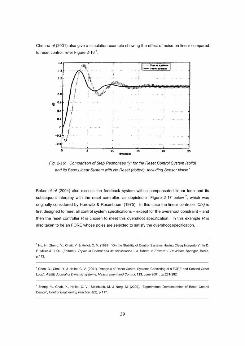
39
Chen et al (2001) also give a simulation example showing the effect of noise on linear compared
to reset control, refer Figure 2-16 4.
Fig. 2-16: Comparison of Step Responses “y” for the Reset Control System (solid)
and its Base Linear System with No Reset (dotted), Including Sensor Noise 4
Beker et al (2004) also discuss the feedback system with a compensated linear loop and its
subsequent interplay with the reset controller, as depicted in Figure 2-17 below 2, which was
originally considered by Horowitz & Rosenbaum (1975). In this case the linear controller C(s) is
first designed to meet all control system specifications – except for the overshoot constraint – and
then the reset controller R is chosen to meet this overshoot specification. In this example R is
also taken to be an FORE whose poles are selected to satisfy the overshoot specification.
_______________________________________________________________________________________________________________________
3 Hu, H., Zheng, Y., Chait, Y. & Hollot, C. V. (1999). “On the Stability of Control Systems Having Clegg Integrators”, In D.
E. Miller & Li Qiu (Editors.), Topics in Control and its Applications – a Tribute to Edward J. Davidson, Springer, Berlin,
p.113. _______________________________________________________________________________________________________________________
4 Chen, Q., Chait, Y. & Hollot, C. V. (2001). “Analysis of Reset Control Systems Consisting of a FORE and Second Order
Loop”, ASME Journal of Dynamic systems, Measurement and Control, 123, June 2001, pp.281-282. _______________________________________________________________________________________________________________________
5 Zheng, Y., Chait, Y., Hollot, C. V., Steinbuch, M. & Norg. M. (2000). “Experimental Demonstration of Reset Control
Design”, Control Engineering Practice, 8(2), p.117. _______________________________________________________________________________________________________________________

40
Fig. 2-17: Reset Control Design Involves Interplay Between Linear Loop P(s).C(s)
and the Reset Controller R 2
Table 2-1 and 2-2 summarize the cases in the literature that used the reset control design
methods described in Figure 2-11 and 2-17 respectively. They also indicate whether the reset
controller R used was a Clegg Integrator or a FORE.
Table 2-1: Summary of Cases in the Literature Using Reset Control Design Method R+P(s)
Ref. Closed-loop System R C(s) P(s) Reset to
Zero Clegg
(1958) R+P(s) Clegg Yes
Hu, Zheng, Chait & Hollot
(Jun 1997) R+P(s) Clegg
LTI plant,
where P(s)= 1st order, 2nd order,
3rd order, and higher order
Yes
Hollot, Zheng & Chait
(Dec 1997) R+P(s) Clegg Yes
Hu, Zheng, Chait & Hollot
(1999) R+P(s) Clegg
LTI plant,
where P(s)= 1st order, 2nd order,
3rd order, and higher order
Yes
Beker, Hollot & Chait
(Jun 1999) R+P(s) FORE Yes
Beker, Hollot & Chait
(Nov 2001 a) R+P(s) FORE P(s)=1/s Yes
Beker, Hollot, Chait & Han
(2004) R+P(s)
R+C(s)+P(s) FORE Yes
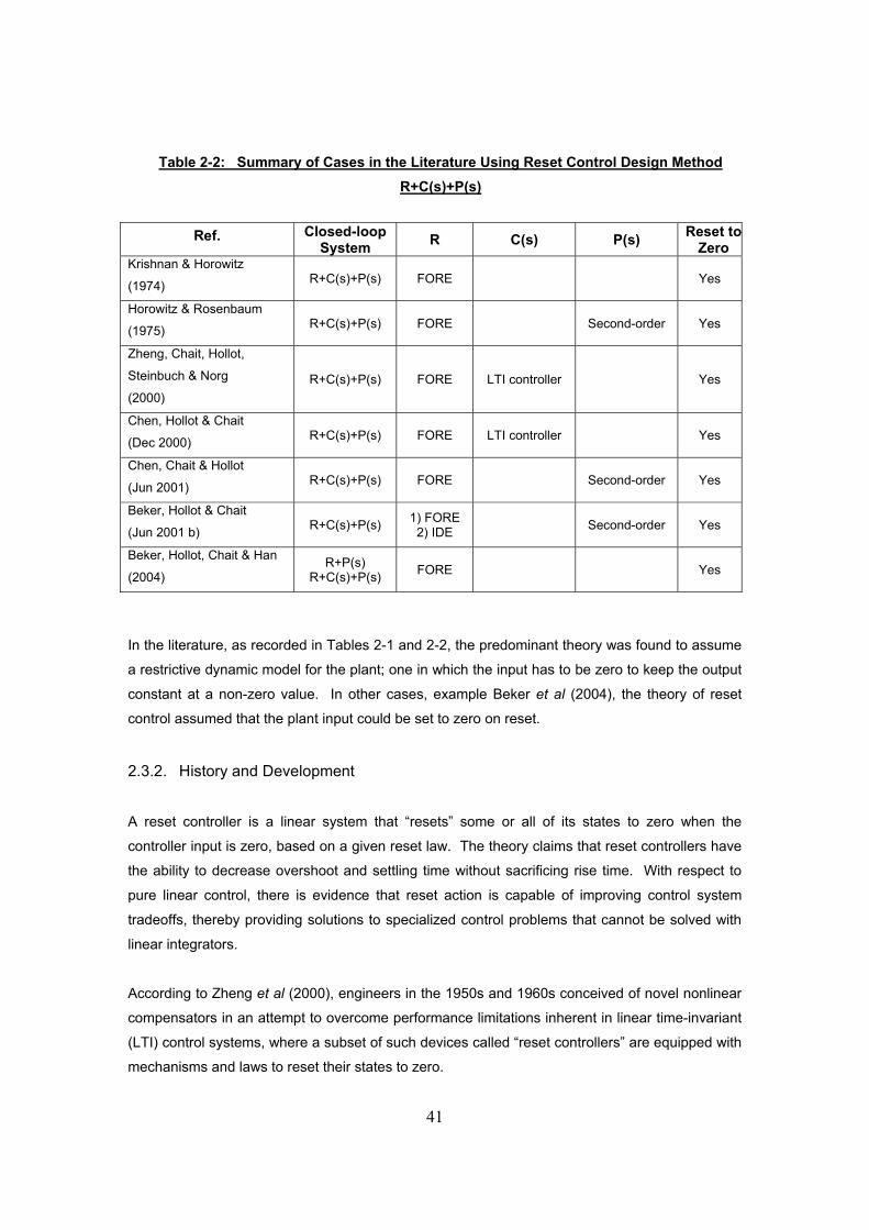
41
Table 2-2: Summary of Cases in the Literature Using Reset Control Design Method R+C(s)+P(s)
Ref. Closed-loop
System R C(s) P(s) Reset toZero
Krishnan & Horowitz
(1974) R+C(s)+P(s) FORE Yes
Horowitz & Rosenbaum
(1975) R+C(s)+P(s) FORE Second-order Yes
Zheng, Chait, Hollot,
Steinbuch & Norg
(2000) R+C(s)+P(s) FORE LTI controller Yes
Chen, Hollot & Chait
(Dec 2000) R+C(s)+P(s) FORE LTI controller Yes
Chen, Chait & Hollot
(Jun 2001) R+C(s)+P(s) FORE Second-order Yes
Beker, Hollot & Chait
(Jun 2001 b) R+C(s)+P(s) 1) FORE 2) IDE Second-order Yes
Beker, Hollot, Chait & Han
(2004) R+P(s)
R+C(s)+P(s) FORE Yes
In the literature, as recorded in Tables 2-1 and 2-2, the predominant theory was found to assume
a restrictive dynamic model for the plant; one in which the input has to be zero to keep the output
constant at a non-zero value. In other cases, example Beker et al (2004), the theory of reset
control assumed that the plant input could be set to zero on reset.
2.3.2. History and Development
A reset controller is a linear system that “resets” some or all of its states to zero when the
controller input is zero, based on a given reset law. The theory claims that reset controllers have
the ability to decrease overshoot and settling time without sacrificing rise time. With respect to
pure linear control, there is evidence that reset action is capable of improving control system
tradeoffs, thereby providing solutions to specialized control problems that cannot be solved with
linear integrators.
According to Zheng et al (2000), engineers in the 1950s and 1960s conceived of novel nonlinear
compensators in an attempt to overcome performance limitations inherent in linear time-invariant
(LTI) control systems, where a subset of such devices called “reset controllers” are equipped with
mechanisms and laws to reset their states to zero.

42
Subsequent to Clegg’s initial work in 1958 (Clegg, 1958), the study of reset control does not
resurface until some 20 years later in the mid 1970’s – Krishnan & Horowitz (1974) and Horowitz
& Rosenbaum (1975). But despite its demonstrated potential, reset control remained relatively
obscure on the modern control scene. Zheng et al (2000) suggests that this is because either
real-time implementation of reset control laws may have challenged the technologies of the 1950s
to 1970s, or there was a lack of sharp theoretical results to firmly establish the stability and
performance properties of these reset control systems.
Some 20 years after the work of Horowitz & Rosenbaum (1975), during the late 1990’s, there
seemed to be a revival of interest in reset control, both from a theoretical and applications point of
view. However, one missing element of this work was a concrete example showing that reset
control meets the control system objectives that are unattainable over all linear controllers.
The renewed interest in the topic was spurred by Zheng et al (2000) and Chen et al (2000) who
both demonstrated experimentally the concepts developed by Horowitz & Rosenbaum (1975), for
the first time.
The potential advantages of using Clegg integrators and reset control had now been
demonstrated in the literature via both simulations and experiments. This experimental evidence
supplied a basis for further analytical and theoretical study, which was then followed by a series
of papers exploring the stability of reset control, which was missing from the previous research.
The main developments and contributions of the various authors to reset control over the years
are summarized chronologically in the Table 2-3 below, which also indicates whether the results
were obtained via theoretical simulation or actual experiments.

43
Table 2-3: Chronological Account of Contributions to Reset Control in the Literature
Clegg (1958). “A Nonlinear
Integrator for Servomechanisms”.
Initiated work on reset elements through desire to overcome inherent limitations of linear feedback control, in an attempt to improve the trade-offs amongst competing control objectives. Applied the reset concept to an integrator element. Paper describes a non-linear integrator (the Clegg Integrator), which is superior in respect to the linear type. Hence the Clegg Integrator – which is a linear integrator whose output resets to zero whenever its input crosses zero, or that zeros the integrator state (1/s) – is a classic example of reset controller. Seems possible that the Clegg Integrator can provide solutions to specialized control problems that cannot be solved with linear integrators. Analysis limited to describing functions.
Krishnan & Horowitz (1974). “Synthesis of a Non-linear
Feedback System with Significant
Plant-ignorance for Prescribed
System Tolerances”.
Established a design technique to exploit the apparent advantages of the Clegg Integrator (Clegg, 1958) in robust control. However, its successful usage hinges on the ability to analyze its closed-loop stability, and such behaviour was not yet fully established. Made an attempt to systematically and quantitatively incorporate a Clegg Integrator into a control system design. In so doing, Clegg Integrator concept was extended to first order reset elements (FOREs), without recourse to describing functions. Focused on the compensated linear loop and its subsequent interplay with the reset controller as shown in Figure 2-17 for R+C(s)+P(s), where R=FORE. Advocated a two-step process where first designed the linear controller C(s) to meet all control system specifications, except for the overshoot constraint, then selected the FORE’s pole to meet this overshoot specification. Demonstrated by simulations, but ignored stability issues altogether. Work was supported by computer simulations at the time, which showed that reset control could provide better trade-offs than linear time-invariant (LTI) control. Also showed that improved performance did not come from a “blind resetting” of an LTI controller, but from a distinct and intentional interplay between the reset mechanism and an appropriately designed LTI controller component.
Horowitz & Rosenbaum (1975). “Non-linear Design for Cost of
Feedback Reduction in Systems
with Large Parameter
Uncertainty”.
Through design methodologies and simulations, supported the possibility that Clegg Integrator (Clegg, 1958) can provide solutions to specialized control problems that cannot be solved with linear integrators. Clegg Integrator concept used by Krishnan & Horowitz (1974) was advanced by extending to first-order lag filter, so-called first order reset elements (FOREs), and quantitatively incorporated them into control system design, without recourse to describing functions. Focused on the compensated linear loop and its subsequent interplay with the reset controller as shown in Figure 2-17 for R+C(s)+P(s), where R=FORE.

44
Advocated a two-step process where first designed the linear controller C(s) to meet all control system specifications, except for the overshoot constraint, then selected the FORE’s pole to meet this overshoot specification. Generalized the resetting concept to higher-order systems. Provide specific guidelines for this choice which explicitly link the design of reset controllers to the linear compensation, and showed that resetting action reduces overshoot. However, considerations of closed-loop stability not addressed. Lacked any stability analysis. Zheng et al (2000) state that the key element in reset control is the design of a base, linear control system with small gain/phase margins. The effect of introducing reset is to increase these margins without sacrificing the benefits derived from such linear controllers. This is achieved by designing the reset action to improve transient performance. It is in this context that Horowitz & Rosenbaum (1975) made a connection between reset action, the linear control element and reduced overshoot. In 2000, their design rule constituted the only concrete guideline for designing reset controllers, however, the scope of this guideline was limited. Specifically, their design rule guarantees only that if the linear closed-loop step system is second-order, then the first peak in the step response of the reset control system is reduced to a certain amount. Demonstrated by simulations, but ignored stability issues altogether. Work was supported by computer simulations at the time, which showed that reset control could provide better trade-offs than linear time-invariant (LTI) control. Also showed that improved performance did not come from a “blind resetting” of an LTI controller, but from a distinct and intentional interplay between the reset mechanism and an appropriately designed LTI controller component.
Tsypkin (1984). “Relay Control
Systems”.
Noted by Chen et al (2000) and Beker et al (2004): Reset control resembles a number of popular nonlinear control strategies, including relay control described by Tsypkin (1984). A common feature is the use of a switching surface to trigger change in control signal. Distinctively, reset control employs the same (linear) control law on both sides of the switching surface (defined by e = 0). Resetting occurs when the system trajectory impacts this surface. This reset action can be alternatively viewed as the injection of judiciously timed, state dependent impulses into an otherwise linear time-invariant (LTI) feedback system.
DeCarlo, Zak & Matthews (1988). “Variable Structure Control of
Nonlinear Multivariable Systems:
A Tutorial”.
Noted by Chen et al (2000) and Beker et al (2004): Reset control resembles a number of popular nonlinear control strategies, including sliding mode control described by Decarlo et al (1988). Common feature is a switching surface used to trigger change in control signal. Distinctively, reset control employs the same (linear) control law on both sides of the switching surface (defined by e = 0). Resetting occurs when the system trajectory impacts this surface with reset action producing a jump in the system trajectory. This reset action can be alternatively viewed as the injection of judiciously timed, state-dependent impulses into an otherwise linear time-invariant (LTI) feedback system.

45
Singer & Seering (1990).
“Preshaping Command Inputs to
Reduce System Vibration”.
Noted by Chen et al (2000) and Beker et al (2004): The connection of reset control to impulsive control helps draw comparison to body of control work where impulses are introduced in an open-loop fashion to quash oscillations in vibratory systems.
Bobrow, Jabbari & Thai (1995).
“An Active Truss Element and
Control Law for Vibration
Suppression”.
Noted by Beker et al (2001a, 2004): Other research on reset-like control where resetting actuators were used to suppress mechanical vibrations. Demonstrates that reset control having different set of performance limitations can be exploited in specific control applications.
Yamamguchi (1997). “A Mode-
switching Controller with Initial
Value Compensation for Hard Disk
Drive Servo Control”.
Noted by Zheng, Y. et al (2000): Authors show that mode-switching control, which consists of several controllers and a scheme for switching from one controller to another, can improve the performance of a hard servo disk by making favourable trade-offs between fast movement and precise positioning. This type of control is a non-linear scheme which is related to reset control. However, while mode-switching control utilizes a number of linear loop designs, reset control involves a potentially simpler, single-loop design and uses reset action to alter the linear loop to achieve improved closed-loop behaviour.
Feuer, Goodwin & Salgado (Jun 1997). “Potential Benefits of
Hybrid Control for Linear Time
Invariant Plants”.
Noted by Beker et al (2004): Other research on reset-like control where potential benefit of using switched compensators for controlling linear plants was explored. Switching control, a nonlinear scheme analogous to reset control, exhibits similar advantages over linear controllers.
Hu, Zheng, Chait & Hollot (Jun 1997). “On the Zero-Input Stability
of Control Systems with Clegg
Integrators”.
According to Zheng et al (2000), although the ability of reset control to perform better than linear control appears optimistic, a number of theoretical questions need to be formulated and answered before reset control can be embraced as a viable control engineering tool and Hu et al (1997) begin to address some of these issues. Considered negative-feedback system consisting of a single-input, single output, linear time-invariant (LTI) plant with R+P(s) as shown in Figure 2-11, where R=Clegg Integrator and P(s)= first order, second order, third order, and higher order transfer functions. Necessary and sufficient conditions for internal stability are given for a restricted class of systems characterized by a Clegg Integrator and second-order plant, as well as preliminary results for higher order plants. Paper completely resolves the question of zero-input stability for a negative feedback system involving a Clegg Integrator and second-order plant transfer function. First, show that Clegg Integrator resets periodically, then prove that stability can be deduced from an underlying linear shift-invariant discrete-time system.

46
The closed-loop system with Clegg Integrator resets at most once and behaves linearly thereafter. The Clegg Integrator resets periodically (zero-crossings of y(t) are evenly spaced) when in feedback with a second-order plant. This reduces the stability problem to a linear, shift-invariant discrete-time problem. Illustrate this stability condition with a simple example, where y(t) either has an infinite number of periodically-spaced zero-crossings or at most, one crossing. In the latter case, the closed-loop system is zero-input stable only if P(s) is stabilized by a linear integrator. In the former case, stability may be deduced from the state ‘s behaviour at these periodic instances. Their main result exploits this periodicity and gives a stability condition in terms of a shift-invariant, discrete-time system. Example shows that a plant stabilized by a linear integrator may or may not be stabilized by a Clegg Integrator, however, a plant may be stabilized by the Clegg Integrator even though it is not stabilized by the linear integrator. Also provide an example to show how reset can destabilize a stable linear feedback system, even when the describing function suggests otherwise. When connected to higher-order plants exhibit more complex reset patterns. Give some preliminary results for higher-order plants and state a sufficient condition for stability. For an n-th order plant, the largest number of zero crossings is n-1 and the Clegg Integrator eventually behaves as a linear integrator which is assumed to stabilize the plant. Paper shows the need for more comprehensive stability condition but does not provide the necessary theoretical machinery, since analysis based on exact characterization of reset times which appears to be an impossible task for higher-order plants.
Hollot, Zheng & Chait (Dec 1997).
“Stability Analysis for Control
Systems with Reset Integrators”.
According to Zheng et al (2000), although the ability of reset control to perform better than linear control appears optimistic, a number of theoretical questions need to be formulated and answered before reset control can be embraced as a viable control engineering tool and Hollot et al (1997) begin to address some of these issues. Considered example of reset integrator control system involving feedback loop incorporating Clegg integrator and transfer function, i.e. R+P(s) as shown in Figure 2-11, where R=Clegg Integrator. Introduced integral quadratic constraint (IQC) models to represent the nonlinear action of state reset action, and developed some stability criteria for such systems. However, these particular representations gave more conservative stability conditions. Study the stability of closed-loop systems incorporating reset integrators. Generally, the stability analysis for such systems involves two steps: 1) Determination of possible reset patterns; 2) Stability analysis for each possible reset pattern. Since reset action is determined from a set of pre-fixed, state-dependant rules, reset patterns can be complex and dependent on the control system’s signals & initial conditions. The stability analysis taken in this paper assumes only bounds on the reset times, and consequently the study guarantees stability for any reset pattern satisfying these bounds. Based on this assumption of uncertain-but-bounded reset intervals, they model integrator reset action as an impulse modulator with uncertain impulse times.

47
Branicky (1998). “Multiple
Lyupanov Functions and Other
Analysis Tools for Switched and
Hybrid Systems”.
Noted by Chen et al (2000) and Beker et al (2004): Reset control resembles a number of popular nonlinear control strategies, including switching control described by Branicky (1998). A common feature is the use of a switching surface to trigger change in control signal. Distinctively, reset control employs the same (linear) control law on both sides of the switching surface (defined by e = 0). Resetting occurs when the system trajectory impacts this surface. This reset action can be alternatively viewed as the injection of judiciously-timed, state dependent impulses into an otherwise LTI feedback system.
Ye, Michel & Hou (Dec 1998). “Stability Analysis of Systems with
Impulse Effects”.
Study of impulsive differential equations (IDEs). Analysis required assumptions of reset times. Help establish a general Lyapunov theory for reset control system, which is a special case of impulsive differential equations and hybrid dynamical systems. Established conditions for the uniform stability and the uniform asymptotic stability of equilibria of systems with impulse effects described by systems of non-linear, time-varying, ordinary differential equations. Under mild additional assumptions, these sufficient conditions turn out to be necessary as well. For the case of time-invariant systems with impulse effects described by non-linear ordinary differential equations, the above results are used to establish conditions under which the uniform asymptotic stability of equilibria can be deduced from linearizations of such systems. Work presented in three parts: First, present the description of the class of systems with impulse effects considered and summarize existing stability results; Second, present new stability results for this system; Third, present converse stability results for this system.
Haddad, Chellaboina & Kablar
(1999). “Nonlinear Impulsive
Dynamical Systems Part I:
Stability and Dissipativity”.
Noted by Chen et al (2000): This reset action can be alternatively viewed as the injection of judiciously-timed, state dependent impulses into an otherwise LTI feedback system. This analogy is evident where they use impulsive differential equations (IDEs) to model dynamics.
Hu, Zheng, Chait & Hollot (1999).
“On the Stability of Control
Systems Having Clegg
Integrators”.
Study internal stability of feedback systems with Clegg Integrator, and provide stability conditions when the plant is second order as well as preliminary results for higher order classes. Provide techniques which can be used to deduce stability. Considered negative-feedback system consisting of a single-input , single output, linear time-invariant (LTI) plant as shown in Figure 2-11, with R+P(s) where R=Clegg Integrator and P(s) = first order, second order, third order, and higher order transfer functions. First analyze the behaviour of a Clegg Integrator in feedback with a first order plant. Begin a study of stability analysis for feedback systems using Clegg Integrator, and report some first results which help characterize the internal stability of a feedback interconnection of a Clegg Integrator with a second-order plant.

48
Show that if the Clegg Integrator continually resets, then it must reset periodically, and the periodic rate can be determined a priori from the plant description. As a consequence, internal stability can be deduced from an implicit shift-invariant discrete-time system. The closed-loop system with Clegg Integrator resets at most once and behaves linearly thereafter. The Clegg Integrator resets periodically when in feedback with a second-order plant. When connected to higher-order plants exhibit more complex reset behaviour, but at this stage of the research, they have not characterized these patterns. However, for an n-th order plant, they can predict that the Clegg Integrator will reset n-1 times at most. Give conditions for which the Clegg Integrator resets only a finite number of times. In these cases, the internal stability of the closed-loop system depends solely on whether the plant is stabilized by a linear integrator. For these higher-order systems, future research will focus on input-output stability, and reset behaviour is input dependent. Demonstrate that some reset control systems are not quadratically stable by showing that a Clegg integrator exponentially stabilizes the plant P(s) while this plant cannot be stabilized by a linear integrator. In this case application of reset destabilizes a stable base-linear system and hence is of no benefit over the linear system. Results show that a plant stabilized by a linear integrator can either remain stabilized or be destabilized by a Clegg Integrator. Conversely, a plant which is destabilized by a linear integrator can exhibit stable initial condition response even though this same initial condition excites unstable modes in the related linear feedback system.
Beker, Hollot & Chait (Jun 1999).
“Stability of a Reset Control
System Under Constant Inputs”.
Consider reset system R+P(s) as shown in Figure 2-11, where R=FORE. In the absence of resetting, the FORE behaves like a linear system 1/(s+b). Showed that equilibrium point for the reset control system is asymptotically stable if r, d or n is a constant signal (refer Figure 2-11). For constant reference signal r and any initial condition, the tracking error e asymptotically converges to zero. A breakthrough was reported, which gave a testable Lyapunov-based stability condition (referred to as the Hβ-condition) achieved by avoiding direct use of reset times and delineating dynamic behaviour along the set of reset states. Analysis required assumptions of reset times.
Haddad, Chellaboina & Kablar
(Jun 2000). “Active Control of
Combustion Instabilities via Hybrid
Resetting Controllers”.
Noted by Beker et al (2001a, 2004): Other research on reset-like control where so-called hybrid resetting controllers were used to control combustion instabilities. Demonstrates that reset control having different set of performance limitations can be exploited in specific control applications.
Bupp, Bernstein, Chellaboina &
Haddad (2000). “Resetting Virtual
Absorbers for Vibration Control”.
Noted by Beker et al (2001a, 2004): Other research on reset-like control where resetting actuators were used to suppress mechanical vibrations. Demonstrates that reset control having different set of performance limitations can be exploited in specific control applications.

49
Lau & Middleton (Dec 2000). “On
the Use of Switching Control for
Systems with Bounded
Disturbances”.
Noted by Beker et al (2004): Other research on reset-like control where the potential benefit of using switched compensators for controlling linear plants was explored.
Zheng, Chait, Hollot, Steinbuch &
Norg (2000). “Experimental
Demonstration of Reset Control
Design”.
Note that reset control is only one among a number of nonlinear schemes intended to improve on linear control, and mention a number of related techniques which resemble reset control (see Yamamguchi example above). Noted by Beker et al (2001a): Demonstrate that reset control having different set of performance limitations can be exploited in specific control applications. Through design methodologies, simulations and experiments, they supported the possibility that the Clegg integrator can provide solutions to specialized control problems that cannot be solved with linear integrators. Paper reports on a design procedure and laboratory experiment for speed control of a tape-drive system to demonstrate the concepts developed by Horowitz & Rosenbaum (1975), in which the resulting reset controller provides better design trade-offs than LTI compensation. This system represents a control problem that is difficult, if not impossible, to satisfy the performance using a LTI controller. Authors claim that this is the first physical experiment of this type to be reported in the literature. Like Horowitz & Rosenbaum (1975) their design and development of the reset control system involves the two-step synthesis of both linear compensator C(s) and reset controller R where, typically, the C(s) is used to stabilize and shape the loop to satisfy classical Bode specifications at high and low frequencies and the reset controller is then designed to meet overshoot constraints. Therefore, they Consider R+C(s)+P(s) as shown in Figure 2-17, where R=FORE, C(s)=LTI controller. In their experiment they design the C(s) loop (referred to as GL in the paper) to satisfy both sensor-noise suppression and disturbance-rejection specifications, after which they design the reset controller R (referred to as GR in the paper) as a FORE, similar to Horowitz & Rosenbaum (1975). This reset controller consists of a first-order linear filter with logic to reset the filter state to zero when its input e crosses zero and is described by a reset differential equation similar to equation [2.14] above:
xI = –bx + e, e ≠ 0, x = 0, e = 0, u = x
where x is the state and where the filter’s pole b > 0, and essentially GR is a reset version of the linear element 1/(s+b). It is specifically shown that reset control applied to this system increases the level of sensor-noise suppression (by almost double) without sacrificing either disturbance-rejection performance or gain/phase margins, and caters for disturbance rejection. The reset control meets the performance specifications that linear control was unable to satisfy.

50
Simulations show that improved performance does not come from “blind” resetting of an existing LTI controller, instead, it comes from distinct and intentional interplay between the reset mechanism and an appropriately designed LTI controller. They state that the key element in reset control is the design of a base, linear control system with small gain/phase margins. The effect of introducing reset is to increase these margins without sacrificing the benefits derived from such linear controllers. This is achieved by designing the reset action to improve transient performance. Demonstrate by simulations and experiment, however, application of small gain appears too conservative and could not validate the observed experimental performance. It is in this context that Horowitz & Rosenbaum (1975) made a connection between reset action, the linear control element and reduced overshoot. In 2000, their design rule constitutes the only concrete guideline for designing reset controllers, however, the scope of this guideline is limited. Specifically, their design rule guarantees only that if the linear closed-loop step system is second-order, then the first peak in the step response of the reset control system is reduced to a certain amount. They demonstrate through both simulations and real-time experiments that reset control has the ability to perform better than linear control but do not guarantee factors such as stable response to step disturbances (response of reset control system may not converge); behaviour when sinusoidal and sensor noise is introduced; disturbance rejection and sensor-noise suppression performance (reset control system may not inherit the good performance properties of linear design); overshoot reduction in terms of global maximum versus first peak. They discuss the shortcomings of reset control and conclude that although the ability of reset control to perform better than linear control appears optimistic, a number of theoretical questions need to be formulated and answered before reset control can be embraced as a viable control engineering tool.
Chen, Hollot & Chait (Dec 2000).
“Stability and Asymptotic
Performance Analysis of Reset
Control Systems”.
Objective was to provide level of analysis previously missing in past work on reset control. Demonstrated the concepts of Horowitz & Rosenbaum (1975) by setting up a model to describe the reset control system, identifying key underlying linear control system (referred to as base-linear control system), then applying the stability results experimentally on a rotational flexible mechanical system (tape-speed servo control). Use R+L(s) where R=FORE and L(s) denotes the linear loop consisting of the plant and any linear compensation, i.e. C(s)+P(s), as shown in Figure 2-17. Assumed the FORE continually resets to avoid degeneration to an LTI system. Spurred by the confirmation of internal stability of the experimental demonstration by Zheng et al (2000), Chen et al (2000) continued the work establishing BIBO (bounded-input, bounded output) stability, asymptotic tracking and stability, and steady-state performance for reset control systems employing FOREs. Their analysis required assumptions of reset times.

51
A bounded-input bounded-output (BIBO) stability result was given for a special class of reset control systems that utilize FOREs, and assumed that the reset intervals were lower bounded. Introduced the β positive-real condition, which, when satisfied allows one to assert BIBO and asymptotic stability of the reset control system. Used the Hβ-condition to establish stability of experimental demonstrations in reset control, thus confirming the observed stability and demonstrating the applicability of their results. Under this condition, also show that the reset control system inherits the steady-state tracking properties of an underlying linear control system. Show it is possible that a reset control system is unstable even though its base-linear system is stable and describing-function analysis does not predict a limit-cycle. Introduce robustness to implementation errors. Reset control implicitly assumes that the reset process is ideal, that is, the FORE resets to exactly zero at the precise instant when its input e(t) is zero. Realistically, this seldom happens as exemplified by the digital implementation of reset elements where such errors occur due to finite sampling rates and signal quantization. To account for such inaccuracies, they modify the reset control accordingly to bounded signals. Note that the BIBO stability condition remains valid despite these implementation errors. This reset action can be alternatively viewed as the injection of judiciously-timed, state dependent impulses into an otherwise LTI feedback system. This analogy is evident where they use impulsive differential equations (IDEs) to model dynamics. Despite this relationship, they found the existing theory on IDEs to be either too general or too broad to be of immediate and direct use.
Beker, Hollot & Chait (Dec 2000).
“Forced Oscillations in Reset
Control Systems”.
Have laid some groundwork for determining the performance of reset control systems to sensor noise by evaluating the system gain from sensor noise to plant output, where they have studied the steady-state response of reset control systems to sinusoidal sensor noise and in some simple examples have computed the steady-state gain. These gains agree well with results obtained using a sinusoidal describing function approximation of the reset controller. In analyzing the response of a class of reset control systems to oscillations forced by sinusoidal sensor noise, they show that limit cycles exist, give a condition under which the limit cycles can be considered as simple, and suggest that immediate future research directions should include the stability analysis of limit cycles.
Chen, Chait & Hollot (Jun 2001).
“Analysis of Reset Control
Systems Consisting of a FORE
and Second Order Loop”.
Introduce the dynamics of reset control systems. Also conducted transient-response analysis for second-order plants. Consider closed-loop system as shown in Figure 2-17, R+C(s)+P(s) where reset controllers consist of two parts – linear compensator and reset element. The linear compensator C(s) is first designed in the usual ways to meet all closed-loop performance specifications while relaxing the overshoot constraint, then the reset element R is chosen to meet this remaining transient step-response specification. The reset element is simply a filter whose output is reset to zero when the filter input is zero – special cases include the Clegg integrator and first-order reset element (FORE).

52
Focus on the special case where such linear compensation results in second-order (loop) transfer function and where a first order reset element (FORE) is employed, i.e. where R=FORE. Analyse the closed-loop reset control system addressing performance issues such as stability, steady-state response, and transient performance. Concentrate on situation where the linear design results in loop transfer function L(s) = P(s).C(s) dominated by a complex pole pair. Give a testable (as opposed to general) condition for asymptotic and quadratic stability that is both necessary and sufficient. Give a stronger BIBO stability condition. Simpler setup considered allows them to fully characterize the step response, and also allow them to draw comparison to classical linear control systems described by second-order transfer functions. Give sharp results for asymptotic and BIBO stability, asymptotic tracking of constant inputs and transient-response properties such as rise time, overshoot, settling time. Provide stability and steady-state performance results for reset control systems consisting of more general reset elements and linear loops P(s).C(s). Have yet to characterize response of these reset control systems to high-frequency sensor noise, to give a better picture of trade-offs faced by reset control systems.
Beker, Hollot & Chait (Jun 2001 b). “Stability of Limit Cycles in
Reset Control Systems”.
State that the existence of solutions in reset control systems is closely related to ruling out “fast switches” in relay control systems, but for the reset control systems the possibility of such a phenomenon is still under investigation. Continue work on establishing properties of reset control systems. Consider reset system R+C(s)+P(s), as shown in Figure 2-17, where R=IDE (Impulsive Differential Equation) in one example, and an R=FORE applied to a second-order plant in a second example. Focus on local stability of limit-cycles induced under sinusoidal sensor excitation. Give an example of a reset control system (second order plant utilizing a FORE), show that the limit-cycle it generates is simple and establish the local stability thereof. Some groundwork for determining the performance of reset control systems to sensor noise by evaluating the system gain from sensor noise to plant output has been laid here where they have studied the steady-state response of reset control systems to sinusoidal sensor noise and in some simple examples have computed the steady-state gain. These gains agree well with results obtained using a sinusoidal describing function approximation of the reset controller.
Beker, Hollot & Chait (Nov 2001 a). “Plant with Integrator: An
Example of Reset Control
Overcoming Limitations of Linear
Feedback”.
Introduced a concrete example which demonstrates theoretically that reset control can meet specifications requiring balance between tracking and rise time performance without overshooting, whereas any linear feedback system would overshoot when meeting the same requirements. Consider R+P(s), as shown in Figure 2-11, where R=FORE and P(s)=1/s (simple integrator). Reset to zero.

53
Introduce an overshoot limitation on linear feedback systems arising when the loop contains an integrator. This result is an immediate consequence of the time-domain limitations, but give an example showing reset control does not suffer this limitation. Two-fold purpose: First, to give conditions under which linear feedback control of a plant containing integrator must overshoot. Second: to give example of reset control that does not overshoot under such constraints. Paper concludes that this example does not imply that reset control is superior, but rather that reset control has a different set of performance limitations, which could be exploited in specific control applications. According to the authors, this is the first definitive example showing the benefit of reset control over linear feedback and is a significant milestone in the development of reset control. Clearly shows the benefit of reset control.
Beker, Hollot, Chait & Han (2004). “Fundamental Properties of Reset
Control Systems”.
Note a number of related techniques which resemble reset control (see above). Use impulsive differential equations (IDEs) to model the dynamics of reset control in order to establish some fundamental closed-loop properties for application of reset control in their feedback connection to linear plants. Set up the reset control problem by expressing the dynamics of reset in terms of impulsive differential equations. Consider closed-loop R+P(s), as shown in Figure 2-11, where R=FORE. Also consider more general reset structures than previous work, which allows for higher order controllers and partial-state resetting. First establish the conditions for input-output systems, then draw their attention to the steady-state performance of reset control systems and establish an internal model principle similar to that found in linear control systems. The properties investigated for these closed-loop reset systems include stability, asymptotic tracking, disturbance rejection and steady-state performance. State Lyapunov-based stability conditions for closed-loop stability, give necessary and sufficient condition for quadratic stability. Show the Lyapunov-based stability condition (referred to as the Hβ-condition) is necessary and sufficient for quadratic stability and links it to both uniform bounded-input bounded-state (UBIBS) stability and asymptotic tracking. Establish that the Hβ-condition is a strict positive real constraint on the base-linear system and amounts to a requirement over and above the base-linear stability, and which is useful in establishing other properties of reset control systems. Also distinguish that there is a difference in the classes of reset systems that are stable and quadratically stable, and that there exists a rich class of reset control systems that are quadratically stable. For linear systems, quadratic stability is tested via a Lyapunov equation. For reset control systems, it is deduced from a constrained Lyapunov equation, or equivalently, from a strict positive real (SPR) condition (the Hβ-condition). All stable linear systems are quadratically stable, but not so for reset control. Nevertheless, the Hβ-condition has been valuable in establishing stability for some higher-order experimental systems.

54
Paper shows that quadratic stability plays an important role in reset control systems, similar to that in linear feedback, meaning that quadratically stable reset control systems are input-output stable and have an internal model property useful in asymptotic tracking and disturbance rejection. Suggest that incorporating the Hβ-condition into controller synthesis would appear to be a worthwhile objective allowing one to bring quadratic stability directly into the design process. Unlike any previous work, which includes the study of impulsive differential equations, their paper also contributes stability results that require no assumptions on the evolution of reset times. Understanding that in general reset elements do not enjoy superposition, they question how tracking error is affected by sensor noise. Their work complements previous related research which shows the potential benefit of reset control either through theory, simulation or experiment. Experimental demonstrations of reset control in Zheng et al (2000) and Chen et al (2000) verified to be quadratically stable, and associated loop transfer functions were non-trivial. Suggest that a possible topic for further research is to explore the use of non-quadratic Lyapunov functions. Another topic for future research is concerned with the performance of reset control systems to sensor noise, where they would like to evaluate the system gain from sensor noise to plant output. Finally, some other areas of future research include robustness, controller synthesis and performance limitations. Robustness of results with regards to hi-frequency parasitics is an open issue and generalizing this to a more general norm-bounded uncertain dynamic would also be of interest. Lastly, boundaries defining the potential benefits and cost for using reset control have yet to be drawn. A formal study of the performance limitations of reset control systems appears ripe and challenging.

55
3. CONTROL STUDY AND OPTIMIZATION OF EXISTING SYSTEM 3.1. Control Study Method
From the literature search it was noted that reset controllers are generally implemented on
optimal control solutions so the existing operation and control needed to be thoroughly
investigated and optimized first. The in-depth control study – which forms the main focus of the
thesis – identified an array of practical issues that could readily be rectified. Some of these
existing control problems had to be addressed first in order to quantify the benefits that would
result from implementation of a reset controller in this industrial process.
Owing to the varied nature and complex chemistry of the industrial PGM dissolve process, the
original aim of the industrial reactor project was to develop a fundamental understanding of the
process hydrometallurgy, equipment design and control through research and in-depth analysis
of the current operation, with a view to improve its existing control, operability and performance
efficiency. It is important for control to select sensible process and manipulated variables, and
this requires a detailed understanding of the process.
For this purpose, a general Control System Design Strategy was formulated – Lahee (2004,
2005a, 2005b, 2006b) – based on a fundamental understanding of each process and its control,
as laid out in the Control System Design Strategy Flowchart, Lahee (2006a), shown in Figure 3-1.
The strategy incorporates various techniques (example Tree Diagrams) being explored and
developed in-house at the same time by the Anglo Platinum Process Control Department.
The left hand side of the flowchart depicts the methodology followed during the initial phases of
the control study, which involves answering a series of very important process-related questions
that effectively describe the control fundamentals specific to the process. This information is
necessary in order to gain a fundamental understanding of the process thereby providing the
information required to define the process in terms of its control. This then forms the foundation
of the final control solution design as depicted on the right hand side of the flowchart.
One should note the magnitude and complexity of the baseline information and hence the tasks
involved to determine it and required before attempting to design the final improved control
solution.

56
It is also important to note from the flowchart that the control system design strategy is an
iterative process that always loops back to having a fundamental understanding of the process,
both during the process definition and final control solution design as well as after its
implementation.
The first step of the Control System Design Strategy – namely gaining a fundamental
understanding of the process – involved an in-depth literature review, including technical and
production reporting, work instructions, control sequences, PLC programming manuals and
interviewing a number of operational personnel from Production, Instrumentation and Process
Control departments. The outcome of the literature review and investigation that describes the
process aspects relevant to the control is contained in Section 2.2.
Through having a fundamental understanding of this specific industrial batch reactor process, the
tree diagram in Figure 3-2, Lahee (2005b), was produced to summarize the reactor process
controllable variables available for manipulation in the existing process.
Figure 3-3 depicts the Functional Tree Diagram, Lahee (2005b), that was populated through
carrying out the Control System Design Strategy. It facilitated the detailed breakdown of the
process and control into distinct functional relationships which in turn enabled interpretation and
deductions to be made in order to understand and describe the multivariable nature of the
process, as summarized in Section 2.2.
A number of graphic visualization techniques developed (by D.V. Groenewald) in MATLAB have
been used to view and analyze the overall control performance before and after optimization.
These include scatter plots, 2D-histogram plots, 2D-density plots, parallel plots and co-variant bi-
plots. Examples of some of these plots are shown in section 3.3 below.
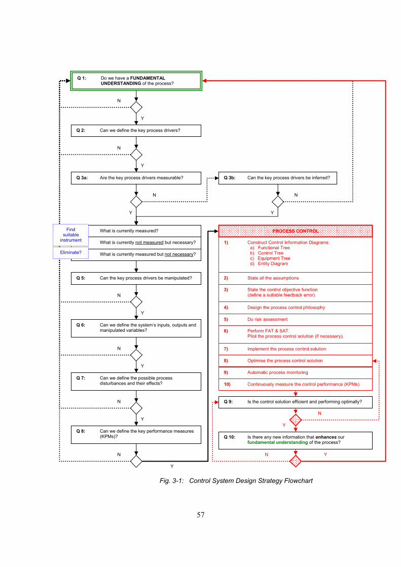
57
Fig. 3-1: Control System Design Strategy Flowchart
1) Construct Control Information Diagrams: a) Functional Tree b) Control Tree c) Equipment Tree d) Entity Diagram
Q 1: Do we have a FUNDAMENTAL UNDERSTANDING of the process?
Q 2: Can we define the key process drivers?
Q 3a: Are the key process drivers measurable? Q 3b: Can the key process drivers be inferred?
Q 5: Can the key process drivers be manipulated?
Q 4c: What is currently measured but not necessary?
Q 4b: What is currently not measured but necessary?
3) State the control objective function (define a suitable feedback error)
4) Design the process control philosophy
7) Implement the process control solution
8) Optimise the process control solution
10) Continuously measure the control performance (KPMs)
9) Automatic process monitoring
Q 8: Can we define the key performance measures (KPMs)?
Q 7: Can we define the possible process disturbances and their effects?
Q 4a: What is currently measured?
Q 9: Is the control solution efficient and performing optimally?
Q 10: Is there any new information that enhances our fundamental understanding of the process?
Y
N
Y
Y
Y
Y
Y
Y
Y
N
N
N
N
N
N
N
Q 6: Can we define the system‘s inputs, outputs and manipulated variables?
N
Y
2) State all the assumptions
5) Do risk assessment
6) Perform FAT & SAT. Pilot the process control solution (if necessary).
PROCESS CONTROL
N Y
Find suitable
instrument
Eliminate?

58
Nomenclature (Figure 3-1):
Key process drivers – Parameters that affect the outcome of the process.
Key performance measures – Parameters that quantify the outcome of the
process.
Functional Tree – Control information tree providing a fundamental description of
the process in terms of its control functionality.
Control Tree – Control information tree describing the regulatory control layers.
Equipment Tree – Control information tree describing the equipment and
instrumentation hierarchy.
Entity Diagram – Information flow diagram showing where to find the data in order to
populate the control information trees with the relevant information.
Fig. 3-2: Reactor Controllable Variables

59
Fig. 3-3: Functional Tree
3.2. Existing Control Solution, Measurements and Manipulated Variables
The existing reactor is controlled through a recipe management system layer on top of a
regulatory control layer consisting mainly of PI controllers. The control sequence executes a
number of process stages wherein it activates or de-activates the PI controllers as required.
The various process steps in the reactor sequence are as follows:
1) Leak test
2) Fill
3) Heat
4) Dissolve
5) Sparge
6) Drain

60
The PI controllers active during the dissolve step are summarized in Table 3-1 below.
Table 3-1: Regulatory Control Layer
No. PI Controller PV MV
1 Temperature control via steam T ST valve
(heating)
2 Temperature control via cooling water T CW valve
(cooling)
3 Chlorine control via flowrate Cl2 Cl2 valve
(Phase I, II and III)
4 Chlorine control via pressure P Cl2 valve
(Phase IV)
5 High Pressure excursion control via vent P Vent valve (entire dissolve)
Fig 3-4 shows how the various PI controllers listed in the table above relate to the batch process
phases described in Section 2.2.3 while Figure 3-5 is a flow diagram representation of how the
sequence loops operate during the dissolve step.
Fig. 3-4: Schematic Representation of Active PI Controllers
P
T

61
Fig. 3-5: Sequence Control Flow Diagram

62
Fig. 3-5: Sequence Control Flow Diagram (continued)

63
3.3. Existing Control Performance Analysis and Optimization 3.3.1. Typical Batch Operation
Figure 3-6 is a typical operating trend demonstrating the control performance achieved under the
existing control philosophy. The sequential batch process phases discussed in Section 2.2.3 and
depicted in Figure 3-4 are also denoted on the trend.
Fig. 3-6: Typical Trend showing Batch Phases
In a typical batch, cooling water is required during phase II, while steam is required during phase
IV. Although the sequence does cater for it, it should not be necessary to frequently switch
between the two during a phase, and this only happens under adverse or trip conditions (example
power or chlorine supply trips).
The in-depth control study has also revealed that the process control performance is heavily
reliant on both mass transfer and cooling capacity, and is readily affected by day-to-day plant
operating problems including an array of equipment and maintenance problems, as well as
interruptions in the chlorine feed supply upstream. Such problems can occur in isolation or in
countless different combinations, and often lead to a multitude of knock-on effects. This results in
a myriad of possible effects which negatively impact the overall control performance.

64
3.3.2. Temperature Control
As shown in Figure 3-7, the temperature of the reactor has been observed to oscillate excessively
with large overshoots and undershoots particularly during Phase II.
The nature of the reactor and jacket design combined with use of a recipe management system
layer (sequence) on top of a regulatory control layer (PI controllers) mimics basic on-off
temperature control. Under this control regime switching between the steam and cooling water
can also occur. The resulting temperature fluctuates on either side of the desired setpoint in a
10oC operating band, as dictated by the control sequence.
Fig. 3-7: Typical Trend showing Temperature Overshoot
Both lag and lead times are present in a temperature control loop of an exothermic reaction such
as in this dissolve process and will always lead to over- and under-shoot of the required limits
with a dominant integral controller, hence oscillation is impossible to avoid. Since the
temperature controller tends to oscillate between the limits the sequence controller is constantly
required to use logic to control the temperature. The control action therefore becomes “crisp”
logic and not a control algorithm that drives the temperature controller. The logic steps between
steam and cooling water control depend on the temperature. The effect of this “crisp” logic
control is further exacerbated by the lag time of the process.

65
The temperature control performance can be manipulated by adjusting the control parameters of
the sequence, such as sequence scan time, jacket drain time, width of temperature dead band
around setpoint and PI tuning parameters. However, the control remains difficult to fine tune.
Figure 3-8 demonstrates a data visualization technique that was developed using MATLAB (by D.
V. Groenewald) to monitor valve performance and detect valve or flowmeter malfunctions or
maintenance requirements. The valve position is plotted against flowrate for each batch. The
data for a number of sequential batches are overlaid, with each batch being given a colour
following the spectrum (earlier batches in red, fading gradually to later batches in blue). If the
valve and flowmeter are well-tuned, well-calibrated and in good operating condition, then the plots
should consistently follow a similar trend, with little or no scatter. Valve position and flowrate
should theoretically have a direct linear relationship.
Figure 3-8 depicts the cooling water control valve performance, where the two plots demonstrate
the difference between the cooling water control valve outputs of two separate but identical
dissolve batch reactors operating in parallel over a one-month period. Although the valve on the
right is controlling accurately, the control profiles have a greater spread and could be addressed,
for example, by using cascade control. Such disturbances in the cooling water supply control can
have a direct effect on the performance of the temperature control loop.
Fig. 3-8: Cooling Water Control Valve Performance – Identical Parallel Reactors

66
3.3.3. Chlorine Flow Control
Because of the multivariable nature of the process (as described in Section 2.2.3), the control of
the chlorine supply, flowrate and dissolution can have a profound impact on the process
temperature response and hence the performance of the temperature control loop.
At times the chlorine main supply is subject to plant trips during the changing of the chlorine
cylinders in the Tankfarm. If it is off for a substantial amount of time, this can disrupt the normal
sequence of events in the batch process since the reactor cools below Tdesign, and then the
sequence has to compensate by re-opening the steam valve in order to reheat the reactor.
Depending on what phase the batch is in at the time, such operation can result in repeated
switching between heating and cooling cycles.
The chlorine plug-flow valve and flowmeter are particularly sensitive and require frequent
calibration and cleaning. The equipment is adversely affected by fluctuations in the upstream
chlorine header pressure and the formation of chlorine butter (especially at low ambient
temperatures). It is also difficult to obtain accurate flow readings at low flowrates with the existing
control valve equipment and instrumentation and the plug-flow valve often leaks through when it
is in the closed position.
Chlorine flow control can have a significant impact on reactor pressure as well as the mass
transfer of chlorine from the gas to the liquid phase, which in turn affects reaction rate and hence
exothermic energy release. Therefore it subsequently affects the temperature response and the
control thereof, and ultimately the overall control performance.
This is a good example of how equipment problems can lead to several knock-on effects that
negatively impact the overall control performance which ultimately will have an impact on batch
phase times and dissolve efficiency.
Using a similar graphical data visualization technique (by D. V. Groenewald) described in
Section 3.3.2, Figure 3-9 compares identical sized and type chlorine valves and flowmeters
operating on two identical reactor operations operating in parallel. The valve and flowmeter on
the left is operating relatively consistently showing good chlorine flow control, while the one on
the right is in need of maintenance. The accuracy of low flow measurement at small valve
openings is apparent because the plot does not follow the expected linear relationship, and the
effect is more pronounced in the reactor system on the left.

67
Fig. 3-9: Chlorine Control Valve Performance – Identical Parallel Reactors
Figure 3-10 depicts the performance of the same chlorine flow control valve over separate 10-day
periods, before and after maintenance. The severe spread of data on the left plot is indicative of
poor chlorine flow control, while the plot on the right depicts consistently tight chlorine flow
control.
Fig. 3-10: Chlorine Control Valve Performance – Before and After Maintenance

68
3.3.4. Regulatory Control
A full regulatory control analysis – Lahee (2004, 2005a, 2005b) and Lombard (2005a, 2005b,
2005c) – further highlighted general problems associated with the existing control.
These included:
Sequence code structure and looping not re-activating steam valve again if temperature
cools below minimum limit after going through jacket drain cycle;
Time-based sequencing causing insufficient air displacement with chlorine prior to
dissolve which leads to high pressure excursions;
Non-bumpless transfer during chlorine controller switchover;
Stiction of chlorine valve;
Chlorine valve oversized;
Actuator wind-up (affecting all including chlorine, steam and cooling water control valves);
PI controller tuning;
Interlocks.
3.3.5. Performance Monitoring
Figure 3-11 demonstrates another data visualization technique, called Parallel Plots which was
developed using MATLAB (by D. V. Groenewald) in order to monitor process performance and
stability.
The processing time of Phase II and III combined is recorded on the left axis, while that of Phase
IV is depicted on the right axis. Values lower down the axis depicts shorter batch phase times
while values higher up indicate longer batch phase times. For each batch a straight line is drawn
to connect the two. The lines for many batches are then overlaid and each time these lines
intersect the colour spectrum is changed from dark blue through to green then yellow then red.
Hence the more common the batch times, the more densely populated will be the graphs and the
colours will be in the yellow and red colour range. A densely populated parallel plot is indicative
of a consistent (stable) plant operation.
The Parallel Plots generated for the industrial reactor process before and after various
optimization changes clearly show the improvement of the overall control performance through
minimization of batch phase times after the implementation of “quick-fixes” including efficient air
displacement with chlorine prior to starting the dissolve, elimination of reset wind-up and the
upgrade of the chlorine supply plant upstream.

69
Fig. 3-11: Comparison of Plant Operation using Parallel Plots
BEFORE AFTER
AFTER BEFORE
CHLORINE SUPPLY UPGRADE
QUICK FIXES
BEFORE AFTERPLC UPGRADE (S88)
IO REPLACEMENT
MAINTENANCET i m
e
II & III IV
T i m
eT
i m e
II & III IV

70
4. SYSTEM IDENTIFICATION AND PROCESS MODEL ANALYSIS The new focus of the dissertation is to investigate techniques (namely reset control) for improving
the temperature-cooling control loop by means of rapid reduction of temperature overshoot. In
order to simulate the existing PI control base case, as well as the improved PI, improved PID and
reset controllers for comparison, one must first derive the process response model referred to as
g12(s) in Section 2.2.4 or P(s) in Section 2.3.1, which describes the temperature response to
cooling water.
4.1. Step Tests A number of plant step tests were performed on a selected batch on the plant, as shown in the
plant trend captured in Figure 4-1. The batch process was started up and allowed to run as
normal up to the end of initial heating stage where the steam input (shown in orange) was closed
and the exothermic reactions take over to drive the temperature upwards towards the operating
setpoint. During this time the chlorine supply to the reactor (shown in bold green) was kept
constant at its design rate, as per the normal operating procedure. The normal reactor operating
temperature (shown in red) and corresponding reactor pressure (shown in pink) is also captured
in the trend.
In Figure 4-1, the first step test [1] was performed by manually opening the cooling water control
valve (shown in dark blue) from 0% to 50% during the early stages of the batch, before the
temperature setpoint could be reached and the existing plant temperature-cooling PI controller
could kick in. This step test took place during the steepest part of the temperature rate of
increase caused by reactions taking place that are both highly exothermic and have rapid
kinetics. The resulting decreasing temperature response to cooling can be seen in red.
This step test was then followed by a series of other sequential step tests for the remaining
duration of the batch, namely step down from 50% to 0% in [2], followed by step up from 0% to
100% in [3], followed by step down from 100% to 50% in [4], followed by step down from 50% to
25% in [5], followed by step down from 25% to 0% in [6]. One should note that the varying rates
of temperature change at the point that each step occurs are not due to the cooling water valve
action alone, but are also affected by the slowing kinetics and exothermicity of the reactions
taking place as the batch progresses.

71
Fig. 4-1: Step Tests for Temperature – Cooling water Control Loop
4.2. Dynamic Process Modelling With the focus on temperature control, data analysis and modelling was performed to determine
the plant transfer function P(s) for the existing process. The model used is described in
Section 2.2 (refer equation [2.13]), where the fundamental process model has the typical form of
a first order system in the Laplace Domain (s-domain):
gij (s) = Kp . e – td. s … [2.13]
1 + T.s
Where: gij (s) = Fundamental process model (Laplace Domain)
Kp = Process gain (unitless)
T = Time constant (seconds)
td = Dead time (seconds)
For step test “1” on Figure 4-1, the model P(s) describes the temperature response y(t) in oC of
the process to changes in the cooling water valve output u(t) in %, for all time units in seconds
and P(s) in oC/% .
P(s) = - 0.0003 . e –120.s
s (1 + 95s) ...[4.1]

72
To demonstrate the procedure used to derive plant transfer function P(s) shown in Equation [4.1],
Figure 4-2 below plots the data in MATLAB to zoom in to step-response shown as “1” in the
Figure 4-1 step tests above.
Fig. 4-2: Dynamic Process Modelling Procedure to Derive P(s) for
Temperature – Cooling water Control Loop
A regular response to a step change would have the form of the middle plot for deriving gij (see
Equation [2.13]). However, in the case of the exothermic industrial batch reactor, temperature is
not constant but rather increasing, as can be seen in the top plot. Therefore, in order to derive
the middle plot required for modeling the plant transfer function P(s), the derivative (slope or rate
of change) of temperature dT/dt had to be used.
An extra “1/s” term was then included in the Laplace-domain (s-domain) model to compensate for
this stepped response being a rate of increase rather than a constant temperature, as shown in
Equation [4.1]. Note this “1/s” term was retained as part of the P(s) transfer function in all the
regulatory and rest control modeling and simulations going forward.
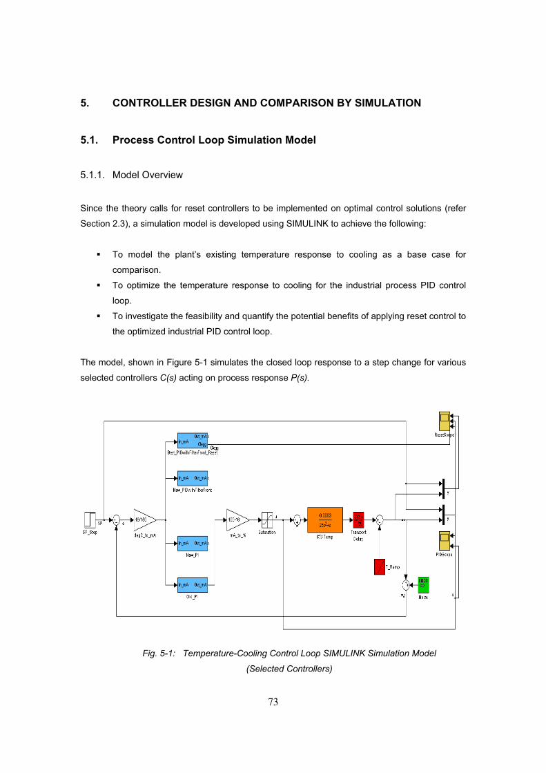
73
5. CONTROLLER DESIGN AND COMPARISON BY SIMULATION
5.1. Process Control Loop Simulation Model
5.1.1. Model Overview
Since the theory calls for reset controllers to be implemented on optimal control solutions (refer
Section 2.3), a simulation model is developed using SIMULINK to achieve the following:
To model the plant’s existing temperature response to cooling as a base case for
comparison.
To optimize the temperature response to cooling for the industrial process PID control
loop.
To investigate the feasibility and quantify the potential benefits of applying reset control to
the optimized industrial PID control loop.
The model, shown in Figure 5-1 simulates the closed loop response to a step change for various
selected controllers C(s) acting on process response P(s).
Fig. 5-1: Temperature-Cooling Control Loop SIMULINK Simulation Model
(Selected Controllers)

74
In Figure 5-1, the process response P(s) derived in Section 4 by means of performing open loop
step tests is highlighted in orange, with the associated transport delay separately in red. A
temperature ramp input, also highlighted in red, is included in the model to cater for the
temperature rate of change due to the exothermic nature of the process in this specific industrial
batch reactor (as opposed to a constant temperature batch reactor).
The design and simulation of certain individual controllers C(s) highlighted in blue is discussed in
detail in Sections 5.2 to 5.5, namely:
Existing PI control (“Old_PI”)
Improved linear PI control (“New_PI”)
Improved linear PI control with lead (“New_PIDwithFilterFront”) – similar to PID control
Reset control (“Best_PIDwithFilterFront_Reset”)
The SIMULINK simulation model (refer Figure 5-1) facilitates rigorous controller design and
tuning of the various controller options. A user-defined program called sCAD with Nyquist plot
functionality (developed by UCT Electrical Engineering Control Laboratory – M. Braae, 1999) is
used initially for the upfront analysis, design and optimization of the various controllers. The
optimized controllers are then validated with the SIMULINK model which emulates the actual
plant equipment with its absolute variable ranges and its anti-reset wind-up feature in order to
align it more closely to the actual plant PID algorithm.
The following points should be noted regarding the use of the two simulation tools, SIMULINK
versus sCAD, and the differences between them:
The SIMULINK model simulates the plant over its full range whereas sCAD assumes that
signals are defined relative to their operating points.
The SIMULINK model caters for reset wind-up by placing an extra saturation on the
integrator term of C(s) in addition to the overall limits on the plant input or CV stemming
from the actuator range of 0-100%. sCAD can simulate the loop with overall limits on the
plant input or CV (like SIMULINK) but does not cater for anti-reset wind-up.
The reset controller is a non-linear system that has nothing to do with Nyquist theory,
hence the SIMULINK model is necessary for its design and simulation which cannot be
done in sCAD. The reset controller is applied to the optimum linear system (namely
improved PI with lead, similar to PID), which must be built into the simulation model.

75
In order to quantify the benefits of reset control, all the controllers – namely existing PI,
improved linear PI, improved linear PI with lead and reset control – are required to be
modelled using the same simulator such that a comparison may be drawn.
In order to arrive at the final design for the selected four types of controllers shown in Figure 5-1,
a number of additional controller configurations are also tested and explored during the
development of the simulation model. These controller models, shown in Figure 5-2, are not
discussed in detail but are captured in Appendix 1 (PID controllers) and Appendix 2 (Reset
controllers). Larger and more legible landscape versions of Figure 5-1 and Figure 5-2 are
recorded in Appendix 3.
Fig. 5-2: Temperature-Cooling Control Loop SIMULINK Simulation Model
(All Controllers)
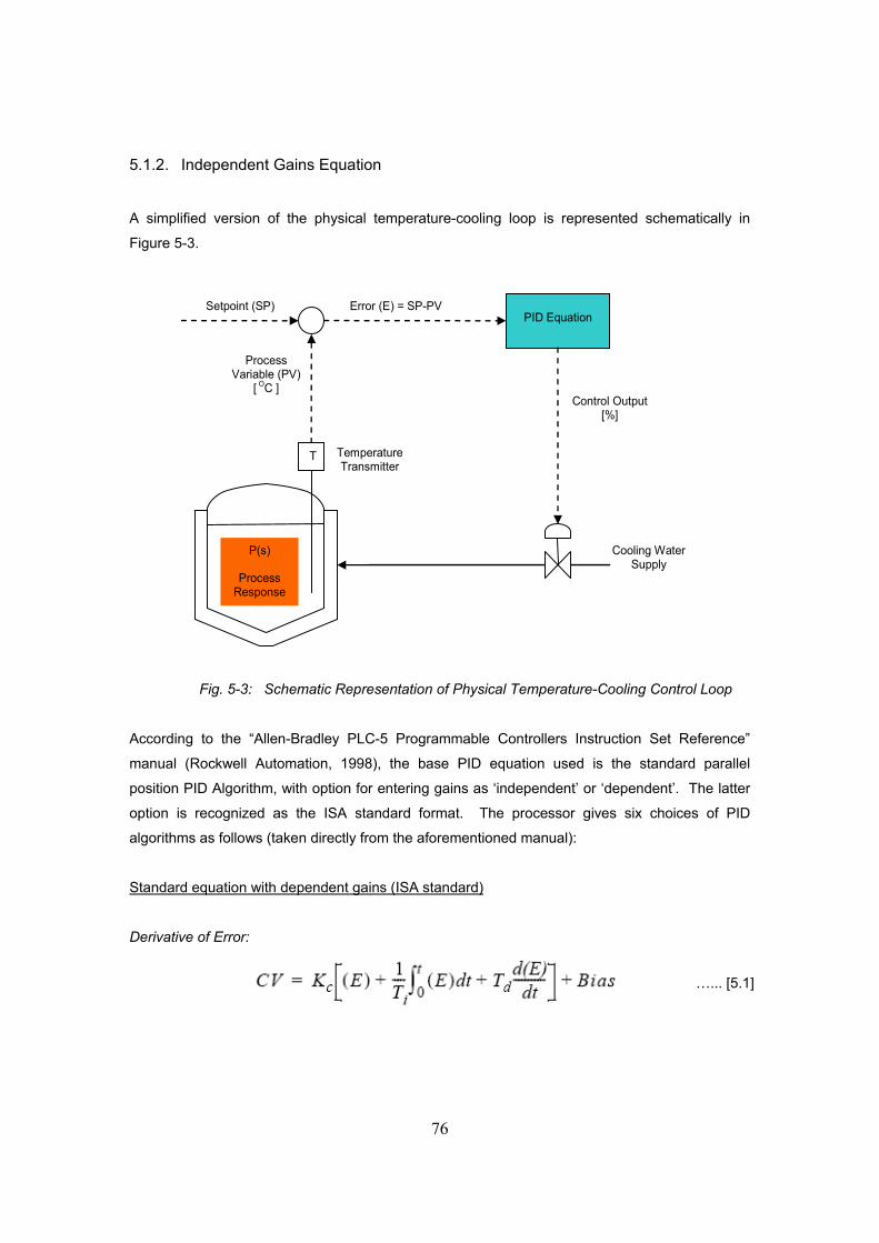
76
5.1.2. Independent Gains Equation
A simplified version of the physical temperature-cooling loop is represented schematically in
Figure 5-3.
Fig. 5-3: Schematic Representation of Physical Temperature-Cooling Control Loop
According to the “Allen-Bradley PLC-5 Programmable Controllers Instruction Set Reference”
manual (Rockwell Automation, 1998), the base PID equation used is the standard parallel
position PID Algorithm, with option for entering gains as ‘independent’ or ‘dependent’. The latter
option is recognized as the ISA standard format. The processor gives six choices of PID
algorithms as follows (taken directly from the aforementioned manual):
Standard equation with dependent gains (ISA standard)
Derivative of Error:
…... [5.1]
Temperature Transmitter
Control Output [%]
Setpoint (SP)
Process Variable (PV)
[ OC ]
Cooling Water Supply
PID Equation
P(s)
Process Response
Error (E) = SP-PV
T

77
Derivative of PV:
Independent gains equation
Derivative of Error:
Derivative of PV:
Where: CV = Output Control Variable (%)
Kc = Standard Controller Gain (unitless)
1/Ti = Reset Gain (repeats / minute)
Td = Rate Gain (repeats / minute)
Kp = Proportional Gain (unitless)
Ki = Integral Gain (seconds-1)
Kd = Derivative Gain (seconds)
E = Error = SP – PV or PV – SP (°C)
PV = Process Variable (°C)
SP = Setpoint (°C)
Bias = Feed-forward or External Bias
Note: One can convert from ‘standard’ to ‘independent’ gains constants by substituting
standard controller gain (Kc), reset gain (1/Ti) and rate gain (Td) values in the following
formulas:
...... [5.3]
...... [5.4]
...... [5.5]
...... [5.6]

78
Kp = Kc (unitless) …… [5.7]
Ki = Kc / (60.Ti) (seconds-1) …… [5.8]
Kd = Kc . (60.Td) (seconds) …… [5.9]
For the purposes of modeling the temperature-cooling water controller, it is important to
understand exactly which PID algorithm format is used. Therefore a thorough investigation into
the plant’s PLC code and settings reveals the existing parameters for the controller in question,
as summarized in Table 5-1.
Table 5-1: Existing Temperature-Cooling Water Control Parameter Settings
PLC Parameters
Temperature – Cooling Water
PID equation
Independent gains
Derivative of error .DOE
dPV / dt
Control action .CA
E = PV – SP
Kp (unitless)
Ki (seconds-1) Kd (seconds)
1
0.01 0
Loop update time .UPD (seconds)
5
PLC scan rate (ms)
300
Signal (mA)
4-20
Min temperature (°C) Max temperature (°C)
0
150
Min valve output (%) Max valve output (%)
0
100
As shown in Table 5-1, the temperature-cooling water PID controller makes use of the
Independent Gains equation with derivative of process variable (dPV / dt) and reverse control
action (E = PV – SP), refer equation [5.6] above.

79
Since derivative control is not applied in the existing controller (Kd = 0) – and in fact is rarely used
in any of the other controllers on the plant – the PID equation can be equated to the Independent
Gains equation with derivative of error (dE / dt) in this case, as shown by equation [5.4]. The
“dPV / dt” term simply caters for seamless control during setpoint changes made on-line, and
should not impact the model output in any event. Therefore equation [5.4] is the PID algorithm
format chosen for the simulation model shown in Figure 5-1 and 5-2.
In order to solve the complex mathematics of the PID algorithm during modelling, the time domain
PID equation [5.4] is converted to a Laplace transform in the s-domain. This gives rise to the
control transfer function C(s) defined below in [mA] / [mA] as used in the PLC.
Where: C(s) = Control Transfer Function (mA / mA)
Kp = Proportional Gain (unitless)
Ki = Integral Gain (seconds-1)
Kd = Derivative Gain (seconds)
5.1.3. Loop Update Time and PLC Scan Rate
In Table 5-1 it has been noted that in the PLC the loop update time has been set to 5 seconds for
the existing controller, while the PLC scan rate is 300 milliseconds for a cyclic task. Since four
separate cycles occur within the allocated 5-second loop update time, the total scan rate amounts
to 1200 milliseconds.
Generally, the selected scan rate must be at least 5 times larger than the required response time
of the controlled variable. Aggressive control action combined with a slow scan rate of the control
loop software will result in a stepped behaviour and ultimately in instability if the scan rate is
decreased further. Such stepped behaviour is an indication that the scan rate must be increased.
Since the Integral Gain Ki is time-based, this means that the actual integral action for the PID
controller is equal to 5/1.2 (approximately four) times larger than specified with the apparent
existing Ki settings. Similarly the actual derivative action for the PID controller is equal to 1.2/5
(approximately a quarter) of that specified with the apparent existing Kd. Therefore these scaling
factors are included in the modelling, as shown by equations [5.11] and [5.12] below, to ensure
the correct time-scale is used for the linear controller C(s) as in the existing PLC.

80
Real Ki = Ki × 5/1.2 (seconds-1) …... [5.11]
Real Kd = Kd × 1.2/5 (seconds) …... [5.12]
5.1.4. Engineering Scaling Factors
According to the “Allen-Bradley PLC-5 Programmable Controllers Instruction Set Reference”
manual (Rockwell Automation, 1998), the input and output range from 0-4095 (12-bit analogue)
and input scaling is in engineering units. As shown in Table 5-1, the plant makes use of a
4-20 mA signal (16 mA range) which in engineering units translates into a 0°C-150°C range in
temperature and a 0%-100% range in control valve position.
In the simulation model (refer Figure 5-1 and 5.2) the control models C(s) are defined in
[mA] / [mA] as used in the PLC (see equation [5.10]) hence engineering scaling factors are
included in the model to make C(s) compatible with the process response model P(s) whose units
are defined as [oC] / [%] (refer Section 4). The units of the controller must be inverse of those for
the given plant model P(s), namely [%] / [oC]. A simplified version of the existing PI closed loop
control diagram including engineering scaling factors (taken from Figure 5-1 and 5-2) is shown in
isolation in Figure 5-4.
Fig. 5-4: Temperature-Cooling Water Closed Loop Diagram Including Engineering
Scaling Factors
5.1.5. Valve Saturation
In practice the plant control valve output is saturated (limited) at 0% minimum and 100%
maximum limits. This effect is catered for in the SIMULINK model by defining these upper and
lower saturation limits in the “Saturation” function block (refer Figure 5-1 and 5-2), the detail of
which is shown in Figure 5-5.
P(s)
C(s)
Setpoint (SP)
[oC]
Error (E) = SP-PV
[oC] 16 mA 150oC
100% 16 mA
[mA]
[%]
[oC]
[oC]
[mA]
Process Variable
(PV)

81
Fig. 5-5: Saturation Function Block Detail Showing Definition of
Saturation Parameters for Cooling Water Valve
5.2. Existing PI Controller Base Case Simulation 5.2.1. Control Loop Analysis
The existing PI controller response for the temperature-cooling water process control loop is first
analysed theoretically using a Nyquist plot, and then simulated as a base case for comparison
with other possible controllers. Firstly, the existing control parameters for the current cooling water PI controller (see Table 5-1)
are used to define the transfer function of the linear controller C(s) in the existing process, namely
Kp = –1, Ki = –0.01 seconds-1 and Kd = 0 seconds (refer Section 5.1.2).
Negative gain constants are used in the equation and model because of the inverse relationship
between temperature and cooling water valve position – namely temperature decreases when the
cooling water valve opens and increases when it closes – that is manifested in a negative P(s)
process gain of –0.0003, in addition to accommodating the definition of Error E = SP – PV as
used by the simulation model shown in Figure 5-1 and 5-2.

82
As discussed in Section 5.1.3, scaling factors are included in the modelling to compensate for the
5-second loop update time and 300-millisecond PLC scan rate (see Table 5-1) thereby ensuring
the correct time-scale is used for the relevant gain constants and linear controller C(s), as per the
existing plant PLC (refer equations [5.11] and [5.12]):
Real Ki = –0.01 × 5/1.2 (seconds-1) …... [5.13]
Real Kd = 0 × 1.2/5 (seconds) …... [5.14]
The resulting control transfer function C(s) describing the existing temperature-cooling water PI
controller is as follows:
Where: C(s) = Existing PI Control Transfer Function (mA / mA)
Kp = Proportional Gain = – 1 (unitless)
Real Ki = Integral Gain = – 0.0417 (seconds-1)
Real Kd = Derivative Gain = 0 (seconds)
As shown in Figure 5-4 (refer Section 5.1.4), the existing PI control transfer function C(s) in
[mA] / [mA] (refer equation [5.15]) is multiplied together with the engineering scaling factors
[16mA] / [150oC] and [100%] / [16mA] which are included in the model to make C(s) compatible
with the process response model P(s) whose units are defined as [oC] / [%]. The resulting overall
controller model k(s) is defined as follows:
The controller model k(s) is then multiplied together with the process response model P(s) (refer
Section 4) to give the open loop model for the existing temperature-cooling water PI controller as
follows:

83
The Nyquist plot for the control loop (refer equation [5.17]) is shown in Figure 5-6. The open loop
contains no unstable poles and the plot encircles its critical point twice implying that the closed
loop is unstable with two unstable poles, and hence that the existing PI controller on the plant is
unstable.
Fig. 5-6: Nyquist Plot for Existing PI Controller Settings
Figure 5-7 shows the sCAD plots for the corresponding input (%) signal (see right-hand plot) and
closed loop output (oC) response (see left-hand plot) for the existing PI control loop. The output
response overshoots the temperature setpoint by 10oC in the first cycle, which is followed by
further cycling around the setpoint with increasing amplitude and no indication of settling. This
type of response is a typical reflection of instability, as concluded from the Nyquist plot (refer
Figure 5-6), which proves the existing PI control loop is unstable.
critical point
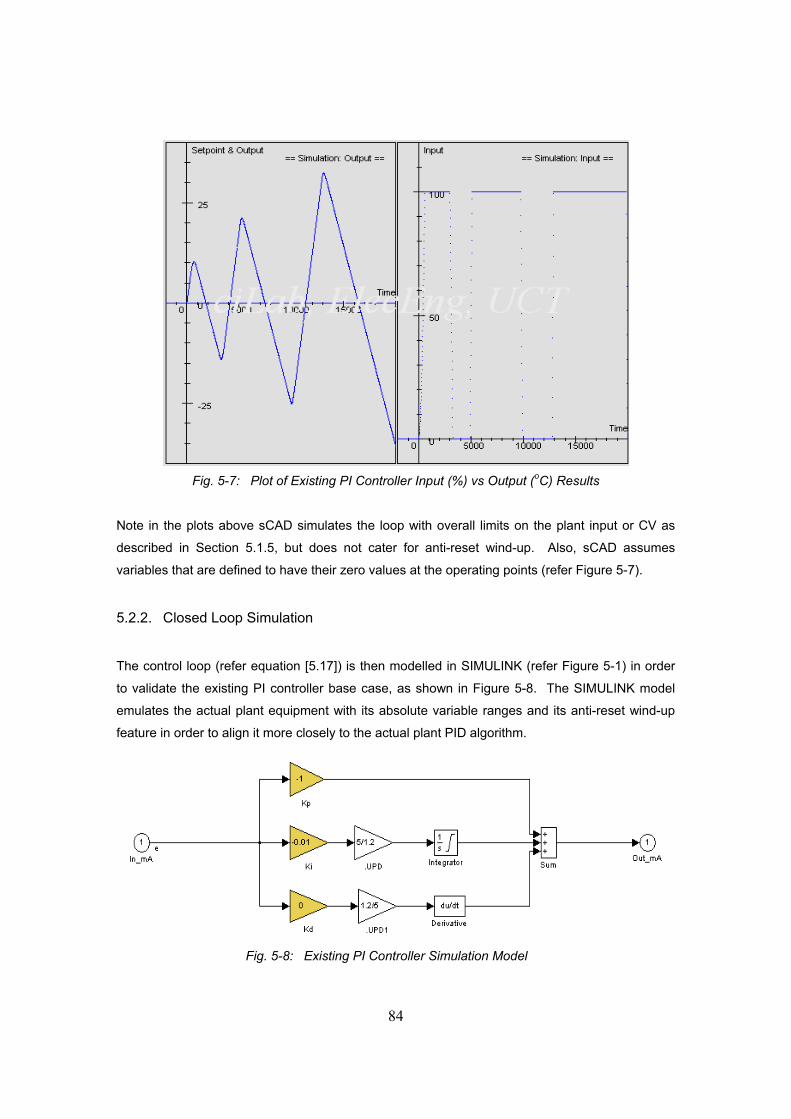
84
Fig. 5-7: Plot of Existing PI Controller Input (%) vs Output (oC) Results
Note in the plots above sCAD simulates the loop with overall limits on the plant input or CV as
described in Section 5.1.5, but does not cater for anti-reset wind-up. Also, sCAD assumes
variables that are defined to have their zero values at the operating points (refer Figure 5-7).
5.2.2. Closed Loop Simulation
The control loop (refer equation [5.17]) is then modelled in SIMULINK (refer Figure 5-1) in order
to validate the existing PI controller base case, as shown in Figure 5-8. The SIMULINK model
emulates the actual plant equipment with its absolute variable ranges and its anti-reset wind-up
feature in order to align it more closely to the actual plant PID algorithm.
Fig. 5-8: Existing PI Controller Simulation Model

85
Figure 5-8 represents the control transfer function C(s) in [mA] / [mA] for the existing PI control as
shown in Figure 5-4 (refer Section 5.1.4) and described by equation [5.15]. Section 5.2.1
describes in detail the source of the exact control parameters (Kp, Ki, Kd) and scaling factors
(5/1.2 and 1.2/5) shown in Figure 5-8 and used to derive C(s) (refer equation [5.15]).
In SIMULINK the simulation model includes an additional saturation on the integrator term to
cater for anti-reset wind-up in the plant PID control, thereby aligning it more closely to the actual
plant PID algorithm. Figure 5-9 shows how this is achieved by defining 0 mA lower and 16 mA
upper saturation limits in the 1/s “Integrator” function block. The 16 mA range emanates from the
use of a 4-20 mA signal on the plant (refer Table 5-1, Section 5.1.2). In addition to the saturation
for anti-reset wind-up the SIMULINK output is further limited to the actuator range of 0-100% as
discussed in Section 5.1.5 and shown in Figure 5-1 and 5-2.
Fig. 5-9: Integrator Function Block Detail Showing Selection of
Upper and Lower Saturation Limits
Figure 5-10 shows the results for the existing PI controller simulation of the closed loop response
with the time axis in seconds. The first graph (y) depicts the temperature response to a step
change in oC and the second graph (u) depicts the corresponding controller output in %.

86
The controller output in the simulation shows an oscillating temperature response with no
indication of settling and intermittent quenching of the cooling water valve which mimics on-off
control. The temperature overshoot in the simulation is 10oC.
Fig. 5-10: Existing PI Control Simulation (Base Case)
Note that in Figure 5-10 the SIMULINK model simulates the plant over its full absolute variable
ranges (namely the temperature coming up from 0oC and the actual setpoint at Tsp) whereas
sCAD assumes that signals are defined to have their zero values relative to their operating points
(refer Figure 5-7).
When comparing the two output response simulations of SIMULINK versus sCAD (refer Figures
5-10 and 5-7), one sees that the time axis for the SIMULINK simulation exhibits an offset
compared to the sCAD simulation. This is because the SIMULINK model is designed to mimic
the actual plant operation so the effect of the cooling water on temperature occurs only when the
temperature control loop kicks in – namely when the temperature crosses the setpoint – and
therefore the effect is zero for time t < 0. The point at which the control loop kicks in on the
SIMULINK model (t = 6000 seconds) corresponds to the time t = 0 on the sCAD plot.
In Figure 5-10, the simulation results for the existing PI control output show an oscillating
temperature response with no indication of settling, and intermittent quenching of the cooling
water valve which mimics on-off control. The temperature overshoot in the simulation is 10oC.
TSP
+10oC
-10oC

87
Figure 5-11 is a plot of actual plant data demonstrating the performance of the existing PI
controller. The on-off control action is a result of the tuning interaction combined with the
sequence-driven control within the specified temperature control band limits (refer Section 3.2
and 3.3). The simulation trend (Figure 5-10) correlates well with the actual plant data
(Figure 5-11) when comparing the period and amplitude of the two plots. In the first cycle, the
temperature overshoot is approximately 10oC in both cases, while the period of the response is
similar.
Fig. 5-11: Actual Plant Batch Data for Existing PI Control
During both the plant operation and in the SIMULINK model results (refer Figures 5-10 and 5-11)
the oscillatory nature of the control is evident. However, the instability typically denoted by
increasing amplitude of temperature response cycles – as seen in the sCAD simulation results
(refer Figure 5-7) – is masked by the fact that the cooling water valve output intermittently
saturates at its minimum and maximum limits of 0% and 100% respectively, which mimics on-off
control. In essence the instability becomes a so-called “limit cycle” in practice due to the
saturation of the plant signals (refer Figure 5-5). Both lag and lead times are present in a
temperature control loop of an exothermic reaction such as this batch dissolve process. This will
always lead to over- and under-shoot of the required limits with a dominant integral controller, and
oscillation is impossible to avoid.

88
When comparing the two output response simulations of SIMULINK versus sCAD (refer
Figures 5-10 and 5-7), one sees that the first temperature overshoot is approximately 10oC above
setpoint, which also correlates well with the trend observed on the plant (refer Figure 5-11).
During plant operation, the first temperature response cycle is considered a worst case scenario
since at this point the exothermicity and kinetics of the reaction is at its maximum for the relevant
batch and hence the temperature rate of change (or temperature ramp) is at its steepest (see
discussion in Section 2.2.1). Since the reaction kinetics of the process decreases with time, the
temperature ramp slows down as the batch proceeds, which in turn requires a less and less
aggressive control action. This phenomenon is evident when looking at the plant batch data
(refer Figure 5-11) which shows an oscillatory but decaying temperature response, with
corresponding decrease in each successive temperature overshoot and no maximum valve
saturation in the latter cycles. In this way – and in addition to the saturation limits placed on the
integrator – the batch process chemistry also prevents the existing PI controller from becoming
unstable on the actual plant.
In Section 5.2.1 Nyquist theory has been used in the sCAD program to prove the existing PI
controller settings are unstable (refer Figure 5-6). Through making use of both the sCAD and the
SIMULINK programs, one model is used to test another. The fact that both program models
concur in terms of the predicted output response – and also match the actual plant temperature
output trends – validates both simulation results and proves that the existing PI controller is
unstable.
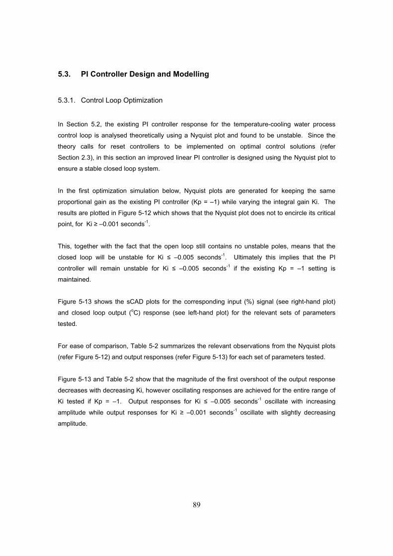
89
5.3. PI Controller Design and Modelling 5.3.1. Control Loop Optimization
In Section 5.2, the existing PI controller response for the temperature-cooling water process
control loop is analysed theoretically using a Nyquist plot and found to be unstable. Since the
theory calls for reset controllers to be implemented on optimal control solutions (refer
Section 2.3), in this section an improved linear PI controller is designed using the Nyquist plot to
ensure a stable closed loop system.
In the first optimization simulation below, Nyquist plots are generated for keeping the same
proportional gain as the existing PI controller (Kp = –1) while varying the integral gain Ki. The
results are plotted in Figure 5-12 which shows that the Nyquist plot does not to encircle its critical
point, for Ki ≥ –0.001 seconds-1.
This, together with the fact that the open loop still contains no unstable poles, means that the
closed loop will be unstable for Ki ≤ –0.005 seconds-1. Ultimately this implies that the PI
controller will remain unstable for Ki ≤ –0.005 seconds-1 if the existing Kp = –1 setting is
maintained.
Figure 5-13 shows the sCAD plots for the corresponding input (%) signal (see right-hand plot)
and closed loop output (oC) response (see left-hand plot) for the relevant sets of parameters
tested.
For ease of comparison, Table 5-2 summarizes the relevant observations from the Nyquist plots
(refer Figure 5-12) and output responses (refer Figure 5-13) for each set of parameters tested.
Figure 5-13 and Table 5-2 show that the magnitude of the first overshoot of the output response
decreases with decreasing Ki, however oscillating responses are achieved for the entire range of
Ki tested if Kp = –1. Output responses for Ki ≤ –0.005 seconds-1 oscillate with increasing
amplitude while output responses for Ki ≥ –0.001 seconds-1 oscillate with slightly decreasing
amplitude.

90
Fig. 5-12: Nyquist Plots for Linear PI Controller with Kp = –1 and Varying Ki
Fig. 5-13: Plot of Linear PI Controller Input (%) vs Output (oC) Results for
Kp = –1 and Varying Ki
Ki = -0.0001 s-1
Ki = -0.005 s-1
Ki = -0.001 s-1
Ki = -0.0005 s-1
Ki = -0.01 s-1
Ki = -0.1 s-1
Ki = -0.02 s-1
Ki = -0.0001 s-1
Ki = -0.0001 s-1Ki = -0.001 s-1
Ki = -0.001 s-1
Ki = -0.01 s-1
Ki = -0.1 s-1Ki = -0.01 s-1

91
Table 5-2: Linear PI Controller Optimization Results for Kp = –1 and Varying Ki
Kp
Ki
( s-1 )
Real Ki
( s-1 )
Kd
( s )
Real Kd
( s )
First
Over- Shoot ( oC )
Settling Time
( s )
Phase Margin
Damping Factor
Stable
–1
–0.0001
–0.000417
0
0
47.0
-
-
-
Yes
–1
–0.0005
–0.00208
0
0
27.5
-
-
-
Yes
–1
–0.001
–0.00417
0
0
22.0
-
-
-
Yes
–1
–0.005
–0.0208
0
0
12.5
-
-
-
No
–1
–0.01
–0.0417
0
0
11.0
-
-
-
No
–1
–0.02
–0.0833
0
0
8.0
-
-
-
No
–1
–0.1
–0.4177
0
0
6.0
-
-
-
No
In the second optimization simulation below, Nyquist plots are generated for keeping the same
integral gain as the existing PI controller (Ki = –0.01 seconds-1) while varying the proportional
gain Kp. The results are plotted in Figure 5-14 which shows that the Nyquist plot does not
encircle its critical point when –40 < Kp < –10. This, together with the fact that the open loop still
contains no unstable poles, implies that the closed loop is stable for Ki = –0.01 seconds-1 and
–40 < Kp < –10, and hence the PI control loop will also be stable at these controller settings.
However, both the phase margin and corresponding damping factor remain low, which means
that oscillation will appear in the system. For these stable control loops, both phase margin and
corresponding damping factor increase with decreasing Kp, thereby indicating that oscillations will
be reduced as Kp decreases. However, the Kp value cannot be decreased indefinitely since the
Nyquist plot shows that Kp values beyond –40 result in the critical point becoming encircled and
the control loop once again becoming unstable.
Figure 5-15 shows the sCAD plots for the corresponding input (%) signal (see right-hand plot)
and closed loop output (oC) response (see left-hand plot) for the relevant sets of parameters
tested.
For ease of comparison, Table 5-3 summarizes the relevant observations from the Nyquist plots
(refer Figure 5-14) and output responses (refer Figure 5-15) for each set of parameters tested.

92
Fig. 5-14: Nyquist Plots for Linear PI Controller with Ki = –0.01 seconds-1 and Varying Kp
Fig. 5-15: Plot of Linear PI Controller Input (%) vs Output (oC) Results for
Ki = –0.01 seconds-1and Varying Kp
Kp = -1
Kp = -10
Kp = -20
Kp = -40
Kp = -2
Kp = -0.5 Kp = -0.1
Kp = -15
Kp = -50
Kp = -30
Kp = -1
Kp = -10 Kp = -20
Kp = -40
Kp = -20
Kp = -0.1
Kp = -1
Kp = -40
Kp = -0.1 Kp = -10

93
Table 5-3: Linear PI Controller Optimization Results for Ki = –0.01 seconds-1 and Varying Kp
Kp
Ki
( s-1 )
Real Ki
( s-1 )
Kd
( s )
Real Kd
( s )
First
Over- Shoot ( oC )
Settling Time
( s )
Phase Margin
Damping Factor
Stable
–0.1
–0.01
–0.0417
0
0
11.0
-
-
-
No
–0.5
–0.01
–0.0417
0
0
11.0
-
-
-
No
–1
–0.01
–0.0417
0
0
10.5
-
-
-
No
–2
–0.01
–0.0417
0
0
10.0
-
-
-
No
–10
–0.01
–0.0417
0
0
7.5
-
-
-
No
–15
–0.01
–0.0417
0
0
7.5
18000
30o
0.30
Yes
–20
–0.01
–0.0417
0
0
6.5
8000
40o
0.40
Yes
–30
–0.01
–0.0417
0
0
5.5
9500
45o
0.45
Yes
–40
–0.01
–0.0417
0
0
5.0
-
-
-
No
–50
–0.01
–0.0417
0
0
5.0
-
-
-
No
From Figure 5-15, one can observe that –40 < Kp < –10 results in a decaying response that
eventually settles, indicating a stable control loop as concluded by the Nyquist plots. However,
as predicted, oscillation is present and this causes settling times to be excessive. Figure 5-15
shows that Kp ≤ –40 results in a response which oscillates at +/- 2oC around the setpoint,
indicating an unstable control loop as concluded by the Nyquist plot. Kp ≥ –10 results in an
oscillating response with increasing amplitude indicating an unstable control loop as concluded by
the Nyquist plots.
Figure 5-15 and Table 5-3 show that the magnitude of the first overshoot of the output response
decreases with decreasing Kp, regardless of whether or not the control loop is stable or unstable.

94
In the third optimization simulation below, since values for Kp < –10 appear to give a stable
closed loop response in the previous simulation (refer Figures 5-14 and 5-15, Table 5-3) Nyquist
plots are generated for keeping the proportional gain Kp = –10 constant while varying the integral
gain Ki. The results are plotted in Figure 5-16 which shows that the Nyquist plot does not encircle
its critical point when Ki > –0.01 seconds-1. This, together with the fact that the open loop still
contains no unstable poles, implies that the closed loop is stable for Kp = –10 and Ki > –0.01
seconds-1, and hence the PI controller will also be stable at these controller settings. For these
stable control loops, both phase margin and corresponding damping factor increase with
increasing Ki, thereby indicating that oscillations will be reduced as Ki increases.
Fig. 5-16: Nyquist Plots for Linear PI Controller with Kp = –10 with Varying Ki
Figure 5-17 shows the sCAD plots for the corresponding input (%) signal (see right-hand plot)
and closed loop output (oC) response (see left-hand plot) for the relevant sets of parameters
tested.
For ease of comparison, Table 5-4 summarizes the relevant observations from the Nyquist plots
(refer Figure 5-16) and output responses (refer Figure 5-17) for each set of parameters tested.
Ki = -0.0001 s-1
Ki = -0.0005 s-1
Ki = -0.001 s-1
Ki = -0.005 s-1
Ki = -0.01 s-1
Ki = -0.02 s-1
Ki = -0.1 s-1

95
Fig. 5-17: Plot of Linear PI Controller Input (%) vs Output (oC) Results for
Kp = –10 and Varying Ki
Table 5-4: Linear PI Controller Optimization Results for Kp = –10 and Varying Ki
Kp
Ki
( s-1 )
Real Ki
( s-1 )
Kd
( s )
Real Kd
( s )
First
Over- Shoot ( oC )
Settling Time
( s )
Phase Margin
Damping Factor
Stable
–10
–0.0001
–0.000417
0
0
10.2
∞
87o
0.87
Yes
–10
–0.0005
–0.00208
0
0
10.0
18000
85o
0.85
Yes
–10
–0.001
–0.00417
0
0
9.8
8000
75o
0.75
Yes
–10
–0.005
–0.0208
0
0
8.0
11000
30o
0.30
Yes
–10
–0.01
–0.0417
0
0
7.5
-
-
-
No
–10
–0.02
–0.0833
0
0
6.5
-
-
-
No
–10
–0.1
–0.4177
0
0
5.5
-
-
-
No
Ki = -0.0001 s-1
Ki = -0.0005 s-1
Ki = -0.001 s-1
Ki = -0.005 s-1
Ki = -0.01 s-1
Ki = -0.01 s-1
Ki = -0.1 s-1
Ki = -0.005 s-1
Ki = -0.001 s-1
Ki = -0.0005 s-1
Ki = -0.0001 s-1

96
From Figure 5-17, one can observe that –0.01 ≥ Ki ≥ –0.1 seconds-1 results in an oscillating
response with increasing amplitude, indicating an unstable control loop as concluded by the
Nyquist plots. Ki = –0.005 seconds-1 results in a decaying response that eventually settles,
indicating a stable control loop as concluded by the Nyquist plots. However, oscillations are
present and this causes settling time to be excessive. Ki ≥ –0.001 seconds-1 results in a stable
control loop with only one overshoot, as concluded by the Nyquist plots. For
Ki = –0.001 seconds-1, the phase margin of 75o and corresponding damping factor of 0.75 is a
substantial improvement compared to Ki = –0.005 seconds-1 where the phase margin is 30o and
corresponding damping factor is 0.3, indicating that oscillations in the systems will be reduced at
the higher value of Ki, as confirmed in Figure 5-17. This is also a significant improvement
compared to the previous simulations for Ki = –0.01 seconds-1 with higher Kp values (refer Figure
5-14 and Table 5-3).
As seen in Figure 5-17, although both phase margin and corresponding damping factor increase
with increasing Ki (thereby indicating that oscillations will be reduced) and the settling time
increases dramatically with increasing Ki for values beyond Ki = –0.001 seconds-1. The
magnitude of the first overshoot of the output response decreases slightly with decreasing Ki,
regardless of whether or not the control loop is stable or unstable.
In the final optimization simulation below, since Ki = –0.001 seconds-1 appears to give a stable
closed loop response with a good phase margin and associated damping factor in the previous
simulation, and therefore a response with an appropriate settling time and overshoot (refer
Figures 5-16 and 5-17, Table 5-4), Nyquist plots are generated for keeping the integral gain
Ki = –0.001 seconds-1 constant while varying the proportional gain Kp. The results are plotted in
Figure 5-18 which shows that the Nyquist plot does not encircle its critical point for values of
Kp > –50. This, together with the fact that the open loop still contains no unstable poles, implies
that the closed loop is stable for Ki = –0.001 seconds-1 and Kp > –50, and hence the PI control
loop will also be stable at these controller settings. For these stable control loops, both phase
margin and corresponding damping factor increase with decreasing Kp, thereby indicating that
oscillations will be reduced as Kp decreases. From the Nyquist plot, the control loop also appears
to become unstable for larger values of Kp ≥ –1, in addition to Kp ≤ –50.
Figure 5-19 shows the sCAD plots for the corresponding input (%) signal (see right-hand plot)
and closed loop output (oC) response (see left-hand plot) for the relevant sets of parameters
tested. For ease of comparison, Table 5-5 summarizes the relevant observations from the
Nyquist plots (refer Figure 5-18) and output responses (refer Figure 5-19) for each set of
parameters tested.

97
Fig. 5-18: Nyquist Plots for Linear PI Controller with Ki = –0.001 seconds-1 with Varying Kp
Fig. 5-19: Plot of Linear PI Controller Input (%) vs Output (oC) Results for
Ki = –0.001 seconds-1and Varying Kp
Kp = -1
Kp = -20
Kp = -50
Kp = -5
Kp = -9
Kp = -1
Kp = -20
Kp = -5
Kp = -9
Kp = -50
Kp = -1
Kp = -20
Kp = -5
Kp = -9
Kp = -50
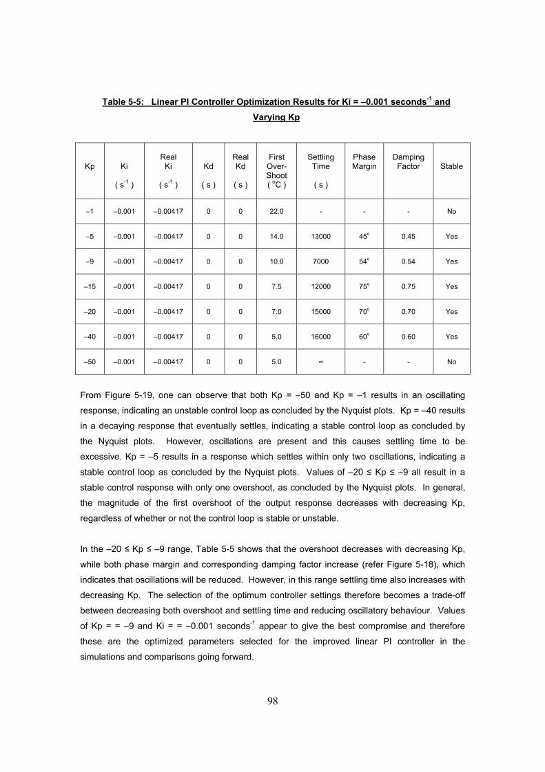
98
Table 5-5: Linear PI Controller Optimization Results for Ki = –0.001 seconds-1 and Varying Kp
Kp
Ki
( s-1 )
Real Ki
( s-1 )
Kd
( s )
Real Kd
( s )
First
Over- Shoot ( oC )
Settling Time
( s )
Phase Margin
Damping Factor
Stable
–1
–0.001
–0.00417
0
0
22.0
-
-
-
No
–5
–0.001
–0.00417
0
0
14.0
13000
45o
0.45
Yes
–9
–0.001
–0.00417
0
0
10.0
7000
54o
0.54
Yes
–15
–0.001
–0.00417
0
0
7.5
12000
75o
0.75
Yes
–20
–0.001
–0.00417
0
0
7.0
15000
70o
0.70
Yes
–40
–0.001
–0.00417
0
0
5.0
16000
60o
0.60
Yes
–50
–0.001
–0.00417
0
0
5.0
∞
-
-
No
From Figure 5-19, one can observe that both Kp = –50 and Kp = –1 results in an oscillating
response, indicating an unstable control loop as concluded by the Nyquist plots. Kp = –40 results
in a decaying response that eventually settles, indicating a stable control loop as concluded by
the Nyquist plots. However, oscillations are present and this causes settling time to be
excessive. Kp = –5 results in a response which settles within only two oscillations, indicating a
stable control loop as concluded by the Nyquist plots. Values of –20 ≤ Kp ≤ –9 all result in a
stable control response with only one overshoot, as concluded by the Nyquist plots. In general,
the magnitude of the first overshoot of the output response decreases with decreasing Kp,
regardless of whether or not the control loop is stable or unstable.
In the –20 ≤ Kp ≤ –9 range, Table 5-5 shows that the overshoot decreases with decreasing Kp,
while both phase margin and corresponding damping factor increase (refer Figure 5-18), which
indicates that oscillations will be reduced. However, in this range settling time also increases with
decreasing Kp. The selection of the optimum controller settings therefore becomes a trade-off
between decreasing both overshoot and settling time and reducing oscillatory behaviour. Values
of Kp = = –9 and Ki = = –0.001 seconds-1 appear to give the best compromise and therefore
these are the optimized parameters selected for the improved linear PI controller in the
simulations and comparisons going forward.

99
5.3.2. Control Loop Analysis
From the Nyquist plot analysis and PI parameter optimization exercise in Section 5.3.1, the
values of Kp = –9, Ki = –0.001 seconds-1 and Kd = 0 seconds give a good compromise between
minimizing both overshoot and settling time (refer Table 5-5), and the 10oC magnitude of
temperature overshoot also matches the existing plant data (refer Figure 5-11). For this reason
these values are chosen as the stable improved linear PI controller settings to define the new
transfer function of the linear controller C(s) for further analysis and simulation, and ultimately for
comparison with the existing PI controller base case (refer Section 5.2).
Negative gain constants are once again used in the equation and model because of the inverse
relationship between temperature and cooling water valve position – namely temperature
decreases when the cooling water valve opens and increases when it closes – that is manifested
in a negative P(s) process gain of –0.0003, in addition to accommodating the definition of Error
E = SP – PV as used by the simulation model shown in Figure 5-1 and 5-2.
As discussed in Section 5.1.3, scaling factors are once again included in the modelling to
compensate for the 5-second loop update time and 300-millisecond PLC scan rate (see
Table 5-1) thereby ensuring the correct time-scale is used for the relevant gain constants and
linear controller C(s), as used in the existing plant PLC (refer equations [5.11] and [5.12]):
Real Ki = –0.001 × 5/1.2 (seconds-1) …... [5.18]
Real Kd = 0 × 1.2/5 (seconds) …... [5.19]
The resulting control transfer function C(s) which describes the improved linear PI controller is as
follows:
Where: C(s) = Existing PI Control Transfer Function (mA / mA)
Kp = Proportional Gain = – 9 (unitless)
Real Ki = Integral Gain = – 0.00417 (seconds-1)
Real Kd = Derivative Gain = 0 (seconds)

100
As shown in Figure 5-4 (refer Section 5.1.4), the improved linear PI control transfer function C(s)
in [mA] / [mA] (refer equation [5.20]) is multiplied together with the engineering scaling factors
[16mA] / [150oC] and [100%] / [16mA] which are included in the model to make C(s) compatible
with the process response model P(s) whose units are defined as [oC] / [%]. The resulting overall
controller model k(s) is defined as follows:
The controller model k(s) is multiplied together with the process response model P(s) (refer
Section 4) to give the open loop model for the improved linear PI controller as follows:
The Nyquist plot for the improved linear PI control loop (refer equation [5.22]) is shown in
Figure 5-20, in comparison with the previous plot for the existing PI control (refer equation [5.17]).
Fig. 5-20: Nyquist Plots Comparing Existing PI and Improved Linear
PI Controller Settings
Existing PI (unstable)
Improved Linear PI (stable)
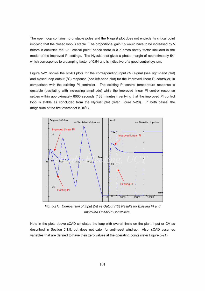
101
The open loop contains no unstable poles and the Nyquist plot does not encircle its critical point
implying that the closed loop is stable. The proportional gain Kp would have to be increased by 5
before it encircles the “–1” critical point, hence there is a 5 times safety factor included in the
model of the improved PI settings. The Nyquist plot gives a phase margin of approximately 54o
which corresponds to a damping factor of 0.54 and is indicative of a good control system.
Figure 5-21 shows the sCAD plots for the corresponding input (%) signal (see right-hand plot)
and closed loop output (oC) response (see left-hand plot) for the improved linear PI controller, in
comparison with the existing PI controller. The existing PI control temperature response is
unstable (oscillating with increasing amplitude) while the improved linear PI control response
settles within approximately 8000 seconds (133 minutes), verifying that the improved PI control
loop is stable as concluded from the Nyquist plot (refer Figure 5-20). In both cases, the
magnitude of the first overshoot is 10oC.
Fig. 5-21: Comparison of Input (%) vs Output (oC) Results for Existing PI and
Improved Linear PI Controllers
Note in the plots above sCAD simulates the loop with overall limits on the plant input or CV as
described in Section 5.1.5, but does not cater for anti-reset wind-up. Also, sCAD assumes
variables that are defined to have their zero values at the operating points (refer Figure 5-21).
Existing PI
Improved Linear PI
Improved Linear PI
Existing PI

102
5.3.3. Closed Loop Simulation
The control loop (refer equation [5.22]) is then modelled in SIMULINK (refer Figure 5-1) in order
to validate the improved linear PI controller, as shown in Figure 5-22. The SIMULINK model
emulates the actual plant equipment with its absolute variable ranges and its anti-reset wind-up
feature in order to align it more closely to the actual plant PID algorithm.
Figure 5-22 represents the control transfer function C(s) in [mA] / [mA] for the improved linear PI
control as shown in Figure 5-4 (refer Section 5.1.4) and described by equation [5.20].
Section 5.3.2 describes in detail the source of the exact control parameters (Kp, Ki, Kd) and
scaling factors (5/1.2 and 1.2/5) shown in Figure 5-22 and used to derive C(s) (refer equation
[5.20]). As discussed in Section 5.2.2, the SIMULINK simulation model includes an additional
“1/s” saturation on the integrator term to cater for anti-reset wind-up in the plant PID control. In
addition to the saturation for anti-reset wind-up the SIMULINK output is further limited to the
actuator range of 0-100% as discussed in Section 5.1.5 and shown in Figure 5-1 and 5-2.
Fig. 5-22: Improved Linear PI Controller Simulation Model
Figure 5-23 shows the results for the improved linear PI controller simulation of the closed loop
response with the time axis in seconds. The first graph (y) depicts the temperature response to a
step change in oC and the second graph (u) depicts the controller output in %.
Note that in Figure 5-23 the SIMULINK model simulates the plant over its full absolute variable
ranges (namely the temperature coming up from 0oC and the actual setpoint at Tsp) whereas
sCAD assumes that signals are defined to have their zero values relative to their operating points
(refer Figure 5-21).
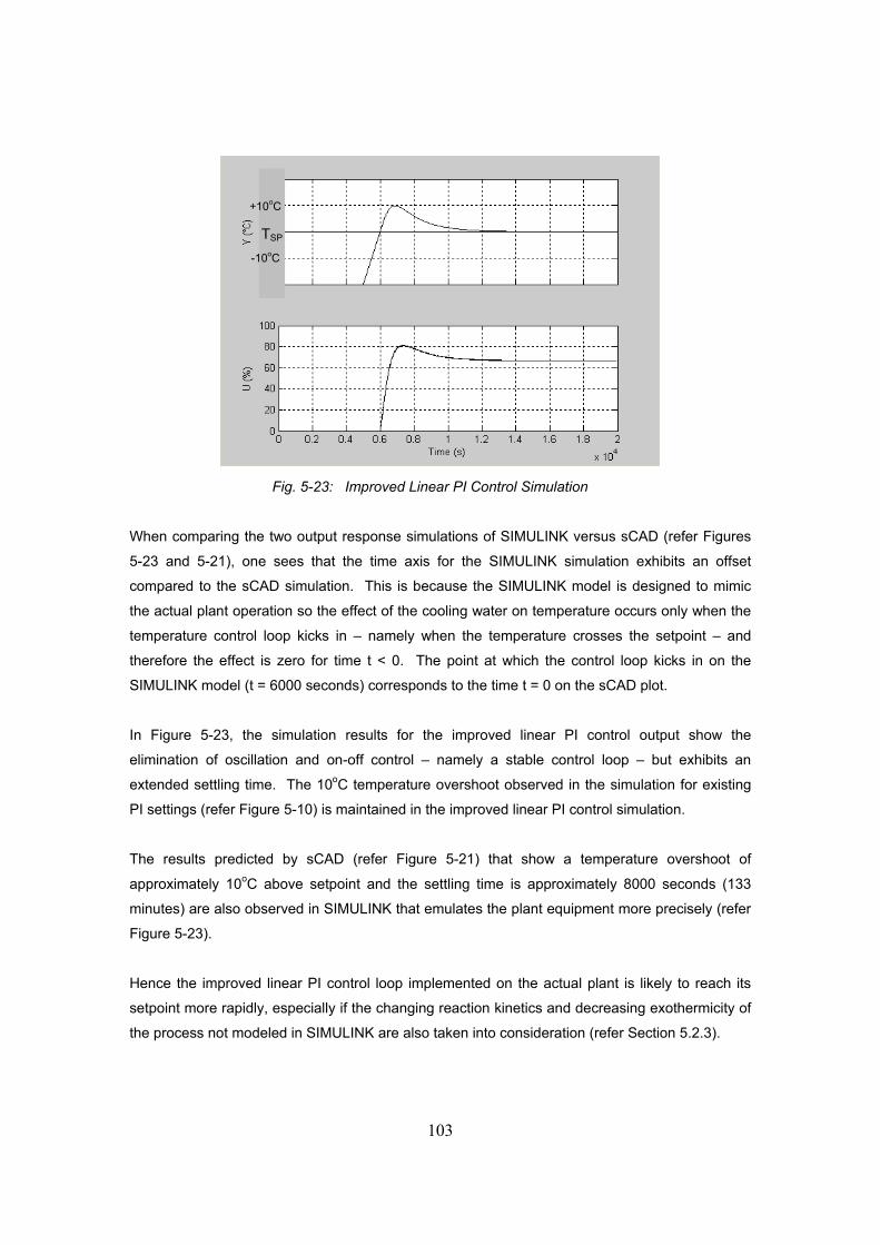
103
Fig. 5-23: Improved Linear PI Control Simulation
When comparing the two output response simulations of SIMULINK versus sCAD (refer Figures
5-23 and 5-21), one sees that the time axis for the SIMULINK simulation exhibits an offset
compared to the sCAD simulation. This is because the SIMULINK model is designed to mimic
the actual plant operation so the effect of the cooling water on temperature occurs only when the
temperature control loop kicks in – namely when the temperature crosses the setpoint – and
therefore the effect is zero for time t < 0. The point at which the control loop kicks in on the
SIMULINK model (t = 6000 seconds) corresponds to the time t = 0 on the sCAD plot.
In Figure 5-23, the simulation results for the improved linear PI control output show the
elimination of oscillation and on-off control – namely a stable control loop – but exhibits an
extended settling time. The 10oC temperature overshoot observed in the simulation for existing
PI settings (refer Figure 5-10) is maintained in the improved linear PI control simulation.
The results predicted by sCAD (refer Figure 5-21) that show a temperature overshoot of
approximately 10oC above setpoint and the settling time is approximately 8000 seconds (133
minutes) are also observed in SIMULINK that emulates the plant equipment more precisely (refer
Figure 5-23).
Hence the improved linear PI control loop implemented on the actual plant is likely to reach its
setpoint more rapidly, especially if the changing reaction kinetics and decreasing exothermicity of
the process not modeled in SIMULINK are also taken into consideration (refer Section 5.2.3).
TSP
+10oC
-10oC

104
5.4. PID Controller Design and Modelling 5.4.1. Control Loop Optimization
Since the theory calls for reset controllers to be implemented on optimal control solutions (refer
Section 2.3), in this section an attempt is made to further optimize the stable linear PI controller
designed in Section 5.3 through using the Nyquist plot to design an improved PID controller that
will possibly reduce overshoot and minimize settling time.
The Nyquist plot (Figure 5-20) indicates that the improved linear PI controller can be further
optimized by making the phase margin (and hence the damping factor of the control loop) larger,
thereby reducing the oscillation in the system. This is achieved by including a lead term, which is
similar to adding a derivative (D) term together with a first order filter.
Equation 5.10 (refer Section 5.1.2) gives a C(s) model that is non-causal and cannot be realized
in practice. However adding a filter to the derivative term makes the theoretical differential
feasible. In essence the model ‘s’ representing true differentiation is approximated by ‘s/(1+sT)’.
Appendix 1 shows a number of models tested in SIMULINK during the design and optimization of
the improved PID controller or linear PI with lead. Although the individual simulation results are
not discussed in any great depth, the models are used to determine the effect of using a simple
PID controller compared to one where first order filters and lead terms are placed in different
combinations at various points in the control loop (namely in front of the controller, behind the
controller and on the derivative term).
From the simulation exercise, the desired results are achieved by adding the first order filter
1/(1+50s) in front of the improved linear PI controller (developed in Section 5.3) which has
settings of Kp = –9 and Ki = –0.001 seconds-1, after which the derivative gain term (Kd) is further
optimized as shown in the Nyquist plot below.

105
Fig. 5-24: Nyquist Plots for Linear PI Controller with Lead where
Kp = –9, Ki = –0.001 seconds-1 and Varying Kd
Figure 5-24 shows that the Nyquist plot does not encircle its critical point for
Kd ≥ –18000 seconds in the range of Kd tested. This, together with the fact that the open loop
still contains no unstable poles, implies that the closed loop is stable for Kp = –9, Ki = –0.001
seconds-1 and Kd ≥ –18000 seconds, and hence the PI controller with lead will also be stable at
these controller settings. However, the control loop becomes unstable for much smaller values of
Kd, example Kd ≤ –90000 seconds. In the case of the stable control loops both phase margin
and corresponding damping factor increase slightly for Kp = –9, Ki = –0.001 seconds-1 and
decreasing Kd.
Figure 5-25 shows the sCAD plots for the corresponding input (%) signal (see right-hand plot)
and closed loop output (oC) response (see left-hand plot) for the relevant sets of parameters
tested.
For ease of comparison, Table 5-6 summarizes the relevant observations from the Nyquist plot
(refer Figure 5-24) and output responses (refer Figure 5-25) for each Kd parameter tested.
Kd = -9 s
Kd = -4500 s
Kd = -9000 s
Kd = -18000 s
Kd = -90000 s
Kd = -900 s

106
Fig. 5-25: Plot of Linear PI Controller with Lead Input (%) vs Output (oC) Results for
Kp = –9, Ki = –0.001 seconds-1 and Varying Kd
Table 5-6: Linear PI with Lead Controller Optimization Results for Ki = –9, Ki = –0.001 seconds-1 and Varying Kd
Kp
Ki
( s-1 )
Real Ki
( s-1 )
Kd
( s )
Real Kd
( s )
First
Over- Shoot ( oC )
Settling Time
( s )
Phase Margin
Damping Factor
Stable
–9
–0.001
–0.00417
–9
–2.16
67o
0.67
Yes
–9
–0.001
–0.00417
–900
–216
10.5
5500
67o
0.67
Yes
–9
–0.001
–0.00417
–4500
–1080
68o
0.68
Yes
–9
–0.001
–0.00417
–9000
–2160
8.5
6000
70o
0.7
Yes
–9
–0.001
–0.00417
–18000
–4320
7.5
10000
-
-
Yes
–9
–0.001
–0.00417
–90000
–21600
3.0
-
-
-
No
Kd = -9000 s
Kd = -18000 Kd = -90000
Kd = -900 s
Kd = -90000
Kd = -18000
Kd = -9000 s
Kd = -900 s

107
From Figure 5-25, Kd ≥ –9000 seconds results in a stable control response with only one
overshoot, as concluded by the Nyquist plots. Kd = –18000 seconds results a stable control
response, as concluded by the Nyquist plots, but with one overshoot and one undershoot and
hence a longer settling time. Kd = –90000 seconds results in an oscillating response, indicating
an unstable control loop as concluded by the Nyquist plots.
In general, the magnitude of the first overshoot of the output response decreases with decreasing
Kp, regardless of whether or not the control loop is stable or unstable.
Table 5-6 shows that for constant Kp = –9, Ki = –0.001 seconds-1, overshoot decreases while
settling time increases with decreasing values of Kd. Both phase margin and corresponding
damping factor are similar and high in value for the range of Kd ≥ –9000 seconds (refer
Figure 5-24), which indicates that oscillations are reduced in all these cases. Hence, although
the control loop is stable for this range of parameters tested, selection of the optimum controller
settings therefore becomes a trade-off between decreasing both overshoot and settling time.
Values of Kp = = –9 and Ki = = –0.001 seconds-1 and Kd = –9000 seconds appear to give the
best compromise and therefore these are the optimized parameters selected for the improved
linear PI controller with lead in the simulations and comparisons going forward.
5.4.2. Control Loop Analysis
From the Nyquist plot analysis and PID parameter optimization exercise in Section 5.4.1, the
values of Kp = –9, Ki = –0.001 seconds-1 and Kd = –9000 seconds together with a first order filter
1/(1+50s) gives a good compromise between minimizing both overshoot and settling time (refer
Table 5-6), and the 8.5oC magnitude of temperature overshoot is an improvement on the existing
plant data (refer Figure 5-11). For this reason these values are chosen as the stable improved
linear PI with lead controller settings to define the new transfer function of the linear controller
C(s) for further analysis and simulation, and ultimately for comparison with the existing PI
controller base case (refer Section 5.2) and improved linear PI controller (refer Section 5.3).
Negative gain constants are once again used in the equation and model because of the inverse
relationship between temperature and cooling water valve position – namely temperature
decreases when the cooling water valve opens and increases when it closes – that is manifested
in a negative P(s) process gain of –0.0003, in addition to accommodating the definition of Error
E = SP – PV as used by the simulation model shown in Figure 5-1 and 5-2.

108
As discussed in Section 5.1.3, scaling factors are once again included in the modelling to
compensate for the 5-second loop update time and 300-millisecond PLC scan rate (see
Table 5-1) thereby ensuring the correct time-scale is used for the relevant gain constants and
linear controller C(s), as used in the existing plant PLC (refer equations [5.11] and [5.12]):
Real Ki = –0.001 × 5/1.2 (seconds-1) …... [5.23]
Real Kd = –9000 × 1.2/5 (seconds) …... [5.24]
The resulting control transfer function C(s) which describes the improved linear PI controller with
lead – similar to a PID controller with a first order filter – is as follows:
Where: C(s) = Existing PI Control Transfer Function (mA / mA)
Kp = Proportional Gain = – 9 (unitless)
Real Ki = Integral Gain = – 0.00417 (seconds-1)
Real Kd = Derivative Gain = – 2160 (seconds)
Equation 5.10 (refer Section 5.1.2) gives a C(s) model that is non-causal and cannot be realized
in practice. However adding a filter to the derivative term makes the theoretical differential
feasible. In essence the model ‘s’ representing true differentiation is approximated by ‘s/(1+sT)’
that is achieved by adding the filter 1/(1+50s) in equation [5.25].
As shown in Figure 5-4 (refer Section 5.1.4), the improved linear PI control transfer function C(s)
in [mA] / [mA] (refer equation [5.25]) is multiplied together with the engineering scaling factors
[16mA] / [150oC] and [100%] / [16mA] which are included in the model to make C(s) compatible
with the process response model P(s) whose units are defined as [oC] / [%]. The resulting overall
controller model k(s) is defined as follows:

109
The controller model k(s) is multiplied together with the process response model P(s) (refer
Section 4) to give the open loop model for the improved linear PI controller with lead as follows:
The Nyquist plot for the resulting control loop (refer equation [5.27]) is shown in Figure 5-26, in
comparison with the previous plots for both the unstable existing PI controller (refer equation
[5.17]) and the stable improved linear PI controller (refer equation [5.22]).
Fig. 5-26: Nyquist Plots Comparing Existing PI, Improved Linear PI and Improved
Linear PI with Lead Controller Settings
The open loop contains no unstable poles and the Nyquist plot does not encircle its critical point
implying that the closed loop is still stable. The proportional gain Kp would have to be increased
by 5 before it encircles the “–1” critical point, hence there is a 5 times safety factor included in the
model of the improved PI settings. The Nyquist plot gives a phase margin of approximately 70o
which corresponds to a damping factor of 0.7 indicative of a good control system and an
improvement on the 54o phase margin and 0.54 damping factor results obtained for the
previously designed linear PI controller (refer Section 5.3).
Improved Linear PI with Lead
Existing PI (unstable)
Improved Linear PI (stable)

110
Figure 5-27 shows the sCAD plots for the corresponding input (%) signal (see right-hand plot)
and closed loop output (oC) response (see left-hand plot) when entering in the open loop model
(refer equation [5.27]) for the improved linear PI with lead controller. The output response
overshoots the temperature setpoint by 8.5oC and then settles within approximately
6000 seconds (100 minutes), verifying that the control loop is stable as concluded from the
Nyquist plot (refer Figure 5-26).
The improved linear PI with lead controller exhibits a 25% improvement in settling time and a
15% reduction in overshoot compared to the improved linear PI controller which is stable and
settles within 8000 seconds (133 minutes) with an overshoot 10oC.
Fig. 5-27: Comparison of Input (%) vs Output (oC) Results for Improved Linear PI
and Improved Linear PI with Lead Controllers
5.4.3. Closed Loop Simulation
The control loop (refer equation [5.27]) is then modelled in SIMULINK (refer Figure 5-1) in order
to validate the improved linear PI with lead controller, as shown in Figure 5-28. The SIMULINK
model emulates the actual plant equipment with its absolute variable ranges and its anti-reset
wind-up feature in order to align it more closely to the actual plant PID algorithm.
Improved Linear PI Improved Linear PI
Improved Linear PI with Lead
Improved Linear PI with Lead

111
Figure 5-28 represents the control transfer function C(s) in [mA] / [mA] for the improved linear PI
with lead control as shown in Figure 5-4 (refer Section 5.1.4) and described by equation [5.25].
Section 5.4.2 describes in detail the source of the exact control parameters (Kp, Ki, Kd) and
scaling factors (5/1.2 and 1.2/5) shown in Figure 5-28 and used to derive C(s) (refer equation
[5.25]). As discussed in Section 5.2.2, the SIMULINK simulation model includes an additional
“1/s” saturation on the integrator term to cater for anti-reset wind-up in the plant PID control. In
addition to the saturation for anti-reset wind-up the SIMULINK output is further limited to the
actuator range of 0-100% as discussed in Section 5.1.5 and shown in Figure 5-1 and 5-2.
Fig. 5-28: Improved Linear PI with Lead Controller Simulation Model
Figure 5-29 shows the results for the improved linear PI with lead controller simulation of the
closed loop response with the time axis in seconds. The first graph (y) depicts the temperature
response to a step change in oC and the second graph (u) depicts the controller output in %.
Note that in Figure 5-29 the SIMULINK model simulates the plant over its full absolute variable
ranges (namely the temperature coming up from 0oC and the actual setpoint at Tsp) whereas
sCAD assumes that signals are defined to have their zero values relative to their operating points
(refer Figure 5-27).

112
Fig. 5-29: Improved Linear PI Control with Lead Simulation
When comparing the two output response simulations of SIMULINK versus sCAD (refer
Figures 5-29 and 5-27), one sees that the time axis for the SIMULINK simulation exhibits an
offset compared to the sCAD simulation. This is because the SIMULINK model is designed to
mimic the actual plant operation so the effect of the cooling water on temperature occurs only
when the temperature control loop kicks in – namely when the temperature crosses the setpoint –
and therefore the effect is zero for time t < 0. The point at which the control loop kicks in on the
SIMULINK model (t = 6000 seconds) corresponds to the time t = 0 on the sCAD plot.
When comparing the SIMULINK simulations in Figure 5-29 with Figure 5-23, one can conclude
that the improved linear PI with lead controller performs marginally better than the improved linear
PI controller.
The results predicted by sCAD (refer Figure 5-27) that show a temperature overshoot of
approximately 8.5oC above setpoint and the settling time is approximately 6000 seconds
(100 minutes) are also observed in SIMULINK that emulates the plant equipment more precisely
(refer Figure 5-29). Hence the improved linear PI with lead control loop implemented on the
actual plant is likely to reach its setpoint more rapidly, especially if the changing reaction kinetics
and decreasing exothermicity of the process not modeled in SIMULINK are also taken into
consideration (refer Section 5.2.3).
At this point the temperature-cooling water PID control loop has been optimized as required for
the application of reset control.
TSP
+10oC
-10oC

113
5.5. Reset Controller Design and Modelling
5.5.1. Reset Controller Solution
The theory calls for reset controllers to be implemented on optimal control solutions. Now that
the linear control law has been designed and optimized, the reset control method described by
Beker et al (2004) can be applied to reduce overshoot. A reset controller (refer equation [2.14] in
Section 2.3) is designed for the batch reactor to test its effect on the temperature control loop.
Initially an attempt was made to apply the two-step reset controller design method shown in
Figure 2-17 (refer Section 2.3), which was used by Zheng et al (2000) and originally conceived by
Horowitz & Rosenbaum (1975). In this case the linear controller C(s) is first designed to meet all
control system specifications (as described in Sections 5-1 to 5-4), except for the overshoot
constraint, then the reset controller in the form of a first order reset element (FORE) is selected to
meet this overshoot specification. A SIMULINK model that implements the R-C(s)-P(s) structure
in which R is a FORE was tested, but showed that this structure does not do much for the initial
temperature overshoot since the PID controller only kicks in once the error has been zero (that is,
the reset does not do more than reset the zero back to a zero at the start of the control). Later on
when the reset action does kick in there are a number of reset-actions but the large overshoot in
the temperature response has already been and gone so this is unsuitable for the purposes of the
industrial reactor application.
Because of this aspect, the design of the reset controller had to revert to the alternate method
described by Beker et al (2004), refer Figure 2-11 in Section 2.3. However, in the case of the
reactor the whole controller (PI with lead) rather than a mere FORE circuit is taken to be the reset
control law, which is then modified to switch the integrator in the I-term of the PID controller.
As shown in Figure 5-30, the reset controller is modelled in SIMULINK (refer Figure 5-1 and 5-2)
by applying it to the optimized linear PI controller with lead (refer equation [5.25]), as described
above. The SIMULINK model emulates the actual plant equipment with its absolute variable
ranges and its anti-reset wind-up feature in order to align it more closely to the actual plant PID
algorithm. Alternative methods of modelling the reset controller in SIMULINK that are
investigated during design and optimization of the reset controller can be seen in Appendix 2.

114
Fig. 5-30: Reset Controller Simulation Model
Figure 5-30 represents the control transfer function C(s) in [mA] / [mA] for the improved linear PI
with lead control as shown in Figure 5-4 (refer Section 5.1.4) and described by equation [5.25],
but with a reset controller applied. Section 5.4.2 describes in detail the source of the exact
control parameters (Kp, Ki, Kd) and scaling factors (5/1.2 and 1.2/5) shown in Figure 5-30 and
used to derive C(s) (refer equation [5.25]).
As discussed in Section 5.2.2, the SIMULINK simulation model includes an additional “1/s”
saturation on the integrator term to cater for anti-reset wind-up in the plant PID control. In the
reset control simulation this 1/s saturation is maintained – similar to the simulation for the
improved linear PI control with lead (refer Figure 5-28) – but in this case it is renamed as the
“Reset_Integrator” function block which is connected to the reset functionality as shown in
Figure 5-30.
As per the linear PI and linear PI with lead simulations before, in addition to the saturation for
anti-reset wind-up the SIMULINK output is further limited to the actuator range of 0-100% as
discussed in Section 5.1.5 and shown in Figure 5-1 and 5-2.

115
Figure 5-31 shows the simulation of the closed loop response for the reset controller. The first
graph (y) depicts the temperature response to a step change in oC and the second graph (u)
depicts the controller output in %. As predicted from the reset control theory discussed in
Section 2.3, the reset controller simulation indicates a significant reduction in temperature
overshoot with rapid settling time.
Fig. 5-31: Reset Control Simulation
5.5.2. Non-zero Initial Conditions for Reset Control
In applying the modern theory of reset control to the industrial reactor the predominant theory was
found to assume a restrictive dynamic model for the plant; one in which the input has to be zero
to keep the output constant at a non-zero value. For the reset controller defined in Figure 5-30
the state of the Reset_Integrator cannot be reset to zero, as indicated by equation [2.14] in the
case described by Beker et al (2004). Instead it needs to take account of the value of the plant
input at the time of the reset switch and hence to apply a non-zero reset condition to the
Reset_Integrator when the error e(t) is zero.
Zheng et al (2000) describe a reset controller that sets the state variable, "x", to zero when the
error "e" is zero, and then equates the control variable "u" to the state variable. In other words,
although their plant, P, does not contain an integrating term explicitly, their reset controller does,
according to the paper, drop the control variable to zero when the error is zero. This in effect
forces the control variable to zero during the "reset" action, which is not allowed for in the reactor
control system.
TSP
+10oC
-10oC

116
However, the process followed by Zheng et al (2000) did not impose this non-zero restriction on
the plant model since although it does reset to zero they use a C(s) with an integrator. With
reference to Figure 2-17, note that if the block C(s) has the form of a PID controller or contains an
integrator, then the combination of P(s) and C(s) will have an integrator in it. This means that
block R can set its output to zero without difficulty since the plant input or control variable is
actually the output of C(s) and setting the input to C(s) to zero will not force the plant input (to P
from C) to zero. Therefore the case described in Zheng et al (2000) is unlike the "non-zero
requirement" imposed by the reset control configuration in Figure 5-30, and not allowed for on the
industrial plant.
In the case of Beker et al (2004), as well as other cases found in the literature (refer Section 2.3),
the theory of reset control also assumed that the plant input could be set to zero on reset, which
is unlike the "non-zero requirement" imposed by the reset control configuration in Figure 5-30,
and not allowed for on the industrial plant.
In the dissertation this limitation of the basic theory was modified to enable reset control for this
particular industrial process. In the literature actual industrial applications of reset control such as
this batch reactor appear to be scarce, and the incorporation of a non-zero initial condition for a
reset controller may well be unique.
As discussed in Section 5.2.2, in SIMULINK the simulation model includes an additional
saturation on the integrator term to cater for anti-reset wind-up in the plant PID control, thereby
aligning it more closely to the actual plant PID algorithm. Figure 5-9 shows how this is achieved
by defining 0 mA lower and 16 mA upper saturation limits in the 1/s “Integrator” function block,
where the 16 mA range emanates from the use of a 4-20 mA signal on the plant (refer Table 5-1,
Section 5.1.2). In comparison to the “Integrator” function block in Figure 5-9 which sets the initial
condition to zero, the “Reset_Integrator” function block must have a value assigned to the initial
condition when performing the simulation, as shown in Figure 5-32 below, in order to prevent the
occurrence of limit cycles.

117
Fig. 5-32: Reset_Integrator Function Block Detail Showing Programming
of Non-zero Initial Reset Condition
The specific value of the non-zero condition required appears to be linked to temperature rate of
change (ramp) by means of a linear relationship as shown in Figure 5-33.
Fig. 5-33: Relationship Between Temperature Ramp and Initial Reset Condition

118
Figure 5-34 shows a reset control simulation when using the zero initial reset condition, which
results in the appearance of limit cycles. In this case the first graph (y) depicts the temperature
response to a step change in oC and the second graph (u) depicts the controller output in %,
while the third graph (reset) shows the actual mA signal of the reset integrator alone.
Fig. 5-34: Reset Control Simulation:
(120s dead time, 0.020oC/s ramp, initial reset = zero)
Figures 5-35 to 5-37 demonstrates the reset control simulations for different temperature ramp
conditions dictating different reset control initial conditions and hence the initial control valve
settings. The non-zero initial reset condition results in the control valve “banging” open to a
certain initial output (%) when the temperature crosses the set-point.
In practice, the maximum temperature ramp (worst case scenario) occurs during the very first
oscillation when the most aggressive and exothermic reactions are taking place. Thereafter the
temperature ramp decreases gradually as the batch process proceeds and overall reaction
kinetics slow down, which may complicate implementation of the reset control.
Plant data shows a nominal ramp range of 0.020 – 0.030 oC/second while the simulations
indicate that the valve output saturates in the 0.025 – 0.030 oC/second ramp range. Process
operation at the top end of the nominal ramp range may therefore prove problematic.
TSP
+10oC

119
Fig. 5-35: Reset Control Simulation:
(120s dead time, 0.015oC/s ramp, initial reset = 7.8mA)
Fig. 5-36: Reset Control Simulation:
(120s dead time, 0.020oC/s ramp, initial reset = 10.6mA)
TSP
+10oC
TSP
+10oC

120
Fig. 5-37: Reset Control Simulation:
(120s dead time, 0.025oC/s ramp, initial reset = 13.4mA)
5.5.3. Reset Controller Sensitivity to Dead Time
Existing plant data reveals poor cooling water valve performance resulting in a 7-minute dead
time being observed, compared to the actual process dead time of 2 minutes confirmed by actual
plant step tests (refer Section 4). The simulations in Figures 5-38 to 5-39 demonstrate the effect
of this maximum observed dead time on the reset controller, which results in decreased settling
rate and severe temperature overshoot despite the valve saturating at 100% for long periods.
This is a typical example of a practical plant control problem, with the long dead time currently
having a similar detrimental effect on the existing PI control tuning and performance, as
demonstrated by the simulations for the optimized linear PI controller with lead (no reset control)
shown in Figures 5-40 to 5-41.
The increased dead time results in a 7°C (63%) and 5°C (38%) increase in temperature
overshoot for the reset and PI control simulations respectively. For reset control action to be
effective the valve will have to be repaired prior to implementation, or the reset control action
must kick in sooner to compensate for the long dead time. Valve performance deteriorating over
time may affect robustness of the reset controller.
TSP
+10oC

121
Fig. 5-38: Reset Control Simulation:
(120s dead time, 0.020oC/s ramp, initial reset = 10.6mA)
Fig. 5-39: Reset Control Simulation:
(450s dead time, 0.020oC/s ramp, initial reset = 10.6mA)
TSP
+10oC
-10oC
TSP
+10oC
-10oC

122
Fig. 5-40. Improved Linear PI with Lead Control Simulation:
(120s dead time, 0.020oC/s ramp)
Fig. 5-41. Improved Linear PI with Lead Control Simulation:
(450s dead time, 0.020oC/s ramp)
TSP
+10oC
-10oC
TSP
+10oC
-10oC

123
5.5.4. Reset Controller Sensitivity to Noise Disturbances
Although reset control appears to result in smaller overshoots than regular control schemes, this
does seem to be achieved at the expense of having much stronger changes in the manipulated
variable. This issue is typical of how the objective function to be minimized during model
predictive control usually includes a penalty term for excessive control and is one of the reasons
why minimum variance control is usually not used in practice. This characteristic may be
especially important if sensor noise is not negligible, hence the effect of sensor noise is also
investigated during the reset control simulations.
Ultimately, a conservative nominal value for noise in the temperature signal was determined from
actual plant data, which is applied in all the reset control simulations, as shown by the green
block in the simulation model in Figure 5-1 and 5-2. This nominal noise value of 0.02oC is
expected to produce a noise of 3-4% in the actuated variable. The effect of noise is
compensated for by optimizing the first order filter during the design of the optimized linear PI
controller with lead (see equation 5.25).
5.6. Controller Comparison and Evaluation by Simulation In order to quantify the benefits of implementing the various optimized controllers on the
temperature-cooling industrial process control loop, the existing PI control base case is compared
with simulations for improved linear PI control, improved linear PI control with lead (similar to PID
control) and reset control using the SIMULINK model shown in Figure 5-1.
Table 5.7 is a comparison of temperature overshoot and settling time for the different control
options depicted in Figures 5-10, 5-23, 5-29 and 5-31 respectively. There is a 15% reduction in
temperature overshoot and 25% improvement in settling time when comparing the improved
(stable) linear PI controller to the improved linear PI control with lead. Through application of
reset control the temperature overshoot is reduced by a further 53% and settling time by 67% as
compared to the improved linear PI control with lead, or a total of 60% reduction in temperature
overshoot and 75% reduction in settling time when comparing to the improved (stable) linear PI
control.

124
Table 5.7: Comparison of Temperature Overshoot and Settling Time for the Different Controllers
CONTROLLER
TEMPERATURE
OVERSHOOT
SETTLING
TIME
Existing PI 10.0oC unstable
Improved Linear PI 10.0oC 133 min
Improved Linear PI with Lead 8.5oC 100 min
Reset Control 4.0oC 33 min

125
6. CONCLUSION AND RECOMMENDATIONS The following conclusions can be drawn from the investigation and simulation of reset control
applied to the industrial batch reactor process:
1) The existing plant PI control loop is unstable, although the instability is masked on the
plant by the occurrence of on-off control action due to valve saturation, tuning interaction
with sequence-driven control between set temperature control band limits, as well as
decreasing exothermicity and kinetics of the process as the batch proceeds.
2) The existing temperature control can be stabilised and improved by re-designing the
existing parameter values of the PI control loop, however this will have no impact on the
current temperature overshoot.
3) Further improvement of temperature control in terms of reducing overshoot and
minimizing settling time through application of PI control with lead (similar to PID control)
is only marginal compared to stable PI control.
4) Reset control offers a significant improvement in reducing overshoot and minimising
settling time of the temperature control response compared to standard PI or PI control
with lead (similar to PID control). This result is consistent with the predictions of reset
control theory when applied to this particular industrial batch reactor.
5) A non-zero initial condition is required when applying reset control to this specific
industrial reactor process in order to prevent the occurrence of limit cycles. The specific
value of the non-zero condition has a linear relationship with temperature rate of change
(ramp) of the exothermic batch process. The simulations indicate that process operation
at the top end of the nominal temperature ramp range may well prove to be problematic
in practice if reset control is implemented on the industrial batch reactor. Also, the fact
that temperature ramp continually decreases with time due to the changing kinetics as
the batch proceeds may complicate the implementation of reset control on this industrial
reactor process.

126
6) The simulations show that an increased dead time has a detrimental effect on the
performance of the reset controller in terms of reducing temperature overshoot and
minimizing settling time. This aspect is likely to affect the robustness of the reset
controller if implemented on the industrial batch reactor. In practice, as observed with
this particular industrial batch process, the occurrence of an increased dead time is not
unlikely and could be caused by a variety of practical or maintenance issues such as, for
example, valve performance deteriorating over time due to wear.
7) The effect of noise is compensated for by optimizing the first order filter during the design
of the optimized linear PI controller with lead, and simulations show that it does not have
a negative effect on the performance of the reset controller at the nominal noise value of
+/-0.02oC experienced on the plant.
In practice, the success of reset control on this specific industrial batch reactor process is
impacted heavily by the various “on-plant” conditions, some of which the in-depth control study
has revealed. The following recommendations are made for the continued investigation of reset
control applied to this industrial batch reactor process with the intention of ultimately
implementing the reset controller in practice:
1) Step tests on a range of batches observed on the industrial plant, for example, with
differing compositions, size or volume and feed particle size – and at various stages
during these batches – are required to verify and refine the dynamic process model P(s).
A sensitivity analysis could be performed on the extra data.
2) The preliminary design and simulation of the linear PI, linear PI with lead and reset
controllers has been carried out for the cooling water – temperature control system.
Although this has established the method and shown promising results, the process
needs to be repeated with more batches of data in order to refine and substantiate the
models and simulation results for a range of batches observed on the industrial plant.
3) Further investigate the effect of changes in the temperature ramp on the dynamic
process model (more batches) and on reset control simulation (using different process
models) especially with respect to non-zero initial condition.
4) Perform a formal stability analysis of the reset control system since the present work
relies on digital simulation to check on stability.

127
In essence many simulations have been run that are closely aligned to the plant
operation and these provide an indication of stability for the case being considered.
However, stability is always critical and although a separate stability analysis based on
the models used in the simulation is unlikely to provide much additional insight into
stability, it would be more academic in nature. Since the controller is non-linear it would
require a Lyapunov stability analysis that is outside the scope of this MSc. Beker et al
(2004) suggest a possible topic for further research on reset control is to explore the use
of non-quadratic Lyapunov functions.
5) Beker et al (2004) recommend that another topic for future research is concerned with
the performance of reset control systems to sensor noise, where they would like to
evaluate the system gain from sensor noise to plant output. Although the effect of noise
on the reset control simulation was briefly explored in the investigation, this field of work
could be furthered with regards to the industrial plant application.
6) Use simulation to evaluate controller robustness including sensitivity to modelling errors
and the effect of disturbances that, for example, are due to changing batch
composition/size/volume and hence exothermicity, to fluctuating cooling water
temperature, to wearing or replacement of the control valve and the subsequent re-tuning
associated with these actions, and to unusual plant trips plus restarting of the plant.
Beker et al (2004) also recommend that robustness is an area of future research. They
mention that robustness of results with regards to hi-frequency parasitics is an open
issue and that generalizing this to a more general norm-bounded uncertain dynamic
would also be of interest.
7) Investigate how to program the filter for the PI control with lead in the plant PLC, and also
how to program or implement reset controller in practice on the industrial plant since
programming of these non-standard items in the existing PLC is not a straightforward
task. Beker et al (2004) also suggest that some other areas of future research should
include robustness, controller synthesis and performance limitations, where a formal
study of the performance limitations of reset control systems appears ripe and
challenging.
8) Lastly, Beker et al (2004) suggests that the boundaries defining the potential benefits and
cost for using reset control have yet to be drawn. The same applies in case of actual
implementation of reset control on the industrial reactor and further investigation is
required to define this.

128
LIST OF REFERENCES Allen Bradley (1998), “PLC-5 Programmable Controllers - Instruction Set Reference”, November
1998.
Amos, S. R. (1995). “Platinum Group Metal Dissolution Fundamentals”, MSc (Eng.) Thesis,
University of the Witwatersrand, Johannesburg, 1995.
Amos, S. (1997). “Fundamentals of the Silica Leach Process and FIC Dissolution Process”,
PMR Internal Teach-in Presentation by JMTC and Anglo Platinum Research Centre, Hex
River, Rustenburg, 20-21 November 1997.
Anglo Platinum (2006–2008). “Internal PMR Process Specific Information: Datasheets, P&IDs,
Work Instructions, Daily & Monthly Production Log Reports, Control Sequence Code, Raw
Data”, Anglo Platinum, 2006–2008.
Anglo Platinum Research Centre & JMTC (2007). “PGM Refining Course: Various Course Notes
and Presentation Slides”, Anglo Platinum, Rustenburg, 2007.
Asamoah-Bekoe, Y. (1998). “Investigation of the Leaching of the Platinum Group Metal
Concentrate in Hydrochloric Acid Solution by Chlorine“, MSc (Eng.) Thesis, University of the
Witwatersrand, Johannesburg, March 1998.
Beker, O., Hollot, C. V. & Chait, Y. (2001a). “Plant with Integrator: An Example of Reset Control
Overcoming Limitations of Linear Feedback”, IEEE Transactions on Automatic Control,
46(11), November 2001, pp.1797–1799.
Beker, O., Hollot, C. V. & Chait, Y. (2001b). “Stability of Limit Cycles in Reset Control Systems”,
Proceedings of the 2001 American Control Conference, Arlington, VA, June 2001, pp.4681–
4682.
Beker, O., Hollot, C. V. & Chait, Y. (1999). “Stability of a Reset Control System Under Constant
Inputs”, Proceedings of the American Control Conference, San Diego, CA, June 1999,
pp.3044–3045.
Beker, O., Hollot, C. V., Chait, Y. & Han, H. (2004). “Fundamental Properties of Reset Control
Systems”, Automatica, 40, pp.906–915.
129
Bobrow, J. E., Jabbari, F. & Thai, K. (1995). “An Active Truss Element and Control Law for
Vibration Suppression”, Smart Materials Structures, 4, 1995, pp.264–269.
Bouhenchir, H., Cabassud, M. & Lann, M. V. (2006). “Predictive Functional Control for the
Temperature Control of a Chemical Batch Reactor”, Computers & Chemical Engineering,
Vol., 30, pp 1141–1154, 2006.
Branicky, M. S. (1998). “Multiple Lyupanov Functions and Other Analysis Tools for Switched and
Hybrid Systems”, IEEE Transactions on Automatic Control, 43, 1998, pp.475–482.
Bupp, R. T., Bernstein, D. S., Chellaboina, V. S. & Haddad, W. M. (2000). “Resetting Virtual
Absorbers for Vibration Control”, Journal of Vibration and Control, 6, 2000, pp.61–83.
Burnham, R. F. & Grant, R. A. (1999). “High Intensity Dissolution and Feed Preparation: Position
Paper Summarizing Key Results and Current Status”, JMTC Internal Report, JMTC, May
1999.
Burnham, R.F., Grant, R. A. & Smith, A. (2000). “High Intensity Dissolution and Feed Preparation:
Presentation Notes”, Internal Presentation by R. Grant at PMR, JMTC, June 2000.
Burnham, R. F., Grant R. A., Leinonen, S., Smith, A. J. & Woodman, D. (2004). “High Intensity
Dissolution of PMR Feeds”, JMTC Internal Final Report, JMTC, April 2004.
Chen, Q., Chait, Y. & Hollot, C. V. (2001). “Analysis of Reset Control Systems Consisting of a
FORE and Second Order Loop”, ASME Journal of Dynamic systems, Measurement and
Control, 123, June 2001, pp.279–283.
Chen, Q., Hollot, C. V. & Chait, Y. (2000). “Stability and Asymptotic Performance Analysis of
Reset Control Systems”, Proceedings of the 39th IEEE Conference on Decision and Control,
Sydney, Australia, December 2000, pp.251–256.
Clegg, J. C. (1958). “A Nonlinear Integrator for Servomechanisms”, Transactions A.I.E.E., 77 (Part II), March 1958, pp.41–42.
DeCarlo, R. A., Zak, S. H. & Matthews, G. P. (1988). “Variable Structure Control of Nonlinear
Multivariable Systems: A Tutorial”, IEEE Proceedings, 76(3), 1988, pp.212–232.

130
Edgar, T. F. (2004). “Control and Operations: When Does Controllability Equal Profitability?”,
Computers & Chemical Engineering, Vol. 29, pp 41–49, 2004.Beker, O., Hollot, C. V. & Chait,
Y. (2000). “Forced Oscillations in Reset Control Systems”, Proceedings of the 39th IEEE
Conference on Decision and Control, Sydney, Australia, December 2000, pp.4825–4826.
Feuer, A., Goodwin, G. C. & Salgado, M. (1997). “Potential Benefits of Hybrid Control for Linear
Time Invariant Plants”, Proceedings of the American Control Conference, Albuqueque, June
1997, pp.2790–2794.
Fileti, A. M. F., Antunes, A. J. B., Silva, F. V., Silveira, V. & Pereira, J.A.F.R., (2007).
“Experimental Investigations on Fuzzy Logic for Process Control”; Control Engineering
Practice, Vol. 15(1), 1149–1160.
Friedrich, M. & Perne, R. (1995). “Design and control of batch reactors – An industrial Viewpoint”
Computers & Chemical Engineering, Vol. 19, 357 – 368.
Goldberg, R. N. & Hepler, L. G., (1968). “Thermochemistry and Oxidation Potentials of the
Platinum Group Metals and Their Compounds”, Chemical Reviews Publication, Vol. 68, No.
2, 1968, pp.229–252.
Grant, R. A. (2000a). “High Intensity Dissolution Presentation”, PMR Internal Refining
Conference, Anglo Platinum, Rustenburg, September 2000.
Grant, R. A. (2000b). “Update on the Generation of Acid During High Intensity Dissolution”, PMR
Internal Memorandum to H. Scriba, Anglo Platinum, 12 April 2000.
Grant, R. A. (2003). “Report on Technical Review of Precious Metals Refiners: SOLVEX Core”,
PMR Internal Report, JMTC, August 2003.
Haddad, W. M., Chellaboina, V. & Kablar, N. A. (2000). “Active Control of Combustion Instabilities
via Hybrid Resetting Controllers”, Proceedings of the American Control Conference, Chicago,
IL, June 2000, pp.2378–2382.
Haddad, W. M., Chellaboina, V. & Kablar, N. A. (1999). “Nonlinear Impulsive Dynamical Systems
Part I: Stability and Dissipativity”, Proceedings of Conference on Decision and Control,
Phoenix, AZ, pp.4404-4422.

131
Hollot, C. V., Zheng, Y. & Chait, Y. (1997). “Stability Analysis for Control Systems with Reset
Integrators”, Proceedings of the 36th IEEE Conference on Decision and Control, San Diego,
CA, December 1997, pp.1717–1719.
Horowitz, I. & Rosenbaum, P. (1975). “Non-linear Design for Cost of Feedback Reduction in
Systems with Large Parameter Uncertainty”, International Journal of Control, 24(6), pp.997–
1001.
Hu, H., Zheng, Y., Chait, Y. & Hollot, C. V. (1997). “On the Zero-Input Stability of Control Systems
with Clegg Integrators”, Proceedings of the 1997 American Control Conference, Albuquerque,
NM, June 1997, pp.408–410.
Hu, H., Zheng, Y., Chait, Y. & Hollot, C. V. (1999). “On the Stability of Control Systems Having
Clegg Integrators”, In D. E. Miller & Li Qiu (Editors.), Topics in Control and its Applications – a
Tribute to Edward J. Davidson, Springer, Berlin, pp.107–115.
Keshav, P. (2005). “An Investigation into the High Intensity Dissolve Process”, PMR Internal
Report, Anglo Platinum, December 2005.
Kogel, P. (2002). “Pressure Dissolve Reactor Commissioning Report”, PMR Internal Report,
Anglo Platinum, February 2002.
Krishnan, K. R. & Horowitz, I. M. (1974). “Synthesis of a Non-linear Feedback System with
Significant Plant-ignorance for Prescribed System Tolerances”, International Journal of
Control, 19(4), pp.689–706.
Kyffin, D. (2003). “PMR Technical Review: RM and FC Dissolve”, PMR Internal Report, Anglo
Platinum, August 2003.
Lahee, R. (2006). “Control of a Batch Reactor in the Precious Group Metals Industry”,
Proceedings of the SACAC Control Conference, Durban, South Africa, 6–7 July 2006, pp.97,
120–128.
Lahee, R. (2007). “Application of Reset Control to a Batch Reactor in the Precious Group Metals
Industry”, Proceedings of the 7th IFAC Symposium of Nonlinear Control Systems, Pretoria,
South Africa, 21–24 August 2007, pp.97, 1080–1085.

132
Lahee, R. (2005a). “PMR Control Study Workshop Summary”, Anglo Platinum Management
Services Internal Report, Anglo Platinum, 14 April 2005.
Lahee, R. (2004). “Proposed PMR Primary Dissolve Controllability Audit”, Anglo Platinum
Management Services Internal Memo, Anglo Platinum, 11 November 2004.
Lahee, R. (2005b). “Process Control Audit: PMR Primary Dissolve”, Anglo Platinum Management
Services Internal Report, Anglo Platinum, 13 January 2005.
Lahee, R. (2006a). “Process Control Study: Control System Design Strategy Flowchart” Rev. 0,
Anglo Platinum Management Services Internal Report, Anglo Platinum, 21 February 2006.
Lahee, R. (2006b). “Process Control Study: General Procedure”, Anglo Platinum Management
Services Internal Report, Anglo Platinum, 2006.
Lau, K. & Middleton, R. (2000). “On the Use of Switching Control for Systems with Bounded
Disturbances”, Proceedings of the 39th IEEE Conference on Decision and Control, Sydney,
Australia, December 2000.
Lombard, N. F. (2005a). “Controller Configuration Guide”, Rev. 2a, Anglo Platinum Management
Services Internal Report, Anglo Platinum, 31 January 2005.
Lombard, N. F. (2005b). “PMR Primary Dissolve and SX Regulatory Control Assessment”, Rev.
a, Anglo Platinum Management Services Internal Report, Anglo Platinum, 28 January 2005.
Lombard, N. F. (2005c). “PMR Regulatory Control Workshop Presentation”, Slides from Anglo
Platinum Management Services Internal Presentation to PMR, Anglo Platinum, 6 May 2005.
Nagy, Z. & Agachi, S. (1997), “Model Predictive Control of a PVC Batch Reactor; Computers &
Chemical Engineering, Vol. 21(6), 571–591.
Scriba, H. (2000). “Motivation for Installation of High Intensity Dissolve”, PMR Internal
Memorandum, Anglo Platinum, 17 March 2000.
Scriba, H. (2000a). “HID Project Process Description”, PMR Internal Design Document, Anglo
Platinum, 2000.

133
Scriba, H. (2000b). “HID Project Process Design Basis”, PMR Internal Design Document, Anglo
Platinum, 2000.
Singer, N. C. & Seering, W. P. (1990). “Preshaping Command Inputs to Reduce System
Vibration”, Transactions of the ASME, 112, March 1990, pp.76–82.
Tsypkin, Y. Z. (1984). “Relay Control Systems”, Cambridge University Press, Cambridge.
Venter, R. (2000). “High Intensity Dissolution Project: Pressure Dissolve Reactor Commissioning
Report”, PMR Internal Report, Anglo Platinum, 6 September 2000.
Venter, R. & Muller, H. (2001). “High Intensity Dissolution Project”, Paper written for Anglo
American Symposium, Anglo Platinum Management Services, 2001.
Venter, R. (2004). “PMR Global Control Philosophy: General Specifications”, Rev.1, Anglo
Platinum Management Services Internal Document, Anglo Platinum, 31 March 2004.
Yamamguchi, T. (1997). “A Mode-switching Controller with Initial Value Compensation for Hard
Disk Drive Servo Control”, Control Engineering Practice, 5(11), pp.1525-1532.
Ye, H., Michel, A. N. & Hou, L. (1998). “Stability Analysis of Systems with Impulse Effects”, IEEE
Transactions on Automatic Control, 43(12), December 1998, pp.1719–1723.
Zheng, Y., Chait, Y., Hollot, C. V., Steinbuch, M. & Norg. M. (2000). “Experimental Demonstration
of Reset Control Design”, Control Engineering Practice, 8(2), pp.113–120.

134
APPENDIX

135
Appendix 1:
Other SIMULINK Models Investigated During the Design and Simulation
of the Improved PID or Linear PI with Lead Controller.
Appendix 1 describes the progressive testing of various controller model options during the
design and simulation of the improved PID controller and improved linear PI control with lead
(similar to PID), with positioning of filters in various places (refer Section 5.4). The integration of
these particular control transfer functions C(s) within the overall temperature-cooling control loop
SIMULINK simulation model is shown in Figure A3-2 (refer Appendix 3), which is also fully
discussed in Section 5.1. In all the models below, the initial control transfer function C(s) to which
filters and lead terms are then added is defined by equation 5.10 (refer Section 5.1.2):
Where: C(s) = Control Transfer Function (mA / mA)
Kp = Proportional Gain (unitless)
Ki = Integral Gain (seconds-1)
Kd = Derivative Gain (seconds)
In the first instance, an attempt is made to design an improved PID controller through simply
adding a derivative gain (Kd) setting to the existing PI controller where Kp = –1 and
Ki = –0.01 seconds-1, and then attempting to optimize the Kd. The resulting SIMULINK model is
shown in Figure A1-1, with Kd = –660 seconds.
Fig. A1-1: SIMULINK Model for Controller Settings of “Old_PIwithD”

136
Secondly, an attempt is made to optimize both the proportional gain (Kp) and derivative gain (Kd)
settings simultaneously while maintaining the existing Ki = –0.01 seconds-1 setting. The resulting
SIMULINK model is shown in Figure A1-2, with Kp = –35.72 and Kd = –22000 seconds.
Fig. A1-2: SIMULINK Model for Controller Settings of “New_PIwithD”
The model for the control transfer functions C(s) represented in Figure A1-1 and A1-2 are
described by Equation 5.10 (refer Section 5.1.2) which gives a C(s) model that is non-causal and
cannot be realized in practice. However adding a filter to the derivative term makes the
theoretical differential feasible. In essence the model ‘s’ representing true differentiation is
approximated by ‘s/(1+sT)’. Therefore the next step is to investigate the design of PID controllers
with filters or lead terms added in various places.
Figure A1-3 shows a PID controller with first order filter 1/(1+60s) added to the derivative (D) term
while maintaining the controller gain settings of Kp = –35.72, Ki = –0.01 seconds-1 and
Kd = –22000 seconds optimized in Figure A1-2.
Figure A1-4 shows a PID controller with first order filter 1/(1+60s) added at the back end of the
controller while maintaining the controller gain settings of Kp = –35.72, Ki = –0.01 seconds-1 and
Kd = –22000 seconds optimized in Figure A1-2.

137
Fig. A1-3: SIMULINK Model for Controller Settings of New_PIDwithFilterD”
Fig. A1-4: SIMULINK Model for Controller Settings of “New_PIDwithFilterBack”
Figure A1-5 shows subsequent experimentation with adapting the integral gain to
Ki = –0.001 seconds-1 and adding a linear lead term (500s+1)/(50s+1) at the back end of the
controller, then optimizing the controller gain settings to Kp = –8.3 and Kd = –1 seconds.

138
Fig. A1-5: SIMULINK Model for Controller Settings of “New_PIwithLead”
Figure A1-6 shows the next controller model tested which maintains the integral gain of
Ki = –0.001 seconds-1 while optimizing the proportional gain (Kp) and derivative gain (Kd) settings
with various first order filters placed both in front of the controller and on the derivative (D) term.
The resulting combination of first order filters is optimized to 1/(150s+1) in front and 1/(15s+1) on
the D-term respectively, acting together with the final optimized values of Kp = –9 and
Kd = –9000 seconds.
Fig. A1-6: SIMULINK Model for Controller Settings of “New_PIDwithFilterBoth”

139
Finally, Figure A1-7 shows the last controller model tested which maintains the Kp = –9,
Ki = –0.001 seconds-1 and Kd = –9000 seconds settings with optimized first order filter 1/(50s+1)
alone in front of the controller, and this time excludes the filter on the derivative (D) term. This
optimized version of the improved linear PI controller with lead (similar to PID) forms the basis of
the detailed analysis and discussion in Section 5.4.
Fig. A1-7: SIMULINK Model for Controller Settings of “New_PIDwithFilterFront”

140
Appendix 2:
Other SIMULINK Models Investigated During the Design and Simulation
of the Reset Controller.
Various model options were tested during the design and simulation of the reset controller (refer
Section 5.5). The integration of these reset controllers within the overall temperature-cooling
control loop SIMULINK simulation model is shown in Figure A3-2 (refer Appendix 3), which is also
fully discussed in Section 5.1.
The models captured in Figures A2-1 to A2-4 investigate a number of alternative methods for
programming the reset controller in SIMULINK, namely by means of:
Inserting a relational operator on the integral term alone (Figure A2-1 and A2-2)
Inserting a relational operator “trigger” before the controller (Figure A2-3)
Inserting an initial step on the integral term alone (Figure A2-4)
Of all the models, the method of placing the relational operator on the integral term alone
produces the best simulation output.
In Figure A2-1 a value close to zero (~ 0.001) is selected for comparison through the relational
operator and in Figure A2-2 an even smaller value is selected (~ 0.0001). In Figure A2-3 the
comparator is made somewhat larger than zero (~ 1.067) to investigate the effect that a noisy
signal would have.
In Figure A2-1, the reset controller is applied to the controller settings Kp = –35.72,
Ki = –0.01 seconds-1 and Kd = –22000 seconds optimized in Figure A1-2, and followed by
experimentation with various first order filters placed both in front of the controller and on the
derivative (D) term. The resulting combination of first order filters is optimized to 1/(60s+1) in
front and 1/(30s+1) on the D-term respectively.
Finally, since the theory calls for reset controllers to be implemented on optimal control solutions
(refer Section 2.3), in Figure A2-2 the reset controller is applied to the optimized version of the
improved linear PI controller with lead (similar to PID) shown in Figure A1-7 and discussed in
Section 5.4. This optimized version of the reset controller forms the basis of the detailed analysis
and discussion in Section 5.5.

141
Fig. A2-1: SIMULINK Model for Reset Controller “Best_PIDwithFilterBoth_Reset” Showing
Interim Optimized PID with Filters on Front and Derivative Term plus
Reset on Integrator Term
Fig. A2-2: SIMULINK Model for Reset Controller “Best_PIDwithFilterFront_Reset” Showing Final
Optimized PID with Filter on Front plus Reset on Integrator Term
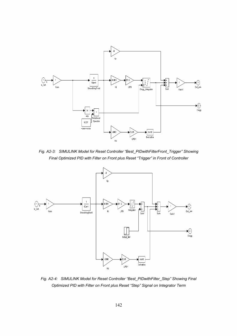
142
Fig. A2-3: SIMULINK Model for Reset Controller “Best_PIDwithFilterFront_Trigger” Showing
Final Optimized PID with Filter on Front plus Reset “Trigger” in Front of Controller
Fig. A2-4: SIMULINK Model for Reset Controller “Best_PIDwithFilter_Step” Showing Final
Optimized PID with Filter on Front plus Reset “Step” Signal on Integrator Term

143
Appendix 3:
Temperature-Cooling Control Loop Simulation Model (SIMULINK).
Fig. A3-1: Temperature-Cooling Control Loop SIMULINK Simulation Model (Selected Controllers)

144
Fig. A3-2: Temperature-Cooling Control Loop SIMULINK Simulation Model (All Controllers)