a dynamic model of sponsored search advertisingmela/bio/papers/yao_mela_2009.pdf · abstract: a...
TRANSCRIPT

A Dynamic Model of Sponsored Search Advertising
Song YaoCarl F. Mela1
May 1, 2009
1Song Yao (email: [email protected], phone: 919-660-2882) is a Ph.D. Candidate at Duke University,Durham, North Carolina, 27708. Carl F. Mela (email: [email protected], phone: 919-660-7767, fax: 919-681-6245) is a Professor of Marketing, The Fuqua School of Business, Duke University, Durham, North Carolina,27708. The authors would like to thank seminar participants at Cornell University, Dartmouth College, DukeUniversity, Emory University, Erasmus University, Georgia Institute of Technology, Georgia State University,Harvard Business School, INSEAD, London Business School, New York University, Northwestern Univer-sity, Ohio State University, Stanford University, University of British Columbia, University of California atBerkeley, University of Chicago, University of Maryland, University of Rochester, University of SouthernCalifornia, University of Texas, University of Tilburg, and the 2008 Marketing Science Conference as wellas J.P. Dubé, Wes Hartmann, Günter Hitsch, Han Hong, Anja Lambrecht, Andrés Musalem, Harikesh Nair,Peter Rossi and Rick Staelin for their feedback. We gratefully acknowledge �nancial support from the NETInstitute (www.netinst.org) and the Kau¤man Foundation.

Abstract: A Dynamic Model of Sponsored Search Advertising
Sponsored search advertising is ascendant� Jupiter Research reports expenditures rose 28% in 2007
to $8.9B and will continue to rise at a 26% CAGR, approaching 1/2 the level of television advertising
and making it one of the major advertising trends to a¤ect the marketing landscape. Yet little
empirical research exists to explore how the interaction of various agents (searchers, advertisers,
and the search engine) in keyword markets a¤ects consumer welfare and �rm pro�ts. The dynamic
structural model we propose serves as a foundation to explore these outcomes. We �t this model
to a proprietary data set provided by an anonymous search engine. These data include consumer
search and clicking behavior, advertiser bidding behavior, and search engine information such as
keyword pricing and website design.
With respect to the advertisers, we �nd evidence of dynamic bidding behavior. Advertiser value
for clicks on their sponsored links averages about 27 cents. Given the typical $22 retail price of the
software products advertised on the considered search engine, this implies a conversion rate (sales
per click) of about 1:2%, well within common estimates of 1-2% (gamedaily.com). With respect to
consumers, we �nd that frequent clickers place a greater emphasis on the position of the sponsored
advertising link. We further �nd that 10% of consumers do 90% of the clicks.
We then conduct several policy simulations to illustrate the e¤ects of changes in search engine
policy. First, we �nd the search engine obtains revenue gains of nearly 1:4% by sharing individual
level information with advertisers and enabling them to vary their bids by consumer segment. This
also improves advertiser revenue by 11% and consumer welfare by 2:9%: Second, we �nd that a
switch from a �rst to second price auction results in truth telling (advertiser bids rise to advertiser
valuations), consistent with economic theory. However, the second price auction has little impact on
search engine pro�ts. Third, consumer search tools lead to a platform revenue increase of 3:7% and
an increase of consumer welfare by 5:6%. However, these tools, by reducing advertising exposures,
lower advertiser pro�ts by 4:1%:
Keywords: Sponsored Search Advertising, Two-sided Market, Dynamic Game, Structural Models,Empirical IO, Customization, Auctions
1 Introduction
Sponsored search is one of the largest and fastest growing advertising channels. In January of 2009
alone, Internet users conducted 13:5B searches using the top 5 American search engines compared
to 10:5B in the previous January, indicating a robust 29% year over year increase.1 In the United
States, annual expenditures on sponsored search advertising increased 28% to $8:9B in 2007 and the
number of �rms using sponsored search advertising rose from 29% to 41%.2 Moreover, advertising
expenditures on sponsored search is forecast to grow to $25B by 2012.3 By contrast, overall 2007
television advertising spending in the United States is estimated to be $62B, an increase of only
0:7% from the preceding year.4 Hence, search engine marketing is becoming a central component
of the promotional mix in many organizations.
The growth of this new medium can be ascribed to several factors. First, the increasing popu-
larity of search engine sites relative to other media among consumers a¤ords a greater advertising
reach. In addition to searches on large general search engines such as Google.com, MSN.com, and
Yahoo.com, search is also widespread on more focused ones (dealtime.com searches Internet stores,
kayak.com searches travel products, addall.com searches books, etc.). The broad reach of search
can be ascribed to the complexity of wading through an estimated 155 million sites to return rel-
evant results in response to users�search queries.5 By comparison, a top rated TV show such as
�Desperate Housewives� only has about 25M viewers (IRI, 2007); and the growing popularity of
DVR services o¤ered by TiVo and cable companies have and will further decrease the audience
base of traditional TV advertising. Second, more and more consumers use the Internet for their
transactions (Ansari et al. (2008)), and Internet search is an especially e¢ cient way to promote
online channels. For example, Qiu et al. (2005) estimate that more than 13.6% of the web tra¢ c
is a¤ected by search engines. Third, search advertising often targets consumers who are actively
seeking information related to the advertisers� products. For example, a search of �sedan� and
�automotive dealer�might signal an active purchase state. As a result of these various factors,
Jupiter Research reports that 82% of advertisers were satis�ed or extremely satis�ed with search
marketing ROI in 2006 and 65% planned to increase search spending in 2007.6
Given the increasing ubiquity of sponsored search advertising, the topic has seen substantially
increased attention in marketing as of late (Ghose and Yang (2007), Rutz and Bucklin (2007), Rutz
and Bucklin (2008), Goldfarb and Tucker (2008)). These recent advances focus upon the e¢ cacy
1�January 2009 U.S. Search Engine Rankings,� comScore, Inc. (http://ir.comscore.com/releasedetail.cfm?ReleaseID=366442). �January 2008 U.S. Search Engine Rankings,� comScore, Inc. (http://www.comscore.com/press/release.asp?press=2068).
2�US Paid Search Forecast, 2007 to 2012,�Jupiter Research, 2007.3�US Interactive Marketing Forecast, 2007 to 2012,�Forrestor Research, 2007.4�Insider�s Report,�2007, McCann WorldGroup, Inc.; http://www.tns-mi.com/news/01082007.htm5�January 2008 Web Server Survey,� Netcraft Company (http://news.netcraft.com/archives/2008/01/28/
january_2008_web_server_survey.html).6�US Paid Search Forecast, 2007 to 2012,�Jupiter Research, 2007.
1

of an advertiser campaign. To date, empirical research on keyword search has been largely silent
on the perspective of the search engine, the competition between advertisers, and the behavior of
the searcher. Given that the search engine interacts with advertisers and searchers to determine
the price and consumer welfare of the advertising medium (and hence its e¢ cacy), our objective is
to broaden this stream of research to incorporate the role of all three agents: the search engine, the
advertisers, and the searchers. This exercise enables us to determine the role of search engine mar-
keting strategy on the behavior of advertisers and consumers as well as the attendant implications
for search engine revenues. Our key contributions are, accordingly, as follows:
1. From a theoretical perspective, we conceptualize and develop an integrated model of web
searcher, advertiser and search engine behavior. To our knowledge, this is the �rst empirical
paper focusing on the marketing strategy of the search engine. Much like Yao and Mela
(2008), we construct a model of a two-sided network in an auction context. One side of the
network includes the searchers who generate revenue for the advertiser. On the other side of
the two-sided network are advertisers whose bidding behavior determines the revenue of the
search engine. In the middle lies the search engine. The goal of the search engine is to price
consumer information, set auction mechanisms, and design webpages to elucidate product
information so as to maximize its pro�ts. Some key insights from this model include:
� Advertisers in our application have an average value per click of $0.27. Given that theaverage price of software products advertised on the site in our data is about $22, this
implies these advertisers expect about 1.2% (i.e., $0.27/$22) of clicks will lead to a pur-
chase. This is consistent with the industry average of 1-2% reported by GameDaily.com,
suggesting good face validity for our model.
� In addition, we �nd considerable heterogeneity in consumer response to sponsored searchadvertising. Frequent link clickers, who represent 10% of the population but 90% of the
clicks, tend to be more sensitive to slot order �in part because slot position can signal
product quality. These insights represent central inputs into our policy simulations
alluded to below.
2. From a substantive point of view, we o¤er concrete marketing policy recommendations to
the search engine. In particular, the two-sided network model of keyword search we consider
allows us to address the e¤ect of the following policy simulations (and would enable us to
address many others) on auction house and advertiser pro�ts as well as consumer welfare:
� Search Tools. Many search engines, especially specialized ones such as Shopping.com,provide users options to sort/�lter search results using certain criteria such as product
prices. On one hand, the search tools may mitigate the desirability of bidding for adver-
tisements because these tools can remove less relevant advertisements. This would tend
2

to lower search engine revenues. On the other hand, these tools can also attract more
users to the site leading to a potential increase in advertising exposures and searchers.
This would increase revenues. The trade-o¤ leads to the question of how search tools im-
pact consumer searching behavior, �rms�advertising decisions, and search engine pro�ts.
Our analysis indicates that negative consumer e¤ects on search engine pro�ts (�6:4%)outweigh the corresponding positive advertiser e¤ects on search engine pro�ts (2:7%) and
that overall the sort/�lter options enhance platform pro�ts by 3:7%. Consistent with
this result, there is a corresponding loss in consumer welfare of 5:6% and an attendant
increase in advertiser pro�ts of 4:1%.
� Segmentation and Targeting. Most search engines auction keywords across all marketsegments. However, it is possible to auction keywords by segment. This targeting
tends to reduce competition between advertisers within segments as markets are sliced
more narrowly, leading to lower bids and hence lower potential revenues for the search
engine. Yet targeting also enhances the e¢ ciency of advertising, which tends to increase
advertiser bids. Overall, we �nd that the latter e¤ect dominates (2:2%) the former
e¤ect (�0:8%) and that search engine revenue increases 1:4% by purveying keywords by
consumer market segments. Moreover, we �nd advertiser pro�ts improve by 11% (from
reduced competition in bidding and more e¢ cient advertising) and consumer welfare (as
measured by utility) increases 2:9%: Hence, this change leads to considerable welfare
gains across all agents.
� Market Intelligence. Advertisers�knowledge about consumers changes if search enginessell consumer demographic and behavioral information to advertisers. This raises the
question of whether and how information asymmetries between the engine and advertis-
ers a¤ect bidding behavior. We �nd that there is a negligible 0:08% increase in search
engine pro�ts accrued when this information asymmetry is erased. This �nding suggests
that advertisers are able to make reasonable inferences about the nature of heterogene-
ity in market response from the aggregate demand data, consistent with recent research
regarding individual level inference from aggregate demand (Chen and Yang (2007),
Musalem et al. (2008)). Moreover, the value of this information lies more in the adver-
tiser�s ability to exploit it by targeted bidding (as indicated in the preceding paragraph).
� Mechanism Design. The wide array of search pricing mechanisms raises the question
of which auction mechanism is the best in the sense of incenting advertisers to bid
more aggressively thereby yielding maximum returns for the search engine. We consider
two common mechanisms: a �rst price auction (as used by the considered �rm in our
analysis) and a second price auction (wherein a �rm pays the bid of the next lowest
bidder). Virtually no revenue gains accrue to the platform from a second price auction
(0:01%). However, advertiser bids under second price auction are close to bidders�true
3

values (bids average 98% of valuations), while bids under the �rst price auction are much
lower (72%). This �nding is consistent with theory that suggests �rst price auctions lead
to bid shading and second price auctions lead to truth telling (Edelman et al. (2007)).
Hence, we lend empirical validation to the theoretical literature on auction mechanisms
in keyword search.
3. From a methodological view, we develop a dynamic structural model of keyword advertising.
This dynamic is induced by the search engine�s use of past advertising performance when
ranking current advertising bids. The dynamic aspect of the problem requires the use of
some recent innovations pertaining to the estimation of dynamic games in economics (e.g.,
Bajari et al. (2007), Pesendorfer and Schmidt-Dengler (2008)). We extend this work to be
Bayesian in implementation and apply it to a wholly new context. Overall, we �nd that there
is a substantial improvement in model �t when the advertiser�s strategic bidding behavior is
considered (the log marginal likelihood improves by 50:0), consistent with the view that their
bidding behavior is dynamic. In addition, we �nd the posterior distributions of parameter
estimates is non-normal; while classical methods assume asymptotic normality, our Bayesian
approach does not.
Though we cast our model in the context of sponsored search, we note that the problem, and
hence the conceptualization, is even more general. Any interactive, addressable media format
(e.g., DVR, satellite digital radio) can be utilized to implement similar auctions for advertising.
For example, with the convergence in media between computers and television in DVRs, simple
channel or show queries can be accompanied by sponsored search, and this medium may help to
o¤set advertising losses arising from ads skipping by DVR users. In such a notion, the research
literature on sponsored search auctions generalizes to a much broader context, and our model serves
as a basis for exploring search based advertising.
The remainder of this paper proceeds as follows. First we overview the relevant literature to
di¤erentiate our analysis from previous research. Given the relatively novel research context, we
then describe the data to help make the problem more concrete. Next, we outline the details of
our model, beginning with the clicking behavior of consumers and concluding with the advertiser
bidding behavior. Subsequently, we turn to estimation and present our results. We then explore
the role of information asymmetry, targeted bidding, advertising pricing, and webpage design by
developing policy simulations that alter the search engine marketing strategies. We conclude with
some future directions.
4

2 Recent Literature
Research on sponsored search, commensurate with the topic it seeks to address, is nascent and
growing. Heretofore this literature can be characterized along two distinct dimensions: theoretical
and empirical. The theoretical literature details how agents (e.g., advertisers) are likely to react to
di¤erent pricing mechanisms. In contrast, the empirical literature measures the e¤ect of advertising
on consumer response in a given market but not the reaction of these agents to changes in the
platform environment (e.g., advertising pricing, information state or the webpage design of the
platform). By integrating the theoretical and empirical research streams, we develop a complete
representation of the role of pricing and information in the context of keyword search. To elaborate
on these points, we begin by surveying theoretical work on sponsored search and then proceed to
discuss some recent empirical research.
Foundational theoretical analyses of sponsored search include Edelman et al. (2007) and Varian
(2007) who examine the bidding behaviors of advertisers in this auction game. The authors assume
the auction game as a complete information and simultaneous-move static game, in which exoge-
nous advertising click-through rates increase with better placements. In equilibrium advertiser
bidding behavior has the same payo¤ structure as a Vickrey-Clarke-Groves auction, where a win-
ner�s payment to the seller equals to those losing bidders�potential payo¤s (opportunity costs) were
the winner absent (Groves (1979)). Extending this work, Chen and He (2006) incorporate clicking
behavior into their model and show that, under the Google bidding mechanism, consumers clicking
behavior is a¤ected by access to product information. In particular, they make inferences about
product quality based on the ranking presented by the platform and search sequentially according
to the ranking. As an equilibrium response, advertisers submit bids equal to their true values for
the advertising. Athey and Ellison (2008) also consider a model that integrates both consumers
and advertisers as in Chen and He (2006) but make several important extensions. They assume
that advertisers only know the distribution of their competitors�valuations about sponsored slots,
thus making the auction an incomplete information game. They also assume consumers engage in
costly sequential searches that follow an optimal stopping rule (cf. Weitzman (1979)): consumers
stop searching when the expected return of further searching is lower than the best choice in their
consideration set. Thus, the better slot an advertiser gets, the higher the probability that her
product will be purchased by consumers. Intuitively, this is because a better spot will give the
product a higher probability to be included in the consumer�s consideration set before she stops
searching. So a better slot implies higher sales for the advertiser. The equilibrium bidding strat-
egy in Athey and Ellison (2008) is di¤erent than those in previous literature. Although bids are
still monotonically increasing in values (qualities), high value (quality) advertisers will bid more
aggressively than low value (quality) advertisers. Katona and Sarvary (2008) further extend the
analysis by relaxing several key assumptions such as the competition for tra¢ c between sponsored
5
links and organic links, the heterogeneity of advertisers in term of their inherent attractiveness to
consumers. The author shows multiple equilibria in this auction which do not have closed form
solutions. Additional work by Iyengar and Kumar (2006), Feng (2008), and Garg et al. (2006)
explicitly consider the e¤ect of the various auction mechanisms on search engine pro�ts. In partic-
ular, Iyengar and Kumar (2006) show that the Google pricing mechanism maximizes neither the
search engine�s revenue nor the e¢ ciency of the auction suggesting the potential to improve on this
mechanism as we seek to do. Further, they show that the optimal mechanism is incumbent upon
the characteristics of the market, thereby making it imperative to estimate market response as we
intend to do in order to improve on pricing mechanisms. Summarizing the key insights from this
stream of work, we note that i) there are three agents interacting in the sponsored search context,
those who engage in keyword search, advertisers that bid for keywords, and the search platform,
ii) searchers a¤ect advertisers bidding behavior by reacting to the search engine�s web page design
and hence advertiser payo¤s, iii) bidders a¤ect searcher behavior by the placement of their adver-
tisements on the page, and iv) changes in advertiser and consumer behavior are incumbent upon
the strategies of the platform.
In spite of these insights, several limits remain. First, because equilibrium outcomes are incum-
bent upon the parameters of the system, it is hard to characterize precisely how agents will behave.
This implies it would be desirable to estimate a model of keyword search in order to measure these
behaviors. Second, a static advertiser game over bidding periods is typically assumed, which is
inconsistent with the pricing practices used by search engines. Search engines commonly use the
preceding period�s click-throughs together with current bids to determine advertising placement,
making this an inherently dynamic game. Third, this research typically assumes no asymmetry
in information states between the advertiser and the search engine even though the search engine
knows individual level clicking behaviors and the advertiser does not. We redress these issues in
this paper.
Empirical research on sponsored search advertising is also proliferating. Notable among these
papers, Rutz and Bucklin (2008) investigate the e¢ cacy of di¤erent keyword choices by measuring
the conversion rate from users� clicks on ads to actual sales for the advertiser. In a related pa-
per, Rutz and Bucklin (2007) considers how advertiser revenue is a¤ected by click-throughs and
exposures. This work is important because it demonstrates that advertiser valuations di¤er for
various placements and keywords, and that the bids are likely to be related to placements. Ghose
and Yang (2007) further investigate the relationships among di¤erent metrics such as click-through
rate, conversion rate, bid price, and advertisement rank. Though extant empirical research on
sponsored search establishes a �rm link between advertising, slot position, and revenues �and indi-
cates that these e¤ects can di¤er across advertisers, some limitations of this stream of work remain.
First, it emphasizes a single agent (one advertiser), making it di¢ cult to predict how advertisers
in an oligopolistic setting might react to a change in the auction mechanism, webpage design, or
6
information state regarding consumers. Competitive interactions are material to understanding the
role of each agent in the context of sponsored search. For example, an advertiser�s value to the
search engine pertains not only to its direct payment to the search engine but also to the indirect
e¤ect that advertiser has on the intensity of competition during bidding. The increased intensity
of competition may serve to drive bids upward and hence increase search engine revenues. Second,
the advertisers�actions a¤ect search engine users and vice-versa. For example, with alternative
advertisers being placed at premium slots on a search result page, it is likely that users�browsing
behaviors will be di¤erent. As advertisers make decisions with the consideration of users�reactions,
any variations of users�behaviors provide feedback on advertisers�actions and thus will ultimately
a¤ect the search engine revenue.
Integrating these two research streams suggests it is desirable to both model and estimate the
equilibrium behavior of all the agents in a network setting. In this regard, sponsored search adver-
tising can be characterized as a two-sided market wherein searchers and advertisers interact on the
platform of the search engine (Rochet and Tirole (2006)). This enables us to generalize a structural
modeling approach advanced by Yao and Mela (2008) to study two-sided markets. These authors
model bidder and seller behavior in the context of electronic auctions to explore the e¤ect of auc-
tion house pricing on the equilibrium number of listings and closing prices. However, additional
complexities exist in the keyword search setting including: i) the aforementioned information asym-
metry between advertisers and the search engine and ii) the substantially more complex auction
pricing mechanism used by search engines relative to the �xed fee auction house pricing considered
in Yao and Mela (2008). Moreover, unlike the pricing problem addressed in Yao and Mela (2008),
sponsored search bidding is inherently dynamic owing to the use of lagged advertising click rates
to determine current period advertising placements. Hence we incorporate the growing literature
of two-step dynamic game estimation (e.g., Hotz and Miller (1993); Bajari et al. (2007); Bajari
et al. (2008)). Instead of explicitly solving for the equilibrium dynamic bidding strategies, the
two-step estimation approach assumes that observed bids are generated by equilibrium play and
then use the distribution of bids to infer underlying primitive variables of bidders (e.g., the adver-
tiser�s expectation about the return from advertising). A similar method is also used in an auction
context in Jofre-Bonet and Pesendorfer (2003). However, our approach is unique inasmuch as it is
a Bayesian instantiation of these estimators, which leads to desirable small sample properties and
enables considerable �exibility in modeling choices. Equipped with these advertiser primitives, we
solve the dynamic game played by the advertiser to ascertain how changes in search engine policy
a¤ect equilibrium bidding behavior.
7

3 Empirical Context
The data underpinning our analysis is drawn from a major search engine for high technology
consumer products. Within this broad search domain, we consider search for music management
software because the category is relatively isolated in the sense that searches for this product do
not compete with others on the site.7 The category is a sizable one for this search engine as well.
Along with the increasing popularity of MP3 players, the use of music management PC software is
increasing exponentially, making this an important source of revenue. The goal of the search engine
is to enable consumers to identify and then download trial versions of these software products before
their �nal purchase.8 It is important to note that the approach we develop can readily generalize
to other contexts and that we consider this particular instantiation to be a particular illustration
of a more general approach.
3.1 Data Description
The data are comprised of three �les, including:
� Bidding �le. Bidding is logged into a �le containing the bidding history of all active biddersfrom January 2005 to August 2007. It records the exact bids submitted, the time of each
bid submission, and the resulting monthly allocation of slots. Hence, the unit of analysis is
vendor-bid event. These data form the cornerstone of our bidding model.
� Product �le. Product attributes are kept in a �le that records, for each software �rm in each
month, the characteristics of the software they purvey. This �le also indicates the download
history of each product in each month.
� Consumer �le. Consumer log �les record each visit to the site and are used to infer whetherdownloads occur as well as browsing histories. A separate but related �le includes registration
information and detailed demographics for those site visitors that are registered. These data
are central to the bidding model in the context of complete information.
We detail each of these �les in turn.7The search engine de�nes music management broadly enough that an array of di¤erent search terms (e.g., MP3,
iTunes, iPod, lyric, etc.) yield the same search results for the software products in this category. Hence we considerthe consumer decision of whether to search for music software on the site and whether to download given a search.
8A �click�and a �download�are essentially the same from the perspectives of the advertiser, consumer, and searchengine. In the �click�case, a consumer makes several clicks to investigate and compare products o¤ered by di¤erentvendors and then makes a �nal purchase. In the �download�case, a consumer downloads several products and makesthe comparison before �nal purchase. Hence there is no di¤erence for a �click� and a �download� in the currentcontext. We use �click�and �download� interchangeably throughout the paper.
8
3.1.1 Bidding File
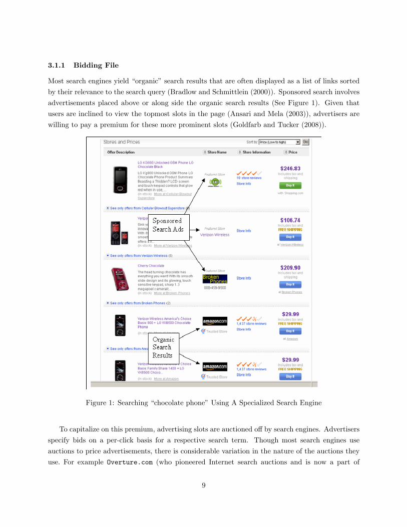
Most search engines yield �organic�search results that are often displayed as a list of links sorted
by their relevance to the search query (Bradlow and Schmittlein (2000)). Sponsored search involves
advertisements placed above or along side the organic search results (See Figure 1). Given that
users are inclined to view the topmost slots in the page (Ansari and Mela (2003)), advertisers are
willing to pay a premium for these more prominent slots (Goldfarb and Tucker (2008)).
Figure 1: Searching �chocolate phone�Using A Specialized Search Engine
To capitalize on this premium, advertising slots are auctioned o¤ by search engines. Advertisers
specify bids on a per-click basis for a respective search term. Though most search engines use
auctions to price advertisements, there is considerable variation in the nature of the auctions they
use. For example Overture.com (who pioneered Internet search auctions and is now a part of
9

Yahoo!) adopted a �rst price auction wherein the advertiser bidding the highest amount per click
received the most prominent placement at the cost of its own bid for each click.9 First price auctions
are still used by Shopping.com and a number of other Internet properties. Google has developed
an algorithm which factors in not only the level of the bid, but the expected click-through rate of
the advertiser. This enhances search engine revenue because these revenues depend not only on
the per-click bid, but also the number of clicks a link receives. Another distinction of the Google
practice is that advertisers pay the next bidder�s bid (adjusted for click-through rates) as opposed
to their own bids.10
The mechanism used by the �rm we consider is similar to that of Google except that the
considered search engine uses a �rst price auction in place of a second price auction (we intend to
compare the e¢ cacy of this mechanism to that of Google in our policy experiments). Winning
bids are denoted as sponsored search results and the site �ags these as sponsored links. The site we
consider a¤ords up to �ve premium slots which is far less than the 400 or so products that would
appear at the search engine. Losing bidders and non-bidders are listed beneath the top slots on
the page and like previous literature we denote these listings as organic search results.
These advertiser bidding histories by month are all captured in a database. In particular,
the search engine collects bidding and demographic data on all advertisers (products attributes,
products download history, and bids from active bidders). We detail these data next. Table 1
reports summary statistics for the bidding �les. At this search engine, bids were submitted on a
monthly basis. Over the 32 months from January 2005 to August 2007, 322 bids (including zeros)
were submitted by 21 software companies.11 As indicated in Table 1, bidders on average submitted
about 22 positive bids in this interval (slightly less than once per month). The average bid amount
(conditioned on bidding) was $0.20 with a large variance across bidders and time.
Table 1: Bids Summary Statistics
Mean Std. Dev. Minimum MaximumNon-zero Bids (c/) 19.55 8.32 15 55Non-zero Bids/Bidder 21.78 10.46 1 30All Bids (c/) 8.14 11.04 0 55Bids/Bidder 23.13 9.68 1 32
9 In the economics literature, such an auction with multiple items (slots) where bidders pay what they bid issometimes termed as discriminatory auction (Krishna (2002)).10With a simpli�ed setting, Edelman et al. (2007) show that the Google practice may result in an equilibrium
with bidders�payo¤s equivalent to the Vickrey-Clarke-Groves (VCG) auction, whereas VCG auction has been provedto maximize total payo¤s to bidders (Groves (1979)). Iyengar and Kumar (2006) further show that under someconditions the Google practice induces VCG auction�s dominant �truth-telling� bidding strategy, i.e., bidders willbid their own valuations.11Since some products were launched after January 2005, they were not observed in all periods.
10

3.1.2 Product File
Searching for a keyword on this considered site results in a list of relevant software products and
their respective attributes. Attribute information is stored in a product �le along with the download
history of all products that appeared in this category from January 2005 to August 2007. In total,
these data cover 394 products over 32 months. The attributes include the price of the non-trial
version of a product, backward compatibility with preceding operating systems (e.g., Windows
98 and Windows Server 2003), expert ratings provided by the site, and consumer ratings of the
product.12 Trial versions typically come with a 30-day license to use the product for free, after
which consumers are expected to pay for its use. Expert ratings at the site are collected from
several industrial experts of these products. The consumer rating is based on the average feedback
score about the product from consumers. Tables 2 and 3 give summary statistics for all products
as well as active bidders�products. Based on the compatibility information, we sum each product�s
compatibility dummies and de�ne this summation as a measure for that product�s compatibility
with older operating systems. This variable is later used in our estimation.
Table 2: Product Compatibility
PercentageAll ProductsWindows NT 4.0 54Windows 98 64Windows Me 66Windows 2000 91Windows Server 2003 43
Bidders�ProductsWindows NT 4.0 67Windows 98 67Windows Me 71Windows 2000 85Windows Server 2003 57
Overall, active bidders�products have higher prices, better ratings, and more frequent updates.
3.1.3 Consumer File
The consumer �le contains the log �les of consumers from May 2007 to August 2007. This �le
contains each consumer�s browsing log when they visit the search engine both within the search site
and across Internet properties owned by the search site. The consumer �le also has the registration
information for those that register.
12We further considered �le size but found many missing values. Moreover, in light of increased Internet speed, �lesize has become somewhat inconsequential in the download decision and thus is omitted from our analysis.
11
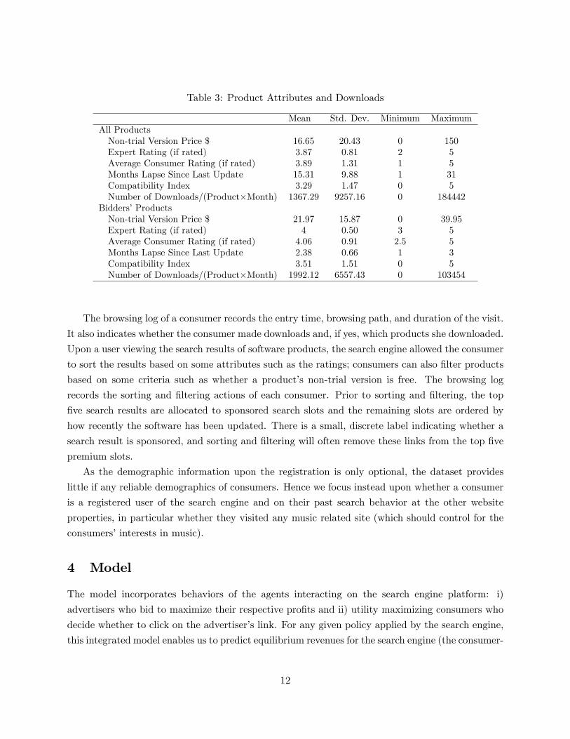
Table 3: Product Attributes and Downloads
Mean Std. Dev. Minimum MaximumAll ProductsNon-trial Version Price $ 16.65 20.43 0 150Expert Rating (if rated) 3.87 0.81 2 5Average Consumer Rating (if rated) 3.89 1.31 1 5Months Lapse Since Last Update 15.31 9.88 1 31Compatibility Index 3.29 1.47 0 5Number of Downloads/(Product�Month) 1367.29 9257.16 0 184442
Bidders�ProductsNon-trial Version Price $ 21.97 15.87 0 39.95Expert Rating (if rated) 4 0.50 3 5Average Consumer Rating (if rated) 4.06 0.91 2.5 5Months Lapse Since Last Update 2.38 0.66 1 3Compatibility Index 3.51 1.51 0 5Number of Downloads/(Product�Month) 1992.12 6557.43 0 103454
The browsing log of a consumer records the entry time, browsing path, and duration of the visit.
It also indicates whether the consumer made downloads and, if yes, which products she downloaded.
Upon a user viewing the search results of software products, the search engine allowed the consumer
to sort the results based on some attributes such as the ratings; consumers can also �lter products
based on some criteria such as whether a product�s non-trial version is free. The browsing log
records the sorting and �ltering actions of each consumer. Prior to sorting and �ltering, the top
�ve search results are allocated to sponsored search slots and the remaining slots are ordered by
how recently the software has been updated. There is a small, discrete label indicating whether a
search result is sponsored, and sorting and �ltering will often remove these links from the top �ve
premium slots.
As the demographic information upon the registration is only optional, the dataset provides
little if any reliable demographics of consumers. Hence we focus instead upon whether a consumer
is a registered user of the search engine and on their past search behavior at the other website
properties, in particular whether they visited any music related site (which should control for the
consumers�interests in music).
4 Model
The model incorporates behaviors of the agents interacting on the search engine platform: i)
advertisers who bid to maximize their respective pro�ts and ii) utility maximizing consumers who
decide whether to click on the advertiser�s link. For any given policy applied by the search engine,
this integrated model enables us to predict equilibrium revenues for the search engine (the consumer-
12

Figure 2: Consumer Decisions
advertiser interactions are analogous to a sub-game contingent on search engine behavior). The
behavior of the bidder (advertiser) is dependent on the behavior of the consumer as consumer
behavior a¤ects advertiser expectations for downloads and, hence, their bids. The behavior of
the consumer is dependent upon the advertiser because the rank of the advertisement a¤ects the
behavior of the consumer. Hence, the behaviors are interdependent. Because advertisers move
prior to consumers�actions in this game, we �rst exposit the consumer model and then solve the
bidder problem in a backward deduction manner.
4.1 Consumer Model
Advertiser pro�t (and therefore bidding strategy) is incumbent upon their forecast of consumer
downloads for their products dtj(k;Xtj ; c), where k denotes the position of the advertisement on
the search engine results page, Xtj indicate the attributes of the advertiser j�s product at time t,
and c are parameters to be estimated. Thus, we seek to develop a forecast for dtj(k;Xtj ; c) and
the attendant consequences for bidding. To be consistent with the advertisers information set, we
begin by basing these forecasts of consumer behavior solely on statistics observed by the advertiser:
the aggregate download data and the distribution of consumers characteristics. Later, in the policy
section of the paper, we assess what happens to bidding behavior and platform revenues when
disaggregate information is revealed to advertisers by the platform. We begin by describing the
consumer�s download decision process and how it a¤ects the overall number of downloads.
4.1.1 The Consumer Decision Process
Figure 2 overviews the decisions made by consumers. In any given period t, the consumer�s problem
is whether and which software to select in order to maximize their utility. The resolution of this
problem is addressed by a series of conditional decisions.
13
First, the consumer decides whether she should search on the category considered in this analysis
(C1). We presume that the consumer will search on the site if it maximizes her expected utility.13
Conditioned upon engaging a search, the consumer next decides whether to sort and/or �lter
the results (C2). The two search options lead to the following 4 options for viewing the results:
� ={0 � neither, 1 � sorting but not �ltering, 2 � not sorting but �ltering, 3 � sorting and
�ltering}. For each option, the set of products returned by the search engine di¤ers in terms of the
number and the order of products. Consumers choose the sorting/�ltering option that maximizes
their expected utility.
Third, the consumer then chooses which, if any products to download (C3). We presume that
consumers choose to download software if it maximizes their expected utility. We discuss the
modeling details for this process in a backward induction manner (C3�C1).
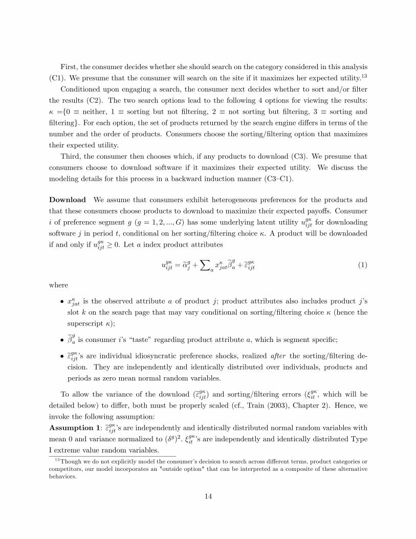
Download We assume that consumers exhibit heterogeneous preferences for the products and
that these consumers choose products to download to maximize their expected payo¤s. Consumer
i of preference segment g (g = 1; 2; :::; G) has some underlying latent utility ug�ijt for downloading
software j in period t, conditional on her sorting/�ltering choice �. A product will be downloaded
if and only if ug�ijt � 0. Let a index product attributes
ug�ijt = e�gj +Xax�jat
e�ga + e"g�ijt (1)
where
� x�jat is the observed attribute a of product j; product attributes also includes product j�sslot k on the search page that may vary conditional on sorting/�ltering choice � (hence the
superscript �);
� e�ga is consumer i�s �taste�regarding product attribute a, which is segment speci�c;� e"g�ijt�s are individual idiosyncratic preference shocks, realized after the sorting/�ltering de-cision. They are independently and identically distributed over individuals, products and
periods as zero mean normal random variables.
To allow the variance of the download (e"g�ijt) and sorting/�ltering errors (�g�it , which will bedetailed below) to di¤er, both must be properly scaled (cf., Train (2003), Chapter 2). Hence, we
invoke the following assumption:
Assumption 1: e"g�ijt�s are independently and identically distributed normal random variables with
mean 0 and variance normalized to (�g)2. �g�it �s are independently and identically distributed Type
I extreme value random variables.13Though we do not explicitly model the consumer�s decision to search across di¤erent terms, product categories or
competitors, our model incorporates an "outside option" that can be interpreted as a composite of these alternativebehaviors.
14

Under assumption 1, we may re-de�ne the utility in Equation 1 as
ug�ijt = �g(�gj +X
ax�jat�
ga| {z }
ug�ijt
+ "g�ijt) (2)
where f�gj ; �ga; "g�ijtg = fe�gj ; e�ga;e"g�ijtg=�g; ug�ijt is the scaled �mean�utility and "g�ijt � N(0; 1). The
resulting choice process is a multivariate probit choice model.14 Let dijt = 1 stand for downloading
and dijt = 0 stand for not downloading. We have
dijt =
(1
0
if ug�ijt � 0otherwise
(3)
and the probability of downloading conditional on parameters f�gj ; �gag is
Pr(dijt = 1) = Pr(ug�ijt � 0) (4)
= Pr(�g(ug�ijt + "g�ijt) � 0)
= Pr(�"g�ijt � ug�ijt)
= �(ug�ijt)
where �(�) is the standard normal distribution CDF.
Sorting and Filtering Prior to making a download decision, consumers face several �ltering
and sorting options which we index as � = 0; 1; 2; 3. We expect consumers to choose the option
that maximizes their expected download utility. Although consumers know the distribution of
the product utility error terms (e"g�ijt), these error terms do not realize before the sorting/�ltering.Hence consumers can only form an expectation about the total utilities of all products under a
given sorting/�ltering option � before choosing that option. Let Ug�it denote the total expected
utility from products under option �, which can be calculated based on Equation 1:
Ug�it =Xj
E"(ug�ijtju
g�ijt � 0)Pr(u
g�ijt � 0): (5)
This de�nition re�ects that a product�s utility is realized only when it is downloaded. Hence,
the expected utility E"(ug�ijtju
g�ijt � 0) is weighted by the download likelihood, Pr(ug�ijt � 0). The
expectation, E"(�), is taken over the random preference shocks "g�ijt.
In addition to Ug�it , individuals may accrue additional bene�ts or costs for using sorting/�ltering
option �. These bene�ts or costs may arise from individual di¤erences of e¢ ciency or experience
14 It can be shown that, under very weak assumptions, download decisions across multiple products with the purposeof maximizing total expected utility can be represented by a multivariate binary choice probit model.
15

in terms of engaging the various options for ordering products. We denote such bene�ts or costs
by random terms �g�it �s. As indicated in assumption 1, �g�it �s are i.i.d. Type I extreme value. �
g�it is
not observed by researchers but known to individual i. Note that these sorting/�ltering bene�ts or
costs do not materialize during the consumption of the products. Therefore, they do not enter the
latent utility in Equation (1). The total utility of search option � is thus given by
zg�it = Ug�it + �g�it : (6)
Consumers choose the option of sorting/�ltering that leads to the highest total utility zg�it .
With �g�it following a Type I extreme value distribution, the choice of sorting/�ltering becomes
a logit model such that
Pr(�)git =exp(Ug�it )3P
�0=0exp(Ug�
0
it )
(7)
To better appreciate the properties of this model, note that Ug�it in Equation 5 can be written
in a closed form:15
Ug�it =Xj
E"(ug�ijtju
g�ijt � 0) � Pr(u
g�ijt � 0) (8)
= �gXj
ug�ijt +
�(ug�ijt)
�(ug�ijt)
!� �(ug�ijt):
With such a formulation, the factors driving the person�s choice of �ltering or sorting become
more apparent:
� Filtering eliminates options with negative utility, such as highly priced products (becauseconsumer price sensitivity is negative). As a result, the summation in Equation 8 for the
�lter option will increase as the negative ug�ijt are removed. This raises the value of the �lter
option suggesting that price sensitive people are more likely to �lter on price.
15For a normal random variable x with mean �, standard deviation � and left truncated at a (Greene (2003)),
E(xjx � a) = �+ ��(a���), where �(a��
�) is the hazard function such that �(a��
�) =
�( a���
)
1��( a���
).
Hence with ug�ijt � N(�gug�ijt; (�
g)2), we have
E(ug�ijtjug�ijt � 0)
= (�g � ug�ijt + �g �
�(� �g�ug�ijt�g
)
1� �(� �g�ug�ijt�g
))
= �g(ug�ij +�(ug�ij )
�(ug�ij ))
16

� Sorting re-orders products by their attribute levels. Products that appear low on a page willtypically have lower utility regardless of their product content (because consumer slot rank
sensitivity is negative). For example, suppose a consumer relies more on product ratings. By
moving more desirable items that have high ratings up the list, sorting can increase the ug�ijtfor these items, thereby increasing the resulting summation in Equation 8 and the value of
this sorting option.16
Keyword Search The conditional probability of keyword search takes the form
Pr(searchgi ) =exp(�g0 + �
g1IV
git )
1 + exp(�g0 + �g1IV
git )
(9)
where IV gi is the inclusive value for searching conditional on the segment membership. IV g
it is
de�ned as
IV git = log[
X�exp(Ug�it )]: (10)
This speci�cation can be interpreted as the consumer making a decision to use a keyword search
based on the rational behavior of utility maximization (McFadden (1977); Ben-Akiva and Lerman
(1985)).17 A search term is more likely to be invoked if it yields higher expected utility.
Segment Membership Recognizing that consumers are heterogeneous in behaviors described
above, we apply a latent class model in the spirit of Kamakura and Russell (1989) to capture
heterogeneity in consumer preferences. Heterogeneity in preference can arise, for example, when
some consumers prefer some features more than others. We assume G exogenously determined
segments.18 Note that our speci�cation implies a dependency across decisions within the same
segment that is not captured via the stage-speci�c decision errors, and therefore captures the e¤ect
of unobserved individual speci�c di¤erences in search behavior.
The prior probability for user i being a member of segment g is de�ned as
pggit = exp� g0 +Demo
0it
g�=�Gg0=1 exp
� g
0
0 +Demo0it
g0�
(11)
where Demo0it is a vector of attributes of user i such as demographics and past browsing his-
tory; vector f g0; gg8g contains parameters to be estimated. For the purpose of identi�cation, onesegment�s parameters are normalized to zero.
16 In particular, in the data over 80% of consumers who used the sorting option chose ratings to re-order products.Thus, we suspect that consumers who rely on ratings are more likely to use the sorting option to see which items arethe most popular ones.17This speci�cation is consistent with the consumer information structure such that �g�i is not observed by re-
searchers but known to consumer i.18 It is possible to allow for continous mixtures of heterogeneity as well. In our application, many consumers enter
only once, making it di¢ cult to identify a consumer speci�c term for them.
17

4.1.2 Consumer Downloads
The search, sort/�lter, and download models can be integrated to obtain an expectation of the
number of downloads that an advertiser receives for a given position of its keyword advertisement.
Advertisers must form this expectation predicated on observed aggregate download totals, dtj (in
contrast to the search engine who observes yijt; �it and Demoit).19
To develop this aggregate download expectation, we begin by noting that the download utility
ug�ijt is a function of consumer speci�c characteristics and decisions �ijt = ["g�ijt; �
g�it ; search
gi , segment
g membership, Demo0it] and that an advertiser needs to develop an expectation of downloads over
the distribution of these unobserved (to the advertiser) individual characteristics. De�ne
Aijt = f�ijt : ug�ijt � 0g;
i.e., Aijt is the set of values of �ijt which will lead to the download of product j in period t.
Let D(�ijt) denote the distribution of �ijt. The likelihood of downloading product j in period tcan be expressed as
P tj =
Z�ijt2Aijt
D(�ijt) (12)
=
ZDemoit
Xg
X�[�(ug�ijt)
exp(Ug�it )3P
�0=0exp(Ug�
0
it )
] Pr(searchgit)pggitdD(Demoit) (13)
where the �rst term in the brackets captures the download likelihood, the second term captures the
search strategy likelihood, and the �rst term outside the brackets captures the likelihood of search.
pggit is the probability of segment g membership and D(Demoit) is the distribution of demographics.Correspondingly, the advertiser with attributes Xt
j has an expected number of downloads for
appearing in slot k, dtj(k;Xtj ; c), which can be computed as follows
dtj(k;Xtj ; c) =MtP
tj (14)
where c is the set of consumer preference parameters; Mt is the market size in period t; and Xtj
is the vector of the a product characteristics, xjat.
Product attributes are posted on the search engine and are therefore common knowledge to all
advertisers and consumers. We assume these Xtj are exogenous within the scope of our sponsored
search analysis for several reasons. First, advertisers distribute and promote their products through
multiple channels and they do so over longer periods of time than considered herein. Hence, product
19We discuss the corresponding advertiser download expectation under complete information in section 7.3.
18

Figure 3: Advertiser Decisions
attributes are more likely to be determined via broader strategic considerations than the particular
auction game and time frame we consider. Second, the attribute levels for each product are stable
over the duration of our data and analysis. We would expect more variation in attribute levels if
they were endogenous to the particular advertiser and search engine decisions we consider. Third,
because there is little or no variation in product attributes over time, it is not feasible to estimate
endogenous attribute decision making with our data.
4.2 Advertiser Model
Figure 3 overviews the dynamic game played by the advertiser. Advertiser j�s problem is to
decide the optimal bid amount btj with the objective of maximizing discounted present value of
payo¤s.20 Higher bids lead to greater revenues because they yield more favorable positions on the
search engine, thereby yielding more click-throughs for the advertiser. However, higher bids also
increase costs (payments) leading to a trade-o¤ between costs and revenues. The optimal decision
of whether and how much to bid is incumbent upon the bidding mechanism, the characteristics of
the advertiser, the information available at the time of bidding (including the state variables), and
the nature of competitive interactions.
An advertiser�s period pro�t for a download is the value it receives from the download less
the costs (payments) of the download. Though we do not observe the value of a download, we
20Because the search engine used in our application has the dominant market share in the considered category, wedo not address advertiser bidding on other sites. Also, it would be di¢ cult to obtain download data from these moreminor competitors. We note this is an important issue and call for future research.
19

infer this value by noting the observed bid can be rationalized only for a particular value accrued
by the advertiser. We presume this value is drawn from a distribution known to all �rms. The
total period revenue for the advertiser is then the value per download times the expected number
of downloads.21 The total period payment upon winning is the number of downloads times the
advertiser�s bid. Hence, the total expected period pro�t is the number of downloads times the pro�t
per download (i.e., the value per downloads less the payment per download).
Of course, the bid levels and expected download rates are a¤ected by rules of the auction.
Though we elaborate in further details on the speci�c rules of bidding below, at this point we simply
note that the rules of the auction favor advertisers whose products were downloaded more frequently
in the past since such products are more likely to lead to higher revenues for the platform.22 Current
period downloads are, in turn, a¤ected by the position of the advertisement on the search engine.
Because past downloads a¤ect current placement, and thus current downloads, the advertiser�s
problem is inherently dynamic; and past downloads are treated as a state variable.
Finally, given the rules of the auction, we note that all advertisers move simultaneously. While
we presume a �rm knows its own value, we assume competing �rms know only the distribution of
this value.
The process is depicted in Figure 3. We describe the process with more details as follows:
Section 4.2.1 details the rules of the auction that a¤ect the seller costs (A2), section 4.2.2 details
the advertisers�value distribution (A1), and section 4.2.3 indicates how period values and costs
translate to discounted pro�ts and the resulting optimal bidding strategy (A3).
4.2.1 Seller Costs and the Bidding Mechanism
We begin by discussing how slot positions are allocated with respect to bids and the e¤ect of these
slot positions on consumer downloads (and thus advertiser revenue).
Upon a consumer completing a query, the search engine returns k = 1; 2; :::K; :::; N slots covering
the products of all �rms. Only the top K = 5 slots are considered as premium slots. Auctions for
these K premium slots are held every period (t = 1; 2; :::). An advertiser seeks to appear in a more
prominent slot because this may increase demand for the advertiser�s product. Slots K + 1 to N
are non-premium slots which compose a section called organic search section.
There are N advertisers who are interested in the premium slots (N � N). In order to procure
a more favorable placement, advertiser j submits bid btj in period t. These bids, submitted simul-
taneously, are summarized by the vector bt = fbt1; bt2; :::; btNg.23 Should an advertiser win slot k,21The expected number of downloads is inferred form the consumer model and we have derived this expression in
section 4.1.2.22This is because the payment made to the search engine by an advertiser is the advertiser�s bid times its total
downloads.23For the purpose of a clear exposition, we sometimes use boldface notations or pairs of braces to indicate vectors
whose elements are variables across all bidders. For example, dt = fdtjg8j is a vector whose elements are dtj ;8j.
20

the realized number of downloads dtj is a random draw from the distribution with the expectation
dtj(k;Xtj ; c). The placement of advertisers into the K premium slots is determined by the ranking
of their fbtjdt�1j g8j , i.e., the product of current bid and last period realized downloads; the topmostbidder gets the best premium slot; the second bidder gets the second best premium slot; and so on.
A winner of one premium slot pays its own bid btj for each download in the current period. Hence,
the total payment for winning the auction is btjdtj .
If an advertiser is not placed at one of the K premium slots, it will appear in the organic section;
advertisers placed in the organic section do not pay for downloads from consumers. The ranking
in the organic search section is determined by the product update recency at period t, which is a
component of the attribute vector of each product, Xtj . Other attributes include price, consumer
ratings, and so on.
Given that the winners are determined in part by the previous period�s downloads, the auction
game is inherently dynamic. Before submitting a bid, the commonly observed state variables at
time t are the realized past downloads of all bidders from period t� 1,24
st = dt�1 = fdt�11 ; dt�12 ; :::; dt�1N g: (15)
4.2.2 Seller Value
The advertiser�s bid determines the cost of advertising and must be weighed against the potential
return when deciding how much to bid. We denote advertiser j�s valuation regarding one download
of its product in period t as vtj . We assume that this valuation is private information but drawn
from a normal distribution that is commonly known to all advertisers. Speci�cally,
vtj = v(Xtj ; �) + fj + r
tj (16)
= Xtj� + fj + r
tj
where � are parameters to be estimated and re�ect the e¤ect of product attributes on valuation. The
fj are �rm-speci�c �xed e¤ect terms assumed to be identically and independently distributed across
advertisers. This �xed e¤ect term captures heterogeneity in valuations that may arise from omitted
�rm-speci�c e¤ects such as more e¢ cient operations. The rtj � N(0; 2) are private shocks to an
advertiser�s valuation in period t, assumed to be identically and independently distributed across
advertisers and periods. The sources of this private shock may include: (1) temporary increases in
the advertiser�s valuation due to some events such as a promotion campaign; (2) unexpected shocks
to the advertiser�s budget for �nancing the payments of the auction; (3) temporary production
capacity constraint for delivering the product to users; and so on. The random shock rtj is realized
24Though state variables can be categorized as endogeneous (past downloads) and exogenous (product attributes),our exposition characterizes only downloads as state variables because these are the only states whose evolution issubject to a dynamic constraint.
21

at the beginning of period t. Although rtj is private knowledge, we assume the distribution of
rtj � N(0; 2) is common knowledge among bidders. We further assume the �xed e¤ect fj of
bidder j is known to all bidders but not to researchers. Given bidders may observe opponents�
actions for many periods, the �xed e¤ect can be inferred among bidders (Greene (2003)).
4.2.3 Seller Pro�ts: A Markov Perfect Equilibrium (MPE)
Given vtj and state variable st, predicted downloads and search engine�s auction rules, bidder j
decides the optimal bid amount btj with the objective of maximizing discounted present value of
payo¤s. In light of this, every advertiser has an expected period payo¤, which is a function of st,
Xt, rtj and all advertisers�bids bt
E�j�bt; st;Xt; rtj ; �; fj
�(17)
= EXK
k=1Pr�kjbtj ;bt�j ; st;Xt
�� (vtj � btj) � dtj(k;Xt
j ; c)
+EXN
k=K+1Pr�kjbtj ;bt�j ; st;Xt
�� vtj � dtj(k;Xt
j ; c)
= EXK
k=1Pr�kjbtj ;bt�j ; st;Xt
�� (Xt
j� + fj + rtj � btj) � dtj(k;Xt
j ; c)
+EXN
k=K+1Pr�kjbtj ;bt�j ; st;Xt
�� (Xt
j� + fj + rtj) � dtj(k;Xt
j ; c)
where the expectation for pro�ts is taken over other advertisers�bids bt�j . Pr (kj�) is the conditionalprobability of advertiser j getting slot k, k = 1; 2; :::; N . Pr (kj�) depends not only on bids, butalso on states st (the previous period�s downloads) and product attributes Xt.25 This is because:
i) the premium slot allocation is determined by the ranking of fbtjdt�1j g8j , where dt�1 are the statevariables and ii) the organic slot allocation is determined by product update recency, an element
of Xt.
In addition to the current period pro�t, an advertiser also takes its expected future payo¤s into
account when making decisions. In period t, given the state vector st, advertiser j�s discounted
expected future payo¤s evaluated prior to the realization of the private shock rtj is given by
EhX1
�=t���t�j
�b� ; s� ;X� ; r�j ; aj
�jsti
(18)
where aj = f�; ; fjg; with a denoting advertiser behavior (in contrast to the parameters c in theconsumer model). Further, we denote a = fajgj=1;2;:::;N = f�; ; fjgj=1;2;:::;N . The parameter �is a common discount factor. The expectation is taken over the random term rtj , bids in period t
25Note that st and Xt are observed by all bidders before bidding.
22

as well as all future realization of Xt, shocks, bids, and state variables. The state variables st+1 in
period t+ 1 is drawn from a probability distribution P�st+1jbt; st;Xt
�.
We use the concept of a pure strategy Markov perfect equilibrium (MPE) to model the bidder�s
problem of whether and how much to bid in order to maximize the discounted expected future
pro�ts (Bajari et al. (2007); Ryan and Tucker (2008); Dubé et al. (2008); and others). The
MPE implies that each bidder�s bidding strategy only depends on the then-current pro�t-related
information, including state, Xt and its private shock rtj . Hence, we can describe the equilibrium
bidding strategy of bidder j as a function �j�st;Xt; rtj
�= btj .
26 Given a state vector s, product
attributes X and prior to the realization of current rj (with the time index t suppressed), bidder
j�s expected payo¤ under the equilibrium strategy pro�le � = f�1; �2; :::; �Ng can be expressedrecursively as:
Vj (s;X;�) = E
��j (�; s;X; rj ; a) + �
Zs0Vj�s0;X0;�
�dP�s0jb; s;X
�js�
(19)
where the expectation is taken over current and future realizations of random terms r and X. To
test the alternative theory that advertiser�s may be myopic in their bidding, we will also solve the
advertiser problem under the assumption that period pro�ts are maximized independently over
time.
The advertiser model can then be used in conjunction with the consumer model to forecast
advertiser behavior as we shall discuss in the policy simulation section. In a nutshell, we presume
advertisers will choose bids to maximize their expected pro�ts. A change in information states,
bidding mechanisms, or webpage design will lead to an attendant change in bids conditioned on
the advertisers value function, which we estimate as described next.
5 Estimation
5.1 An Overview
Though it is standard to estimate dynamic MPE models via a dynamic programming approach such
as a nested �xed point estimator (Rust (1994)), this requires one to repetitively evaluate the value
function (Equation 19) through dynamic programming for each instance in which the parameters of
the value function are updated. Even when feasible, it is computationally demanding to implement
this approach. Instead, we consider the class of two-step estimators. The two-step estimators
are predicated upon the notion that the dynamic program can be estimated in two steps that
dramatically simplify the estimation process by facilitating the computation of the value function.
26The bidding strategies are individual speci�c due to the �xed e¤ect fj (hence the subscript j). For the purposeof clear exposition, we use �j
�st;Xt; rtj
�instead of �j
�st;Xt; rtj ; fj
�throughout the paper. Multiple observations for
each advertiser allows the identi�cation of �j ; j = 1; 2; :::N .
23

Speci�cally, in this application we implement the two-step estimator proposed by Bajari et al.
(2007) (BBL henceforth).
As can be seen in equation 19, the value function is parameterized by the primitives of the value
distribution a. Under the assumption that advertisers are behaving rationally, these advertiser
private values for clicks should be consistent with observed bidding strategies. Therefore, in the
second step estimation, values of a are chosen so as to make the observed bidding strategies
congruent with rational behavior. We detail this step in Section 5.3 below.
However, as can be observed in equations 19 and 17, computation of the value function is also
incumbent upon i) the bidding policy function that maps bids to the states (downloads), product
attributes, and private shocks �j�st;Xt; rtj
�= btj ; ii) the expected downloads d
tj(k;X
tj ; c); and
iii) a function that maps the likelihood of future states as a function of current states and actions
P�st+1jbt; st;Xt
�. These are estimated in the �rst step as detailed in Section 5.2 below and then
substituted into the value function used in the second step estimation.
5.2 First Step Estimation
In the �rst step of the estimation we seek to obtain:
1. A �partial�policy function e�j (s;X) describing the equilibrium bidding strategies as a functionof the observed state variables and product attributes, X. We estimate the policy function
by noting that players adopt equilibrium strategies (or decision rules) and that behaviors
generated from these decision rules lead to correlations between i) the observed states (i.e.,
past period downloads) and product characteristics and ii) advertiser decisions (i.e., bids).
The partial policy function captures this correlation. In our case, we use a �xed e¤ects
Tobit model to link bids to states and product characteristics as described in Section A.1.1
of the Appendix. Subsequently, the full policy function �j�s;X; rtj
�can be inferred based one�j (s;X) and the distribution of private random shocks rtj . The partial policy function can
be thought of as the marginal distribution of the full policy function. Inferences regarding
the parameters of the full policy function can be made by �nding the distribution of rtj that,
when �integrated out,� leads to the best rationalization for the observed bids. We discuss
our approach to infer the full policy functions from the partial policy function in Appendix
A.1.1.
2. The expected downloads for a given �rm at a given slot, dtj(k;Xj ; c). The dtj(k;Xj ; c)
follows directly from the consumer model. Hence, the �rst step estimation involves i) esti-
mating the parameters of the consumer model and then ii) using these estimates to compute
the expected number of downloads. The expected total number of downloads as a func-
tion of slot position and product attributes is obtained by using the results of the consumer
model to forecast the likelihood of each person downloading the software and then integrating
24
these probabilities across persons.27 We discuss our approach for determining the expected
downloads in Section A.1.2 of the Appendix.
3. The state transition probability P (s0jb; s;X) which describes the distribution of future states(current period downloads) given observations of the current state (past downloads), product
attributes, and actions (current period bids). These state transitions can be derived by i)
using the policy function to predict bids as a function of past downloads, ii) determining the
slot ranking as a function of these bids, past downloads and product attributes, and then iii)
using the consumer model to predict the number of current downloads as a function of slot
position. Details regarding our approach to determining the state transition probabilities is
outlined in Section A.1.3 of the Appendix.
With the �rst step estimates of �j�s;X; rtj
�; dtj(k;Xj ; c); and P (s0jb; s;X), we can compute
the value function in Equation 19 as a function with only a unknown. In the second step, we
estimate these parameters.
5.3 Second Step Estimation
The goal of the second step estimation is to recover the primitives of the bidder value function,
a. The intuition behind how the second-stage estimation works is that true parameters should
rationalize the observed data. For bidders�data to be generated by rational plays, we need
Vj (s;X;�j ;��j ; a) � Vj�s;X;�0j ;��j ; a
�;8�0j 6= �j (20)
where �j is the equilibrium policy function and �0j is some deviation from �j . This equation means
that any deviations from the observed equilibrium bidding strategy will not result in more pro�ts.
Otherwise, the strategy would not be optimal. Hence, we �rst simulate the value functions under
the equilibrium policy �j and the deviated policy �0j (i.e., the left hand side and the right hand
side of equation 20). Then we choose a to maximize the likelihood that Equation 20 holds. We
describe the details of this second step estimation in Appendix A.2.
5.4 Sampling Chain
With the posterior distributions for the advertiser and consumer models established, we estimate
the models using MCMC approach as detailed in Appendix B. This is a notable deviation from
prior research that uses a gradient based technique. The advantage of using a Bayesian approach,
27As an aside, we note that advertisers have limited information from which to form expectations about totaldownloads because they observe the aggregate information of downloads but not the individual speci�c downloaddecisions. Hence, advertisers must infer the distribution of consumer preferences from these aggregate statistics. Ina subsequent policy simulation we allow the search engine to provide individual level information to advertisers inorder to assess how it a¤ects advertiser behavior and, therefore, search engine revenues.
25

as long as suitable parametric assumptions can be invoked, is that it facilitates model convergence,
has desirable small sample properties, increases statistical e¢ ciency, and enables the estimation of
a wide array of functional forms (Rossi et al. (2005)). Indeed, posterior sampling distributions for
many of the parameters are highly skewed and/or have thin tails, and Kolmogorov-Smirnov tests
indicate these posterior distributions are often not normally distributed. Hence, we seek to make a
methodological contribution to the burgeoning literature on two-step estimators for dynamic games.
6 Results
6.1 First Step Estimation Results
Recall, the goal of the �rst step estimation is to determine the policy function, �j�st;Xt; rtj
�, the
expected downloads dtj(k;Xtj ; c); and the state transition probabilities P
�st+1jbt; st;Xt
�: To de-
termine �j�st;Xt; rtj
�, we �rst estimate the partial policy function e�j �st;Xt
�and then compute the
full policy function. To determine dtj(k;Xtj ; c); we �rst estimate the consumer model and then com-
pute the expected downloads. Last P�st+1jbt; st;Xt
�is derived from the consumer model and the
partial policy function. Thus, in the �rst stage we need only to estimate the partial policy function
and the consumer model. With these estimates in hand, we compute �j�st;Xt; rtj
�; dtj(k;X
tj ; c);
and P�st+1jbt; st;Xt
�for use in the second step. Thus, below, we report the estimates for the
partial policy function and the consumer model on which these functions are all based.
6.1.1 Partial Policy Function e�j(s;X)The vector of independent variables (s;X) for the partial policy function (i.e., the Tobit model
of advertiser behavior that captures their bidding policy as outlined in Appendix section A.1.1)
contains the following variables:
� Product j�s state variable, last period download dt�1j . We reason that high past downloads
increase the likelihood of a favorable placement and, therefore, a¤ect bids.
� Two market level variables: the sum of last period downloads from all bidders and the numberof bidders in last period. Since we only have 322 observations of bids, it is infeasible to estimate
a parameter to re�ect the e¤ect of each opponent�s state (i.e., competition) on the optimal bid.
Moreover, it is unlikely a bidder can monitor every opponent�s state in each period before
bidding because such a strategy carries high cognitive and time costs. Hence, summary
measures provide a reasonable approximation of competing states in a limited information
context. Others in the literature who have invoked a similar approach include Jofre-Bonet
and Pesendorfer (2003) and Ryan (2006). Like them, we �nd this provides a fair model �t.
Another measure of competitive intensity is the number of opponents. Given that bidders
26
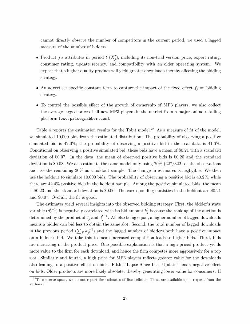
cannot directly observe the number of competitors in the current period, we used a lagged
measure of the number of bidders.
� Product j�s attributes in period t (Xtj); including its non-trial version price, expert rating,
consumer rating, update recency, and compatibility with an older operating system. We
expect that a higher quality product will yield greater downloads thereby a¤ecting the bidding
strategy.
� An advertiser speci�c constant term to capture the impact of the �xed e¤ect fj on bidding
strategy.
� To control the possible e¤ect of the growth of ownership of MP3 players, we also collectthe average lagged price of all new MP3 players in the market from a major online retailing
platform (www.pricegrabber.com).
Table 4 reports the estimation results for the Tobit model.28 As a measure of �t of the model,
we simulated 10,000 bids from the estimated distribution. The probability of observing a positive
simulated bid is 42:0%; the probability of observing a positive bid in the real data is 41:6%.
Conditional on observing a positive simulated bid, these bids have a mean of $0:21 with a standard
deviation of $0:07. In the data, the mean of observed positive bids is $0:20 and the standard
deviation is $0:08. We also estimate the same model only using 70% (227=322) of the observations
and use the remaining 30% as a holdout sample. The change in estimates is negligible. We then
use the holdout to simulate 10,000 bids. The probability of observing a positive bid is 40:2%; while
there are 42:4% positive bids in the holdout sample. Among the positive simulated bids, the mean
is $0:23 and the standard deviation is $0:06. The corresponding statistics in the holdout are $0:21
and $0:07. Overall, the �t is good.
The estimates yield several insights into the observed bidding strategy. First, the bidder�s state
variable (dt�1j ) is negatively correlated with its bid amount btj because the ranking of the auction is
determined by the product of btj and dt�1j . All else being equal, a higher number of lagged downloads
means a bidder can bid less to obtain the same slot. Second, the total number of lagged downloads
in the previous period (P
j0 dt�1j0 ) and the lagged number of bidders both have a positive impact
on a bidder�s bid. We take this to mean increased competition leads to higher bids. Third, bids
are increasing in the product price. One possible explanation is that a high priced product yields
more value to the �rm for each download, and hence the �rm competes more aggressively for a top
slot. Similarly and fourth, a high price for MP3 players re�ects greater value for the downloads
also leading to a positive e¤ect on bids. Fifth, �Lapse Since Last Update� has a negative e¤ect
on bids. Older products are more likely obsolete, thereby generating lower value for consumers. If
28To conserve space, we do not report the estimates of �xed e¤ects. These are available upon request from theauthors.
27

Table 4: Bidding Function Estimates
Median 95% Interval'Lagged Downloadsjt/103 �0:12� (�0:16;�0:09)Total Lagged Downloadst/103 0:04� (0:01; 0:08)Lagged Number of Bidderst 0:04� (0:01; 0:06)Lapse Since Last Updatejt �0:31� (�0:70;�0:02)Non-trial Version Pricejt 0:36� (0:33; 0:39)Expert Ratingsjt 0:47 (�0:26; 1:23)Consumer Ratingsjt 0:81� (0:10; 1:50)Compatibility Indexjt �0:91� (�1:74;�0:20)Lagged MP3 Player Pricet 0:03� (0:02; 0:03)
� 8:14� (6:78; 11:37)Log Marginal Likelihood �1123:59
this is the case, �rms can reasonably expect fewer �nal purchases after downloads and, therefore,
bid less for these products. Likewise and sixth, higher compatibility with prior software versions
re�ects product age leading to a negative estimate for this variable. Finally, ratings from consumers
and experts (albeit not signi�cant for experts) have a positive correlation with bid amounts �these
again imply greater consumer value for the goods, making it more pro�table to advertise them.
6.1.2 Consumer Model
The consumer model is estimated using MCMC approach based on the posterior distribution de-
scribed in Appendix A.1.2. We consider the download decisions for each of the 21 products who
entered auctions, plus the top 3 products who did not. Together these �rms constitute over 80%
of all downloads. The remaining number of downloads are scattered across 370 other �rms, each of
whom has a negligible share. Hence, we exclude them from our analysis.
Table 5: Alternative Numbers of Latent Segments
Log Marginal Likelihood1 Segment �12769:32 Segments� �12511:93 Segments �12571:14 Segments �12551:4Note: * indicates the model with the best �t.
We calibrate the model by estimating an increasing number of latent segments until there is
no signi�cant improvement in model �t. We use log marginal likelihood as the measurement for
model �t. In Table 5 we report the comparison of the log marginal likelihoods for models with up
28
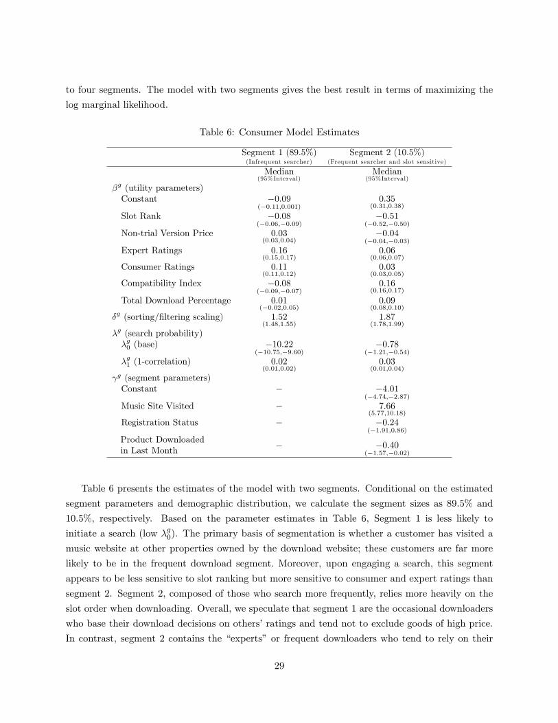
to four segments. The model with two segments gives the best result in terms of maximizing the
log marginal likelihood.
Table 6: Consumer Model Estimates
Segment 1 (89:5%)(Infrequent searcher)
Segment 2 (10:5%)(Frequent searcher and slot sensitive)
Median(95%Interval)
Median(95%Interval)
�g (utility parameters)Constant �0:09
(�0:11;0:001)0:35
(0:31;0:38)
Slot Rank �0:08(�0:06;�0:09)
�0:51(�0:52;�0:50)
Non-trial Version Price 0:03(0:03;0:04)
�0:04(�0:04;�0:03)
Expert Ratings 0:16(0:15;0:17)
0:06(0:06;0:07)
Consumer Ratings 0:11(0:11;0:12)
0:03(0:03;0:05)
Compatibility Index �0:08(�0:09;�0:07)
0:16(0:16;0:17)
Total Download Percentage 0:01(�0:02;0:05)
0:09(0:08;0:10)
�g (sorting/�ltering scaling) 1:52(1:48;1:55)
1:87(1:78;1:99)
�g (search probability)�g0 (base) �10:22
(�10:75;�9:60)�0:78
(�1:21;�0:54)�g1 (1-correlation) 0:02
(0:01;0:02)0:03
(0:01;0:04)
g (segment parameters)Constant � �4:01
(�4:74;�2:87)Music Site Visited � 7:66
(5:77;10:18)
Registration Status � �0:24(�1:91;0:86)
Product Downloadedin Last Month
� �0:40(�1:57;�0:02)
Table 6 presents the estimates of the model with two segments. Conditional on the estimated
segment parameters and demographic distribution, we calculate the segment sizes as 89:5% and
10:5%, respectively. Based on the parameter estimates in Table 6, Segment 1 is less likely to
initiate a search (low �g0). The primary basis of segmentation is whether a customer has visited a
music website at other properties owned by the download website; these customers are far more
likely to be in the frequent download segment. Moreover, upon engaging a search, this segment
appears to be less sensitive to slot ranking but more sensitive to consumer and expert ratings than
segment 2. Segment 2, composed of those who search more frequently, relies more heavily on the
slot order when downloading. Overall, we speculate that segment 1 are the occasional downloaders
who base their download decisions on others�ratings and tend not to exclude goods of high price.
In contrast, segment 2 contains the �experts� or frequent downloaders who tend to rely on their
29
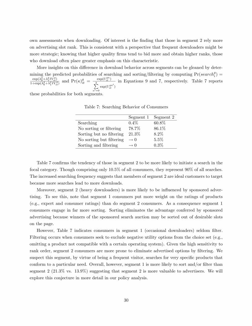
own assessments when downloading. Of interest is the �nding that those in segment 2 rely more
on advertising slot rank. This is consistent with a perspective that frequent downloaders might be
more strategic; knowing that higher quality �rms tend to bid more and obtain higher ranks, those
who download often place greater emphasis on this characteristic.
More insights on this di¤erence in download behavior across segments can be gleaned by deter-
mining the predicted probabilities of searching and sorting/�ltering by computing Pr(searchgi ) =exp(�g0+�
g1IV
git)
1+exp(�g0+�g1IV
git)and Pr(�)git =
exp(Ug�it )3P
�0=0exp(Ug�
0it )
in Equations 9 and 7, respectively. Table 7 reports
these probabilities for both segments.
Table 7: Searching Behavior of Consumers
Segment 1 Segment 2Searching 0:4% 60:8%No sorting or �ltering 78:7% 86:1%Sorting but no �ltering 21:3% 8:2%No sorting but �ltering ! 0 5:5%Sorting and �ltering ! 0 0:3%
Table 7 con�rms the tendency of those in segment 2 to be more likely to initiate a search in the
focal category. Though comprising only 10:5% of all consumers, they represent 90% of all searches.
The increased searching frequency suggests that members of segment 2 are ideal customers to target
because more searches lead to more downloads.
Moreover, segment 2 (heavy downloaders) is more likely to be in�uenced by sponsored adver-
tising. To see this, note that segment 1 consumers put more weight on the ratings of products
(e.g., expert and consumer ratings) than do segment 2 consumers. As a consequence segment 1
consumers engage in far more sorting. Sorting eliminates the advantage conferred by sponsored
advertising because winners of the sponsored search auction may be sorted out of desirable slots
on the page.
However, Table 7 indicates consumers in segment 1 (occasional downloaders) seldom �lter.
Filtering occurs when consumers seek to exclude negative utility options from the choice set (e.g.,
omitting a product not compatible with a certain operating system). Given the high sensitivity to
rank order, segment 2 consumers are more prone to eliminate advertised options by �ltering. We
suspect this segment, by virtue of being a frequent visitor, searches for very speci�c products that
conform to a particular need. Overall, however, segment 1 is more likely to sort and/or �lter than
segment 2 (21:3% vs. 13:9%) suggesting that segment 2 is more valuable to advertisers. We will
explore this conjecture in more detail in our policy analysis.
30

6.2 Second Step Estimation Results
6.2.1 Alternative Models
In addition to our proposed model, we consider two alternative models of seller behavior: i) myopic
bidding and ii) heterogeneous valuations across consumer segments.29 Table 8 reports the �t of
each model. In the �rst alternative model, advertisers maximize period pro�ts independently
as opposed to solving the dynamic bidding problem given in Equation 19. This model yields
a considerably poorer �t. Hence, we conclude that advertisers are bidding strategically. This
strategic behavior might result from dynamics in the bidding process coupled with non-linearities
in advertising response. Similar dynamic behavior has been evidenced in the face of non-linear
advertising demand systems with dynamics in advertising carryover (Bronnenberg (1998)).
The second model considers the case wherein advertiser valuations for clicks di¤er across seg-
ments. In this model, we augment Equation 16 by allowing it to vary by segment and then integrate
this heterogeneity into the seller pro�t function given by Equation 17. This model leads to only
a negligible increase in �t. Closer inspection of the results indicates little di¤erence in valuations
across segments, implying advertisers perceive that the conversion rates of each segment are es-
sentially the same. Hence, we adopt the more parsimonious single valuation model. It is further
worth noting that all of our subsequent results and policy simulations evidence essentially no change
across these two models.
Table 8: Alternative Models
Model Log Marginal LikelhoodBase Model �1651:3Base Model Without Advertiser Dynamics �1701:3Base Model With Heterogeneous Customer Valuations �1645:1
6.2.2 Valuation Model Results
Table 9 shows the results of second step estimation for the favored model.30 With respect to
the advertiser value function, we �nd that newer, more expensive and better rated products yield
greater values to the advertiser. This is consistent with our conjecture in Section 6.1.1 that �rms
bid more aggressively when having higher values for downloads. We �nd that, after controlling for
observed product characteristics, 95% of the variation in valuations across �rms is on the order of
$0:02. We attribute this variation in part due to di¤erences in the operating e¢ ciency of the �rms.
29We do not estimate the discount factor �. As shown in Rust (1994), the discount factor is usually unidenti�ed.We �x � = 0:95 for our estimation. We also experiment at � = 0:90 and see minimal di¤erence in the results.30Advertiser speci�c constant terms fj are not reported to save space.
31

Table 9: Value per Click Parameter Estimates
Median 95% Interval�Lapse Since Last Updatejt �0:98� (�1:02;�0:95)Non-trial Version Pricejt 0:24� (0:23; 0:25)Expert Ratingsjt 0:46� (0:38; 0:65)Consumer Ratingsjt 0:97� (0:94; 0:98)Compatibility Indexjt �0:27� (�0:29;�0:26)Lagged MP3 Player Pricet 0:01� (0:01; 0:02)
, random shock std. dev. 1:45� (1:43; 1:51)
Log Marginal Likelihood �1651:33
Figure 4: Distribution of Values per Download
32
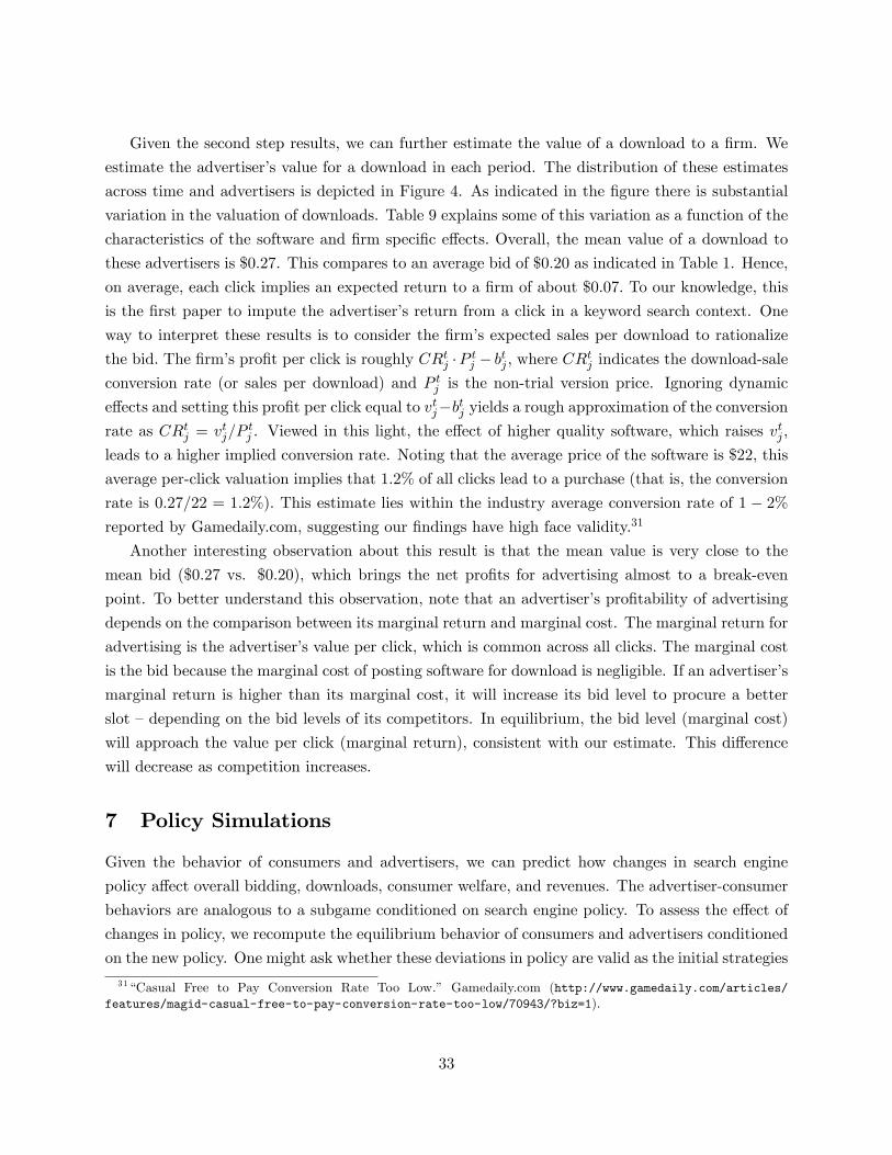
Given the second step results, we can further estimate the value of a download to a �rm. We
estimate the advertiser�s value for a download in each period. The distribution of these estimates
across time and advertisers is depicted in Figure 4. As indicated in the �gure there is substantial
variation in the valuation of downloads. Table 9 explains some of this variation as a function of the
characteristics of the software and �rm speci�c e¤ects. Overall, the mean value of a download to
these advertisers is $0:27. This compares to an average bid of $0:20 as indicated in Table 1. Hence,
on average, each click implies an expected return to a �rm of about $0:07: To our knowledge, this
is the �rst paper to impute the advertiser�s return from a click in a keyword search context. One
way to interpret these results is to consider the �rm�s expected sales per download to rationalize
the bid. The �rm�s pro�t per click is roughly CRtj �P tj � btj ; where CRtj indicates the download-saleconversion rate (or sales per download) and P tj is the non-trial version price. Ignoring dynamic
e¤ects and setting this pro�t per click equal to vtj�btj yields a rough approximation of the conversionrate as CRtj = vtj=P
tj . Viewed in this light, the e¤ect of higher quality software, which raises v
tj ,
leads to a higher implied conversion rate. Noting that the average price of the software is $22, this
average per-click valuation implies that 1:2% of all clicks lead to a purchase (that is, the conversion
rate is 0:27=22 = 1:2%). This estimate lies within the industry average conversion rate of 1 � 2%reported by Gamedaily.com, suggesting our �ndings have high face validity.31
Another interesting observation about this result is that the mean value is very close to the
mean bid ($0:27 vs. $0:20), which brings the net pro�ts for advertising almost to a break-even
point. To better understand this observation, note that an advertiser�s pro�tability of advertising
depends on the comparison between its marginal return and marginal cost. The marginal return for
advertising is the advertiser�s value per click, which is common across all clicks. The marginal cost
is the bid because the marginal cost of posting software for download is negligible. If an advertiser�s
marginal return is higher than its marginal cost, it will increase its bid level to procure a better
slot �depending on the bid levels of its competitors. In equilibrium, the bid level (marginal cost)
will approach the value per click (marginal return), consistent with our estimate. This di¤erence
will decrease as competition increases.
7 Policy Simulations
Given the behavior of consumers and advertisers, we can predict how changes in search engine
policy a¤ect overall bidding, downloads, consumer welfare, and revenues. The advertiser-consumer
behaviors are analogous to a subgame conditioned on search engine policy. To assess the e¤ect of
changes in policy, we recompute the equilibrium behavior of consumers and advertisers conditioned
on the new policy. One might ask whether these deviations in policy are valid as the initial strategies
31�Casual Free to Pay Conversion Rate Too Low.� Gamedaily.com (http://www.gamedaily.com/articles/features/magid-casual-free-to-pay-conversion-rate-too-low/70943/?biz=1).
33

might re�ect optimal behavior on the part of the search engine. However, extensive interactions
with the search site makes it clear that they have neither considered using these alternative policies
nor have they tried them in the past in order to obtain a sense of the strategies�impacts. Hence, it
is hard to argue that they are behaving strategically and thus we think these are reasonable policy
simulations to consider. Alternatively, estimating a model incorporating the engine�s behavior
invokes rather strong assumptions of rationality due to the complexity and novelty of the problem.
Also, we observe no variation in the considered behaviors of the search engine, meaning there is no
means to identify the primitives driving such behaviors.
We describe four policy simulations: i) the e¤ect of alternative webpage designs on search
engine revenues, ii) the value of targeting (i.e., not only allowing advertisers to bid on keywords
but also on market segments.), iii) the value of disaggregate consumer data, and iv) the e¤ect of
alternative pricing mechanisms on search engine revenue. As we can no longer assume the optimal
policy estimated in stage one of our two-step estimator remains valid in the face of a change
in search engine policy, the following policy simulations involve explicitly solving the dynamic
programming problem. Though an involving task, recent advances pertaining to approximate
dynamic programming makes solving high-dimension DP problems become possible (Powell (2007)).
More details regarding the implementation of the policy simulations are presented in Appendix C.
Hence, we limit our discussion to the objectives and insights from these simulations.
7.1 Policy Simulation I: Alternative Webpage Design
The goal of the search engine�s sorting/�ltering options is to provide consumers with easier access
to price and rating information across di¤erent products. As shown in section 4.1 and evidenced
by our results, sorting and �ltering play a crucial role in consumer decision process. In light
of this outcome, it is possible to consider an alternative webpage design of the search engine �
eliminating the option of sorting and �ltering for consumers �and assessing the resulting impact
on consumer search, advertiser bidding, and the search engine�s revenues. Because this change can
have contrasting e¤ects on consumer behavior (consumer should be less likely to search on the
site because of the decrease in utility arising from fewer search options) and advertiser behavior
(advertisers should bid more because of the decreased likelihood their advertisements will be sorted
or �ltered o¤ of the search results), the overall e¤ect is unclear. Using our model, it can be
tested which e¤ect dominates. We do this by setting the probability of consumer choosing no
sorting/�ltering option in equation 7 as 1. This manipulation mimics the scenario in which the
sorting/�ltering option is disabled. Under this new policy, we �nd that the search engine�s revenue
decreases by 3:7%, suggesting the consumer e¤ect is larger.
Next, to more precisely measure these contrasting e¤ects, we apportion the revenue change
across consumers and advertisers. Let Dtj0 (D
tj1) denote the number of downloads for product j in
period t before (after) the change of the webpage. Let Btj0 (B
tj1) denote the bid from advertiser j
34
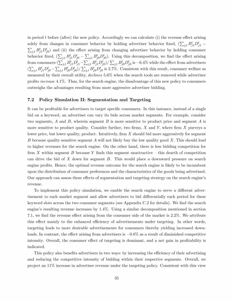
in period t before (after) the new policy. Accordingly we can calculate (i) the revenue e¤ect arising
solely from changes in consumer behavior by holding advertiser behavior �xed, (P
j;tBtj1D
tj1 �P
j;tBtj1D
tj0) and (ii) the e¤ect arising from changing advertiser behavior by holding consumer
behavior �xed, (P
j;tBtj1D
tj0 �
Pj;tB
tj0D
tj0). Using this decomposition, we �nd the e¤ect arising
from consumers (P
j;tBtj1D
tj1�
Pj;tB
tj1D
tj0)=
Pj;tB
tj0D
tj0 is �6:4% while the e¤ect from advertisers
(P
j;tBtj1D
tj0�
Pj;tB
tj0D
tj0)=
Pj;tB
tj0D
tj0 is 2:7%. Consistent with this result, consumer welfare as
measured by their overall utility, declines 5:6% when the search tools are removed while advertiser
pro�ts increase 4:1%. Thus, for the search engine, the disadvantage of this new policy to consumers
outweighs the advantages resulting from more aggressive advertiser bidding.
7.2 Policy Simulation II: Segmentation and Targeting
It can be pro�table for advertisers to target speci�c consumers. In this instance, instead of a single
bid on a keyword, an advertiser can vary its bids across market segments. For example, consider
two segments, A and B; wherein segment B is more sensitive to product price and segment A is
more sensitive to product quality. Consider further, two �rms, X and Y; where �rm X purveys a
lower price, but lower quality, product. Intuitively, �rm X should bid more aggressively for segment
B because quality sensitive segment A will not likely buy the low quality good X. This should lead
to higher revenues for the search engine. On the other hand, there is less bidding competition for
�rm X within segment B because Y �nds this segment unattractive �this dearth of competition
can drive the bid of X down for segment B. This would place a downward pressure on search
engine pro�ts. Hence, the optimal revenue outcome for the search engine is likely to be incumbent
upon the distribution of consumer preferences and the characteristics of the goods being advertised.
Our approach can assess these e¤ects of segmentation and targeting strategy on the search engine�s
revenue.
To implement this policy simulation, we enable the search engine to serve a di¤erent adver-
tisement to each market segment and allow advertisers to bid di¤erentially each period for these
keyword slots across the two consumer segments (see Appendix C.2 for details). We �nd the search
engine�s resulting revenue increases by 1:4%. Using a similar decomposition mentioned in section
7.1, we �nd the revenue e¤ect arising from the consumer side of the market is 2:2%. We attribute
this e¤ect mainly to the enhanced e¢ ciency of advertisements under targeting. In other words,
targeting leads to more desirable advertisements for consumers thereby yielding increased down-
loads. In contrast, the e¤ect arising from advertisers is �0:8% as a result of diminished competitiveintensity. Overall, the consumer e¤ect of targeting is dominant, and a net gain in pro�tability is
indicated.
This policy also bene�ts advertisers in two ways: by increasing the e¢ ciency of their advertising
and reducing the competitive intensity of bidding within their respective segments. Overall, we
project an 11% increase in advertiser revenue under the targeting policy. Consistent with this view
35

of consumer gains, consumer welfare increases by 2:9%: In sum, every agent �nds this new policy
to be an improvement.
7.3 Policy Simulation III: Incorporating Disaggregate Level Data
Advertisers and search engines are endowed with di¤erent levels of information. The search engine
knows all of the clicks made by visitors to its site. The advertiser knows only the total number
of downloads all the advertisers received. Hence, there is an information asymmetry arising from
the di¤erent level of market intelligence accruing to each respective agent. Given this disaggregate
consumer information is owned by the search engine but not observed by advertisers, it is relevant to
ask how the information revelation from the platform to advertisers will a¤ect advertiser behavior
and, hence, platform revenues. In practice, this means that the platform is interested in whether
to sell or give this information to advertisers and how it should be priced. More generally, this
counterfactual exempli�ed the value of market intelligence and how it can be computed in the
context of a structural model.
Accordingly, we implement a counterfactual scenario under which advertisers have access to the
click histories of consumers similar to that described in Section 7.2, except that advertisers are not
able to bid by segment. We then assess i) how bidding behavior and returns to advertisers change
under this counterfactual information structure and ii) how the resulting revenues change at the
search engine. We �nd little change in bidding behavior, and that search engine pro�ts increase
only 0:08%. The �nding suggests that advertisers are able to form consistent inferences about
consumer behavior from the aggregate download behavior. The �nding is interesting because it
suggests there is little value to selling this information to advertisers and that aggregate data can
be useful for making inferences about consumer heterogeneity (Chen and Yang (2007), Musalem
et al. (2008)). Further, the result suggests the value of this disaggregate information lies not in the
more e¢ cient estimates, but rather in the ability to exploit this heterogeneity by targeting bids by
segment as outlined in Section 7.2.
7.4 Policy Simulation IV: Alternative Auction Mechanisms
Auction mechanism design has been an active domain of research since the seminal work of Vickrey
(1961). Optimal mechanism design involves several aspects including the rules of the auction, the
e¢ ciency of the auction in terms of allocation surplus across players, and so forth. We focus on the
payment rules in this investigation. In particular, while the focal search engine currently charges
winning advertisers their own bids, many major search engines such as Google.com and Yahoo.com
are applying a �generalized second-price auction�as termed in Edelman et al. (2007). Under the
generalized second-price auction rules, winners are still determined by the ranking of fbtj0dt�1j0 g8j0 .
However, instead of paying its own bid amount, the winner of a slot pays the highest losing bidder�s
36

bid adjusted by their last period downloads.32 For example, suppose bidder j wins a slot with the
bid of btj and last period download dt�1j ; its payment for each download will be btj0d
t�1j0 =dt�1j , where
j0 is the highest losing bidders for the slot bidder j wins.
Though �generalized second-price auction� is widely adopted by major search engines, the
optimality of such a mechanism has not been substantiated (Iyengar and Kumar (2006), Katona
and Sarvary (2008)). By implementing a policy simulation that contrasts the search engine and
advertiser revenues under the two di¤erent mechanisms, we �nd little di¤erence in revenues for
the advertiser or search engine (for example, search engine revenues increase 0:01%). However, the
advertisers�bids for clicks approach their values for clicks. Under second price auction, the median
ratio of bid/value is 0:97 compared to 0:78 under �rst price auction. This is consistent with the
theory that in equilibrium bidders bid their true values under �generalized second-price auction�
(Edelman et al. (2007)). This o¤ers empirical support for the contention that generalized second
price auctions yield truth telling �though we �nd little practical consequence in terms of auction
house revenue.
8 Conclusion
Given the $9B �rms annually spend on keyword advertising and its rapid growth, we contend
that the topic is of central concern to advertisers and platforms that host advertising alike. In
light of this growth, it is surprising that there is little extant empirical research pertaining to
modeling the demand and pricing for keyword advertising in an integrated fashion across advertisers,
searchers, and search engines. As a result, we develop a dynamic structural model of advertiser
bidding behavior coupled with an attendant model of search behavior. The interplay of these two
agents has a number of implications for the search engine platform that hosts them. Because we
need to infer advertiser and consumer valuations and use these estimates to infer the e¤ects of
a change in search engine strategy, we develop a structural model of keyword search as a two-
sided network. In particular, we consider i) how the platform or search engine should price its
advertising via alternative auction mechanisms, ii) whether the platform should accommodate
targeted bidding wherein advertisers bid not only on keywords, but also behavioral segments (e.g.,
those that purchase more often), iii) whether and how the search engine should sell information on
individual clicking histories, and iv) how an alternative webpage design of the search engine with
less product information would a¤ect bidding behavior and the engine�s revenues.
Our model of advertiser bidding behavior is predicated on the advertiser choosing its bids to
maximize the net present value of its discounted pro�ts. The period pro�ts contain two components:
i) the advertiser�s value for a given click times the number of clicks on the advertisement and ii)
the payment in form of the bid per click times the number of clicks on the advertisement. Whereas
32 In the paper by Edelman et al. (2007), the adjustment using last period downloads is not considered.
37
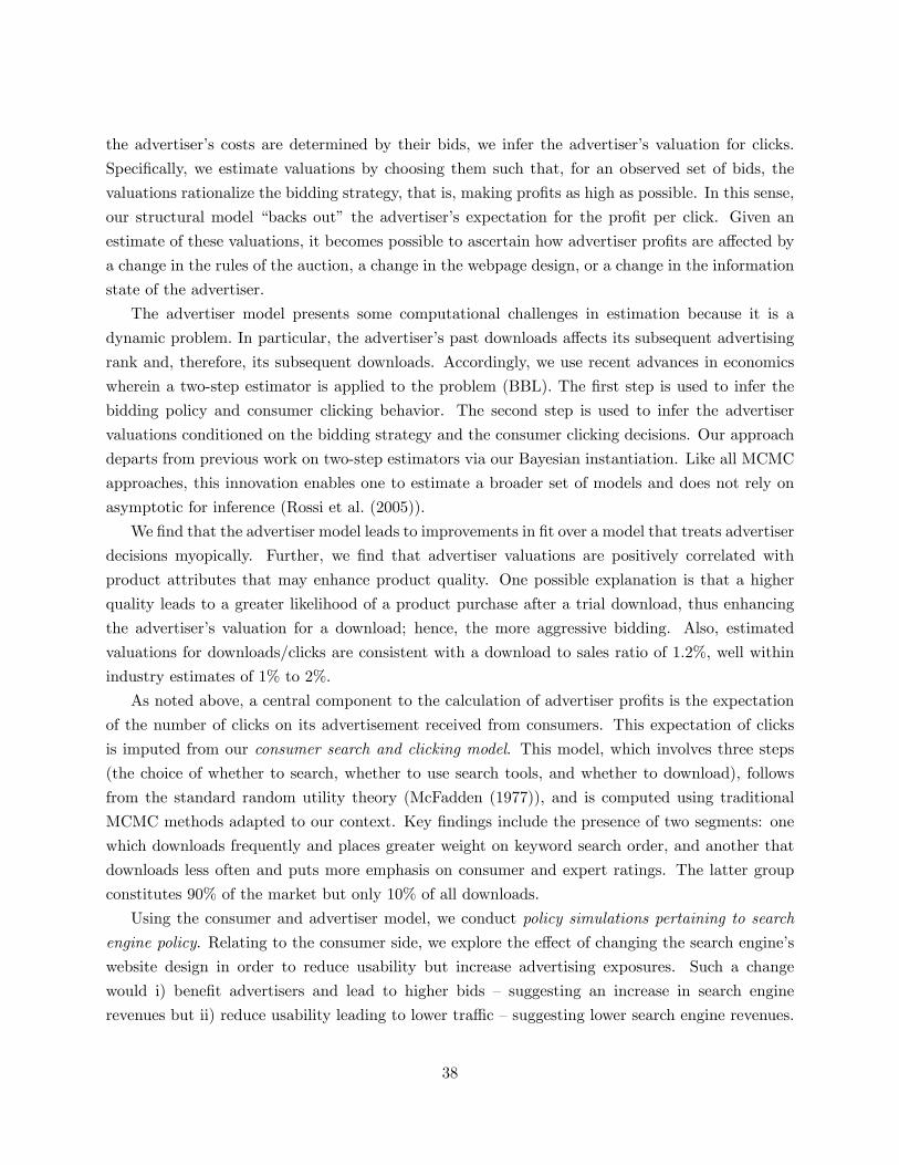
the advertiser�s costs are determined by their bids, we infer the advertiser�s valuation for clicks.
Speci�cally, we estimate valuations by choosing them such that, for an observed set of bids, the
valuations rationalize the bidding strategy, that is, making pro�ts as high as possible. In this sense,
our structural model �backs out� the advertiser�s expectation for the pro�t per click. Given an
estimate of these valuations, it becomes possible to ascertain how advertiser pro�ts are a¤ected by
a change in the rules of the auction, a change in the webpage design, or a change in the information
state of the advertiser.
The advertiser model presents some computational challenges in estimation because it is a
dynamic problem. In particular, the advertiser�s past downloads a¤ects its subsequent advertising
rank and, therefore, its subsequent downloads. Accordingly, we use recent advances in economics
wherein a two-step estimator is applied to the problem (BBL). The �rst step is used to infer the
bidding policy and consumer clicking behavior. The second step is used to infer the advertiser
valuations conditioned on the bidding strategy and the consumer clicking decisions. Our approach
departs from previous work on two-step estimators via our Bayesian instantiation. Like all MCMC
approaches, this innovation enables one to estimate a broader set of models and does not rely on
asymptotic for inference (Rossi et al. (2005)).
We �nd that the advertiser model leads to improvements in �t over a model that treats advertiser
decisions myopically. Further, we �nd that advertiser valuations are positively correlated with
product attributes that may enhance product quality. One possible explanation is that a higher
quality leads to a greater likelihood of a product purchase after a trial download, thus enhancing
the advertiser�s valuation for a download; hence, the more aggressive bidding. Also, estimated
valuations for downloads/clicks are consistent with a download to sales ratio of 1:2%, well within
industry estimates of 1% to 2%.
As noted above, a central component to the calculation of advertiser pro�ts is the expectation
of the number of clicks on its advertisement received from consumers. This expectation of clicks
is imputed from our consumer search and clicking model. This model, which involves three steps
(the choice of whether to search, whether to use search tools, and whether to download), follows
from the standard random utility theory (McFadden (1977)), and is computed using traditional
MCMC methods adapted to our context. Key �ndings include the presence of two segments: one
which downloads frequently and places greater weight on keyword search order, and another that
downloads less often and puts more emphasis on consumer and expert ratings. The latter group
constitutes 90% of the market but only 10% of all downloads.
Using the consumer and advertiser model, we conduct policy simulations pertaining to search
engine policy. Relating to the consumer side, we explore the e¤ect of changing the search engine�s
website design in order to reduce usability but increase advertising exposures. Such a change
would i) bene�t advertisers and lead to higher bids � suggesting an increase in search engine
revenues but ii) reduce usability leading to lower tra¢ c �suggesting lower search engine revenues.
38
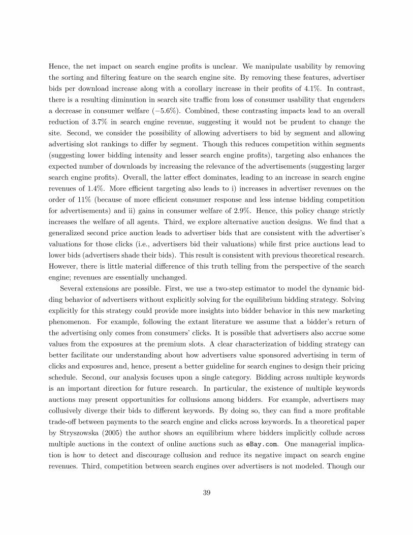
Hence, the net impact on search engine pro�ts is unclear. We manipulate usability by removing
the sorting and �ltering feature on the search engine site. By removing these features, advertiser
bids per download increase along with a corollary increase in their pro�ts of 4:1%. In contrast,
there is a resulting diminution in search site tra¢ c from loss of consumer usability that engenders
a decrease in consumer welfare (�5:6%). Combined, these contrasting impacts lead to an overallreduction of 3:7% in search engine revenue, suggesting it would not be prudent to change the
site. Second, we consider the possibility of allowing advertisers to bid by segment and allowing
advertising slot rankings to di¤er by segment. Though this reduces competition within segments
(suggesting lower bidding intensity and lesser search engine pro�ts), targeting also enhances the
expected number of downloads by increasing the relevance of the advertisements (suggesting larger
search engine pro�ts). Overall, the latter e¤ect dominates, leading to an increase in search engine
revenues of 1:4%. More e¢ cient targeting also leads to i) increases in advertiser revenues on the
order of 11% (because of more e¢ cient consumer response and less intense bidding competition
for advertisements) and ii) gains in consumer welfare of 2:9%. Hence, this policy change strictly
increases the welfare of all agents. Third, we explore alternative auction designs. We �nd that a
generalized second price auction leads to advertiser bids that are consistent with the advertiser�s
valuations for those clicks (i.e., advertisers bid their valuations) while �rst price auctions lead to
lower bids (advertisers shade their bids). This result is consistent with previous theoretical research.
However, there is little material di¤erence of this truth telling from the perspective of the search
engine; revenues are essentially unchanged.
Several extensions are possible. First, we use a two-step estimator to model the dynamic bid-
ding behavior of advertisers without explicitly solving for the equilibrium bidding strategy. Solving
explicitly for this strategy could provide more insights into bidder behavior in this new marketing
phenomenon. For example, following the extant literature we assume that a bidder�s return of
the advertising only comes from consumers�clicks. It is possible that advertisers also accrue some
values from the exposures at the premium slots. A clear characterization of bidding strategy can
better facilitate our understanding about how advertisers value sponsored advertising in term of
clicks and exposures and, hence, present a better guideline for search engines to design their pricing
schedule. Second, our analysis focuses upon a single category. Bidding across multiple keywords
is an important direction for future research. In particular, the existence of multiple keywords
auctions may present opportunities for collusions among bidders. For example, advertisers may
collusively diverge their bids to di¤erent keywords. By doing so, they can �nd a more pro�table
trade-o¤ between payments to the search engine and clicks across keywords. In a theoretical paper
by Stryszowska (2005) the author shows an equilibrium where bidders implicitly collude across
multiple auctions in the context of online auctions such as eBay.com. One managerial implica-
tion is how to detect and discourage collusion and reduce its negative impact on search engine
revenues. Third, competition between search engines over advertisers is not modeled. Though our
39

data provider has a dominant role in this speci�c category, inter-engine competition is unattended
in the literature. To some extent, sponsored search advertising can be understood as advertisers
purchasing products (media) from search engines through auctions. An advertiser makes discrete
choice about search engines before entering auctions. Little research has been done on the adver-
tiser�s choice problem, even though there is abundant discrete choice research that can be applied
(Palma et al. (1992)). Accordingly, the inter-engine competition deserves future attention. Finally,
our analysis is predicated on a relatively short duration of bidding behavior. Over the longer-term,
there may be additional dynamics in bidding and download behavior that might arise from con-
sumer learning or the penetration of search marketing into the market place, the so called �durable
goods problem,�(Horsky and Simon (1983)). Overall, we hope this study will inspire further work
to enrich our knowledge of this new marketplace.
40
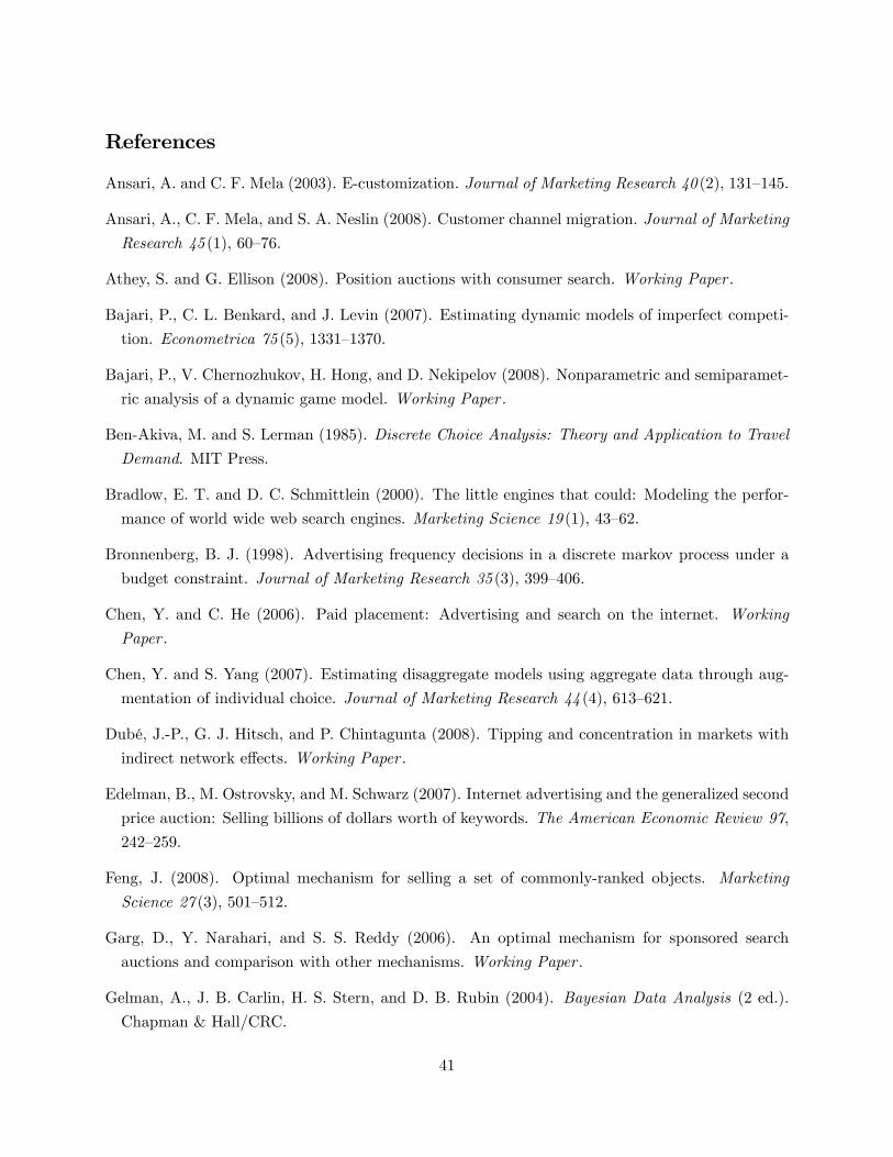
References
Ansari, A. and C. F. Mela (2003). E-customization. Journal of Marketing Research 40 (2), 131�145.
Ansari, A., C. F. Mela, and S. A. Neslin (2008). Customer channel migration. Journal of Marketing
Research 45 (1), 60�76.
Athey, S. and G. Ellison (2008). Position auctions with consumer search. Working Paper .
Bajari, P., C. L. Benkard, and J. Levin (2007). Estimating dynamic models of imperfect competi-
tion. Econometrica 75 (5), 1331�1370.
Bajari, P., V. Chernozhukov, H. Hong, and D. Nekipelov (2008). Nonparametric and semiparamet-
ric analysis of a dynamic game model. Working Paper .
Ben-Akiva, M. and S. Lerman (1985). Discrete Choice Analysis: Theory and Application to Travel
Demand. MIT Press.
Bradlow, E. T. and D. C. Schmittlein (2000). The little engines that could: Modeling the perfor-
mance of world wide web search engines. Marketing Science 19 (1), 43�62.
Bronnenberg, B. J. (1998). Advertising frequency decisions in a discrete markov process under a
budget constraint. Journal of Marketing Research 35 (3), 399�406.
Chen, Y. and C. He (2006). Paid placement: Advertising and search on the internet. Working
Paper .
Chen, Y. and S. Yang (2007). Estimating disaggregate models using aggregate data through aug-
mentation of individual choice. Journal of Marketing Research 44 (4), 613�621.
Dubé, J.-P., G. J. Hitsch, and P. Chintagunta (2008). Tipping and concentration in markets with
indirect network e¤ects. Working Paper .
Edelman, B., M. Ostrovsky, and M. Schwarz (2007). Internet advertising and the generalized second
price auction: Selling billions of dollars worth of keywords. The American Economic Review 97,
242�259.
Feng, J. (2008). Optimal mechanism for selling a set of commonly-ranked objects. Marketing
Science 27 (3), 501�512.
Garg, D., Y. Narahari, and S. S. Reddy (2006). An optimal mechanism for sponsored search
auctions and comparison with other mechanisms. Working Paper .
Gelman, A., J. B. Carlin, H. S. Stern, and D. B. Rubin (2004). Bayesian Data Analysis (2 ed.).
Chapman & Hall/CRC.
41

Ghose, A. and S. Yang (2007). An empirical analysis of search engine advertising: Sponsored search
in electronic markets. Working Paper .
Goldfarb, A. and C. Tucker (2008). Search engine advertising: Pricing ads to context. Working
Paper .
Greene, W. H. (2003). Econometric analysis. Prentice Hall.
Groves, T. (1979). E¢ cient collective choice when compensation is possible. The Review of Eco-
nomic Studies 46 (2), 227�241.
Horsky, D. and L. S. Simon (1983). Advertising and the di¤usion of new products. Marketing
Science 2 (1), 1�17.
Hotz, V. J. and R. A. Miller (1993). Conditional choice probabilities and the estimation of dynamic
models. The Review of Economic Studies 60 (3), 497�529.
Iyengar, G. and A. Kumar (2006). Characterizing optimal adword auctions. Working Paper .
Jofre-Bonet, M. and M. Pesendorfer (2003). Estimation of a dynamic auction game. Economet-
rica 71 (5), 1443�1489.
Judd, K. L. (1998). Numerical methods in economics. MIT Press.
Kamakura, W. A. and G. J. Russell (1989, November). A probabilistic choice model for market
segmentation and elasticity structure. Journal of Marketing Research 26 (4), 379�390.
Katona, Z. and M. Sarvary (2008). The race for sponsored links: A model of competition for search
advertising. Working Paper .
Krishna, V. (2002). Auction Theory. Academic Press.
McFadden, D. L. (1977). Modeling the choice of residential location. Cowles Foundation Discussion
Paper No. 477 .
Musalem, A., E. T. Bradlow, and J. S. Raju (2008). Who�s got the coupon? estimating consumer
preferences and coupon usage from aggregate information. Journal of Marketing Research 45 (6),
715�730.
Palma, A. D., S. P. Anderson, and J. F. Thisse (1992). Discrete Choice Theory of Product Di¤er-
entiation. Massachusetts Institute of Technology Press.
Pesendorfer, M. and P. Schmidt-Dengler (2008). Asymptotic least squares estimators for dynamic
games. Review of Economic Studies 75, 901�928.
42
Powell, W. B. (2007). Approximate Dynamic Programming: Solving the Curses of Dimensionality.
Wiley, Inc. Publication.
Qiu, F., Z. Liu, and J. Cho (2005). Analysis of user web tra¢ c with a focus on search activities. In
Proceedings of the International Workshop on the Web and Databases (WebDB), pp. 103�108.
Rochet, J.-C. and J. Tirole (2006). Two-sided markets: A progress report. Rand Journal of
Economics 37 (3), 645�667.
Rossi, P. E., G. M. Allenby, and R. E. McCulloch (2005). Bayesian statistics and marketing. John
Wiley and Sons.
Rust, J. (1994). Structural estimation of markov decision processes. In R. F. Engle and D. L.
McFadden (Eds.), Handbook of Econometrics, Volume IV. Amsterdam: Elsevier Science.
Rutz, O. J. and R. E. Bucklin (2007). A model of individual keyword performance in paid search
advertising. Working Paper .
Rutz, O. J. and R. E. Bucklin (2008). From generic to branded: A model of spillover dynamics in
paid search advertising. Working Paper .
Ryan, S. (2006). The costs of environmental regulation in a concentrated industry. Working Paper,
Massachusetts Institute of Technology .
Ryan, S. and C. Tucker (2008). Heterogeneity and the dynamics of technology adoption. Working
Paper, Massachusetts Institute of Technology .
Spiegelhalter, D. J., N. G. Best, W. R. Gilks, and H. Inskip (1996). Hepatitis b: a case study in
mcmc methods. In W. R. Gilks, S. Richardson, and D. J. Spiegelhalter (Eds.), Markov Chain
Monte Carlo in Practice, Chapter 2, pp. 21�43. Chapman & Hall/CRC.
Stryszowska, M. (2005). Simultaneous vs. overlapping internet auctions. Working Paper .
Train, K. (2003). Discrete Choice Methods with Simulation. Cambridge University Press.
Varian, H. R. (2007). Position auction. International Journal of Industrial Organization 25, 1163�
1178.
Vickrey, W. (1961). Counterspeculation, auctions, and competitive sealed tenders. Journal of
Finance 16 (1), 8�37.
Weitzman, M. L. (1979, May). Optimal search for the best alternative. Econometrica 47 (3),
641�654.
Yao, S. and C. F. Mela (2008). Online auction demand. Marketing Science 27 (5), 861�885.
43

Appendix
A Two Step Estimator
A.1 First Step Estimation
A.1.1 Estimating the Advertiser�s Policy Function
The Partial Policy Function The partial policy function links states (s) and characteristics
(X) to decisions (b). Ideally this relation can be captured by a relatively �exible parametric form
and estimated via methods such as maximum likelihood or MCMC to obtain the partial policy
function parameter estimates. The exact functional form is typically determined by model �t
comparison among multiple speci�cations (e.g., Jofre-Bonet and Pesendorfer (2003)). We consid-
ered several di¤erent speci�cations for the distribution of bids and found the truncated normal
distribution gives the best �t in terms of marginal likelihoods.33 Speci�cally, we allow
btj =
(yt�j0
if yt�j � �
otherwise(A1)
yt�j � N([st0;Xt0j ] � '+ 'j ; �2)
where [st0;Xt0j ] is the vector of independent variables; � is the standard deviation of y
�jt; 'j is
a bidder speci�c constant term due to the �xed e¤ect fj in valuations (Equation 16); � is the
truncation point, which is set at 15 to be consistent with the 15c/ minimum bid requirement of the
search engine.
One possible concern when estimating the partial policy function e� (s;X) (and the full policyfunction �
�s;X; rtj
�next) is that there may be multiple equilibrium strategies; and the observed
data are generated by multiple equilibria. If this were the case, the policy function would not lead
to a unique decision and would be of limited use in predicting advertiser behavior. It is therefore
necessary to invoke the following assumption (BBL).
Assumption 2 (Equilibrium Selection): The data are generated by a single Markov perfectequilibrium pro�le �.
Assumption 2 is relatively unrestrictive since our data is generated by auctions of one keyword and
from one search engine. Given data are from a single market, the likelihood is diminished that
di¤erent equilibria from di¤erent markets are confounded. We note that this assumption is often
employed in such contexts (e.g., Dubé et al. (2008)).
33We experimented with alternative speci�cations including a Beta distribution and a Weibull distribution whosescale, shape, and location parameters are functions of (s;X). The current speci�cation gives the best �t in terms ofmarginal likelihoods.
44

This partial policy function is then used to impute the full policy function bj = �j
�s;X; rtj
�as
detailed below based on rtj�s distribution parameter .
Full Policy Functions �tj�st;Xt;rtj
�: To evaluate the value function of this dynamic game, we
need to calculate bids as a function of not only (st;Xt) but also the unobserved shocks rtj (see
section 4.2.3). To infer this full policy function �j�st;Xt;rtj
�from the estimated partial policy
function, e�j(st;Xt), we introduce one additional assumption.
Assumption 3 (Monotone Choice): For each bidder j, its equilibrium strategy �j�st;Xt;rtj
�is increasing in rtj (BBL).
Assumption 3 implies that bidders who draw higher private valuation shocks rtj will bid more
aggressively.
To explore these two assumptions, note that the partial policy function e� �st;Xt�presents dis-
tributions for bid btj and the latent yt�j , whose CDF�s we denote as Fb
�btj jst;Xt
�and F
�yt�j jst;Xt
�,
respectively.34 According to the model in equation A1, the population mean of yt�j across bidders
and periods is [st;Xtj ] � '+ 'j . Around this mean, the variation across bidders and periods can be
captured by the variance term �2. With assumption 3, we can attribute �2 to the random shocks
rtj .
Given the normal distribution assumption of the random shock rtj � N�0; 2
�, we may impute
the yt�j (and hence btj) for each combination of
�st;Xt;rtj
�, i.e., the full policy function. To see this,
note that since �j�st;Xt;rtj
�is increasing in rtj ,
35
F�yt�j jst;Xt
�= Pr
��j�st;Xt;rtj
�� yt�j jst;Xt
�= �
���1j
�yt�j ; s
t;Xt�= �
where ��1j�yt�j ; s
t;Xt�is the inverse function of �j
�st;Xt;rtj
�with respect to rtj and �(�) is the
CDF of standard normal distribution. In equilibrium, we have �j�st;Xt;rtj
�= yt�j . By substitution
34To be more speci�c, we estimate a continuous distribution F�yt�j jst;Xt
�for yt�j from equation A1; then condi-
tional on the trunction point �, we can back out the (discontinuous) distribution Fb�btj jst;Xt
�for btj .
35 In this Appendix, we are abusing the notation of �j�st;Xt;rtj
�. For the purpose of a clear exposition, we de�ne
�j�st;Xt;rtj
�= btj in the paper. To match the bidding function estimated in equation A1, the more accurate de�nition
should be
btj =
�yt�j0
if yt�j � �otherwise
yt�j = �j�st;Xt;rtj
�:
45
and rearrangement we get
yt�j = �j�st;Xt;rtj
�(A2)
= F�1�����1j
�yt�j ; s
t;Xt�= �jst;Xt
�= F�1
���rtj=
�jst;Xt
�where ��1j
�yt�j ; s
t;Xt�= rtj ; r
tj= has a standard normal distribution.
Therefore there is a unique mapping between the likelihood of observing a given valuation shock
rtj and the yt�j . Each r
tj drawn by a �rm implies a corresponding quantile on the rtj�s distribution;
this quantile in turn implies a yt�j from the distribution represented by that �rm�s partial bidding
function e�j(st; Xt). However, because we do not know and, thus, the distribution of rtj , we have
to make draws from an alternative distribution rtj= that has a one-one quantile mapping to rtj .
To do this, we �rst draw a random shock rtj= from N(0; 1) for each advertiser i in period t. Next,
we determine F�yt�j jst;Xt
�using results estimated in Equation A1 and looking at the distribution
of its residuals to determine F . That is, for each value of yt�j ; we should be able to compute its
probability for a given st and Xt using F . Accordingly, F�1 links probabilities to yt�j (therefore btj)
for a given st and Xt. We then use F�1 to link the probability ��rtj=
�to btj for a particular s
t
and Xt. In this manner we ensure the bids and valuations in Equation A11 comport. In Appendix
A.2.1, when evaluating the value function for a set of given parameter values of in Equation A11
or evaluating base functions de�ned in Equation A12, we integrate out over the unobserved shocks
rtj by drawing many rtj= from N(0; 1).
A.1.2 Consumer Model Estimation
We derive the consumer model conditioned on the information state of the advertiser as described
in section 4.1. Given that advertisers do not observe what each person downloaded or the charac-
teristics of these persons, they must infer consumer behavior from aggregate instead of individual
level data.
Advertisers do observe the aggregate data in the form of download counts dtj = fdt1; dt2; :::; dtNgin period t. A single dtj follow a binomial distribution. Given the download probabilities P tj in
Equation 12, a single dtj�s probability mass function is
Mt
dtj
![P tj ]
dtj [1 � P tj ]Mt�dtj ; where Mt is
the consumer population size in period t. Hence the likelihood of observing dt is
L(dtjc) =Y
j
Mt
dtj
![P tj ]
dtj [1� P tj ]Mt�dtj
where c � f�g; �g; �g; g; �g0; �g1gg are parameters to be estimated.
46

Naturally, the full posterior distribution of the model will be the product of L(dtjc) acrossperiods and p(c), the prior distributions of parameters, i.e.,
p(cjdata) /Yt
L(dtjc) � p(c): (A3)
An advertiser�s predicted downloads dtj(k;Xtj ; c) can readily be constructed using the parame-
ter estimates as shown in equation 14
dtj(k;Xtj ; bc) =Mt
bP tj : (A4)
This prediction is then used to forecast expectations of future downloads and slot positions in the
�rm�s value function in the second step estimation.
A.1.3 State Transition Function P�s0 jbj ;b�j ; s;X
�To compute the state transition, note that the marginal number of expected downloads is given by
the expected downloads given a slot position multiplied by the probability of appearing in that slot
position and then summed across all positions:
P�s0 jbj ;b�j ; s;X
�=X
kd(k;X; c) Pr (kjbj ;b�j ; s;X) : (A5)
The expected downloads given a slot position in A5 is de�ned in 14. We can decompose the
likelihood of appearing in slot k as follows
Pr(kjbj ;b�j ; s;X) (A6)
= Prfk�Kg (kjbj ;b�j ; s;X) Ifk � Kg+ Prfk>Kg(kjbj ;b�j ; s;X)Ifk > Kg
where Prfk�Kg (kjbj ;b�j ; s;X) is the probability of appearing in slot k of the sponsored searchsection (i.e., k � K), and Prfk>Kg(kjbj ;b�j ; s;X) is the likelihood of appearing in slot k of theorganic search section (i.e., k > K). We discuss these two probabilities next.
Likelihood of Premium Slot k � K: Let us �rst consider the likelihood of winning one of
the premium slots k (k � K), Prfk�Kg (kjbj ;b�j ; s;X) as an order statistic re�ecting the relativequality of the advertiser�s bid, which is de�ned as bjd
(�1)j . Higher quality bids are more likely to be
assigned to better slots. Denote bd(bj0d(�1)j0 js;X) as the distribution CDF of bj0d(�1)j0 ,8j0, where
d(�1)j0 is from the state vector and bj0 has a distribution depending on the strategy pro�le � (�).36
For bidder j to win a premium slot k by bidding bj , it implies that (1) among all of the other N �136 It is di¢ cult to write a closed form solution for bd; but we may use the sample population distribution to
approximate bd.
47

competing bidders, there are k � 1 bidders who have a higher ranking than j in terms of bj0d(�1)j0
and (2) the other ones have a lower ranking than j. The probability of having a higher ranking
than j is [1 � bd(bjd(�1)j js;X)]. Thus the probability of bidder j winning slot k by bidding bj is
simply an order statistics as shown below; note that the combination
N � 1k � 1
!in the equation
is because any (k � 1) out of the (N � 1) competing bidders can have a higher ranking than j.37
Prfk�Kg (kjbj ;b�j ; s;X) (A7)
=
N � 1k � 1
![1�bd(bjd(�1)j js;X)]k�1[bd(bjd(�1)j js;X)](N�1)�(k�1)
=
N � 1k � 1
![1�bd(bjd(�1)j js;X)]k�1[bd(bjd(�1)j js;X)]N�k
Likelihood of Organic Slot k > K: Next we consider what happens when an advertiser does
not win this auction and is placed in the organic search section. In this case, by the rules of the
auction, the bidder�s slot is determined by its update recency compared to all products in the
organic search section. For bidder j to be placed in organic slot k > K it implies that (1) there
are K bidders who have a higher ranking of bj0d(�1)j0 than bidder j (i.e., j loses the auction) and
(2) among the other N �K � 1 products (i.e., all products at the search engine less those who winpremium slots and j itself), there are k �K � 1 products that have a higher update recency thanj and (3) the other ones have a lower ranking than j. Hence,
Prfk>Kg(kjbj ;b�j ; s;X)
= Pr(k > Kjbj ;b�j ; s;X) � Pr(kjbj ;b�j ; s;X; k > K) (A8)
where the �rst term is the probability of losing the auction (condition 1) and the second term
denotes the likelihood of appearing in position k > K (condition 2 and 3). Note that the main
reason for the di¤erence between A7 and A8 is the change of ranking mechanisms. The ranking
is based on bj0d(�1)j0 for k � K and update recency when k > K. The �rst term in A8 does not
appear as an order statistics (as shown below) since when k > K the order of bj0d(�1)j0 becomes
meaningless. Instead, the update recency is a¤ecting the ranking. The two terms in A8 can be
expressed as follows.
37An alternative interpretation of equation A7 is the probability mass function (PMF) of a binomial distribution.Among N � 1 competing bidders, there are k � 1 higher than bidder j and (N � 1)� (k � 1) lower than j, and theprobability of higher than j is [1�bd(bjd(�1)j js;X)]. Hence, we may consider the expression in A7 as the PMF of abinomial distribution.
48

Losing the auction implies that among j�s N � 1 opponents, there are K bidders who have a
higher ranking than j in terms of bj0d(�1)j0 . Hence,
Pr(k > Kjbj ;b�j ; s;X) = N � 1K
![1�bd(bjd(�1)j js;X)]K : (A9)
The conditional probability of being placed in an organic slot k > K (condition 2 and 3) is,
again, an order statistics.38 This distribution is incumbent upon the update recency of all N
products exclusive of the K winners in the sponsored search section. Denoting the distribution
of update recency of all products as up, which can be approximated from the sample population
distribution observed in the data, we obtain the following:
Pr(kjbj ;b�j ; s;X; k > K) (A10)
=
N �K � 1k �K � 1
![1�up]k�K�1[up](N�K�1)�(k�K�1)
=
N �K � 1k �K � 1
![1�up]k�K�1[up]N�k
Combining Equations A10 and A9 into A8, and then A8 and A7 into A6, yields the state
transition equation.
Given that we have detailed the estimation of the �rst step functions (�j�s;X; rtj
�, dtj(k;X
tj ; c);
P (s0jb; s;X)), we now turn to the second step estimator, which is incumbent upon these �rst stepfunctions.
A.2 Second Step Estimation of Bidder Model
In this Appendix we detail how to estimate the parameters in the value function. This is done in
two phases: �rst, we simulate the value function conditioned on a; and second, we construct the
likelihood using the simulated value function conditioned on a:
A.2.1 Phase 1: Simulation of Value Functions Given a
To construct the value function we �rst simplify its computation by linearization, and second using
this simpli�cation, we simulate the expected value function conditioned on a by integrating out
over draws for st, Xt, and ertj :38This order statistics can again be interpreted as the PMF of a binomial distribution similar to A7.
49

Linearize the Value Function We simplify the estimation procedure by relying on the fact
that Equation 17 is linear in the parameters a. We can rewrite Equation 17 by factoring out a.
E�j�bt; st;Xt; rtj ; a
�(A11)
=XK
k=1Pr�kjbtj ;bt�j ; st;Xt
�� (v(Xt
j ; �) + fj + rtj � btj) � dtj(k;Xt
j ; c)
+XN
k=K+1Pr�kjbtj ;bt�j ; st;Xt
�� (v(Xt
j ; �) + fj + rtj) � dtj(k;Xt
j ; c)
=
�XN
k=1Pr�kjbtj ;bt�j ; st;Xt
�� dtj(k;Xt
j ; c) �Xtj
�� �
+
�XN
k=1Pr�kjbtj ;bt�j ; st;Xt
�� dtj(k;Xt
j ; c)
�� fj
+
�XN
k=1Pr�kjbtj ;bt�j ; st;Xt
�� dtj(k;Xt
j ; c) � ertj� � �btj
XK
k=1Pr�kjbtj ;bt�j ; st;Xt
�dtj(k;X
tj ; c)
= Basetj1[�0; fj ]
0 +Basetj2 �Basetj3
where
Basetj1 �
24 PNk=1 Pr
�kjbtj ;bt�j ; st;Xt
�� dtj(k;Xt
j ; c) �XtjPN
k=1 Pr�kjbtj ;bt�j ; st;Xt
�� dtj(k;Xt
j ; c)
350 (A12)
Basetj2 ��XN
k=1Pr�kjbtj ;bt�j ; st;Xt
�� dtj(k;Xt
j ; c) � ertj�Basetj3 � btj
XK
k=1Pr�kjbtj ;bt�j ; st;Xt
�dtj(k;X
tj ; c)ertj = rtj= � N(0; 1):
Note that the values ofnBasetj1; Base
tj2; Base
tj3
o8tare conditionally independent of �; fj and
. This enables us to �rst evaluatenBasetj1; Base
tj2; Base
tj3
o8tand keep them constant when
drawing �; fj and from their posterior distributions. By doing so, we reduce the computational
burden of estimation as described next.
Simulate the Value Functions Given a: After the linearization, given a set of advertiser
parameters a = f�; fj=1;2;:::;N ; g and Equation A11, the value function depicted in Equation 19can also be written as the following with period index t invoked:
50

Vj�s0;X0;�; a
�= Es;X;r
" 1Xt=0
�t�j��; st;Xt; rtj ; a
�#(A13)
= E[1Xt=0
(�tBasetj1
"�
fj
#+Basetj2 �Basetj3)]
= [E1Xt=0
�tBasetj1]
"�
fj
#+ [E
1Xt=0
�tBasetj2] � [E1Xt=0
�tBasetj3]
where the expectation is taken over current and future private shocks, future states st, future Xt
and Rt.
An estimated value function bVj �s0;X0;�; a� can then be obtained by the following steps:1. Draw private shocks ertj from N(0; 1) for all bidders j in period 0; draw initial choice of s0
from the distribution of state variables derived from the observed data; draw X0 from the
observed distribution of product attributes.
2. Starting with the initial state s0, X0 and the ertj step 1, calculate bb0j for all bidders using theinversion (equation A2) described in Appendix A.1.1.
3. Use s0, X0 and bb0 to determine the slot ranking, whose distribution is Pr�kjbtj ;bt�j ; st;Xt�
in Equation A6 in Appendix A.1.3; using d(k;X0j ; c) in Equation 14, obtain a new state
vector s1, whose distribution is P (s1jbb0; s0;X0) in Equation A5 in Appendix A.1.3; draw X1from the observed distribution of product attributes.
4. Repeat step 1-3 for T periods for all bidders to compute all st, Xt, ertj , and bt for all periods;T is large enough so that the discount factor �T approaches 0.
5. Using st, Xt, ertj , dtj(k;Xtj ; c); and b
t, evaluatenBasetj1; Base
tj2; Base
tj3
ot=0;:::;T
and�[TPt=0
�tBasetj1]; [TPt=0
�tBasetj2]; [TPt=0
�tBasetj3]
�:
6. The resulting values of �Basetj1; Base
tj2; Base
tj3
t=0;:::;T
and ([TXt=0
�tBasetj1]; [TXt=0
�tBasetj2]; [TXt=0
�tBasetj3]
)
51

depend on the random draws of st;Xt; rt. To compute([E
1Xt=0
�tBasetj1]; [E1Xt=0
�tBasetj2]; [E1Xt=0
�tBasetj3]
);
repeat step 1-6 for NR times so as to integrate out over the draws. Note that when T is large
enough, [ETPt=0
�tBasetj�] is a good approximation of [E1Pt=0
�tBasetj�] since �T approaches 0.
7. Conditional on a set of parameters a and([E
1Xt=0
�tBasetj1]; [E1Xt=0
�tBasetj2]; [E1Xt=0
�tBasetj3]
);
we may evaluate bVj �s0;X0;�; a� from Equation A13.
An estimated deviation value function bVj �s0;X0;�0j ;��j ; a� with an alternative strategy �0jother than �j can be constructed by following the same procedure. We draw a deviated strategy
�0j by adding disturbance to the estimated policy function from Step 1. In particular, we add a
normally distributed random variable (mean = 0; s:d: = 0:3) to each parameter.
We implement this process by �rst drawingNS = 10 initial states for each bidder and fXtgt=0;1;:::;Tof all T = 200 periods. Then for each combination of bidder and initial state, we use this process
to compute the base value functions and ND = 100 perturbed base functions. In Step 6, we use
NR = 100. The discount factor � is �xed as 0:95.
The computational burden is reduced tremendously since we have linearized the value functions
and factored out the parameters a. We do not need to re-evaluate the value functions for each set
of parameters a. Instead, we only evaluate the base functions in Equation A12 once using step
1-6 and keep them �xed. Then for each draw of a from the posterior distribution we may evaluate
the value functions (step 7) so as to recover a as described below.
A.2.2 Phase 2: Recover a
Recall our goal is to assess the likelihood that 20 holds. De�ne Pj�s0(ns);X
0;�; �0j ; a�as the
probability of the event
nbVj(s0(ns);X0;�j ;��j ; a) � bVj(s0(ns);X0;�0j ;��j ; a)o ; (A14)
where s0(ns) stands for the ns-th initial state of bidder j. This event means that the estimated
value function for the given initial state s0(ns) with observed strategy �j is greater than the es-
timated value function with a deviation �0j . For observed data to be rational, we should have
52

Pj
�s0(ns);X
0;�; �0j ; a�converging to 1 under the true parameters, in the sense that all ND draws
should result in the event of equation A14.
Note that Pj�s0(ns);X
0;�; �0j ; a�is not observed, but it can be approximated with the sample
analog from the simulated ND draws of bVj(s0(ns); X0;�0j ; ��j ; a) as the follows:
bPj �s0(ns);X0;�; �0j ; a� (A15)
=1
ND
XND
nd=1InbVj(s0(ns);X0;�j ;��j ; a) � bVj(s0(ns);X0;�0j ;��j ; a)(nd)o
where the subscript (nd) indices the nd-th simulated bVj(s0(ns); X0;�0j ; ��j ; a).
By pooling together all bPj �s0(ns);X0;�; �0j ; a��s across bidders and (ns), we are able to con-struct a simulated likelihood function as the following
L =Y
j;(ns)bPj �s0(ns);X0;�; �0j ; a� : (A16)
Denoting the prior of a as p(a), the posterior can be written as
p(ajdata) /Y
j;(ns)bPj �s0(ns);X0;�; �0j ; a� p(a) (A17)
There may be some e¢ ciency loss by using Bayesian method in estimation since the di¤erences
between Vj(s0(ns); X0;�j ; ��j ; a) and Vj(s0(ns); X
0;�0j ; ��j ; a) also provide some information about
the estimates and are not utilized (BBL). However, Bayesian method provides desirable small
sample properties, increases statistical e¢ ciency, and enables the estimation of a wide array of
functional forms (Rossi et al. (2005)). We consider the bene�ts of Bayesian method to outweigh
the loss of e¢ ciency.
B Sampling Chain
B.1 Advertiser Model
B.1.1 Priors
To facilitate explication, denote the vector [st0;Xt0j ] � Ztj , the matrix [Z
tj ]8j;t � Z; and the vector
[yt�j ]8j;t � y�. We also denote the number of bidders as N and the number of observations for bidder
j as Nj . So the total number of observations isP
j Nj ; the dimension of Ztj is 1 by d (the dimension
of [st0; Xt0j ]); the dimension of Z is
Pj Nj by d; and the dimension of y� is
Pj Nj . The vector of
bidder speci�c �xed e¤ects, 'fe; is a column vector with a length of the number of bidders. � is a
matrix whose dimension isP
j Nj by N . Suppose rows a to b of matrix Z are the observations of
53

bidder j, then rows a to b of the j-th column of � are 1. Other elements of � are 0. Also denote
� � [�; Z], whose dimension isP
j Nj by (N + d).
The advertiser model is speci�ed as
btj =
(yt�j0
if yt�j � �
otherwise(A18)
yt�j � N([st0;Xt0j ] � '+ 'j ; �2):
We iterate the sampling chain for 20,000 and use the second half of the chain to make inference.
The priors use a di¤used variance of 100; examinations of the posteriors shows that the choice of
the variance is the order of magnitude greater than posterior distributions, which assures a proper
but di¤used prior (Spiegelhalter et al. (1996), Gelman et al. (2004)).
Priors Selected Value
' =['0; '1; :::; 'N ]0 ' � N
�'0; I'�
2'
�'0: estimates of a classical Tobit model of
bids on � = [�; Z] with the truncation at 15
�2' = 100
I' is an identity matrix with the dimension of
N + d
� � � TN(0;+1)(�� ; �2� ) �� = 5; �
2� = 100
B.1.2 Conditional Posteriors
� yt�jyt�j is determined by the following
yt�j = btj ; if btj > 0
yt�j � TN(�1;15](Ztj'+ 'j ; �
2); if btj = 0
yt�j is right truncated at 15 when btj = 0; this is consistent with the 15c/ minimum bid
requirement of the search engine.
54

� '
Prior ' � N�'0; I'�
2'
�(A19)
Likelihood L /Qj;texp(�
[yt�j � (Ztj'+ 'j)]2
2�2)
Posterior ('j�) � N(�';�')
�' = [�0���2 + ��2' ]�1
�' = �' � f�0 � y���2 +'0��2' g
� �Prior � � TN(0;+1)(�� ; �
2� )
A random walk proposal density is used in the (r)-th iteration, � (r) � TN(0;+1)(�(r�1); �2p),
where � (r�1) is the value from the (r � 1)-th iteration; �2p is the tuning variance which ischosen so that the acceptance rate is between 15%� 50%.
The acceptance probability pr� = min(1; pr) and
pr =L(� (r)j�)p(� (r)j�� ; �2� )�(� (r�1)j� (r); �2p)
L(� (r�1)j�)p(� (r�1)j�� ; �2� )�(� (r)j� (r�1); �2p)
where p(� (�)j�� ; �2� ) is the density of � (�) evaluated using the prior. L(� (�)j�) is the likelihoodevaluated at � (�). To be speci�c
L(� (�)j�) /Qj;t�(yt�j ;Z
tj'+ 'j ; �
(�))
where �(yt�j ;Ztj' + 'j ; �
(�)) is the normal density of yt�j evaluated with mean Ztj' + 'j and
standard deviation � (�).
55

B.2 Consumer Model
B.2.1 Priors
Priors Selected Value
Bg � ff�gjg08j ; f�gag08ag Bg � N
�0; IB � �2B
� IB is an identity matrix of dimension
product attributes and intercepts; �2B = 100
�g �g � TN(0;+1)(1; �2�) �2� = 100
�g0 �g0 � N(0; �2�) �2� = 100
�g1 �g1 � TN(0;1)(0:5; �2�) �2� = 100
g0 g0 � N(0; �2 ) �2 = 100
g g � N(0; I � �2 )I is an identity matrix of dimension
of 3; �2 = 100
B.2.2 Conditional Posteriors
� Bg = ff�gjg08j ; f�gag08ag
Prior Bg � N�0; IB � �2B
�A random walk proposal density is used in the (r)-th iteration, Bg(r) � N(Bg(r�1); �2pB),
where Bg(r�1) is the value from the (r � 1)-th iteration; �2pB is the tuning variance which ischosen so that the acceptance rate is between 15%� 50%.
The acceptance probability pr� = min(1; pr) and
pr =L(Bg(r)j�)p(Bg(r)j0; IB � �2B)
L(Bg(r�1)j�)p(Bg(r�1)j0; IB � �2B)
where p(Bg(�)j0; IB � �2B) is the density of Bg(�) evaluated using the prior. L(Bg(�)j�) is thelikelihood evaluated at Bg(�). To be speci�c
L(Bg(�)j�) /Y
j;t
Mt
dtj
![P tj ]
dtj [1� P tj ]Mt�dtj
where P tj is de�ned in equation 12 and evaluated at Bg(�). dtj is the actual downloads observed
in the data and Mt is the market size. We set this to the mean total monthly number of
visitors to the search engine and all other Internet properties owned by its parent (hence
Mt =M).
� �g
56

Prior �g � TN(0;+1)(1; �2�)
A random walk proposal density is used in the (r)-th iteration, �g(r) � TN(0;+1)(�g(r�1); �2p�).
The acceptance probability pr� = min(1; pr) and
pr =L(�g(r)j�)p(�g(r)j1; �2�)�(�
g(r�1)j�g(r); �2p�)L(�g(r�1)j�)p(�g(r�1)j1; �2�)�(�
g(r)j�g(r�1); �2p�)
where p(�g(�)j1; �2�) is the density of �g(�) evaluated using the prior. L(�g(�)j�) is the likelihood
evaluated at �g(�). �(�g(r�1)j�g(r); �2p�)=�(�g(r)j�g(r�1); �2p�) is the correction ratio since the
proposal density is asymmetric.
� �g0
Prior �g0 � N(0; �2�)
A random walk proposal density is used in the (r)-th iteration, �g(r)0 � N(�g(r�1)0 ; �2p�).
The acceptance probability pr� = min(1; pr) and
pr =L(�
g(r)0 j�)p(�g(r)0 j1; �2�)
L(�g(r�1)0 j�)p(�g(r�1)0 j1; �2�)
where p(�g(�)0 j1; �2�) is the density of �g(�)0 evaluated using the prior. L(�g(�)0 j�) is the likelihood
evaluated at �g(�)0 .
� �g1
Prior �g1 � TN(0;1)(0:5; �2�)
A random walk proposal density is used in the (r)-th iteration, �g(r)1 � TN(0;1)(�g(r�1)1 ; �2p�).
The acceptance probability pr� = min(1; pr) and
pr =L(�
g(r)1 j�)p(�g(r)1 j0:5; �2�)�(�
g(r�1)1 j�g(r)1 ; �2p�)
L(�g(r�1)1 j�)p(�g(r�1)1 j0:5; �2�)�(�
g(r)1 j�g(r�1)1 ; �2p�)
57

where p(�g(�)1 j1; �2�) is the density of �g(�)1 evaluated using the prior.39 L(�g(�)1 j�) is the likelihood
evaluated at �g(�)1 . �(�g(r�1)1 j�g(r)1 ; �2p�)=�(�g(r)1 j�g(r�1)1 ; �2p�) is the correction ratio since the
proposal density is asymmetric.
� g0
Prior g0 � N(0; �2 )
A random walk proposal density is used in the (r)-th iteration, g(r)0 � N( g(r�1)0 ; �2p ).
The acceptance probability pr� = min(1; pr) and
pr =L(
g(r)0 j�)p( g(r)0 j0; �2 )
L( g(r�1)0 j�)p( g(r�1)0 j0; �2 )
where p( g(�)0 j0; �2 ) is the density of g(�)0 evaluated using the prior. L( g(�)0 j�) is the likelihood
evaluated at g(�)0 .
� g
Prior g � N(0; I � �2 )
A random walk proposal density is used in the (r)-th iteration, g(r) � N( g(r�1); I � �2p ).
The acceptance probability pr� = min(1; pr) and
pr =L( g(r)j�)p( g(r)j0; I � �2 )
L( g(r�1)j�)p( g(r�1)j0; I � �2 )
where p( g(�)j0; I � �2 ) is the density of g(�) evaluated using the prior. L( g(�)j�) is thelikelihood evaluated at g(�).
B.3 Second Step Estimation
B.3.1 Priors
To facilitate explication denote the vector [�0; f1; f2; :::; fN ]0 as �.
39Note that �g1 is truncated to (0; 1) and has a large variance (100) for its prior. Hence, the prior is essentially anuninformative uniform distribution.
58

Priors Selected Value
� � � N��0; I��
2�
��0: a vector of zeros with the length of the
number of product attributes plus N , the
number of bidders
�2� = 100
I� is an identity matrix with the dimension
of the number of product attributes plus N
� TN(0;+1)(� ; �2 ) �0 = 1; �
2 = 100
B.3.2 Conditional Posteriors
� �Prior � � N
��0; I��
2�
�A random walk proposal density is used in the (r)-th iteration, �(r) � N(�(r�1); I��
2p�),
where �(r�1) is the value from the (r � 1)-th iteration; �2p� is a scalar and functions as thetuning variance.
The acceptance probability pr� = min(1; pr) and
pr =L(�(r)j�)p(�(r)j�0; I��2�)
L(�(r�1)j�)p(�(r�1)j�0; I��2�)
where p(�(�)j�0; I��2�) is the density of �(�) evaluated using the prior. L(�(�)j�) is thelikelihood evaluated at �(�). The likelihood is de�ned in equation A16.
� � TN(0;+1)(� ; I2�
2 )
A random walk proposal density is used in the (r)-th iteration, (r) � TN(0;+1)( (r�1); I2�2p ),
where (r�1) is the value from the (r � 1)-th iteration; �2p is a scalar and functions as thetuning variance.
The acceptance probability pr� = min(1; pr) and
pr =L( (r)j�)p( (r)j� ; I2�2 )�(
(r�1)j (r); �2p )L( (r�1)j�)p( (r�1)j� ; I2�2 )�(
(r)j (r�1); �2p )
where p( (�)j� ; I2�2 ) is the density of (�) evaluated using the prior. L( (�)j�) is the likelihood
evaluated at (�). The likelihood is de�ned in equation A16. Since the proposal density is
asymmetric, the ratio�( (r�1)j (r);�2p )�( (r)j (r�1);�2p )
is used to adjust the acceptance probability.
59

C Policy Simulations
It is reasonable to expect that advertisers will change their bidding strategy in response to changes
in a search engine�s new policy. Thus, the advertiser bidding rules estimated in the �rst stage of our
analysis are not likely to re�ect advertiser behavior under the new policy. Hence, we need to solve
the new optimal bidding strategy for advertisers conditional on the primitives estimated o¤ the
data (). This requires explicitly solving the dynamic programing problem (DP) for advertisers.
Because of the dimension of the state space and the interaction across advertisers, solving the
DP imposes a tremendous computational burden. In this appendix, we �rst outline our general
approach to solving this dynamic advertiser bidding problem and then detail the manipulations
underpinning each speci�c policy simulation.
C.1 Computational Considerations
We use Approximate DP approach (cf. Judd (1998), Powell (2007)) to solve the advertiser bidding
problem. To be speci�c, we impose a parametric decision rule to re�ect the optimal bidding policy
for advertisers and then �nd the parameters of the bidding rule that maximize the advertisers
pro�ts. Speci�cally, we proceed as follows:
1. Specify a parametric form for the bidding function of advertisers. We use the same functional
form as the one estimated in the advertiser model (Equation A1).
2. Suppose rtj ; t = 1; :::; T; j = 1; :::; N is a sequence of random shocks drawn from the distrib-
ution N(0; ). Also, randomly seed an initial state s0 and X0. For an initial guess of the
bidding rule parameters 'new = ['new0; 'new1 ; :::; 'newN ]0, we can approximate the advertiser
value functions (as the initial guess, we choose the estimates of ' from the �rst stage advertiser
model)
bVj �s0;X0; rtj ;�new('new); a�= �j
��new('new); s0;X0; r0j ; a
�+
TXt=1
�t�j��new('new); st;Xt; rtj ; a
�P (stjbbt�1; st�1;Xt�1):
3. Repeat step 2 for NR = 100 draws of rtj sequence, and take the average; then we have a good
approximation of value functions for advertisers
bVj �s0;X0;�new; a� = 1
NR
PNRnr=1
bVj �s0;X0; rt(nr)j ;�new; a
�:
60

4. Optimize 'new to get the new bidding policy. The optimization rule we use is choosing 'new
to maximize the mean of the value functions across all advertisers. As a robustness check,
we also consider maximizing the value function of (i) the most frequent bidder in the data,
(ii) the least frequent bidder in the data, and (iii) a randomly picked bidder. For each policy
simulation, we check the di¤erence across these optimization rules and the results are all
similar.
5. To ascertain that the estimated 'new are not sensitive to the choice of s0 and X0, as another
robustness check we consider 3 alternative draws for s0 and X0. Changes to the results are
minimal.
C.2 Policy Simulation: Segmentation and Targeting
Neither the search engine nor advertisers actually observes the segment memberships of consumers
to help with targeting. However, it is possible for the advertiser to infer the posterior probability
of consumer i�s segment membership conditional on its choices. These estimates can then be used
to improve the accuracy and e¤ectiveness of targeting.
More speci�cally, suppose the search engine observes consumer i in several periods. Let us
consider consumer i�s binary choices over downloading, sorting/�ltering, and searching in those
periods. Denote these observations as Hi(fyijtgj;t; f�itgt; fsearchitgt). The likelihood of observingHi(fyijtgj;t; f�itgt; fsearchitgt) is
L(Hi(fyijtgj;t; f�itgt; fsearchitgt)) (A20)
=X
g
YtL(Hi(fyijtgj ; f�itgt; fsearchitgt)jgit) � pggit
where
L(Hi(fyijtgj;t; f�itgt; fsearchitgt)jgit) (A21)
=Y
j
Zug�ijt
Zzgit
�(yijtjug�ijt; �git; git)�(�
gitjz
git; git)du
g�ijtdz
git Pr(search
git)
Hence, the posterior probability of segment membership for consumer i can be updated in a Bayesian
fashion,
Pr(i 2 gjHi(fyijtgj;t; f�itgt; fsearchitg)) (A22)
=
Qt L(Hi(fyijtgj ; f�itgt; fsearchitg)jgit) � pggitP
g0Qt L(Hi(fyijtgj ; f�itgt; fsearchitg)jg0it) � pg
g0
it
As a consequence, the engine will have a more accurate evaluation about the segment member-
ship of that consumer.
61

On the other hand, suppose some consumers only visit the engine once. Before they make
the product choices, the search engine cannot obtain a posterior distribution outlined in Equation
A22 since their choices of products are still unavailable. Still, it is possible to establish a more
informative prediction about their memberships based on their �it�s before their product choices.
Similar to Equation A22, the posterior in this case is
Pr(i 2 gjHi(�it)) =L(Hi(�it)jgit) � pggitPg0 L(Hi(�it)jg0it) � pg
g0
it
(A23)
where
L(Hi(�it)jgit) =Zzg�it
�(�gitjzgit; git)dz
g�it
We can construct an analysis to consider the bene�ts of targeting as follows. First, we compute
the return to advertisers when advertisers can only bid on keywords for all segments. Second,
we compute the return accruing to advertisers when they can bid for keywords at the segment
level using the approach detailed in section C.1. The di¤erence between the two returns can be
considered as a measure for the bene�ts of targeting. At the same time, we may calculate the
advertisers�returns under the two scenarios and the di¤erence may be a measure for the value of
market intelligence.
62