a dynamic life cycle assessment framework for …
TRANSCRIPT

i
A DYNAMIC LIFE CYCLE ASSESSMENT FRAMEWORK FOR WHOLE BUILDINGS INCLUDING INDOOR ENVIRONMENTAL QUALITY IMPACTS
by
William O. Collinge
Bachelor of Science, University of Pittsburgh, 1997
Submitted to the Graduate Faculty of
Swanson School of Engineering in partial fulfillment
of the requirements for the degree of
Doctor of Philosophy
University of Pittsburgh
2013

ii
UNIVERSITY OF PITTSBURGH
SWANSON SCHOOL OF ENGINEERING
This dissertation was presented
by
William O. Collinge
It was defended on
March 12, 2013
and approved by
Vikas Khanna, PhD, Assistant Professor, Civil and Environmental Engineering Department
Jeen-Shang Lin, PhD, Professor, Civil and Environmental Engineering Department
Alex K Jones, PhD, Associate Professor, Electrical and Computer Engineering Department
Laura Schaefer, PhD, Associate Professor, Mechanical Engineering and Materials Science Dept.
Dissertation Director: Melissa Bilec, PhD, Assistant Professor, Civil and Environmental
Engineering Department

iii
Copyright © by William O. Collinge
2013

iv
Life cycle assessment (LCA) can aid in quantifying the environmental impacts of whole
buildings by evaluating materials, construction, operation and end of life phases with the goal of
identifying areas of potential improvement. Since buildings have long useful lifetimes, and the
use phase can have large environmental impacts, variations within the use phase can sometimes
be greater than the total impacts of other phases. Additionally, buildings are operated within
changing industrial and environmental systems; the simultaneous evaluation of these dynamic
systems is recognized as a need in LCA. At the whole building level, LCA of buildings has also
failed to account for internal impacts due to indoor environmental quality (IEQ). The two key
contributions of this work are 1) the development of an explicit framework for DLCA and 2) the
inclusion of IEQ impacts related to both occupant health and productivity. DLCA was defined as
“an approach to LCA which explicitly incorporates dynamic process modeling in the context of
temporal and spatial variations in the surrounding industrial and environmental systems.” IEQ
impacts were separated into three types: 1) chemical impacts, 2) nonchemical health impacts,
and 3) productivity impacts. Dynamic feedback loops were incorporated in a combined
energy/IEQ model, which was applied to an illustrative case study of the Mascaro Center for
Sustainable Innovation (MCSI) building at the University of Pittsburgh. Data were collected by a
system of energy, temperature, airflow and air quality sensors, and supplemented with a post-
occupancy building survey to elicit occupants’ qualitative evaluation of IEQ and its impact on
productivity. The IEQ+DLCA model was used to evaluate the tradeoffs or co-benefits of energy-
A DYNAMIC LIFE CYCLE ASSESSMENT FRAMEWORK FOR WHOLE BUILDINGS INCLUDING INDOOR ENVIRONMENTAL QUALITY IMPACTS
William O. Collinge, PhD
University of Pittsburgh, 2013

v
savings scenarios. Accounting for dynamic variation changed the overall results in several LCIA
categories - increasing nonrenewable energy use by 15% but reducing impacts due to criteria air
pollutants by over 50%. Internal respiratory effects due to particulate matter were up to 10% of
external impacts, and internal cancer impacts from VOC inhalation were several times to almost
an order of magnitude greater than external cancer impacts. An analysis of potential energy
saving scenarios highlighted tradeoffs between internal and external impacts, with some energy
savings coming at a cost of negative impacts on either internal health, productivity or both.
Findings support including both internal and external impacts in green building standards, and
demonstrate an improved quantitative LCA method for the comparative evaluation of building
designs.

vi
TABLE OF CONTENTS
NOMENCLATURE .................................................................................................................. XII
PREFACE ................................................................................................................................. XIV
1.0 INTRODUCTION ........................................................................................................ 1
1.1 ADVANCING LCA METHODS FOR THE BUILT ENVIRONMENT ....... 1
1.2 RESEARCH GOALS AND OBJECTIVES ...................................................... 4
1.3 INTELLECTUAL MERIT ................................................................................. 5
2.0 BACKGROUND AND LITERATURE REVIEW .................................................... 6
2.1 DYNAMIC LIFE CYCLE ASSESSMENT FOR BUILDINGS ...................... 6
2.2 LCA AND INDOOR ENVIRONMENTAL QUALITY ................................... 7
2.3 ORGANIZATION OF THESIS ....................................................................... 10
3.0 DYNAMIC LIFE CYCLE ASSESSMENT MODEL WITH INITIAL RETROSPECTIVE AND PROSPECTIVE CASE STUDY........................................... 12
3.1 INTRODUCTION ............................................................................................. 12
3.1.1 Time in LCA................................................................................................... 13
3.1.2 Scope and functional unit of this study ........................................................ 15
3.2 METHODS ......................................................................................................... 15
3.2.1 Modeling approach ........................................................................................ 15
3.2.2 Case study ....................................................................................................... 20
3.2.3 Static and dynamic LCA comparisons ........................................................ 22
3.2.4 Data collection ................................................................................................ 24

vii
3.2.5 Future scenario analysis ................................................................................ 26
3.3 RESULTS AND DISCUSSION ........................................................................ 27
3.3.1 Static LCA validation .................................................................................... 27
3.3.2 DLCA and static LCA results for full lifetime analysis ............................. 29
3.3.3 DLCA and Static LCA results for remaining lifetime analysis ................. 35
3.3.4 Future scenario analysis ................................................................................ 35
3.3.5 Limitations ..................................................................................................... 40
3.4 CONCLUSION .................................................................................................. 43
4.0 INTEGRATING INDOOR ENVIRONMENTAL QUALITY INTO THE DLCA FRAMEWORK FOR WHOLE BUILDINGS ................................................................. 45
4.1 INTRODUCTION ............................................................................................. 45
4.2 METHODS ......................................................................................................... 47
4.2.1 General framework for Indoor Environmental Quality + Dynamic Life Cycle Assessment (IEQ+DLCA) ........................................................................ 47
4.2.2 Whole building exposure approach for chemical impacts ......................... 51
4.2.2.1 Estimating occupancy using CO2 concentrations ............................ 59
4.2.2.2 VOC Speciation and inhalation toxicity............................................ 61
4.2.3 Extending the IEQ+DLCA framework beyond chemical impacts ........... 63
4.2.3.1 Nonchemical health impacts .............................................................. 63
4.2.3.2 Performance and productivity impacts............................................. 66
4.2.4 Framework summary .................................................................................... 68
4.3 CONCLUSION .................................................................................................. 69
5.0 IN-DEPTH CASE STUDY: MASCARO CENTER FOR SUSTAINABLE INNOVATION .................................................................................................................... 70
5.1 DATA COLLECTION ...................................................................................... 70
5.2 RESULTS AND DISCUSSION ........................................................................ 77

viii
5.2.1 Occupancy and estimated internal impact .................................................. 77
5.2.2 Comparison of internal and external impact assessment results .............. 81
5.2.3 Absenteeism and productivity impacts ........................................................ 83
5.2.4 Limitations ..................................................................................................... 84
6.0 POST-OCCUPANCY SURVEY OF THE MCSI BUILDING .............................. 87
6.1 INTRODUCTION ............................................................................................. 87
6.2 METHODS ......................................................................................................... 88
6.3 SURVEY RESULTS .......................................................................................... 89
7.0 SCENARIO ANALYSIS: ENERGY-SAVING STRATEGIES ............................ 99
7.1 INTRODUCTION ............................................................................................. 99
7.2 METHODS ....................................................................................................... 100
7.3 RESULTS AND DISCUSSION ...................................................................... 104
7.3.1 Building-specific parametric relationships ............................................... 104
7.3.2 Energy savings and life cycle impacts ........................................................ 107
8.0 CONCLUSIONS ...................................................................................................... 113
8.1 SUMMARY ...................................................................................................... 113
8.2 FUTURE WORK ............................................................................................. 116
8.3 OUTLOOK ....................................................................................................... 117
APPENDIX A ............................................................................................................................ 119
APPENDIX B ............................................................................................................................ 135
APPENDIX C ............................................................................................................................ 152
BIBLIOGRAPHY ..................................................................................................................... 168

ix
LIST OF TABLES
Table 1. Categories of dynamic life cycle assessment (DLCA) parameters for buildings, examples, and data sources used in the case study. ............................................................... 21
Table 2 - Mass and energy inputs for static LCA model of the building materials and initial energy consumption. .............................................................................................................. 28
Table 3 - Summary of IEQ+DLCA framework data and calculations ......................................... 69
Table 4 - Relative productivity by room for the MCSI building .................................................. 84
Table 5 - Summary of post-occupancy survey question types ..................................................... 89
Table 6 - Breakdown of survey results by general category ......................................................... 90
Table 7 - Post-occupancy survey results: IEQ - thermal comfort ................................................. 92
Table 8 - Post-occupancy survey results: IEQ - air quality .......................................................... 92
Table 9 - Post-occupancy survey results: IEQ - lighting .............................................................. 93
Table 10 - Post-occupancy survey results: IEQ - acoustics .......................................................... 93
Table 11 - Post-occupancy survey results: productivity ............................................................... 95
Table 12 - Post-occupancy survey results: scenarios .................................................................... 96
Table 13 - Energy-saving scenarios and controlling criteria ...................................................... 103
Table 14 - Actual and estimated energy data for Benedum Hall. ............................................... 120
Table 15 - Mass and embodied energy inputs for static LCA model of Benedum Hall materials compared to two other studies ............................................................................................. 126
Table 16 - Results of life cycle impact assessment (LCIA) for Benedum Hall original construction and renovation materials. ................................................................................ 129
Table 17- Data organization and file structure ........................................................................... 137
Table 18 - List of VOCs, properties factors and reference values .............................................. 143
Table 19 - Post-occupancy survey questions and individual results........................................... 153
Table 20 - Post-occupancy open-ended questions and responses ............................................... 167

x
LIST OF FIGURES
Figure 1 - Conceptual diagram of DLCA framework ................................................................... 18
Figure 2 - System boundary and dynamic modeling .................................................................... 23
Figure 3 - Comparison of results from static and DLCA models, using the TRACI method. ..... 30
Figure 4 – Cumulative time series of DLCA results in TRACI impact categories and nonrenewable energy use. Cumulative totals are normalized to year 2008 totals (prior to renovation). ............................................................................................................................ 34
Figure 5 - Comparison of predicted results for from static and DLCA models for the renovation and post-renovation operations. ............................................................................................. 37
Figure 6 - Time series of DLCA results for the sensitivity analysis, shown as cumulative percent deviations from the baseline scenario for the global warming potential and photochemical smog categories. .................................................................................................................... 38
Figure 7 - IEQ+DLCA framework. .............................................................................................. 48
Figure 8 - Flowchart showing inputs, calculation steps and outputs for internal human health-chemical impact categories and external LCA impact categories. ........................................ 50
Figure 9 - Schematic of multicompartment IAQ model. .............................................................. 52
Figure 10 - Data collection and flow for MCSI IAQ sampling. ................................................... 72
Figure 11 - Average weekday values by month for March-June 2012 for PM2.5, TVOC, and estimated occupancy based on CO2 measurements and HVAC system monitoring data. .... 78
Figure 12 - Relative VOC concentrations and toxicity potentials for March-June 2012 and reference studies. ................................................................................................................... 80
Figure 13 - Results of comparison of internal building impacts to external (conventional) LCA impacts. .................................................................................................................................. 82
Figure 14- Distribution of results for occupant satisfaction in IEQ categories. ........................... 91
Figure 15- Distribution of results for occupants’ perceived productivity impacts from IEQ. ...... 94
Figure 16- Distribution of results for occupants’ anticipated productivity impacts from scenarios. ............................................................................................................................................... 96
Figure 17 - Schematic of parametric energy model for the MCSI Annex .................................. 101
Figure 18 - MCSI Annex envelope heat transfer as a function of inside-outside temperature difference. ............................................................................................................................ 104

xi
Figure 19 - MCSI Annex supply and return fan power as a function of supply air mass flow. . 105
Figure 20 - Room-level empirical relationships for indoor/outdoor particle count ratio and economizer setting. .............................................................................................................. 107
Figure 21 - Scenario results for ventilation-related cooling energy consumption from March through October 2012. ......................................................................................................... 108
Figure 22 - Monthly baseline and scenario results for the MCSI annex in selected impact categories from the IEQ+DLCA model. .............................................................................. 111
Figure 23 - Full LCIA results for the MCSI annex scenario analysis from the IEQ+DLCA model. ............................................................................................................................................. 112
Figure 24 - Comparison of actual electrical usage and eQUEST model results for Benedum Hall. ............................................................................................................................................. 124
Figure 25 - Comparison of steam usage and eQUEST model results for Benedum Hall ........... 125
Figure 26 - Time series of derived emissions factors for fossil fuel electric power generation and Bellefield Boiler Plant (BBP) steam heat. ........................................................................... 128
Figure 27 - Normalized TRACI results from Benedum Hall original construction materials showing percentage contributions from unit processes. ...................................................... 130
Figure 28 - Normalized TRACI results from Benedum Hall renovation materials showing percentage contributions from unit processes. ..................................................................... 130
Figure 29 - (1 of 4) Time series of DLCA results for the sensitivity analysis, shown as cumulative percent deviations from the baseline scenario for the remaining categories not shown in Figure 6. ............................................................................................................... 131
Figure 30 - Floor plan of the MCSI annex showing data collection points. ............................... 136
Figure 31 - Linear regression of outdoor particle number from this study and particle mass from ACHD during the study time period .................................................................................... 138
Figure 32 - Cumulative distribution of indoor - outdoor PID equivalent TVOC concentrations from EPA BASE study ........................................................................................................ 142
Figure 33 - Cumulative distribution of indoor - outdoor effect factors from EPA BASE study 142
Figure 34 - Dynamic electrical generation mix at load point (courtesy of NREL) .................... 151

xii
NOMENCLATURE ACHD Allegheny County Health Department
AEC Architecture, Engineering and Construction
ASHRAE American Society of Heating, Refrigeration and Air conditioning Engineers
BASE Building Assessment and Survey Evaluation
BEES Building for Environmental and Economic Sustainability
BRI Building Related Illness
CAP Criteria Air Pollutant
CF Characterization Factor
DCV Demand Controlled Ventilation
DLCA Dynamic Life Cycle Assessment
EF Effect Factor
EIA Energy Information Administration
FF Fate Factor
IAQ Indoor Air Quality
IEQ Indoor Environmental Quality
iF intake Fraction
GHG Greenhouse Gas
GWP Global Warming Potential
HAP Hazardous Air Pollutant
HVAC Heating, Ventilating and Air Conditioning
LCA Life Cycle Assessment
LCI Life Cycle Inventory
LCIA Life Cycle Impact Assessment

xiii
LEED Leadership in Energy and Environmental Design
MCSI Mascaro Center for Sustainable Innovation
NOx Nitrogen Oxides
NREL National Renewable Energy Laboratory
NREU Non Renewable Energy Use
PAQS Pittsburgh Air Quality Study
PID Photo Ionization Detector
PM Particulate Matter
PM2.5 Particulate Matter less than 2.5 µm in diameter
SETAC Society for Environmental Toxicity and Chemistry
SBS Sick Building Syndrome
TAWP Time Adjusted Warming Potential
TRACI The Tool for the Reduction and Assessment of Chemical and other environmental Impacts
TVOC Total Volatile Organic Compounds
UNEP United Nations Environmental Programme
USDOE United States Department of Energy
USEPA United States Environmental Protection Agency
USLCI United States Life Cycle Inventory
VAV Variable Air Volume
VOC Volatile Organic Compounds
XF Exposure Factor

xiv
PREFACE
I am profoundly grateful to my dissertation director, Dr. Melissa Bilec, for her sincere support
and guidance throughout my graduate studies, as well as my dissertation committee and Dr. Amy
Landis for their additional feedback and guidance.
Special thanks to my colleagues and friends at the Mascaro Center for Sustainable Innovation
and Department of Civil and Environmental Engineering at Pitt. I also wish to thank Pitt’s
Facilities Management division for their assistance and information sharing, and acknowledge
the EPA STAR graduate fellowship.
Finally, my unending gratitude goes to Cassandra, my wife, and our two children Nia and Tyler
for putting up with me during this difficult journey, and for believing that Daddy goes to “work”.
Thank you.

1
1.0 INTRODUCTION
1.1 ADVANCING LCA METHODS FOR THE BUILT ENVIRONMENT
The construction and operation of commercial and institutional buildings consumes a
large amount of energy and materials, both of which contribute to known environmental
problems in categories such as global climate change, human health, ecosystem services, and
resource depletion. In the United States, the entire building sector consumed 41% of total
primary energy in 2006, and the non-residential sector contributed approximately half of that
total (19%) (USDOE 2011a). Globally, buildings have been estimated to consume 40% of raw
materials annually (Young and Sachs 1994). However, buildings are perceived as a technological
sector where large improvements in performance in sustainability-related categories are
achievable (2030 2011; Griffith 2007; ILFI 2010; Levine 2007; USGBC 2012).
Life Cycle Assessment (LCA) provides a comprehensive and quantitative analysis of the
environmental impacts of a product or process throughout its entire lifecycle. LCA is a powerful
and widely used tool for measuring the environmental impact of an enterprise or concept and
informing decisions with respect to sustainability and environmental considerations. LCA
quantifies the environmental impacts of a product or process and can be a very helpful tool in
identifying the most benign technologies among an array of options. Through the use of LCA, it
is possible to observe which stage (i.e., creation, use, or end of life) causes the most impact and

2
may offer suggestions to minimize impacts throughout a product’s lifetime. Established
guidelines for performing detailed LCAs are well documented by the Environmental Protection
Agency (EPA), Society for Environmental Toxicologists and Chemists (SETAC), and the
International Organization for Standardization (ISO) (Fava et al. 1991; ISO 2006; Vigon et al.
1992). As defined by the ISO 14040 series, LCA is an iterative four-stage process including: 1)
Scoping – defines the extent of analysis and the system boundaries; 2) Inventory Analysis –
documents material and energy flows which occur within the system boundaries (also called the
life cycle inventory or LCI); 3) Impact Assessment – characterizes and assesses the
environmental impacts using the data obtained from the inventory (also called the life cycle
impact assessment or LCIA); and 4) Interpretation and Improvement– identifies opportunities
to reduce the environmental burden throughout the product’s life.
Major reasons for conducting an LCA involve decision-making with respect to
improvement and comparison of products, processes, or activities. Impact-minimizing LCAs
provide information on which stage of production (creation, use, or disposal) causes the most
environmental impact and may offer suggestions to minimize those burdens. Comparative LCAs
can help to determine the environmentally preferable alternative when multiple alternatives exist.
LCA has historically been used primarily for consumer goods, though there are examples of
whole-building LCA studies in the literature. Whole-building LCAs have typically focused on
total energy usage, including energy required to operate the building as well as energy embodied
in the building materials (Junnila et al. 2006; Scheuer et al. 2003; Kofoworola and Gheewala
2008; Wu et al. 2011a). Some studies have examined waste generation and health-related air
pollution (Scheuer et al. 2003), or expanded the scope to include construction impacts (Bilec et
al. 2006; Bilec et al. 2010; Sharrard et al. 2008).

3
The goals typically outlined in high-performance or green building programs are broader
than building-cycle energy usage or direct waste and pollutant generation, reflecting a perception
among practitioners that, even from an environmental perspective, many other aspects are
important. Green building rating systems such as the U.S. Green Building Council’s (USGBC’s)
Leadership in Energy and Environmental Design (LEED) include categories not directly related
to the external environment, such as minimum ventilation and daylighting requirements, which
are believed to increase occupants’ health and productivity, and credit for low-emitting materials
(USGBC 2012). LEED and other systems also focus on sustainable building sites, recognizing
that the total impact of buildings extends beyond their walls (e.g. orientation) and even beyond
the site proper (e.g. connections to transport). Though commonly recognized as important,
internal building impacts are not captured in most LCAs. For example, an increase in building
ventilation, which improved indoor air quality but increased energy consumption, would appear
in most LCAs as a negative impact only, instead of a tradeoff with both costs and benefits.
An additional drawback of LCA as commonly practiced with respect to buildings, is that
it takes a static approach, essentially providing a “snapshot” of a building’s footprint. Dynamic
analysis is not often performed, yet buildings have the potential to undergo significant changes
during their long (50-100 year) lifetimes. These changes can occur simultaneously with changes
in the industrial or natural environment that also affect the ultimate environmental accounting.
Typically, dynamic information has not been included in LCA because of its increased data and
modeling requirements; however, as building automation becomes more common and
environmental sensing becomes ubiquitous, information about building performance over time
can be effectively incorporated into LCA.

4
1.2 RESEARCH GOALS AND OBJECTIVES
The goal of this research is to demonstrate an improved LCA method that includes
dynamic scenario modeling and internal building metrics, and is of value to practitioners in the
architecture, engineering, construction and management community. The specific research
questions are as follows:
1. What are the effects of including dynamic data for both building operations and
industrial/environmental systems on the results of LCA of buildings?
2. What are the effects of including whole-building internal human health impacts
into LCA?
3. Can we include internal building impacts that do not align with traditional LCIA
categories, such as health effects not related to specific chemicals, or impacts on
occupants’ productivity?
4. How do we apply this model to provide feedback on evaluating high performance,
green buildings?
The specific objectives to be achieved in answering these questions are:
1. Develop a dynamic LCA modeling framework that is capable of handling
dynamic variability in building operations and industrial/environmental systems,
with results including traditional LCA categories.
2. Develop a framework for including internal health impacts analogous to
traditional LCIA categories into LCA at the whole-building level.
3. Expand the framework to include non-chemical related health and productivity
impacts alongside the traditional LCA categories and internal chemical categories.
4. Apply the model to a case study of a high-performance building to evaluate the
life cycle impacts of different building improvement strategies, supplementing
physical data collection with qualitative data collected from a post-occupancy
survey.

5
1.3 INTELLECTUAL MERIT
This research is important because it provides a structure for an improved LCA method
for whole buildings. Two major categories of improvement are proposed: the incorporation of
dynamic life cycle data within a computational framework designed to handle this information,
and the inclusion of holistic IEQ impacts in the LCA framework. The latter category requires
extending the LCA coverage beyond traditional LCIA human health categories to include non-
chemical health and productivity impacts. The evaluation of IEQ impacts is further strengthened
by its incorporation into the dynamic framework, facilitating the evaluation of multiple scenarios
under differing forecasts of future condition. Particularly with respect to IEQ, the dynamic nature
of building operations and occupancy schedules suggests this approach; thus, the two
components are highly synergistic. The organization of the proposed research – first, providing
the dynamic, computational framework, and then including the additional IEQ impacts –
provides an achievable goal with several well-defined objectives, while the proposed case study
takes advantages of existing research relationships and large amounts of available data.

6
2.0 BACKGROUND AND LITERATURE REVIEW
2.1 DYNAMIC LIFE CYCLE ASSESSMENT FOR BUILDINGS
Accurate and complete building assessments are hampered by shortcomings in LCA
techniques and data availability. Buildings are complex systems with long lifetimes; the ability to
model different scenarios representing system dynamics is recognized as a key need in LCA of
buildings (Scheuer et al. 2003). Dynamics of the environment and industrial systems have been
considered one of the outstanding problems in LCA (Reap et al. 2008). A number of recent
studies have investigated both system dynamics and the use of time horizons or discount rates in
the impact characterization step of LCA (Kendall et al. 2009; Levasseur et al. 2010; Pehnt 2006;
Struijs et al. 2010; Zhai and Williams 2010). Research has documented the prominence of the
operating phase of buildings in most environmental impact categories, but also significant
contributions from materials and construction processes which cannot be ignored.
Environmental and industrial dynamics operate on different time scales, all with some
relevance to building LCAs (Reap et al. 2008). Environmental dynamics may include long-term
or seasonal variation in pollutant fates or population exposures, while industrial dynamics may
include changes in the location or type of emissions from different industries, among other
factors. Industrial supply chains change their structure over the long term in response to
technological, economic and political factors, while shorter-term variations may occur with

7
demand, exemplified by the differences between base load and peak load electrical generation
mixes (USDOE 2011b). Environmental emission and consumption factors change over the long
term, based on technology and regulatory controls (USEPA 2009b). Long-term changes in
emission factors may be taken into account by updates in LCA databases or updates to
previously published studies, e.g. (Marceau et al. 2007; Nisbet et al. 2002). In some cases, LCA
tools may explicitly include long -term emission trends at the inventory stage (ANL 2010).
Short-term environmental dynamics are less often included in LCA, though seasonal and diurnal
variations of environmental dynamics are incorporated in some studies of life cycle impact
assessment (LCIA) characterization factors (Shah and Ries 2009), and are acknowledged as
critical in modeling the environmental impact of some pollutants of importance to many LCIA
categories (Bergin et al. 2007).
2.2 LCA AND INDOOR ENVIRONMENTAL QUALITY
Indoor environmental quality (IEQ) is a crucial area of health-related environmental
protection because of the large portion of time spent indoors by most people, whether at work,
home or in other buildings. IEQ can be affected by chemical pollutants emitted indoors by
materials and processes (e.g., carbon monoxide and volatile organic compounds or VOCs), and
intake of outdoor ambient pollutants through ventilation (e.g., ozone, nitrogen oxides or NOx,
and particulate matter or PM) (ASHRAE 2009). Concentrations of pollutants indoors can be
many times greater than outdoors, which compounds the effects of amounts of time spent inside
(USEPA 2009a). Reactions between outdoor air pollution and indoor materials can generate so-
called secondary indoor emissions, such as the effects of ozone on VOC release from otherwise

8
inert indoor materials. Human beings themselves are the source of infectious biological aerosols
(bacteria and virus particles), which cause a variety of acute respiratory illnesses (ARIs).
Moisture buildup can lead to the presence of molds and non-contagious biological contaminants,
which also affect respiratory function. Many potential exposure mechanisms linked to inadequate
ventilation in buildings but causing similar symptoms, such as headaches and respiratory
distress, are lumped together under the category of building related illness (BRI) or sick building
syndrome (SBS) (Fisk et al. 2009). Though the exact mechanisms are not known, relationships
between building variables and impacts on health and well-being have been empirically
quantified (Fisk et al. 2009; Seppänen et al. 2006a; Seppänen et al. 2006b) and thus can be
integrated into comprehensive environmental and health assessments of building performance.
The LCA field has recently begun to recognize the importance of indoor air pollution (Hellweg
2009; Humbert et al. 2011), but these efforts do not extend to indoor environmental quality
(IEQ) issues unrelated to pollutant concentrations.
To include IEQ in LCA, it is necessary to categorize its impacts in a manner comparable
to existing impact categories. Two major conceptual frameworks exist: the use of a separate
category for IEQ, and the integration of IEQ impacts into traditional categories. The former
concept has been used in the BEES model (Lippiatt). In BEES, the IEQ category is presented as
an additional midpoint alongside the remaining midpoint categories (e.g. global warming
potential, eutrophication) taken from TRACI (Bare et al. 2003). It is further limited to indoor air
quality (IAQ) and uses a proxy indicator - total VOC emissions per installation or replacement -
to model the off-gassing that occurs with certain newly installed products. The performance of
whole building systems with respect to IAQ is outside the implicit scope of BEES since it is
primarily used for product selection.

9
The second approach is favored by the midpoint-damage framework developed under the
United Nations Environmental Program – Society for Environmental Toxicology and Chemistry
(UNEP-SETAC) Life Cycle Initiative and the Impact 2002+/Impact North America life cycle
impact assessment method (Humbert et al. 2009; Jolliet et al. 2003; Jolliet 2004). This modeling
framework includes the human health midpoint categories of cancer toxicity, non-cancer
toxicity, respiratory inorganics, respiratory organics, ionizing radiation, ozone depletion, and
photochemical oxidation (smog) (Jolliet et al. 2003). Indoor impacts can be explicitly included in
the human health categories (Hellweg 2009), but studies using this approach as well as
documentation of emissions rates and indoor concentrations are lacking in the literature.
However, building systems contribute to occupants’ well-being in a number of ways beyond
inhaling or ingesting specific toxic chemical pollutants. Health effects of poor IAQ include acute
respiratory illnesses (cold and flu), respiratory allergies and asthma, sick building syndrome
(respiratory symptoms not associated with illness or allergies), depression, and stress (Fisk 2002;
Singh et al. 2010). The term IAQ is used to indicate the presence of moisture or contaminants in
the air (carbon dioxide, VOCs, mold spores, virus particles, etc.) and is a subset of IEQ, which
also includes temperature, lighting, acoustics and safety effects. The links between IEQ, health
effects and worker productivity has been increasingly studied recently. IEQ may affect
productivity through classifiable health effects or through other mechanisms not generally
classified as health-related; for instance, employee attitudes toward work. Fisk and others have
reviewed studies showing how building ventilation rates affect sick building syndrome (Fisk et
al. 2009); generally, increasing ventilation decreases sick building syndrome up to a point.
With respect to productivity, ventilation has been studied more often than other variables
with respect to productivity; Seppanen (Seppänen et al. 2006b) summarized nine previous

10
studies reporting quantitative results for the relationship of ventilation to productivity. Seppanen
found continuous increases in productivity with ventilation rates from 6.5 l/s/person up to up to
65 l/s/person, with statistically significant increases up to 15 l/s/person. Productivity increases
were generally in the vicinity of 1% to 3%, though some have reported higher results. Thermal
comfort - temperature, humidity and airflow speeds - has also been shown to have productivity
impacts (Seppänen et al. 2006a). The impact of lighting quantity and quality, including
daylighting, have been studied, but to a somewhat lesser degree. Abdou (Abdou 1997) and
Edwards (Edwards and Torcellini 2002) summarized literature relating to the effects of lighting
and daylighting on productivity, but did not attempt to develop quantitative relationships.
Heschong et al. showed daylighting improving outcomes in separate studies of retail and school
environments (Heschong et al. 2002a, b). A recent publication by Schuster (Schuster 2008)
surveys building users’ responses to daylighting, finding that perception of lighting quality in
day-lit spaces does not necessarily correspond with the lighting levels set for artificial lighting
conditions. Other studies have focused on occupants’ self-identification of increased productivity
due to improvements in general IEQ (Ries et al. 2006; Singh et al. 2010). To date, however, no
method has been proposed to incorporate productivity information into a life cycle assessment
framework.
2.3 ORGANIZATION OF THESIS
Chapter 3 addresses objective 1, which is to develop a dynamic LCA modeling framework that is
capable of handling dynamic variability in building operations and industrial/environmental
systems, with results including traditional LCA categories. The framework was developed and

11
then applied to a retrospective and prospective case study of Benedum Hall at the University of
Pittsburgh, evaluating the building’s performance compared to static LCAs conducted with
reference to several milestones (original construction and contemporary renovation). This work
was published in the International Journal of Life Cycle Assessment (Collinge et al. 2012b).
Chapters 4 and 5 address objectives 2 and 3, which are to develop IEQ metrics which
both complement and extend beyond traditional LCIA categories. Chapter 4 discusses the
methods used in the framework, while Chapter 5 discusses data collection and results of the in-
depth case study of the Mascaro Center for Sustainable Innovation (MCSI) building at the
University of Pittsburgh. The first portion of the framework, relating to indoor chemical impacts,
was published along with applicable results from the case study (Chapter 5) in the journal
Building and Environment (Collinge et al. 2012a). The remaining portion, relating to
nonchemical health impacts and productivity impacts, will be submitted along with additional
results from the case study (Chapter 5) for publication in a peer-reviewed journal.
Chapter 6 addresses a portion of objective 4, developing and implementing a post-
occupancy survey in the MCSI building to gather qualitative data on occupant perceptions of
IEQ and productivity aspects. Results of the survey are presented and compared to results from
other post-occupancy surveys. Survey results are also used to guide the development of the
scenario analysis focusing on energy-saving strategies, which is presented in Chapter 7. Chapter
7 applies the IEQ+DLCA framework and an empirical parametric energy model of the MCSI
building to evaluate strategies for reducing energy use in light of IEQ impacts.
Conclusions of the overall results of this dissertation and recommendations for future
work are discussed in Chapter 8.

12
3.0 DYNAMIC LIFE CYCLE ASSESSMENT MODEL WITH INITIAL
RETROSPECTIVE AND PROSPECTIVE CASE STUDY
The following chapter contains material reproduced from an article published in the journal
International Journal of Life Cycle Assessment with the citation:
Collinge, W.O., A.E. Landis, A.K. Jones, L.A. Schaefer and M.M. Bilec (2013), “Dynamic life
cycle assessment: framework and application to an institutional building.” International Journal
of Life Cycle Assessment, 18(3) pp. 538-552.
The article appears as published per the copyright agreement with Springer, publisher of
International Journal of Life Cycle Assessment.
Supporting Information submitted with the International Journal of Life Cycle
Assessment appears in Appendix A.
3.1 INTRODUCTION
Accurate whole-building LCA is limited by the standard practice of applying static
factors throughout the life cycle inventory (LCI) and life cycle impact assessment (LCIA) stages.
Since buildings have long useful lifetimes, and the use phase can have large environmental

13
impacts, variations within the use phase can sometimes be greater than the total impacts of
materials, construction or end-of-life phases (Aktas and Bilec 2012; Junnila et al. 2006; Scheuer
et al. 2003). The ability to accurately model future scenarios is critical for improved building
sustainability (Scheuer et al. 2003). Additionally, individual buildings are operated within
changing industrial and environmental systems; the simultaneous evaluation of these dynamic
interactions during product or building lifetimes is recognized as a key need in LCA (Reap et al.
2008). This chapter provides a framework for including dynamic changes both at the building
level and in background industrial and environmental systems.
3.1.1 Time in LCA
Time-related issues affect LCA in numerous ways; broadly, they can be categorized into
1) industrial and environmental dynamics and 2) time horizons and discounting of future
emissions (Reap et al. 2008). Temporal variations can be accounted for independently of any
discounting of future emissions, using the physical models underlying the inventory data and
impact assessment methods (Hellweg and Frischknecht 2004; Hellweg et al. 2003). For industrial
and environmental dynamics, one approach is to consider temporal and spatial variability as
components of parameter uncertainty in LCA and use probabilistic scenario analysis as a
technique for overcoming this uncertainty (Huijbregts 1998; Huijbregts et al. 2001). This
approach aggregates temporal and spatial variability with other sources of uncertainty, such as
different technologies in use at different industrial facilities, or inaccurate emissions
measurements. Another approach is to link explicit modeling of the primary systems of study
(e.g. a building or an industrial process) with traditional aggregated LCA datasets, and use
additional probabilistic analysis to characterize uncertainty in upstream or downstream material

14
flows or emissions (Reap et al. 2003; Ries 2003; Udo de Haes et al. 2004). Another approach is
to shift the focus away from a single product or functional unit to the entire in-use suite of
products to capture changes in technology or infrastructure over a given period of interest (Field
et al. 2000; Levine et al. 2007; Stasinopoulos et al. 2011).
Recent research has approached different aspects of the time-LCA problem. These
studies can be differentiated by whether dynamic methods are applied to the LCI or LCIA steps
in the analysis. Several studies have used dynamic LCI data to assess renewable energy systems,
considering past and potential technology improvements affecting production efficiencies (Pehnt
2006; Zhai and Williams 2010). For the LCIA step, studies have used atmospheric and other
environmental models to calculate time-dependent characterization factors (CFs) on both multi-
year scales (Seppälä et al. 2006; Struijs et al. 2010) and seasonal scales (Shah and Ries 2009).
The time-dependence of these CFs is a function of background pollutant concentrations or
climatic factors. Other studies have investigated the relative impact of emissions timing with
respect to a fixed time horizon (e.g. 100-year global warming potential) in the case of land-use
change and biofuels (Kendall et al. 2009; Levasseur et al. 2010); vehicle regulations (Kendall
and Price 2012) and the institutional building previously studied by Scheuer et al. 2003 (Kendall
2012). In these cases, emissions occurring farther in the future are effectively discounted by their
proximity to the overall study time horizon. This effective discounting is distinct from economic
discounting or pure time preference discounting. However, few studies so far combine dynamic
scenario analysis with temporally explicit LCI data or any type of temporally explicit LCIA
method.

15
3.1.2 Scope and functional unit of this study
The scope of this study was to establish a dynamic LCA (DLCA) approach and test this
approach with a case study of an existing institutional building. These results were compared
with LCA results from a static approach. The functional unit chosen for this study was an
institutional building (Benedum Hall at the University of Pittsburgh) over its assumed lifetime of
75 years (until 2045). Benedum Hall is an existing building that opened in 1971. The system
boundary for the study included primarily materials for construction and renovation, and
electricity/fuels for building operation. Two separate comparative static versus dynamic
analyses were constructed: one for the entire lifetime of the building assuming a 1971
perspective, and one for the remaining life of the building including an actual major renovation
and addition, assuming a 2009 perspective. A scenario and sensitivity analysis was conducted for
the 2009 dynamic perspective to elicit the effects of changing individual model parameters.
3.2 METHODS
3.2.1 Modeling approach
Heijungs and Suh (Heijungs and Suh 2002) developed a general equation for the
environmental impact of a product system for a process-based LCA approach. Mutel and
Hellweg restated this equation as shown in Equation 1 (Mutel and Hellweg 2008):
Equation 1
fh ×××= −1ABC
16
where h is a vector representing total environmental impacts of the studied system, in some
number of impact categories determined by the selected LCIA method; f represents the quantities
of outputs from the industrial supply chain (e.g. materials, fuels) required for a specified function
of the studied system; A is the technosphere matrix representing each unit of output as a function
of the inputs to the various processes needed to generate that output; B is the biosphere matrix
representing the environmental interventions (emissions and resource consumption) required for
each process in the supply chain; and C (originally W in Mutel and Hellweg; changed to C
herein) is a matrix of CFs which represent the magnitude of the effect of each quantity of
emission or other intervention in each impact category. C is given here as a matrix rather than a
vector or diagonal matrix, to efficiently account for the effect of some emissions in multiple
impact categories.
The static approach to LCA often assumes point values for all of the coefficients in the C,
B, and A matrices, and is usually structured such that the f vector represents a one-time output of
the system (quantity x of product y at an arbitrary time). By contrast, a building is an example of
a system whose input requirements vary with time and as a function of changes in its usage.
Thus, the demand vector f becomes ft at any point in time t, as a function of basic operating
variables (e.g. occupancy schedules, thermostat setpoints), which are not normally captured in
LCA. These operating variables may include material inputs during maintenance, various types
of energy inputs required for routine operations based on building schedule and seasons, and
replacement of materials and systems at periodic intervals.
Similarly, over the long life of a building, time-related changes may affect the other
variables in Equation 1. The technosphere matrix A may change over time due to product
substitutions, efficiency improvements, or other changes in the structure of the industrial supply

17
chain. The biosphere matrix B may also change over time for the above reasons, or due to
regulatory controls on emissions. Temporal changes in CFs in the C matrix are also possible as
evidenced by previous studies, e.g. (Kendall 2012; Seppälä et al. 2006; Shah and Ries 2009;
Struijs et al. 2010).
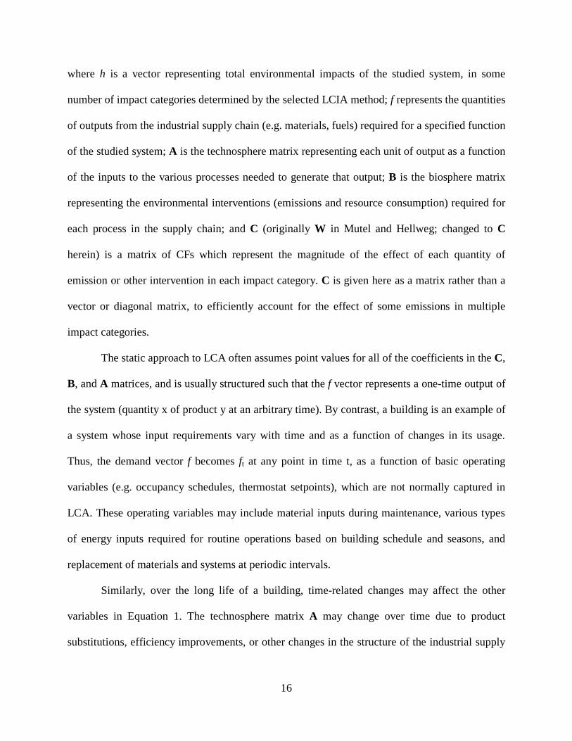
Given the potential for each term in Equation 1 to change over time, a simplified model
for DLCA is shown in Figure 1 and represented mathematically by the following:
Equation 2
ttt
te
ttt fh ×××= −∑ 1
0
ABC
where the t represents a point in time at which the values in the various terms are known, and t0
and te represent the beginning and ending time points of the analysis, usually the beginning and
end of the product or system life cycle. The t subscript does not imply that these terms are direct
mathematical functions of time; rather, they are functions of their underlying variables that can
be represented as a time series. Particularly, the matrix of CFs, Ct could encompass variations in
all the underlying variables (fate, exposure, and effect factors), which must be calculated for
each point in time by the physical models applicable to each category. Ct could also encompass
adjustments made to CFs for other reasons, such as proximity to the analysis time horizon, as in
Kendall (Kendall 2012). Separate types of changes to CFs could be explicitly documented by
constructing several separate C matrices (e.g. Ct, [fate] or Ct, [time horizon]) and combining these
matrices by scalar multiplication (Hadamard product) at the time of analysis.
18
Figure 1 - Conceptual diagram of DLCA framework
There are several considerations to this approach. First, this approach follows an
attributional, rather than consequential LCA structure (Ekvall and Weidema 2004). In
attributional LCA, the impact of an emission is considered to be the total impact of the product
system normalized to a functional unit,, whereas consequential LCA investigates the effects of
marginal choices. In the attributional formulation of the DLCA model, the aggregation is
performed at the time step level (variations at smaller scales are implicitly averaged). Thus, the
terms in eq. 2 are able to vary independently of each other. However, the use of dynamic
modeling of system interactions introduces the possibility of feedback loops in which changes
occurring in different parts of the system induce mutual changes in each other. The inclusion of
feedback loops between variables in Equation 2 (e.g. coefficient Ai,j relating process i to product
j as a function of fj, the quantity of product j required) would move the model partway toward a
consequential LCA structure (e.g. marginal effects on power or district heating generation from
adding a building to the utility grid). However, a fully consequential LCA requires a general
equilibrium economic model with many additional assumptions about changes in industrial

19
relationships based on additional or changed demand for goods and services. A fully
consequential LCA structure is sometimes used in large-scale policy analysis but may not be
appropriate for the study of individual buildings. For the current study, feedbacks are
hypothesized to be significant only within the systems captured by the building energy model
that produces the f vector. These feedbacks are briefly discussed in Section 2.4.1.
Another consideration is the issue of lag time in the supply chain, where lag time is
defined as the difference in timing of processes and emissions at multiple levels in the supply
chain (Levine et al. 2007). Some examples are the time difference between the production of a
building material and its installation at the construction site, or the time difference between fuel
extraction and combustion. For the simplified mathematical model in Equation 2, supply chain
functions must be assumed to occur simultaneously in order to invert the A matrix. A more
complete formulation would involve specifying the lag time for each supply-demand linkage,
which would require calculation using a tree structure rather than a matrix structure, as the
number of inputs at different time lags would multiply with each step back through the supply
chain. This approach could be implemented with an inventory or impact cutoff tolerance.
However, data limitations prevented the inclusion of lag times in this study as discussed further
in section 3.4.
A prototype DLCA model was constructed using Microsoft Excel and Visual Basic for
Applications (VBA). The model used Excel worksheets to store basic data such as process inputs
and outputs, emission factors and CFs, while VBA code was used to perform the matrix
calculations. The key difference between the prototype model and most standard LCA
applications was the use of time series tables to simulate dynamic variation in matrix coefficients
representing modeled relationships. With the time series enabled, any coefficient ci in a vector or

20
ci,j in a matrix can become ci,j,t, where i and j represent the coefficient’s position in the matrix in
question and t is the current model time step. The model explicitly considered four categories of
time series in the LCA calculation, corresponding with the four variables of Equation 2. These
categories are outlined in Table 1, along with illustrative examples. Any variable without a time
series available due to data limitations was assumed to have a constant value, as in a typical
static LCA calculation.
3.2.2 Case study
An existing institutional building – Benedum Hall at the University of Pittsburgh – was
selected as the case study for this project. Originally constructed in 1971 to house the
engineering program, the Benedum Hall complex includes a twelve-story tower housing
laboratories, offices and classrooms; two below-grade floors with additional office and
laboratory space, and a two-story auditorium. The two below-grade floors extend under the
footprints of both the tower and the auditorium, and support a first-floor level outdoor plaza. The
complex underwent a major renovation beginning in 2006, including the construction of a new
wing on the first, second and third floors; major upgrade of all mechanical systems; replacement
of all the windows and floor coverings; roof replacement including green roof spaces on both the
auditorium and a portion of the plaza; and numerous interior space renovations. The additional
wing and renovation of the 2nd floor of the tower were completed in November 2009; roof and
window replacement on the remaining structure and renovations of the below-grade floors,
ground floors and auditorium were completed by August 2010, and renovations of the 3rd-12th
floors of the tower are scheduled to be completed by the end of 2012. [UPDATE: 7th floor was
completed as of September 2012. Work continues on floor 8-12 as of this writing].

21
Since the original construction, steam for heating the building has been supplied by a
district heating system used by the University and several nearby institutions. Until June 2009,
steam was generated using a combination of coal-fired and natural gas-fired boilers at a single
plant; in June 2009, a second plant was added and the existing plant was converted to 100%
natural gas-fired boilers. Cooling was originally provided by a stand-alone chiller plant on the
building’s roof, which was replaced by a connection to a new district chilled water plant in 2002.
Table 1. Categories of dynamic life cycle assessment (DLCA) parameters for buildings, examples, and data sources
used in the case study.
Category [with parameter from Equation 2 in bracketsa]
Examples Data used in case study with associated time interval
Building Operations [ft]- initial construction activities; additions, renovations, or major component replacements; changes in usage patterns or energy consumption
Material required for initial construction; material required for replacement of components or reconfiguration of interior spaces; changes in energy consumption
-Benedum Hall original construction plans; 1971 (DRA 1965) -Benedum Hall utility usage (steam, electric, and water); 7/1992-12/2010
-Benedum Hall construction plans for renovation and addition; 2006-2010 (Edge 2007, 2008) -eQUEST model (projected); 2009-2045
Supply chain dynamics[At]- changes to upstream processes independent of building management decisions
Changes in fuel mix and efficiency of the electricity grid; changes in origin of natural gas and petroleum supplies; changes in regional waste treatment practices
-District heating plant fuel consumption and steam production; 1/2000-12/2010
-National annual and monthly electric power generation by fuel type; 1970-2008 (USDOE 2010b): (projected); 2009-2045 (USDOE 2010a)
Inventory dynamics [Bt]- changes in resource use or pollutant emissions by processes due to technology, regulation or other factors
Influence of environmental regulations on pollutant emissions; changes in efficiency of industrial processes
-National GHG emissions from electric power generation by fuel type and other major GHG sources; 1990-2008 (USEPA 2010) -National criteria air pollutant (CAP) and hazardous air pollutant (HAP) emissions; 1970-2008 (USEPA 2009, 2011b): (projected); 2009-2016 (USEPA 2011a)
Environmental system dynamics [Ct] – changes in background environmental systems affecting the fate, exposure and effects
Changes in system sensitivity due to background concentrations or distribution of populations; changes in ambient conditions affecting emission fates; consideration of an analysis time horizon
--Time adjusted (global) warming potentials (TAWPs); 2009-2045 (Kendall 2012) -Seasonal characterization factors for photochemical ozone; 2009-2045 (Shah and Ries 2008)
aParameter definitions: [ft]- vector of outputs from the industrial supply chain (e.g. materials, fuels); [At]- matrix representing each unit of output as a function of the inputs to the various processes needed to generate that output; [Bt]- matrix representing the environmental interventions (emissions and resource consumption) required for each
process; [Ct] – matrix of characterization factors representing the magnitude of the effect of each quantity of emission or other intervention in each impact category

22
3.2.3 Static and dynamic LCA comparisons
The DLCA model and a static LCA model were compared over two analysis time frames.
The first time frame consisted of the entire lifetime of the building and used a 1971 perspective;
while the second time frame consisted of the remaining life of the building using a 2009
perspective. We will refer to these as the “full lifetime” and “remaining lifetime” analyses
hereafter. The system boundary for both static and dynamic analyses included building materials
and operating fuels/electricity, as well as their respective upstream processes. The system
boundary of the DLCA model, including the extent of dynamic processes included, is shown in
Figure 2. Material transportation, on-site construction activities, routine maintenance and end-of-
life disposition were excluded from the study. Due to the complexity of modeling the entire
building, only major systems were selected from the initial construction, and a comparison was
made to two previous studies to assess the degree of completeness of the results (Junnila et al.
2006; Scheuer et al. 2003).
The full lifetime of Benedum Hall was assumed to be 75 years, consistent with its current
status (recently renovated at 40 years old) and one previous study of an institutional building
(Scheuer et al. 2003). It has been noted that arbitrary assumptions about building lifetime can
significantly affect LCA results (Aktas and Bilec 2012). The full lifetime DLCA encompassed
four distinct phases: 1) initial construction (1971); 2) initial operations (1971-2008); 3)
renovation activities (2006-2012); and 4) future operations (2009-2045). The renovation
activities were assumed to occur in 2009. Construction material quantities from the original
construction, renovation and addition were obtained from the construction drawings and
specifications for each project (DRA 1965; Edge 2007, 2008). The full lifetime static LCA
coupled the initial construction results with a projection of the initial year’s operations over the

23
75-year assumed building lifetime, and did not include the renovation/addition. The remaining
lifetime DLCA and static LCA included the renovation and future operations phases. The
remaining lifetime DLCA was used as the basis for the future scenario analysis (Section 2.5).
Figure 2 - System boundary and dynamic modeling
For this study, the DLCA model used a monthly time series for several reasons.
Historical values for the building’s utilities were available on a monthly basis, and fuel mixes for
the electricity grid (USDOE 2010) and heating plant were also available on a monthly basis
(Section 2.4.2). Annual aggregation of these values would potentially have masked variation in
the results due to the timing of variations in energy use and the fuel mix. Emissions factors were
typically annual values.

24
3.2.4 Data collection
Dynamic LCI - building-level data and modeling (ft) - Historical and future values for the
f vector were generated specifically for the case study building. Operating energy consumption
was taken from utility meter data for Benedum Hall. Data availability varied depending on the
individual variables; a summary is provided in Table 1 and a complete list is given in Table 14.
For years prior to data availability, the average of the first three available years was used. Future
energy consumption was estimated using the U.S. Department of Energy’s (USDOE) eQUEST
model (Hirsch 2010), adjusting model default parameters to reflect the specific conditions for
Benedum Hall. A qualitative comparison of the eQUEST model results and both the extensive
pre-renovation and limited post-renovation utility meter data was performed to verify the
model’s predictive capacity; results of this comparison are presented in Figure 24 and Figure 25.
Dynamic LCI - unit processes (At) - Temporally specific historical and projected future
unit processes for the A matrix were constructed from U.S. Energy Information Agency (EIA)
records and projections (USDOE 2010, 2011b) for the national electricity generation mix; and
meter data for the central campus steam plant (Table 14). Data sources for each process type are
provided in Table 1. Upstream processes without dynamic data available were referred to 1)
USLCI unit processes (NREL 2011), for energy and fuels; and 2) the ecoinvent v2.2 database
(ecoinvent 2010), for materials. Ecoinvent was chosen over USLCI for materials because some
material processes in the USLCI database do not explicitly link to upstream processes, but rather
aggregate emissions from all upstream processes into one list. Separation of upstream unit
processes was necessary to enable the DLCA model to function properly. However, because
ecoinvent consists of mainly European data and does not contain time series, several
modifications were made: 1) process electricity requirements from materials in ecoinvent were

25
referred back to the time series described above, and 2) other process energy (e.g. heat,
equipment fuel use) were referred to the USLCI energy unit processes. Thus, the material
processes used for the 1971 construction were the same as those used for the 2009
renovation/addition, with the exception of changing the fuel mix and emissions for the electricity
generation required by these processes.
Dynamic LCI - emissions factors (Bt) - Temporally specific emissions factors for the B
matrix were constructed from available industry and environmental data (USEPA 2009b, 2010,
2011b) and Allegheny County Health Department (ACHD) data for the central campus steam
plant (Kelly 2011). For example, emission factors for criteria air pollutants (CAPs) from electric
power generation were calculated by dividing U.S. Environmental Protection Agency (EPA)
historical emissions data (USEPA 2009b, 2011b)by the U.S. Energy Information Agency (EIA)
records of power generation by fuel type (USDOE 2011b). Data sources for each variable are
provided in Table 1; time series of emission factor results in each LCIA category are presented in
Figure 26. Where possible, these values were compared against the USLCI database (NREL
2010) for consistency within the time frames for which the USLCI database applies. Qualitative
results of this comparison are also presented in Figure 26.
Dynamic LCIA - characterization factors (Ct) - Temporally specific CFs are only
available in a few LCIA categories. Therefore, for the baseline full lifetime and remaining
lifetime DLCA calculations, static factors from the TRACI method were used (Bare et al. 2003).
Temporally specific CFs available in the literature include monthly CFs for photochemical ozone
in the U.S. (Shah and Ries 2009); annual global CFs for ozone depletion (Struijs et al. 2010),
decadal-scale CFs for acidification and eutrophication in Europe (Seppälä et al. 2006), time-
horizon adjusted CFs for acidification in Europe (Van Zelm et al. 2007), and time-horizon

26
adjusted CFs for global warming, e.g. (Kendall 2012). The European acidification and
eutrophication CFs are not adaptable to the U.S. due to the lack of a U.S.-based database of
ecosystem sensitivities (Norris 2003). The lack of any consistent set of temporally variable CFs
for the U.S. across multiple impact categories led to the decision not to include them in the
baseline analyses for this study. However, example calculations using two sets of dynamic CFs -
photochemical ozone from Shah and Ries (Shah and Ries 2009) and global warming (Kendall
2012) have been included in the future scenario analysis (Section 2.5). The compilation of a set
of temporally variable CFs across multiple impact categories and time scales for the U.S. is
planned as future work.
3.2.5 Future scenario analysis
A future scenario analysis was conducted to probe the sensitivity of the results to changes
in assumptions about future trends, building on the remaining lifetime DLCA calculation (2009-
2045). The individual and combined influence of end-use energy variations, fuel mixes, and
emissions controls was investigated by pairing different combinations of each variable in Eq. 1.
For ft, scenarios were generated using 10% increases and decreases in electricity consumption
and steam heat consumption separately. This range was anticipated to be within the capacity of
adjustments to existing set points and operating schedules, and thus allowed for some level of
uncertainty in occupant usage and behavior. For At, the EIA’s 47 projected cases from the
Annual Energy Outlook (AEO) were examined and the cases which resulted in the greatest
variation in generation mixes from the baseline were added to the analysis (USDOE 2010). For
Bt, a scenario without the EPA’s currently proposed regulations was examined, in which
emissions factors remained constant at 2009 levels. The scenario pairing no increase or decrease
27
in energy consumption with no new EPA rules was similar to the static LCA, except that even
the EIA’s baseline (Reference case) includes expected changes in the future generation mix and
is thus dynamic.
Finally, for Ct, calculations were constructed in the GWP category using time-adjusted
warming potentials (TAWPs) from Kendall 2012, and in the photochemical ozone category
using monthly factors for a typical year from Shah and Ries 2009. Shah and Ries developed CFs
at the midpoint level for nitrogen oxides (NOx) and volatile organic compounds (VOC) in terms
of ppb O3*km2*day/kg emission. To compare with the static TRACI CFs, which use a reference
unit of kg NOx eq., the Shah and Ries CFs were normalized by dividing the monthly values for
NOx and VOC by the annual average value for NOx from their own study.
3.3 RESULTS AND DISCUSSION
3.3.1 Static LCA validation
Total mass of the materials and embodied energy inputs of the static LCA for the original
construction were compared with two previous studies of commercial and/or institutional
buildings in the US (Junnila et al. 2006; Scheuer et al. 2003) to validate LCA inputs. Scheuer et
al. analyzed a 6-story combination academic and hotel building in Michigan, and Junnila et al.
analyzed a 5-story office building in the U.S. midwest. Results of the comparison are
summarized in Table 2. A complete comparison of LCI results is given in Table 15. Total
normalized mass of Benedum Hall was estimated to be 1,670 kg/m2 and total embodied energy
to be 5,080 MJ/ m2, compared to 2,000 kg/m2 and 6,250 MJ/m2 for Scheuer et al., and 1,290

28
kg/m2 and 11,900 MJ/m2 for Junnila et al. Total annual operating energy was 3,920 MJ/m2,
compared to 4,100 MJ/m2 for Scheuer et al. and 1,320 MJ/m2 for Junnila et al.
The results of this study agreed qualitatively with Scheuer et al. in most categories, and
with Junnila et al. in some categories. A significant degree of variation is expected even between
comparable buildings, due to differences in construction details, selection of system boundaries
and the use of different LCI databases. The material systems included in this study for Benedum
Hall represented 90% of the results of the Scheuer et al. study by mass, and 74% by embodied
energy.
Table 2 - Mass and energy inputs for static LCA model of the building materials and initial energy consumption.
Material and Energy Results
Case Study: Benedum Hall
Scheuer et al. (2003)
Junnila et al. (2006)
Mass/ area
(kg/m2)
Energy/ area
(MJ/m2)
Mass/ area
(kg/m2)
Energy/ area
(MJ/m2)
Mass/ area
(kg/m2)
Energy/ area
(MJ/m2) Total materials 1,670 5,080 2,000 6,250 1,360 11,920 Original construction materials
1,570 4,250 NG NG 1,290 7,060
Renovation/ addition materials
100 820 NG NG 70 4,860
Annual operating energy - total
- 3,920 - 4,100 - 1,360
Annual operating energy - electricity
- 3,340 - NG - 700
Annual operating energy - heat
- 580 - NG - 660
NA = Not applicable NG = Not given (results are presented graphically)
Embodied energy was calculated as total nonrenewable energy. Results from two other LCA studies of commercial
or institutional buildings in the US are presented for comparison and validation.
Mass results on a system-by-system basis were comparable to Scheuer et al. (more detail
provided in Table 15); the differences in embodied energy can be attributed primarily to 1) the

29
exclusion from this study of internal finish materials, such as carpet and ceiling tiles and 2) the
value for embodied energy for steel from the LCI databases used. Finish materials such as carpet
and ceiling tile have high embodied energy contents and frequent replacement intervals, and
account for a significant portion of the total embodied energy results in Scheuer et al. The
amounts of such materials in Benedum Hall are minor by comparison with most buildings and
were not considered in this study. Compared with Junnila et al, the lower embodied energy per
unit mass can also be attributed in part to the exclusion of interior finishes from this study, since
items such as structural steel and concrete had reasonably similar value for total embodied
energy per unit area of the building. However, Junnila et al. also used a hybrid process-based and
economic input-output (EIO) based LCA model, which may have contributed to the difference.
From comparison with both studies, future work on the dynamic LCA model should include
finish materials such as paint, carpet and tile for the sake of full compatibility with other studies
and to accommodate buildings with larger amounts of these materials than Benedum Hall.
3.3.2 DLCA and static LCA results for full lifetime analysis
The DLCA results were lower than static LCA results in most impact categories with the
exception of nonrenewable energy use (NREU; +12%), as shown in Figure 3. The factors
affecting the DLCA results in terms of eq. 2 were (1) the building’s end-use energy consumption
(included in ft), (2) the electrical generation fuel mix (included in At), (3) the steam generation
mix (also included in At), and (4) emissions factors for the national electrical grid (included in
Bt). The results showed reductions of more than half in the categories of acidification (-57%),
human health respiratory effects (-61%), photochemical ozone (-55%), eutrophication (-53%)

30
and carcinogens (-57%). Non-carcinogens and ecotoxicity were reduced by lesser amounts (-
27% and -9% respectively). Global warming potential (GWP) decreased by 2%.
Figure 3 - Comparison of results from static and DLCA models, using the TRACI method.
Results are normalized to the total static LCA results for each category. Static LCA results were calculated as the
total of the initial construction and projection of the initial year’s operating energy consumption for the 75-year life
of the building. DLCA results are classified into four categories: Original construction materials; Pre-renovation
operations (operating energy consumption through 2008); Renovation and addition materials; and Post-renovation
operations (operating energy consumption 2009 through end of lifetime).
The largest differences in the results were due to the lowering of emission factors for
CAPs from 1970 to the present, documented by EPA’s extensive historical estimation of CAP
trends and continuing projected reduction in the near future through 2015 due to the EPA’s

31
proposed Transport and Toxics Rules. Data for hazardous air pollutants (HAPs) also exist in
EPA’s historical estimates and future projections, though coverage dates are generally more
limited (1990-2008). No such national database for water pollution was found, though estimates
are noted in the literature (Bare 2011). Therefore, the water emissions estimated herein are
primarily static values from the ecoinvent and USLCI databases. Additionally, water pollution
related categories such as eutrophication and ecotoxicity may be under-represented because
wastewater from the building was not included in the study.
The three toxic pollutant LCIA categories (human health cancer, human health
noncancer, and ecotoxicity) are typically affected by both air and water emissions of hazardous
metals and organic compounds. However, air emissions of metals from coal combustion
dominated the results in the three toxics categories. In accordance with EPA modeling
documentation, combustion-related air emissions of metals were projected proportionately to
particulate matter <2.5 µm (PM2.5) and organic compounds were projected proportionately to
total VOCs (USEPA 2011a). Non-carcinogens and ecotoxicity were affected to a higher degree
than carcinogens by water emissions, and thus do not show as much reduction from historical
levels, due to the use of static data for water emissions. Material production processes for the
construction and renovation had a proportionately greater impact in the non-carcinogens and
ecotoxicity categories than the other categories; however, operating energy consumption still had
the greatest impact. For ozone depletion, all processes considered in this LCA are minor sources,
and thus neither the static nor dynamic results were considered to be significant.
Changes in emissions factors had the greatest influence on the LCIA results, but the
remaining variables in eq. 2 (ft, At) were also important, particularly in the GWP and NREU
categories. Figure 4 shows the DLCA results as cumulative time series in each LCIA category,

32
normalized to the cumulative totals in each category as of 2008. Impacts from construction and
renovation are represented at a single point in time; realistically, these impacts occur over the
span of several years. The time scale associated with these activities is shorter than that for
building operations, even when operations are classified into phases between major renovations.
Since the temporal changes incorporated into the current analysis are mainly gradual and on the
order of decades, the treatment of material- and construction-related emissions as pulses were not
expected to influence the overall results.
Electrical energy consumption increased gradually during the period of pre-renovation
meter data availability, growing 10% from 1993-1994 through 2007-2008. Steam consumption
remained essentially constant during this same period. The cause of the increased electrical usage
was not known, but it was assumed to be from increases in laboratory and office equipment
demand, including computers. If electrical energy consumption was due to increased use of the
overall building (e.g. extended hours, increased ventilation etc.), it would be expected to result in
an increase in steam use as well. For the renovated building, modeled energy consumption of
both types increased. An increase in overall building footprint, coupled with increased heating,
cooling and fan usage demands from increased space ventilation requirements were responsible
for the increased energy consumption.
In the GWP category, the increasing trend in energy consumption was offset by a
decreasing trend in greenhouse gas (GHG) emissions from the energy supply chain. While the
electrical generation mix continues to rely heavily on coal-fired power plants, GWP for the
electrical generation sector decreased 11% from 0.72 kg CO2 eq/kWh in 1970, to 0.64 kg CO2
eq/kWh in 2008. GWP of the district steam production decreased 39% from 2.3 to 1.4 kg CO2
eq/kg steam, following the switch from mixed coal- and gas-fired generation to 100% gas in June

33
2009. However, the modest decrease in GWP/kWh from electrical generation was offset by the
modest increase in electrical usage over the building’s lifetime to date, and the larger decrease in
GWP/kg steam was offset by the larger increase in projected steam usage following the
renovation as noted above. Because the heating fuel switch and renovations occurred at nearly
the same time, the slope of the NREU curve in Figure 4 is higher post-renovation than pre-
renovation, while the slope of the GWP curve in Figure 4 remains the same. Because natural gas
emits fewer CAPs and HAPs than coal, the heating fuel switch also affected the curves in Figure
4, combining with the reduced emissions factors from electric power generation to reduce the
slope of the future curves.

34
Figure 4 – Cumulative time series of DLCA results in TRACI impact categories and nonrenewable energy
use. Cumulative totals are normalized to year 2008 totals (prior to renovation).

35
3.3.3 DLCA and Static LCA results for remaining lifetime analysis
The DLCA results for the remaining lifetime analysis were lower than the static LCA
results in every impact category shown in Figure 5. As with the full lifetime analysis, the static
LCA used energy mixes and emission factors from the year of analysis (2009) projected through
the remaining lifetime. However in contrast with the full lifetime analysis, the building’s end use
energy consumption was the same for both static and dynamic analyses, since no actual energy
data were available yet. Reductions in impacts from largest to smallest were: acidification (-
17%), photochemical ozone (-16%), human health respiratory effects (-15%), eutrophication (-
14%), carcinogens (-5%), NREU (-4%), non-carcinogens (-3%), ecotoxicity (-3%), and GWP (-
2%). As with the full lifetime analysis, the largest decreases were caused by a reduction in
emissions factors following environmental regulations (the proposed EPA Transport and Toxics
rules). The reductions in global warming potential and nonrenewable energy use were due to
changes in the electrical fuel generation mix.
3.3.4 Future scenario analysis
The maximum variations from the baseline for the different DLCA scenarios are shown
as error bars on the DLCA results in Figure 5. These error bars represent the scenarios
contributing to the minimum and maximum impacts in each category. Other types of uncertainty
and variability (not shown) include parameter uncertainty (e.g. emissions factors) and spatial
variations. These uncertainties can be elicited by Monte Carlo analysis (e.g. Dale et al. 2013) and
could be shown as an additional set of error bars, applied to both the static and dynamic LCA
results. For the baseline energy use case, the minimum and maximum variability from the static

36
LCA due to combining variability in projected energy mixes and emissions factors were:
acidification (+39%/-18%), photochemical ozone (+36%/-15%), human health respiratory effects
(+35%/-22%), eutrophication (+32%/-20%), carcinogens (+20%/-34%), non-carcinogens
(+10%/-12%) and ecotoxicity (+9%/-9%). The minimum and maximum variability for categories
depending only on energy mixes were nonrenewable energy use (+7%/-15%) and global
warming potential (+10%/-17%).
Figure 6 shows selected time series for the global warming and photochemical ozone
impact categories, representing scenarios with different combinations of variation from the
baseline, for each term in eq. 2. The remaining series are presented in Figure 29. Of the
variations in the f vector, the 10%+/- electricity scenarios had greater influence than the 10% +/-
heat scenarios, due to 1) the larger overall energy use represented by electricity for this building,
and 2) the larger impact in most categories per unit energy of electricity, due to the use of coal as
a fuel. The variations in the f vector are a simple scaling of the baseline results, but are
qualitatively illustrative of uncertainty in building use, such as hours of operation, user behavior,
or HVAC system setpoints. They are also a point of reference in Figure 6 for the relative changes
in impact due to the scenarios representing variations of the A, B and C matrices.

37
Figure 5 - Comparison of predicted results for from static and DLCA models for the renovation and post-
renovation operations.
Error bars on the DLCA results indicate the minimum and maximum values associated with different scenarios from
the sensitivity analysis. For the GW and PO categories, the error bars include consideration of dynamic
characterization factors at the impact assessment step. Error bars for all other categories include only variation in the
life cycle inventory.

38
Figure 6 - Time series of DLCA results for the sensitivity analysis, shown as cumulative percent deviations
from the baseline scenario for the global warming potential and photochemical smog categories.
Time series plots of the deviations from baseline for the remaining TRACI impact categories are presented
in Figure 29.
Of the 47 electricity grid mix scenarios drawn from the EIA AEO (represented in the A
matrix), the greatest decrease in impact in most categories was the “GHG price economywide”
scenario, representing a future in which coal use drops steeply due its greater CO2 emissions than
other fuels. The AEO scenario with the greatest increase in impacts was the “low shale resource”

39
scenario, in which estimated unproven resources (EURs) are assumed to be half those in the
Reference case. The low availability of shale gas in this scenario leads to a reduced use of gas
and a corresponding increase in coal for electric power generation.
For any combination of f and A scenarios, eliminating the introduction of the new EPA
regulations (represented in the B matrix) showed increased impact in most categories associated
with CAPs (and some HAPs, such as metals from coal-fired power plants) compared to the
baseline DLCA case. Scenarios eliminating the new EPA regulations combined with low gas
resources - and hence increased coal use for power generation without significant new emission
controls - showed increased impacts in these categories compared even to the static LCA.
The effect of including dynamic CFs is shown in the odd-numbered curves in Figure 6,
and is reflected in the error bars in the global warming and photochemical ozone categories in
Figure 5. In both cases, the addition of dynamic CFs reduced the total impacts compared to static
CFs, though for different reasons. For global warming potential, the dynamic CFs, or TAWPs,
reduced the cumulative impacts for any combination of other variables by approximately 13% at
the year 2045. This reduction represents the application of a fixed 100-year time horizon for
integrating radiative forcing of GHGs, applied over the 36-year lifetime of the building. For
example, CO2 emissions in 2045 treated in this manner have a TAWP of 0.71, instead of 1. For
more information on TAWPs, see Kendall (2012). Although TAWPs for different GHGs vary
differently with time, CO2 was by far the dominant GHG in this analysis. Since the TAWP is
calculated on an annual basis, any process with a total lag time of less than 1 year is accurately
represented, which should capture the bulk of energy extraction and supply processes.
For photochemical ozone, the inclusion of dynamic CFs reduced the individual scenarios
resulting from the combination of the other variables by 26% to 50%. The reduction was lowest

40
for low emissions scenarios (e.g. Scenario 16 in Figure 6; 90% electricity with AEO GHG price
and new EPA rules) and highest for high emissions scenarios (e.g. Scenario 36; 110% electricity
with AEO low shale resources and no new EPA rules). The overall reductions are explained by
the fact that higher emissions of ozone precursors - mainly NOx in this case - occurred during
winter months, when the dynamic CFs are lowest. This was due to 1) overall increased demand
for energy in the winter, due to heating needs and 2) relatively constant year-round electrical
demand, but with a higher percentage of coal-fired power generation in winter months. Since the
photochemical ozone CFs vary on a scale of months, it is possible that including lag times could
affect this calculation. However, uncertainty in the supply chain required assuming an annual
average CF for all upstream processes, while using the monthly CFs for combustion. This
formulation implicitly resulted in a variable lag time of up to 1 year between upstream processes
and combustion.
3.3.5 Limitations
Additional dynamic CFs - CF variations were not considered in most categories because
no applicable source of temporally CFs was found in the literature. The lack of characterization
methods incorporating both short-term and long-term temporal variability is a shortcoming of
current LCA practice, and could be remedied by additional LCIA method development.
Temporally variable CFs need to take into account changes in background chemical
concentrations, environmental systems and the distributions of exposed populations, as well as
time horizon relevance. The examples used in this study represent one instance of a time horizon
related CF (TAWP) and one instance of a physical system variation (photochemical ozone). In
41
the case of the latter, additional investigation into the combination of daily, seasonal and long-
term factors is needed (Reap et al. 2008).
Data availability - Dynamic variation in industrial processes and emission factors is
hampered by a lack of available data. In this case study, unit energy use for industrial processes
and emissions factors from fuel use other than in electrical power plants, were not able to be
modeled dynamically. This resulted in lower energy use and emissions associated with building
material production for the initial construction. However, in LCIA categories that were highly
influenced by energy use, these contributions were small relative to the impacts of operating
energy. With respect to emissions factors, it is noted that continued increases in data quality are
expected to provide additional accuracy in results. Efforts to track and control toxic pollutants
have historically lagged behind CAPs, and thus there is greater uncertainty in the temporal trends
in toxic-related impact categories. With respect to lag times, the inclusion of supply chain lag
times as an additional variable in LCI databases is critical for the accurate application of
temporally varying CFs. However, the uncertainty related to upstream production functions may
require annual averaging of most processes except those occurring in the building itself, which
can be known with some detail, or those which are predictable based on system characteristics,
such as energy and fuel supplies.
Spatial variability - Significant spatial uncertainty exists in LCA. The definition proposed
herein for DLCA includes consideration of spatial variability, though it has not been directly
addressed yet in this analysis. Noting that the term dynamic usually connotes temporal changes,
it should be considered that spatial patterns of industrial activity and environmental impacts
change over time; the NEI and other databases provide explicit spatial detail related to emissions,
and LCIA methods with spatially explicit CFs are available. For North America, both TRACI

42
and Impact models have some spatial resolution, though additional detail is needed in most
categories. Related to spatial variation, it has been noted that there is extensive regional variation
in the electrical generation mix. The national generation mix has been used herein, but regional
or even sub-state-level mixes have been used in some studies. However, it has been shown that
power trading between regions tends to drive the mix toward a national average (Weber et al.
2010); thus, the use of non-spatially explicit factors may be warranted in this case. More so than
for electricity, the concentration of major producers in some industries (e.g. petroleum refineries,
mining) in specific regions with CFs different from the national average may lead to a case for
regionalization of LCA results even when the exact supply chain is uncertain.
Uncertainty of future scenarios - The outlook of this chapter comprises both historical
temporal variations and predicted future variations. However, it is likely that the primary use for
LCA of buildings will continue to be predictive. Uncertainty in future scenarios depends on both
building-level variables (e.g. occupancy levels, renovations) and external variables such as
emissions controls and environmental background conditions. Since Benedum Hall was recently
renovated, projection of past building-level trends into the future was limited to assuming as-is
operations of the building and district heating plants (since the building recently underwent a full
renovation), with variation in energy usage of +/-10% to accommodate occupant behavior.
However, exact knowledge of future occupant needs or renovation schedules will not usually be
available to the LCA practitioner, even with DLCA modeling. There are also predictive
assumptions built into the models used by EIA and EPA to forecast future energy mixes and
emissions. Though uncertainty in prediction cannot be fully avoided, considering multiple future
scenarios can illuminate possible environmental tradeoffs; for example, the often-cited tradeoff
between embodied energy in construction materials and use-phase operating energy is changed

43
somewhat when a DLCA model with varying energy supply background conditions is used.
Alternatively, a conditional probability approach could be used - explicitly accounting for the
choice of externally imposed scenarios to generate a scenario-independent DLCA result which
would include the other types of uncertainty (e.g. spatial, parameter) while still eliciting expected
changes from a static LCA over time (e.g. building systems performance).
3.4 CONCLUSION
This chapter explicitly uses dynamic LCA (DLCA) and illustrates the potential
importance of the method using a simplified case study of an institutional building. The results
show that the environmental impacts of the building over its lifetime vary significantly from
what would be predicted if temporal changes were not taken into account. Particularly, the
results indicate the importance of changes in building usage, energy sources and environmental
regulations in calculating the overall environmental impacts of the building. Given that temporal
changes are rarely accounted for in LCA practice, it seems clear that LCA could be improved by
incorporating a more dynamic focus. Previous whole-building LCAs have demonstrated the
relative importance of the operations phase in most impact categories, compared to the materials,
construction and end-of-life phases. The DLCA results suggest an additional conclusion; that in
some cases, changes in building usage, or changes in external conditions such as energy mixes or
environmental regulations during a building’s lifetime, can influence the LCA results to a greater
degree than the material and construction phases. Correspondingly, adapting LCA to a more
dynamic approach as demonstrated herein seems likely to increase the usefulness of the method
in assessing the performance of buildings and other complex systems in the built environment.

44
Future research needs include characterization of uncertainty related to building systems
modeling (e.g. future occupant needs and maintenance/renovation schedules); additional
exploration of the interactions with dynamic, temporally evolving (and themselves uncertain)
LCI and LCIA background variables, and development of additional dynamic CFs and dynamic
parameters for LCI databases.
Establishing a DLCA framework for whole buildings was considered to be an essential
prerequisite for incorporating indoor environmental quality (IEQ) effects into whole-building
LCA. The factors affecting IEQ impacts, particularly occupancy and operational schedules, are
subject to significant changes on daily and seasonal bases, as well as over the long term. The
following chapters deal with the incorporation of IEQ into the DLCA model and comparison of
internal to external effects.

45
4.0 INTEGRATING INDOOR ENVIRONMENTAL QUALITY INTO THE DLCA
FRAMEWORK FOR WHOLE BUILDINGS
The following chapter contains material reproduced from an article published in the journal
Building and Environment with the citation:
Collinge, W.O., A.E. Landis, A.K. Jones, L.A. Schaefer and M.M. Bilec (2013), “Indoor
Environmental Quality in a Dynamic Life Cycle Assessment Framework for Whole Buildings:
Focus on Human Health Chemical Impacts.” Building and Environment 62 pp. 182-190.
The article appears as published per the copyright agreement with Elsevier, publisher of
Building and Environment.
Portions of the Supporting Information submitted with Building and Environment appear
in this chapter and Chapter 5, and the remaining portions appear in Appendix B.
4.1 INTRODUCTION
The aim of this chapter is to outline a framework for incorporating IEQ into whole-
building LCA. Methods for empirically quantifying IEQ impacts generally fall into two types:
single variable relationships between building-related parameters and measured occupant health

46
or performance outcomes (Fisk and Mirer 2009; Heschong et al. 2002a; Mendell and Mirer
2009; Milton 2000; Seppänen et al. 2006c; Sahakian et al. 2009; Mendell 2003) and multivariate
indices with single-value or reduced-parameter predictors of occupant outcomes (Mendell 2003;
Sekhar et al. 2003; Sofuoglu and Moschandreas 2003; Wong et al. 2007).
Recent research integrating IEQ in LCA has focused on incorporating indoor chemical
pollutant intake into the existing human health toxicity life cycle impact assessment (LCIA)
categories (Demou et al. 2009; Hellweg et al. 2009; Humbert et al. 2011; Wenger et al. 2012). In
these approaches, the impacts of indoor pollutant emissions are estimated based on emission
rates from indoor materials or processes and building-level variables, such as ventilation and
occupancy rates. A benefit of these approaches is integration within existing conventional LCIA
categories. However, when extending the approach to consider whole-building IEQ features,
additional factors need to be included. These factors can be grouped into three categories: 1)
indoor intake of outdoor pollution due to a building’s location and ventilation characteristics, 2)
indoor generation of biological/biochemical contaminants, and 3) non-IAQ related influences on
occupants’ health and productivity (e.g. eye strain and mood impacts due to poor lighting
quality). Though the latter two factors may extend the boundaries of conventional LCA practice,
there is precedent for inclusion of similar effects in the LCA literature; e.g. noise, workplace
accidents (Cucurachi et al. 2012; Pettersen and Hertwich 2008). In the case of whole buildings
and other built environment systems, the case for including these system-dependent impacts is
made stronger by the function of the system under study (e.g. housing or transporting human
beings).
The overarching goal of this research project is to develop a dynamic LCA (DLCA) tool
for building analysis that incorporates metrics of relevance to building design. In Chapter 3, a

47
working definition of DLCA was proposed as “an approach to LCA which explicitly
incorporates dynamic process modeling in the context of temporal and spatial variations in the
surrounding industrial and environmental systems”, and its application was evaluated with a
simplified case study. The research questions addressed in the next two chapters are: “How do
we incorporate IEQ into LCA, and how significantly does IEQ affect conventional LCA
results?” To answer these questions, we developed a framework for including IEQ impacts in
whole-building LCA, separating chemical-specific impacts that align with traditional LCIA
categories from non chemical-specific impacts, and identifying potential gaps or overlaps.
Chapter 4 outlines the complete framework, and Chapter 5 applies the framework to a case study
of an existing LEED Gold academic building. We then compare these internal impacts to the
external impacts resulting from the DLCA model applied to the building’s energy use.
4.2 METHODS
4.2.1 General framework for Indoor Environmental Quality + Dynamic Life Cycle
Assessment (IEQ+DLCA)
The indoor environmental quality + dynamic life cycle assessment (IEQ+DLCA)
framework developed herein is illustrated in Figure 7. Beginning at the top of the figure, the first
distinction is between internal and external building impacts, which is a crucial element of the
framework. Internal impacts are defined as those occurring within the study building, whereas
external impacts are those occurring outside of the study building.

48
Figure 7 - IEQ+DLCA framework.
External LCA impact categories are shown on the left; internal impact categories are shown on the right.
For external impacts, shown on the left side of Figure 7, the IEQ+DLCA framework
builds on the dynamic LCA (DLCA) model developed in the previous chapter (Collinge et al.
2012a). A dynamic approach, considering the time variation in building-related measurements,
can reduce the uncertainty introduced by static estimates of building usage, as well as accounting
for variation in industrial and environmental systems. Inputs to the DLCA model are typical for
LCA - quantities of energy or materials required for building operations and maintenance - but
are input as time series to maintain correspondence with dynamic unit processes and emissions
factors. The DLCA model contains a standard set of impact assessment categories based on
TRACI 2.0 (Bare 2011), with optional dynamic characterization factors (CFs) limited to those
few categories for which values are available in the literature. Dynamic CFs are not currently
Toxicology-based: same units, directly comparable Empirically-based parametric relationships
IEQ+DLCA Framework
Internal impactsExternal impacts
Traditional LCIA human health
categories
Traditional LCIA categories outside
human health
Human health -chemical
• Cancer toxicity• Internal• External
• Noncancer toxicity• Internal• External
• Respiratory effects (particulates)
• Internal• External
Based on TRACI 2/ USE-Tox
Productivity and performance
Human health -nonchemical
• Global warming
• Acidification
• Eutrophication
• Ozone depletion
• Photochemical ozone
• Ecotoxicity
Based on TRACI 2
• Sick building syndrome symptoms (SBS)
• Allergies and asthma
• Building-related illnesses
• Other illnesses (e.g. stress, mood disorders)
• Sick leave,• At-work
productivity
Based on Fisk et al 2011
Legend
Potentially overlapping categories
Currently included Currently excluded
Category currently excluded due to lack of literature data
49
available for human health categories. TRACI 2.0 employs CFs from the UseTox model for
cancer and noncancer toxicity (Rosenbaum 2008b; Rosenbaum et al. 2011), and its own CFs for
respiratory effects, all of which are static values. If dynamic CFs for these categories are
developed in the future (e.g. seasonal and spatial variation in fate and exposure factors), these
could be incorporated into the DLCA model. With respect to human health, external impacts
could include impacts inside other buildings, such as occupational exposures related to industrial
processes in the supply chain. However, most LCIA methods do not yet explicitly consider such
impacts, though research is being undertaken toward this goal (Demou et al. 2009; Hellweg et al.
2009; Humbert et al. 2011); thus, their inclusion is not examined here.
Internal impacts are limited to human health impacts, since the remaining categories in
conventional LCA accrue to species or environmental systems (e.g. global climate). As defined
herein, internal impacts - shown on the right side of Figure 7 - affect users or occupants of the
building, during the time they are inside the building. In the external categories, human health
impacts accrue to either the global or continental population as specified in the underlying Use-
Tox LCIA model (Rosenbaum 2008b). Since the internal impacts are specific to the population
of occupants of the subject building, there will be some finite but small overlap between these
populations. Herein we assume that this overlap is negligible, and its potential effects are
discussed in the next section.
Internal impacts are further separated into three types; 1) human health chemical impacts,
2) human health nonchemical impacts, and 3) performance or productivity impacts. For all three
categories, a specific set of dynamic building data is required (Figure 8), including indoor and
outdoor air temperatures (ambient and supply air); ventilation and recirculation airflows and
filtration or other treatments; humidity; lighting; and noise levels. Evaluation of chemical

50
impacts also requires indoor pollutant emissions, or indoor and outdoor pollutant concentrations.
For all types of internal impacts, the dynamic estimation of building occupancy levels is critical
to calculate temporally specific exposures. Chemical impacts are disaggregated into 3 categories;
respiratory effects, cancer toxicity, and noncancer toxicity. These categories are the same in
terms of dose-response or effect factors as their external (conventional) counterparts (Figure 8),
but with different methods used to calculate exposure, described in more detail in section 4.2.2.
Figure 8 - Flowchart showing inputs, calculation steps and outputs for internal human health-chemical impact
categories and external LCA impact categories.
LegendData flow Data or steps not included in this study Data from reference sourcesData which can be measured or calculated from other variables
Internal human health chemical
impacts
Productivity and performance
Human health -nonchemical
Dynamic impact assessment –
external impactsDynamic inventory
analysis
Unit processes
Emissions factors
Exposure factors
Intake fractions(exposure + fate)
Empirical parametric
relationships
Dynamic building occupancy data
Energy use
Dynamic pollutant dataInternal emissions
OR Indoor concentrations
Outdoor concentrations
Dynamic operating dataAirflows
Temperature HumidityLighting
AcousticsOutdoor climate
Dynamic exposure estimates
Water use
Material use
Dynamic impact assessment –
internal impacts
External human health chemical
impacts
External other impacts
Effect factors
Fate factors

51
4.2.2 Whole building exposure approach for chemical impacts
The general approach to LCIA consists of multiplying emissions collected in the LCI by
CFs, which relate emissions to health impacts through the use of fate, exposure and effect
modeling (Rosenbaum et al. 2011). This approach is incorporated in the IEQ+DLCA framework
for internal and external chemical impacts, as shown in Figure 8. The CFs can be broken down
into a fate factor (FF), an exposure factor (XF), and an effect factor (EF). The expression FF x
XF is often defined as the intake fraction (iF) - the total fraction of an emission inhaled or
ingested through multiple exposure pathways (Bennett et al. 2002). An advantage of the iF
approach is that it combines temporally and spatially explicit environmental (fate and exposure)
modeling into a single parameter, while maintaining the use of separate EFs derived from
toxicological studies.
However, emissions factors for indoor materials and processes during a building’s use
phase are often lacking in LCA (Verbeeck and Hens 2010a, b). Conditions under which
contaminants are emitted from building materials or indoor processes may be highly site-
specific, and may depend on reactions with outdoor pollution, sunlight, humidity or other factors.
Herein, the single-compartment box model developed by Hellweg et al. (Hellweg et al. 2009) is
modified to use measured concentrations as opposed to emissions factors, and expanded to
permit the use of a multi-compartment model appropriate for a standard modern office building
with separate ducted supply and return air systems. It is possible to consider such a building as a
set of well-mixed compartments where the infiltration, exfiltration and inter-compartment air
exchange rates are small in comparison to the mechanical air circulation rate (ASHRAE 2009).
Typically, interior air is circulated to a central air handler through the return ductwork, where
some fraction of the return air is exhausted to the outdoors and the remainder is combined with

52
fresh outdoor air. The mixed air is filtered or otherwise treated to remove contaminants and then
supplied to the interior space, with the supply and return air to each compartment approximately
balanced to avoid inter-compartment mixing (ASHRAE 2009). Figure 9 shows a schematic of
this type of system.
Figure 9 - Schematic of multicompartment IAQ model.
Variables are the following: Q = airflows (m3/min), C = concentrations (ppm or µg/m3), G = emissions rate (g/min),
R = removal rate (g/min), N = persons, subscript x denotes a specific contaminant, and the subscript s, r, m, ex and
oa denote supply air, return air, mixed air, exhaust air and outside air, respectively.
Beginning with the single-compartment box model, the steady-state intake fraction for
indoor emissions is written by Hellweg et al. (Hellweg et al. 2009):

53
Equation 3
NkV
IRNQIRIRN
GQGIRN
GCiF
exx
x
x
x
×==×
∂∂
=×∂∂
=)/(
where Cx is the concentration of airborne contaminant x (kg/m3) in the compartment, Gx is the
emission of contaminant x in the compartment (kg/day), N is the number of persons exposed, IR
is the average inhalation rate (m3/person*day), Q is the ventilation rate (m3/day), V is the volume
of the compartment (m3), and kex is the air exchange rate (day-1). This terminology is extended to
express the total impact hx for contaminant x in a single LCIA category by Equation 4:
Equation 4
EFNkV
IRGEFiFGhex
xxx ××
×=××=
If the variables N, IR and EF in Equation 4 are known, and can be supplemented with
measured concentrations Cx, then by the definitions in Equation 3, Equation 4 can be rewritten:
Equation 5
xxx EFNIRCh ×××=
One potential advantage of a measured-concentration approach is its ability to
incorporate indoor exposure from outdoor ambient pollution. Indoor exposure may occur
because of the intake of outdoor contamination into the building, such as combustion emissions
from nearby roadway traffic. This contamination depends upon the building’s location and is the
result of many processes both related and unrelated to the life cycle of the building. However, for
whole-building LCA we may wish to estimate the building-specific exposure due to intake of
outdoor emissions, regardless of the source. This exposure, while not attributable to individual

54
building materials, can be considered part of the LCA of the building for the purpose of
comparison to a baseline, or the evaluation of alternative building designs.
For a multi-compartment model, a modified version of Equation 5 can be written:
Equation 6
∑ ×××=ti
xtitixx EFNIRCh,
,,,
where the subscript i refers to individual compartments in the building, and the subscript t refers
to the time interval at which the concentrations and occupancy are measured. In the case of
internal building emissions vented to the outdoor environment, additional populations may be
exposed. The multi-compartment model can be extended to this case by considering an
additional compartment to represent the local environment, with an effective mixing volume
based on local meteorological characteristics. In the multi-compartment model, using indoor
emissions factors instead of measured concentration data requires additional computation, since
in the case of air recirculation, the concentration in every compartment is related to emissions in
each other compartment.
Figure 9 shows the case of a typical office building with separate ducted supply and
return air systems. We consider the building as a set of well-mixed compartments where the
inter-compartment air exchange rate is small in comparison to the mechanical air circulation rate.
Typically, interior air is brought back to a central air handler through the return ductwork, where
some fraction of it is exhausted to the outdoors and the remainder is combined with fresh outdoor
air. The mixed air is filtered to remove contaminants and then supplied to the interior space, with
the supply and return air to each compartment approximately balanced to maintain similar space
pressures, thereby avoiding inter-compartment mixing.

55
Assuming negligible pressure differences throughout, so that mass flows can be
considered proportional to measured volumetric flows, we can write a mass balance for the
whole building:
Equation 7
exrcoarcrs QQQQQQ +=+==
where Qs is the supply air flow from the air handler, Qr is the return air flow from all
compartments, Qrc is the recirculated air flow, Qoa is the outside air intake, and Qex is the exhaust
air flow to the outdoors. With balanced compartments, the supply and return flow to each
compartment i will be Qi.
The concentration of any given contaminant x in compartment i is Cx,i, and is affected by
the concentrations in the recirculated air (Cr) and the outdoor air (Coa), as well as the indoor
emissions Gx,i in compartment i, removal Rx,i in compartment i due to settling, adsorption,
chemical reaction or other means. We can perform a mass-balance for contaminant x in
compartment i as the following:
Equation 8
ixisxiixixiixix CQCQRGV
dtdC
dtdm
,,,,,,
−+−==
where mx,i is the mass of contaminant x in compartment i and Vi is the mixed volume of the
compartment. We assume each compartment is well-mixed, such that the concentration in the
exhaust air stream is equal to the concentration in the compartment Cx,i. The concentration in the
return air at the air handler will be the weighted average by flow of the concentrations in the
individual compartments:

56
Equation 9
r
iixi
rxQ
CQC
∑=
,
,
The concentration of contaminant in the supply air will be influenced by the building-
wide ratio of recirculated air to outside air, as well as filtration or other removal at the air handler
or in the ductwork:
Equation 10
xs
oaoaxrcrxsx FF
QQCQCC ,,
,+
=
where the term FFx represents the fraction of contaminant retained in the supply airstream after
filtration or other removal.
Combining Equation 8 through Equation 10, we can write the mass balance for
compartment i:
Equation 11
−+
+−=
∑
ixxs
oaoaxrcr
iixi
iixixiix CFF
Q
QCQQ
CQ
QRGVdt
dC,
,
,
,,,
Solution in the case of known concentrations and flows- For steady-state conditions,
dC/dt = 0 and if the Q and C terms are known, Equation 12 can be solved straightforwardly to
obtain G - R. For a time-varying condition, if the concentrations Cx,i and Qi are measured at some
time interval Δt, an approximate solution for the quantity Gx,i - Rx,i representing net emissions of
contaminant x in compartment i can be written as the following:

57
Equation 12
−+
+−=− ∆−∆−
∑
ttixxts
toatoaxrctr
itixti
titixtixittixtix CFFQ
QCQQ
CQ
QRGVCC ,,,
,,,,
,,,
,,,,,,,,, )(
In some cases, it may be practical to ignore compartmental removal rates Rx,i and
consider the emissions equal to the net emissions. This is the case in the example of measuring
occupancy levels from CO2 concentrations and airflows, discussed below.
Intake fraction solution in the case of known emission rates- While Equation 12 can be
solved separately for (G - R) for each compartment given values for the C and Q terms, it is not
possible to solve it for C given G, R and Q. For steady state conditions, expanding the
summation term in Equation 11, substituting Qr = Qs and rearranging yields:
Equation 13
0... ,,,1,1,, =−
+++− + ixix
s
ioaoaxnxn
s
rcx
s
rcixix CQFF
QQQCCQ
QQCQ
QQRG
Writing Equation 13 for each compartment i = 1,2,3…n results in a system of n linear
equations and n unknown concentrations, assuming net generation and removal rates are known
along with compartment sizes, airflows and the outdoor concentration Cx,oa. The system can be
solved simultaneously to yield concentrations. Equation 13 can be rewritten for the whole
building in matrix notation:
Equation 14
0Acrg =−−
where g, r, and c are nx1 vectors representing the emissions, removal and concentration in the n
compartments and A is an nxn matrix of the coefficients applied to the concentration terms,

58
calculated from the remaining flow and ratio terms in Equation 13. If in-compartment removal
rates area small, r can be neglected, and solving for the vector of concentrations c yields:
Equation 15
gAc 1−=
To obtain the whole-building intake fraction for emissions in any compartment we first
must calculate the change in the concentration vector as a function of the change in Gx,i:
Equation 16
ixix Gg
Gc
,, ∂∂
=∂∂ −1A
All terms in the right hand side of Equation 16 are zero (since the emission rates in the
different compartments are independent) except for the term related to Gx,i (since ∂Gx,i/ ∂Gx,i =
1); thus:
Equation 17
1A −=∂∂
iixG
c,
where Ai
-1 represents row i of the A-1 inverse matrix.
The intake fraction associated with an emission in compartment i is calculated by combining
Equations 3 and 17, where n is now a vector of the number of persons in each compartment:
Equation 18
IRIRG
ciF iix
×=×∂∂
= − nAn 1
,
Outdoor and indoor exposure and overlaps - Impacts of indoor emissions vented to the
outdoors could be represented by the addition of an outdoor compartment with mixing
characteristics established from local meteorology, along with local population data.

59
There will be some finite overlap of the population exposed to indoor pollution and the
population exposed to outdoor pollution. We can consider a building located in a default
continental or urban box as outlined by the Use-Tox model (Hellweg et al. 2009). The external
intake is thus life cycle emissions x per capita intake fraction x external(urban or continental)
population. Concurrently, the internal intake considering exposure to outdoor pollution, is indoor
concentration x per capita indoor intake x internal population (occupancy). The key to the
overlap being small is that internal population must be small compared to external population,
and the life cycle emissions within the continental or urban box volume must be small compared
to the ambient pollution levels. The internal to external population ratio is further reduced by the
ratio of the average amount of time the occupants spend indoors versus outdoors. In the case of a
geographically isolated building with high on-site emissions, the overlap would be substantial. In
the case of a medium-sized building in a large urban area, with a spatially diverse supply chain
(e.g. the electrical grid) the overlap would be small, which is the case represented in the current
chapter.
4.2.2.1 Estimating occupancy using CO2 concentrations
A measurement or estimate of occupancy is necessary to calculate intake fractions or
total intakes by Equation 3 and Equation 5. Occupancy can be calculated using measured CO2
concentrations, HVAC system airflows and known values of human respiratory CO2 output, as
long as no other significant sources or sinks of CO2 exist within the compartment (e.g.
combustion or passive ventilation). Equation 12 can be used to determine CO2 emissions in each
compartment given RCO2 = 0 (no interior removal) and FFCO2 = 1 (no filtration). Rewritten
explicitly for CO2, Equation 12 becomes:

60
Equation 19
−+
+=− ∆−∆−
∑
ttiCOts
toatoaCOrctr
itiCOti
titiCOittiCOtiCO CQ
QCQQ
CQ
QGVCC ,,,
,,,,
,,,
,,,,,,, 2
2
2
222 )(
The rate of CO2 production (rCO2)due to human respiration under office building-type
conditions is approximately 0.026 kg CO2/hr, with a low estimate of 0.018 kg/hr and a high
estimate of 0.036 kg/hr (Emmerich and Persily 1997).
Equation 19 was solved for each 20-minute time step corresponding to the OptiNet
sampling rate. Due to the scope of the data collection, several additional assumptions were made:
• The air handler serving the 2nd and 3rd floors of the MCSI addition also feeds other areas of
the building, some of which are monitored for CO2 concentration and some of which are not.
The concentration of CO2 in the return air at the air handler (corresponding to the summation
term in Equation 19 divided by Qr) was not directly measured, but was assumed to be the
same as calculated applying the same formula to the sample of rooms where the in-room
concentrations were monitored. In other words, the average concentration in non-monitored
areas was assumed to be the same as the average concentration in monitored areas, for the
same time step.
• Outside air and recirculated airflows were not directly measured, but were estimated based
on the total supply airflow and the economizer percent open (EO%) at the air handler, which
varied from its preset minimum of 20% outside air to 100% outside air under favorable
outside temperatures. The concentration of CO2 (CCO2,s) in the supply air was calculated by:
Equation 20
%,%,, )1( EOQCEOQCC soaxsrxsx ×+−×=
After solving Equation 19 for GCO2,i,t, the number of persons in each compartment (Ni,t)
was calculated by Equation 21:

61
Equation 21
2
2 ,,,CO
tiCO
rGtNi =
4.2.2.2 VOC Speciation and inhalation toxicity
The USE-Tox model, developed for the UNEP-SETAC Life Cycle Initiative, contains
estimates of human toxicity in cancer and noncancer effects categories (Rosenbaum 2008a).
USE-Tox calculates intake fractions (iF) and effect factors (EF) for use in Eq. 2. In the indoor
model, iFs are calculated from primary data, but require the use of independent EFs to aggregate
the effects from multiple substances into these categories. The same substance-specific EFs are
used in Eq. 3 to calculate impacts in the multicompartment model with known concentrations
and occupancy. The USE-Tox model documentation provides a list of already-calculated EFs for
many common organic (including VOCs) and inorganic substances, and is available at
www.usetox.org. A list of the USE-Tox EFs for all VOCs in this study is given in Table 18.
To estimate the overall inhalation toxicity of an air volume, the individual VOC mass
concentrations were multiplied against their EF (cases/mass inhaled) to give a result in terms of
cases/volume of air inhaled, which can be considered an ambient air-specific EF:
Equation 22
∑ ×=x
xxair EFCMEF
where EFair is the ambient air-specific EF, CMx is the mass/volume concentration of contaminant
x, and EFx is the effect factor for contaminant x in either the carcinogen or non-carcinogen
category.
The 10.6 electron-volt (eV) photoionization detector used in the OptiNet system
generates a total VOC (TVOC) reading in equivalent ppm of isobutylene. For individual species,

62
conversion factors may be applied to estimate the equivalent TVOC reading generated by a
known concentration. PID conversion factors are listed in Table 18.
The equivalent TVOC measurement in ppm isobutylene for a given mixture of VOCs is
given by Equation 23:
Equation 23
∑ ×=x
xxTVOC PIDCC
where Cx is the concentration in ppm of each VOC species x and PIDx is the corresponding PID
equivalency factor. If concentrations are given in mass units, e.g. μg/m3, the conversion
becomes :
Equation 24
∑ ××=x x
xxTVOCMW
PIDCMC 024.0
where MWx is the molecular weight in g/mol. A list of the applied PID equivalency factors and
molecular weights of all VOCs in this study is given inTable 18.
We separately estimated speciation of indoor and outdoor VOCs using measurements
available from other sources:
• Pittsburgh Air Quality Study (PAQS); (Millet et al. 2005) - All outdoor VOCs.
• Allegheny County Health Department’s (ACHD) 2010 Annual Air Quality Report (data
from 2009 and 2010) - Hazardous outdoor VOCs (ACHD 2011).
• EPA BASE Study - Indoor VOCs (USEPA 2005).
The two outdoor studies were selected based on the regional location of the data
collection, while the BASE study was selected for indoor comparison due to its large number of
building sites in many locations. None of these studies includes every possible VOC species that
could be encountered in the indoor or outdoor air mixture. Instead, the combination of VOC

63
species from all three studies was used to generate a master list of probable VOCs for this study,
which is the list in Table 18. The process used to generate probable VOC concentrations from
each reference is described in Appendix B.
4.2.3 Extending the IEQ+DLCA framework beyond chemical impacts
4.2.3.1 Nonchemical health impacts
For chemical impacts, the LCIA model TRACI 2 incorporates CFs from the UNEP-
SETAC life cycle initiative, or USE-Tox, human and ecological toxicity model (Rosenbaum
2008a; Rosenbaum et al. 2011). The USE-Tox human toxicity CFs or human toxicity potentials
(HTPs) can be separated into fate factors (FFs), exposure factors (XFs) and effect factors (EFs).
The units for HTP are disease cases/kg emitted, and the units for EFs are disease cases/kg intake
(generally inhalation or ingestion). Other LCIA methods have attempted to represent varying
disease severities, but due to high uncertainty in this area, the USE-Tox authors decided not to
weight cases by severity. Thus, when assessing probable impacts, a case of one type of disease
carries equal weight to a case of another type of disease, except that cancer is given its own
category. Typical LCIA results in TRACI/USE-Tox will show one total for cancer cases and one
total for noncancer cases.
The use of cases in TRACI/USE-Tox may represent an opportunity to bring “non-
chemical” impacts into the LCIA toolbox for whole building LCA, or for LCA of any built
environment system where impacts can be considered internal or external. For instance, the
design and operation of buildings can influence transmission of pathogens, thus making cases of
contagious illness a possible metric of building performance (Sundell et al. 2011). Previous work
relating IAQ to incidence of disease or illness of different types has used “avoided cases” as a

64
metric to describe the benefit of IAQ improvements (Fisk 2002). Recent work has also expressed
benefits in terms of relative symptom prevalence (RSP) in building occupants, in which
“symptom” is analogous to “case” (Fisk et al. 2011). In the absence of severity weighting, it
seems reasonable to include several other categories of human health impacts alongside cancer-
related and noncancer-related chemical toxicity in the LCIA framework for whole buildings (e.g.
contagious illnesses, mood disorders).
Sick building syndrome - Sick building syndrome (SBS) includes “eye, nose, or throat
irritation, headache, and fatigue, that are associated with occupancy in a specific building” (Fisk
et al. 2009). Though it has been frequently studied, no clear cause of SBS has been identified,
though its occurrence has been associated with buildings with low ventilation rates (Fisk et al.
2009). Reduction of SBS symptoms is a quantified benefit of several of the IAQ improvement
strategies exploredd by Fisk et al. (Fisk et al. 2011) related to ventilation and thermal comfort.
However, SBS symptoms overlap strongly with the reported symptoms from toxicological
testing of many of the chemicals classified in the noncancer toxicity category in USE-Tox.
Although no single chemical compound or group of compounds has been deemed causal to SBS,
it is possible that many instances of SBS are related to one or more of the compounds
characterized in USE-Tox noncancer toxicity. Due to this potential overlap and the desire to
retain the USE-Tox noncancer toxicity category as an internal building metric to match the
external metric, an SBS category was not included in our framework at this time.
Allergies and asthma - Though different, allergies and asthma are sometimes grouped
together as a category of IAQ impacts (Fisk 2002) due to similarity of triggers and symptoms.
Many common triggers for these illnesses are generated or enhanced by indoor conditions; e.g.
environmental tobacco smoke, dust mites, pet dander. Studies have shown that at least in
65
residences, inadequate ventilation is associated with increased prevalence of these symptoms
(Sundell et al. 2011). However, few enough studies exist and no general relationship has been
developed between ventilation or other building variables and allergies or asthma. It is noted that
lists of asthmagens - asthma-inducing substances, including chemical and biological substances -
exist, but a substance-specific approach to this category was precluded by the potential overlap
of substances (e.g. formaldehyde, toluene, particulate matter) and symptoms to those included in
the USE-Tox database. It is expected that a full investigation of the toxicological basis of this
overlap would be required, which was beyond the scope of this study.
Building-related illnesses - This term sometimes includes SBS, allergies and asthma, but
is often more narrowly used to describe illnesses caused by infectious agents which can be
related to the building; e.g. pathogens in air conditioning systems. A subset of these illnesses is
communicable (acute) respiratory infections such as the common cold and various types of
pneumonia. The agents causing these illnesses are biological and are thus excluded from
potential overlaps with USE-Tox or other LCIA databases. It has been demonstrated in some
cases that building conditions have led to above average rates of infection (Sundell et al. 2011),
usually by building elements harboring pathogens or by insufficient ventilation (which mimics
an “overcrowded” condition). However, no empirical relationships were found in the literature to
link any specific building parameters to rates of infection of these types. (Absenteeism, which
may be a proxy for acute respiratory illnesses is discussed in a later section).
Noncommunicable, non-inhalation illnesses - There are many conditions or illnesses that
could potentially be attributed to building conditions, which are not physically communicable
and for which inhalation is not the primary trigger. Excluding ingestion of toxins or pathogens
(the former of which is covered in USE-Tox), some brief examples are: mood effects of poor

66
lighting or insufficient daylighting (Singh et al. 2011); eyestrain or headache effects from
lighting; discomfort due to temperature or work positions; or relationships mediated through an
understood physiological mechanism, such as health effects of insufficient vitamin D in office
workers (Vu et al. 2011). scant quantitative literature exists on these topics, and no meta analyses
or other literature summaries were encountered. Further research on these topics would be
beneficial to IEQ+DLCA, because potentially significant effects from plausible pathways exist
which do not correspond to any impact category in conventional LCIA.
4.2.3.2 Performance and productivity impacts
Absenteeism - Absenteeism, or sick leave, is a potential proxy for multiple IEQ effects in
workplaces, though it seems plausible that it more strongly represents acute illnesses, particularly
respiratory illnesses, e.g. colds, influenza - than long term conditions such as SBS (Fisk 2002).
Absenteeism also represents a real economic loss to the employer in a work situation, and in
cases where it represents some level of incapacitation, an economic loss to the employee as well.
It is also easily quantified in many workplaces with regular or mandatory schedules. Milton et al.
(Milton 2000) provide a quantitative reference for a relationship between ventilation and short-
term sick leave, based on a large cross-sectional study of 40 buildings with different
characteristics. Milton et al. also found a relationship between IEQ complaints and short-term
sick leave; IEQ complaints were also associated with SBS. Particularly in light of the exclusion
of SBS and allergies/asthma categories due to potential overlaps with established LCIA
categories, sick leave category in the IEQ+DLCA framework was included.
Productivity - There is extensive literature on IEQ and performance or productivity
(hereafter, productivity) impacts, e.g. (Heschong et al. 2002a, b; Seppänen et al. 2006c, a).
Though productivity impacts require different measurement units than health impacts, and may

67
accrue to different entities (an employer’s economic bottom line vs. an individual’s health), there
is potential to include productivity impacts in LCA of buildings. When comparing different
design or operational decisions, the relative impacts on productivity and the internal and external
environment can be simultaneously evaluated and tradeoffs identified. Perhaps as important,
productivity impacts may be a partial proxy for health impacts, as illnesses affecting building
occupants during work hours may impact productivity even at levels below those required for a
health diagnosis. Another way to say this is that overlaps between nonchemical health impacts
and productivity impacts may exist, such as reduced productivity due to working while sick. One
advantage of including both productivity and absenteeism as hybrid metrics representing health
and economic impacts is that they are mutually exclusive; studies establishing IEQ/productivity
relationships have typically excluded missed workdays from the analysis.
Inclusion of metrics in the framework - Given the types of impacts discussed, only two
metrics were added beyond human health chemical impacts: absenteeism and productivity. This
represents a significant exercise of judgment, and other researchers may come to different
conclusions. the potential overlap of SBS and allergy/asthma impacts with the TRACI/USE-Tox
categories of respiratory effects and noncancer toxicity was an influencing factor. By
comparison, communicable illnesses (BRI) and noncommunicable, non-inhalation illnesses
represent two additional categories which could be included given sufficient additional case
study data, though likely a choice between the BRI and absenteeism categories would have to be
made. The categories and their status within the framework pursuant to this discussion are listed
at the bottom of Figure 7.
Equations used to relate IEQ parameters with internal building impacts are incorporated
from reference sources as cited in Fisk et al. 2011 and are the following:

68
• Ventilation and performance (Seppänen et al. 2006b)
Equation 25
475.6];1000/)87.3)ln(78.038.76exp[( 01 <<−+−−= − vyvvxvRWPv
Equation 26
10;87.3)ln(78.038.76 ,,,,1
,0 =+−−= −WPrWPrWPrWPrWPr VVVVVy
• Temperature and performance (Seppänen et al. 2006a)
Equation 27
5.3115;1023.61083.5165.0469.0 3525 <<+−+−= −− TTXTxTRWPT
• Ventilation and absenteeism (Milton 2000)
Equation 28
12;2412);(029. ,, =<<−−= SLrSLrv VvVvRSLR
In the above equations, RWPv is relative work performance related to ventilation rate v in
L/sec/person, y0 is the reference point for RWPv, Vr,WP is the reference ventilation rate for work
performance of 10 l/s/person, RWPv is relative work performance related to temperature T in
degrees C, RSLRv is the relative sick leave rate related to v, and Vr,WP is the reference ventilation
rate for sick leave of 12 l/s/person (Fisk et al. 2011; Milton 2000).
4.2.4 Framework summary
A recap of the framework and summary of the data used herein is presented in Table 3.

69
Table 3 - Summary of IEQ+DLCA framework data and calculations
Impact type Trigger variable Equations
Respiratory PM2.5 Equation 5 (EF = 1) Cancer toxicity
VOC Equation 5 Equation 34, Equation 35 for EF Noncancer toxicity
Absenteeism Ventilation Equation 28
Productivity Ventilation Equation 25, Equation 26
Temperature Equation 27
4.3 CONCLUSION
This chapter outlined the framework for including IEQ impacts in the DLCA model,
addressing both chemical-specific impacts aligned with traditional LCIA categories, as well as
health and productivity effects beyond the traditional categories. Some non chemical-specific
health categories were excluded from consideration in the model at this time, based on potential
overlap with chemical-specific categories. Chapter 5 illustrates the application of the framework
to a detailed case study of the MCSI building at the University of Pittsburgh, with a focus on
comparing internal to external effects in the chemical-specific categories.
70
5.0 IN-DEPTH CASE STUDY: MASCARO CENTER FOR SUSTAINABLE
INNOVATION
The following chapter contains material reproduced from an article published in the journal
Building and Environment with the citation:
Collinge, W.O., A.E. Landis, A.K. Jones, L.A. Schaefer and M.M. Bilec (2013), “Indoor
Environmental Quality in a Dynamic Life Cycle Assessment Framework for Whole Buildings:
Focus on Human Health Chemical Impacts.” Building and Environment 62 pp. 182-190.
The article appears as published per the copyright agreement with Elsevier, publisher of
Building and Environment.
Portions of the Supporting Information submitted with Building and Environment appear
in this chapter and Chapter 5, and the remaining portions appear in Appendix B.
5.1 DATA COLLECTION
The Mascaro Center for Sustainable Innovation (MCSI) building at the University of
Pittsburgh was chosen as an illustrative case study for the IEQ+DLCA framework. MCSI is a
LEED Gold certified facility combining 1,900 m2 of new construction with 2,300 m2 of

71
renovation of the second floor of an existing building, Benedum Hall. As a part of this research,
the MCSI building was equipped with an advanced energy consumption and indoor air quality
sensing system. Energy consumption is sensed with multiple panel-based electrical meters and
HVAC system flowmeters, while IEQ data are collected using the AirCuity OptiNet system
(AirCuity). OptiNet is an indoor air quality sensing system which features a central sensor suite
and unique structured cables housing air sampling tubes and control wires. Vacuum pumps
continuously bring air from the sample locations through the tubes to the sensor suite for
analysis.
The OptiNet system was selected due to its compatibility with the existing campus-wide
building automation system and its ability to measure air quality data at a high level of temporal
resolution at multiple locations within the building. A drawback of the system is that the level of
chemical detail captured by the system’s sensors is less than that required by LCIA methods;
thus, additional data sources were required to provide LCI-ready data, as outlined in Chapter 4
and again in this chapter. Figure 10 provides an overview of the OptiNet system and the
collection of necessary supplementary data. The types of supplementary data used are either
reference studies or air quality monitoring data. These types of data are available for many urban
areas in the US via the US Environmental Protection Agency (USEPA), and thus could be used
in applying this framework to other locations.

72
Figure 10 - Data collection and flow for MCSI IAQ sampling.
The MCSI building comprises the MCSI addition (3 floors, shown in the foreground) and the renovated 2nd floor of
the Benedum Hall tower (shown at upper right). Only the addition was used in this study.
For this study, the MCSI building and the outdoor air were monitored for CO2, particulate
matter less than 2.5 µm in diameter (PM2.5), total volatile organic compounds (TVOC); HVAC
system data including airflows, temperature and humidity; and energy consumption for heating,
cooling and electricity use. The study time period was January 1, 2012, to December 31, 2012,
although some measurements were not available for all portions of that period, as described in
the following paragraphs. All measurements were taken at 20-minute or smaller intervals. Six
indoor sample points (four open offices and two conference rooms), one outdoor sample point
and one sample point for filtered outdoor air were monitored.
Centrally located sensor suite in MCSI addition
Air Data Router Air Data Router
Outdoor sample port
Indoor sample port(s)
Indoor sample port(s)
Supply air sample port
Additional data
Supply and return airflows; room
sizes
ACHD1 PM2.5 mass monitoring
data
VOC speciation estimates (PAQS2, ACHD1, BASE3)
CO2 PM2.5 (Count) TVOC (PID)
Occupancy PM2.5 for LCI
VOCs for LCI
OptiNetstructured cable
Benedum Hall Tower(2nd fl renovated for
MCSI)
MCSI addition (new construction)

73
External LCIA categories - External impacts from the building in human health
respiratory effects, cancer toxicity and noncancer toxicity LCIA categories were calculated using
the DLCA model (Collinge et al. 2012a), updated to include characterization factors for human
toxicity from TRACI/Use-Tox (Bare 2011; Rosenbaum 2008a). TRACI results for the human
health respiratory category are expressed in PM2.5 equivalents (eq), aggregating direct PM10
and PM2.5 with secondary PM from SO2, NOx and NH3 emissions. Because this TRACI
category extends only to the reference substance midpoint of PM2.5 eq, the intake fractions for
PM from Humbert et al. (Humbert et al. 2011) were subsequently applied to the TRACI results.
DLCA results in the selected categories were compared to the analogous internal categories. The
DLCA model was evaluated for the upstream impacts of the case study building’s energy
consumption during the study time period. Building materials, construction and end-of-life
impacts were excluded due to the short time frame, and since the authors’ previous study as well
as several earlier studies indicated the generally lower impacts of these processes compared to
operating energy use (Junnila et al. 2006; Scheuer et al. 2003; Aktas and Bilec 2012;
Rajagopalan et al. 2009). To evaluate the uncertainty in the spatial location of upstream
processes, the calculation was repeated assuming 100% rural, 100% urban, or 50% rural/50%
urban upstream emissions to air (emissions to water are not separated by a rural/urban distinction
in TRACI/UseTox).
Occupancy Measurement - Occupancy data is necessary to calculate impacts in all of the
internal IEQ+DLCA categories. Occupancy was estimated using ventilation rates from the MCSI
building automation system (BAS) and CO2 concentrations measured by OptiNet. CO2
concentration data were available for March 1-June 30 and September 1-December 31, 2012.
Equation 19 and Equation 20 were used to estimate CO2 emissions rates in each compartment at

74
an hourly time step, where each hourly value was determined as the average for samples taken in
the previous or following 30 minutes. A reference value of 0.026 kg CO2/hr/person was used to
convert emissions estimates into occupancy rates (Emmerich and Persily 1997) (see Equation
21). This method provides an approximate estimate of occupancy using the mass balance of CO2
in each compartment (inflow - outflow = net generation). The compartments are assumed to be
well-mixed, such that outflow can be calculated by assuming the exhaust air concentration is the
same as the concentration in the compartment. Inflow is calculated by an airflow-weighted
average of exhaust air concentrations and the outdoor air concentration, in accordance with
Figure 9.
Internal Respiratory Effects - Particulate matter (PM2.5) was measured by OptiNet’s
optical particle counter, which has a range of 0.3 to 2.5 µm. PM2.5 concentration data were
available for March 1-June 30 and Sept 1-Dec 31, 2012. Since most LCI databases report PM2.5
measurements in mass units, correlation factors for mass and particle number were obtained by
performing a linear regression of the measured outdoor data against hourly PM2.5 mass data
from the Allegheny County Health Department’s (ACHD) Lawrenceville (Pittsburgh),
Pennsylvania site, located approximately 2.4 km from MCSI, during the aforementioned period
(see B.2.2). This linear relationship was applied to the outdoor particle counts to estimate
outdoor mass concentration at the study site. The outdoor mass estimates were scaled by the
hourly indoor/outdoor particle count ratios from the OptiNet data to generate indoor mass
concentration estimates. PM2.5 mass intake was estimated using the derived occupancy rates, the
indoor mass concentration estimates, and a reference respiration rate of 0.54 m3/person/hour
(Humbert et al. 2011). The use of the measured indoor/outdoor particle count ratio may
overestimate PM2.5 mass intake, since the filters should have a higher efficiency toward the

75
large end of the 0.3 to 2.5 µm range. To account for this potential bias, a lower bound estimate of
indoor PM2.5 mass was constructed by applying a 95% removal rate to the outdoor particle
count before converting to mass, consistent with the high end of the efficiency range for the
building’s ASHRAE 52.2 MERV 13 air filters. An alternate scenario of a lower-performance
building was constructed using an indoor/outdoor mass ratio of 0.56, the median value from the
EPA BASE study.
Internal Cancer and Noncancer Toxicity - VOC concentrations were measured by
OptiNet’s photo ionization detector (PID), which reports total VOCs (TVOC) as equivalent parts
per million by volume (ppm) of isobutylene. TVOC concentration data from the PID were
available for March 1-June 30, 2012. Because the concentrations of individual VOCs were not
known, a sample of possible representative VOCs of both outdoor and indoor origin was
constructed as described in Chapter 4. For species of outdoor origin, data from the Pittsburgh Air
Quality Study (PAQS) (Millet et al. 2005) and ACHD annual monitoring data (ACHD 2011)
were used. For species of indoor origin, EPA BASE Study data (USEPA 2005) were used. The
fractional composition of TVOC levels for outdoor air was assumed to be equal to the
combination of PAQS and ACHD data, whereas indoor air composition was assumed to be
represented by the distribution of BASE study buildings. For each reference study,
concentration-adjusted toxicity potentials were constructed (cases/m3 inhaled x ppm as
isobutylene - see Equation 34 and Equation 35). Published PID correction factors (Table 18)
were used to convert the VOC species concentrations to equivalent PID readings. The results
were then summed to create a PID-equivalent TVOC value (ppm as isobutylene) for each
reference study.

76
Effect factors (EFs) from the TRACI/UseTox model (Bare 2011; Rosenbaum 2008a) for
each VOC species were used to calculate human health cancer and noncancer toxicity potentials
(cases/m3 inhaled) for each reference study. The toxicity potentials were divided by the PID-
equivalent TVOC values to obtain the normalized toxicity potentials. Estimated occupancy rates
and the reference respiration value were used to estimate the total volume of indoor air inhaled
during the study period. Due to the uncertainty of the building-specific speciation for VOCs of
indoor origin, a range of toxicity potentials from the BASE study was used representing the 25th,
50th and 75th percentile values from all buildings in the dataset. Finally, normalized toxicity
potentials for each relevant reference (PAQS + ACHD for outdoor; BASE 25%/50%/75% for
indoor) were multiplied by the actual TVOC readings from the OptiNet system, the estimated
occupancy rates and the reference respiration rate, to calculate the estimated health impacts.
Estimating data for missing periods - In order to provide a complete, year-round analysis,
data were estimated for periods when specific datapoints were unavailable. Estimates were
generated by season and hour of the day. For CO2-based occupancy, January and February levels
were estimated for each hour and day of the week based on the average readings at those times
and weekdays for December 1-21 and March 1-11 and 17-21 (to avoid including the Christmas
holiday and the University spring break in the averages); and July and August were estimated in
the same manner using data from June 1-30. Outdoor PM2.5 readings were estimated similarly to
CO2 except the full months of December and March were used. For indoor PM, the relationship
to the economizer described in Section 7.3.1 was applied to the estimated outdoor data. For
outdoor and indoor TVOC, the hourly and weekday averages were computed from March 1
through June 30 and applied to the remainder of the year.

77
5.2 RESULTS AND DISCUSSION
Results for the illustrative case study building illustrated the feasibility of including one
component of IEQ into LCA - whole-building chemical impacts. During the study time period,
internal human health chemical impacts in the three categories varied from lower to higher than
external results in the analogous categories. Primary measured or estimated results of the internal
building monitoring are discussed first, followed by results of the comparison between internal
and external impacts. Figure 11 shows average weekday profiles of the results of measurements
and estimated occupancy from the study period.
5.2.1 Occupancy and estimated internal impact
Estimated occupancy rates ranged from zero at night to an average of just over 30 people
near mid-day on weekdays, and from zero to 5 on weekends, see Figure 11. The average
weekday occupancy rates agreed qualitatively with the building’s size and the number of
employees housed.

78
Figure 11 - Average weekday values by month for March-June 2012 for PM2.5, TVOC, and estimated occupancy
based on CO2 measurements and HVAC system monitoring data.
PM2.5 and occupancy are shown on the left axis and TVOC is shown on the right axis.
PM2.5 was primarily of outdoor origin due to the similarity between interior
measurements and measurements of the filtered supply airstream, in contrast to the much greater
outdoor levels, also illustrated in Figure 11. Outdoor particle counts peaked on weekdays near
8AM, suggesting a possible correlation with nearby traffic sources. Otherwise, particle counts
were generally lower during the daytime and higher at night. The mean and median ratio of
indoor to outdoor particle count was 0.14, and it varied depending on the economizer use. This
result is consistent with the MERV 13 (ASHRAE 52.2) filters installed at MCSI, which are
designed to have a removal of >75% for particulates greater than 0.3 µm, the smallest size

79
sensed by the OptiNet system (ASHRAE 2010). The lack of a much greater (>90%) removal
may indicate the majority of particles were at the smaller end of the range of 0.3 to 2.5 µm,
which is consistent with the results of Stanier et al’s previous study for the Pittsburgh region
(Stanier et al. 2004). Though Stanier et al. did not find a correlation between particle number and
particle mass for the Pittsburgh region, the linear regression fit to mass concentrations from the
ACHD site yielded a statistically significant correlation (p < 0.05), with an R2 value of 0.39.
TVOC was of majority outdoor origin with some indoor contribution, as indicated by
indoor levels consistently similar to but slightly higher than outdoor levels (Figure 11). As with
PM2.5, outdoor VOC levels were generally higher at night than during the daytime, and had a
mean value of 0.15 ppm as isobutylene. Some background indoor sources of VOCs, such as
building materials, are suggested by the small but nearly uniform increase in indoor average
TVOC measurements compared to outdoors, approximately 0.01 ppm as isobutylene. Another
potential indoor VOC source was correlated with occupancy in the form of a mid-weekday
increase of an additional 0.01 to 0.02 ppm. Whether this source is related to indoor processes
(e.g. office or laboratory equipment) or the occupants themselves (e.g. personal care products) is
not known, as source verification was not part of the study. VOC speciation estimates from
Millet et al. (Millet et al. 2005) and ACHD annual monitoring reports for hazardous air
pollutants (HAPs) (ACHD 2011) are shown along with concentration-weighted effect factors
(EFs) from Use-Tox for cancer and noncancer toxicity in Figure 12.

80
Figure 12 - Relative VOC concentrations and toxicity potentials for March-June 2012 and reference studies.
For each category 1-4 on the x-axis, results were normalized to the highest of the 3 reference studies (BASE, PAQS
and ACHD). No result is shown under 1) for this study since mass concentrations were not directly measured.
Toxicity potentials 3) and 4) were estimated for this study by combining TVOC measurements 2) with toxicity
potentials from reference studies. Toxicity potentials shown from the BASE study are median values.
Total VOC mass intake was estimated after species estimation and calculation of PID
equivalencies. The PID-equivalent outdoor TVOC concentration from the PAQS was 0.15 ppm
(Millet et al. 2005), which was identical to the average outdoor concentration measured in this
study. TVOC measurements of filtered outdoor air were nearly identical to the unfiltered air,
suggesting very little removal of these compounds by adsorption onto the filters.
81
5.2.2 Comparison of internal and external impact assessment results
A comparison of the estimated building-specific internal results to the external results is
shown in Figure 13. Internal building results in the human health respiratory effects category
(representative of PM2.5 intake by the building’s occupants) were 2.6x10⁻⁵ kg inhaled,
approximately 2.3% of the external results (representing external PM2.5 intake due to the
building’s energy supply processes) of 1.1x10⁻³ kg inhaled. Internal building results for cancer
toxicity were 5 times greater than external results (5.7x10⁻⁴ cases vs. 1.1x10⁻⁴ cases), but
external results for noncancer toxicity were an order of magnitude higher than internal results
(1.7x10⁻² cases vs. 1.2x10⁻⁴ cases).
For internal impacts alone, the source of contaminants resulting in indoor exposure varied
between categories. Internal building respiratory effects were predominantly of outdoor origin
and noncancer toxicity was estimated at 90% outdoor origin; the source of these effects was the
intake of outdoor air for ventilation. The internal respiratory impacts were noticeable alongside
external impacts in spite of outdoor air filtration and negligible internal emissions, due to the
relatively high outdoor air concentrations at the building’s urban location. For noncancer
toxicity, the chemical causing the majority of the noncancer toxicity was acrolein. Though the
higher levels of pollutants in the outdoor air are not attributable to the building’s supply chain,
the impacts of their intake on the building’s occupants are allocated to the building’s operations,
since they are highly influenced by design and operating parameters. Cancer toxicity was
estimated at 90% indoor origin; due to estimated levels of formaldehyde based on the BASE
study-derived correlation for formaldehyde to the measured total VOC reading. Indoor sources
of formaldehyde are diverse, but include building materials and furnishings, such as compressed

82
wood products, insulation, carpets, adhesives and fabrics for partitions and chairs. The remaining
10% of cancer toxicity estimated of outdoor origin was 46% of the external result.
Figure 13 - Results of comparison of internal building impacts to external (conventional) LCA impacts.
All values are normalized to the highest in each category of external vs. total internal. Error bars represent the
following: Internal respiratory effects - efficiency of particle mass removal by size range, with point value shown at
85% removal,lower bound at 95% removal, and upper bound (dashed) illustrating a lower-performing building
corresponding to the median 0.56 indoor/outdoor PM2.5 mass concentration ratio from the BASE study; Internal
cancer and noncancer effects - 25th to 75th percentile toxicity of TVOC mixture from the BASE study, with point
value shown at the median; External (conventional) LCA - uncertainty in the spatial distribution of emissions, from
100% rural to 100% urban, with the point value shown at 50/50.
Uncertainty in the comparative results was modeled by including factors believed to
account for significant variation in the fate and exposure assessment steps, including the
geographic location of upstream emissions, VOC speciation estimates, and particle number to
mass ratios. For the external categories, point estimates in Figure 13 represent an assumption of
50% urban/50% rural location of air emissions, whereas the lower and upper bounds represent
100% rural and 100% urban emission locations. For internal building respiratory effects, the

83
point estimate represents assuming the mass/particle number ratio of indoor PM2.5 was the same
as outdoor PM2.5 and thus that the calculated filtration rate of 86% by particle number could be
applied to the mass as well. The lower bound represents the assumption that the filters removed
95% of outdoor PM2.5 by mass. The upper bound illustrates a scenario of a lower-performance
building, represented by the median BASE study indoor/outdoor PM2.5 mass ratio of 0.56. The
lower bound, point estimate and upper bound for indoor sources of VOC in the cancer and
noncancer toxicity categories represent the 25th, 50th and 75th percentile toxicity values for
indoor sources calculated from the BASE study. For respiratory effects, the internal impacts
from the lower-performing building scenario exceeded the lower bound of the external impacts,
indicating the possibility of buildings whose internal impacts are greater than external.
5.2.3 Absenteeism and productivity impacts
Absenteeism and productivity impacts were calculated according to Equation 25 through
Equation 28. Ventilation rates did not fall below the 24 l/s/person upper limit of Equation 28
during the study period, so the relative absenteeism rate was calculated to be zero. Calculated
productivity (relative work performance) rates by location within the building are shown in
Table 4. Room temperatures were maintained within a range that kept them near the maximum
relative productivity value of 1.003, which occurs at 21.8º C (Seppänen et al. 2006a). Ventilation
rates were generally above the 47 l/s/person necessary for the maximum relative productivity
value of 1.0264, but dipped below this rate at times of peak occupancy in warmer weather, when
the economizer was at its minimum setting of 20%, suggesting that adding a demand-controlled
ventilation (DCV) feature could potentially improve productivity slightly.

84
Table 4 - Relative productivity by room for the MCSI building
Room Productivity Metrics 225A 225E 225N 341B 341C 341N Total Temperature-related productivity ratio (RWP -Equation 27) Mean 1.001 0.998 1.002 1.002 1.002 1.001 1.001 Std Dev 0.001 0.002 0.001 0.001 0.001 0.002 0.002 Ventilation-related productivity ratio (RWP -Equation 25) Mean 1.017 1.024 1.025 1.023 1.021 1.026 1.023 Std Dev 0.051 0.033 0.030 0.033 0.023 0.006 0.032
5.2.4 Limitations
Limitations of the DLCA portion of the framework were discussed in Section 3.3.5.
Limitations of the IEQ portion include the occupancy estimate based on CO2 alone, the PM2.5
particle count/mass estimation, and the assumed VOC speciation from reference sources.. For
occupancy, a more robust estimate would combine CO2 with other proxy indicators of
occupancy, such as thermal load, acoustical measurements, or network and workstation use - as
well as a validation period against directly observed occupancy; see e.g. (Dong et al. 2010 (In
Press)). For internal building PM2.5 intake, the conversion from PM2.5 to particle number was
based on a site-specific, empirical relationship to outdoor levels. As previously mentioned this
may bias the results since filtration will likely reduce mass to a greater extent than particle
number. Further investigation at this and other building sites could include using mobile devices
to develop particle number to mass relationships or size distributions for both outdoor and indoor
air; e.g. (Wang et al. 2010). On the other hand, recent literature indicates that particle number
intake may be as important for respiratory effects as particle mass for some types of health
impacts (Atkinson et al. 2010). If LCA research moves toward incorporating particle number
effects, the need to convert to mass-based data could become less important.

85
For VOC related impacts, the lack of site-specific speciation data could be overcome by
performing spot-checks on the TVOC composition using mobile devices or grab samples; e.g.
(Wu et al. 2011b). The priority of testing could be indicated by the prevalence of certain species
in the available estimates of outdoor and indoor air referenced in this chapter, i.e. the compounds
listed in Figure 5. Care would need to be taken to distinguish between indoor VOC sources
contributing to baseline (24-hour) levels, and sources contributing to fluctuating levels as
discussed above. The dominance of formaldehyde in the cancer toxicity category is due to its
high effect factor in Use-Tox and relative prominence in both the ACHD and BASE study data.
Additional research is needed to determine the correlation between formaldehyde levels and
TVOC readings, since formaldehyde is not detected by the PID. Seasonal variation in all types of
impacts could be explored through additional data collection.
Another limitation of this study and the overall framework is that it is a comparison
between estimated results based on actual measurement of indoor pollutants, with verifiable
exposure factors, against model results invoking highly aggregated pollutant concentrations and
exposure factors. Although many other significant sources of uncertainty exist along the LCA
calculation chain (e.g. emissions factors, dose-response functions), it is at least in theory possible
to reduce the uncertainty associated with indoor exposure in a specific building by directly
measuring it. Although herein the exposure has only been estimated, its verifiability results in a
qualitatively large discrepancy in uncertainty between internal and external impacts.
For productivity impacts, the empirical relationships used herein are quantitative, but are
based on limited data. Since the calculated changes in productivity are small even for a tightly
regulated building such as MCSI, more application-specific relationships would be warranted.
Sensor information related to zone temperatures and ventilation airflows is relatively sparse -

86
ideally, a characterization of these variables would be undertaken at an individual occupant level,
such as in Choi et al. (Choi et al. 2012). However, Choi et al. did not measure productivity or
attempt to develop quantitative relationships. Also, the temperature-performance relationship
expressed in Equation 27 appears to be mainly based on cold-weather heating applications, and
conflicts somewhat with the recommendation from Choi et al. to increase warm weather (air
conditioning) set point temperatures relative to current practice. In order to better characterize
the potentially site-specific productivity impacts from the MCSI building on its occupants, a
post-occupancy survey was carried out, and is discussed in Chapter 6.

87
6.0 POST-OCCUPANCY SURVEY OF THE MCSI BUILDING
6.1 INTRODUCTION
A post-occupancy survey was developed and administered to MCSI building occupants
to collect data about occupant perceptions of the building’s IEQ performance. Post-occupancy
surveys, also known as occupant satisfaction surveys, are used to provide feedback about the
occupants’ perceptions of a building’s performance, generally focusing on indoor comfort and
satisfaction aspects (Frontczak et al. 2012). These surveys are used to help evaluate the
performance of individual buildings as well as for more basic research, and are often coupled
with physical measurements of indoor conditions (Choi et al. 2012). Surveys have the advantage
of being less expensive and easier to implement than physical data collection, as well as a focus
on outcomes; however they are subjective, reflecting differences in occupant’s perception due to
factors which may not be controllable or related to the building under study.
The survey undertaken here was modeled after similar surveys conducted by the authors,
e.g. Ries et al. 2006, with modifications designed for specifics of the MCSI building. These
surveys share many characteristics with a variety of surveys which have been used by
researchers (Peretti and Schiavon 2011). The survey was approved by the University of
Pittsburgh’s Institutional Review Board and administered via email to occupants of the MCSI
building, both the Annex and the 2nd floor of the Benedum Hall tower. The main research

88
question addressed by the survey and coupled analysis is “How can qualitative data related to
occupant perceptions be synthesized with physical measurements in an LCA framework?”
6.2 METHODS
Development of the survey questionnaire was guided by available reference materials and
prior experience, e.g. (Ries et al. 2006). General data were collected such as age, gender, job title
(faculty, graduate student, staff, undergraduate student, or researcher), length of job tenure and
number of hours worked per week. General data about the work location were also collected:
part of the building (1st, 2nd or 3rd floor Annex, 2nd floor tower East or North offices, and wet
lab), space type (open floor plan, private office, or laboratory area), and proximity to windows.
Detailed questions regarding IEQ satisfaction were grouped under four headings: thermal
comfort, air quality, lighting/daylighting, and acoustics. After answering the IEQ questions,
occupants were asked to evaluate 1) their perception of IEQ impacts on their productivity and 2)
their estimation of how potential IEQ-related changes to the building (scenarios) would affect
their productivity. IEQ and productivity questions used a 7-point, Likert-type scale, with
responses arranged from “strongly disagree” or “strong negative effect”, through neutral or “no
effect”, to “strongly agree” or “strong positive effect.” The scenario-related questions used the
same 7-point scale, except an additional option of “I don’t know” was provided in order to allow
survey respondents to use the “neutral” rating to indicate anticipation that the change would not
have an effect on their productivity. The structure of the survey is summarized in Table 5 and the
complete text of the survey and all responses, except for age, gender and length of job tenure, are
given in Appendix C.

89
Table 5 - Summary of post-occupancy survey question types
Section topic Question format
Number of questions
General questions (age, gender, title, job tenure, work area descriptions)
Multiple choice 11
IEQ satisfaction - thermal comfort 7 point Likert-
type (1-7)
10 IEQ satisfaction - air quality 4 IEQ satisfaction - lighting 6 IEQ satisfaction - acoustics 5 IEQ and productivity 6
IEQ and productivity - scenarios
7 point Likert-type (1-7) with “Don’t know”
option
7
6.3 SURVEY RESULTS
The survey was sent to 74 occupants, with 48 completed surveys returned, a 65%
response rate. The breakdown of responses by general category is given in Table 6. There is
significant overlap between job titles, location in the building, space types and where applicable,
window direction, due to the assignment of space by duties. Generally, faculty and staff offices
are private offices on either the 1st floor of the Annex or the 2nd floor of the tower; the remaining
spaces are primarily occupied by graduate students, with some undergraduate students and
research assistants, as well as several visiting scholars who are identified as faculty.

90
Table 6 - Breakdown of survey results by general category
Question Number of responses Categories and number of responses in category
What is your age? 48 Under 21 21 to 30 31 to 40 41 to 50 51 to 60 61 to 65 1 28 9 7 2 1
What is your gender? 48 Male Female 35 13
How long have you been working in the MCSI building?1
49 Less than 1 year
1 to 2 years
2 to 3 years
More than 3 years or since the building was opened
7 11 8 23 What is your job title? 48
Staff Graduate student Faculty
Postdoctoral researcher
Undergraduate student Other2
4 31 10 2 1 1 How many hours a week do you spend at MCSI?
49 <10 10-20 20-30 30-40 >40
0 6 6 17 20 In which area of the building is your primary work area located?
49
First floor MCSI wing1
2nd floor MCSI wing1
3rd floor MCSI wing1
2nd floor Benedum Hall - Wet Lab
2nd floor Benedum Hall - East offices1
2nd floor Benedum Hall - North offices1
3 15 16 8 3 4 Which option best describes your work area?
48 Laboratory benches
Open office with partitions
Private office
Other (please specify)3
8 29 9 2 Do you have outside views from your work area while either standing or seated?3
49 Yes No
41 8 Which direction does the window face?
44 North (O’Hara Street)
East (Thackeray Street)
South (Fifth Avenue)
West (Bouquet Street)
33 7 3 1 Is there a corridor or hallway between your seat and the nearest window?
49 Yes No
12 37 In my work area, I can personally adjust or control the following. (Check all that apply):
Daylight level i.e., with window blinds or shades 33
Electric light level, i.e., with a switch or dimmer 29 Air supply temperature i.e., with a thermostat 8 Air supply volume and/or direction i.e., with an
adjustable vent 3 None of the above 10 Other 0
1. Research assistant (1 response) 2. Open laboratory (1 response); Reception area (1 response)

91
IEQ Results - Results for the IEQ questions are summarized in Tables 5-8, and
distributions of results for key questions are presented in Figure 14. Occupants were generally
neutral relating to thermal comfort, somewhat more satisfied with air quality and lighting, and
neutral to moderately satisfied with acoustics. Some categories had noticeable variation across
the different areas of the building; temperature and thermal comfort were rated higher by
occupants of the Annex (mean 4.4) than the tower offices or wet lab (3.1 and 3.6 respectively).
Air quality was rated positively by Annex and wet lab occupants (5.6, 5.3) and slightly
negatively by tower office occupants (3.9). Lighting quality was rated higher by Annex and
tower office occupants (5.4, 5.6) than wet lab occupants (3.9), Acoustical quality decreased from
Annex to tower offices and again to the wet lab (4.6, 4.0, 2.9).
Figure 14- Distribution of results for occupant satisfaction in IEQ categories.

92
Table 7 - Post-occupancy survey results: IEQ - thermal comfort
Question Number
of responses
Mean (Median)
Mean responses by area
Annex: All floors (1st 2nd, 3rd floors)
Tower offices
Wet lab
During warmer weather, I am satisfied with the temperature in my work area. 48 3.7 (4.0) 4.1 (4.0, 3.9, 4.2) 2.6 3.0
During cooler weather, I am satisfied with the temperature in my work area. 48 4.0 (4.0) 4.1 (3.5, 3.7, 4.6) 3.4 4.1
I am generally satisfied with the temperature in my work area. 47 3.9 (4.0) 4.1 (4.0, 3.8, 4.5) 3.6 3.4
During warmer weather, I believe the air is too humid in my work area. 48 3.0 (3.0) 2.8 (3.0, 2.5, 2.9) 3.6 3.8
During cooler weather, I believe the air is too dry in my work area. 48 3.7 (4.0) 3.6 (5.0, 3.3, 3.6) 4.0 3.9
I am generally satisfied with the humidity in my work area. 47 4.9 (5.0) 5.1 (4.0, 5.6, 4.8) 4.7 4.5
During warmer weather, I am satisfied with the air flow speed (not too drafty or too stagnant) in my work area.
48 4.6 (5.0) 4.7 (4.5, 4.7, 4.8) 4.9 3.9
During cooler weather, I am satisfied with the air flow speed (not too drafty or too stagnant) in my work area.
47 4.7 (5.0) 4.8 (4.5, 4.9, 4.8) 4.8 4.1
I am generally satisfied with the air flow speed (not too drafty or too stagnant) in my work area.
47 4.7 (5.0) 4.8 (4.5, 4.9, 4.8) 4.7 4.1
Recalling the previous questions related to temperature, humidity, and air flow speed, I am generally satisfied with the thermal comfort in my work area.
48 4.1 (4.0) 4.4 (4.0, 4.0, 4.8) 3.1 3.6
Table 8 - Post-occupancy survey results: IEQ - air quality
Question Number
of responses
Mean (Median)
Mean responses by area
Annex: All floors (1st 2nd, 3rd floors)
Tower offices
Wet lab
I believe the air in my work area is not stuffy or stale. 48 5.3 (6.0) 5.5 (5.5, 5.3, 5.7) 4.7 5.1
I believe the air in my work area is clean. 48 5.3 (6.0) 5.6 (5.0, 5.6, 5.8) 4.3 4.9 I believe the air in my work area is generally free from odors. 48 5.2 (6.0) 5.5 (5.0, 5.4, 5.8) 3.7 5.3
Recalling the previous questions related to stuffiness/staleness, cleanliness and odor, I am generally satisfied with the air quality in my work area.
48 5.3 (6.0) 5.6 (5.5, 5.5, 5.8) 3.9 5.3

93
Table 9 - Post-occupancy survey results: IEQ - lighting
Question Number
of responses
Mean (Median)
Mean responses by area
Annex: All floors (1st 2nd, 3rd floors)
Tower offices
Wet lab
My work area is too bright. 48 2.7 (2.0) 2.6 (2.0, 2.9, 2.5) 2.4 3.4 My work area is too dark. 48 2.8 (2.0) 2.6 (2.0, 2.5, 2.7) 2.0 4.4 There is an adequate amount of daylight in my area (leave blank if none). 44 5.3 (6.0) 5.4 (6.5, 5.1, 5.4) 5.4 4.8
There is an adequate amount of electric light in my area. 48 5.7 (6.0) 5.9 (6.0, 5.8, 5.9) 5.9 5.1
There is a problem with glare, reflections or contrast in my work area. 48 3.1 (3.0) 3.3 (3.0, 2.5, 4.0) 2.6 2.9
Recalling the previous questions related to lighting and daylighting, I am generally satisfied with the lighting quality in my work area.
48 5.2 (5.5) 5.4 (5.5, 5.3, 5.5) 5.6 3.9
Table 10 - Post-occupancy survey results: IEQ - acoustics
Question Number
of responses
Mean (Median)
Mean responses by area
Annex: All floors (1st 2nd, 3rd floors)
Tower offices
Wet lab
My work area is too loud due to other people’s conversations. 48 4.0 (4.0) 3.9 (5.5, 3.8, 3.6) 4.3 4.3
My work area is too loud due to background noise other than conversations (e.g. mechanical equipment, outdoor noises).
48 4.2 (5.0) 4.1 (4.5, 4.0, 4.1) 3.3 5.6
My work area is too quiet. 48 2.5 (2.0) 2.5 (2.0, 2.4, 2.8) 2.7 2.0 There is a problem with acoustics in my work area other than generally too loud or too quiet.
48 2.9 (2.0) 2.4 (2.0, 2.7, 2.3) 3.7 4.0
If you agree, please explain:1 6 Recalling the previous questions related to acoustics, I am generally satisfied with the acoustical quality in my work area.
48 4.2 (5.0) 4.6 (4.0, 4.6, 4.6) 4.0 2.9
Productivity results - Results for the productivity questions are summarized in Table 11
and a distribution of responses is shown in Figure 15. Overall, occupants rated IEQ as having a
near-neutral effect on their productivity, thermal comfort and acoustics as having a slight
negative effect, air quality as having a slight positive effect, and lighting and outdoor views as
having a stronger positive effect. Annex occupants’ mean rankings in every category were higher

94
than tower office or wet lab occupants’ rankings. For thermal comfort, Annex occupants gave
neutral ratings, while both tower office and wet lab occupants gave somewhat negative ratings.
Air quality was rated to have a positive effect by Annex occupants, neutral by wet lab occupants
and a negative effect by tower office occupants. Lighting and outdoor views were rated to have
positive effects by Annex and tower office occupants, and having a negative effect by wet lab
occupants. Acoustics was rated near neutral by Annex and tower office occupants and having a
negative effect by wet lab occupants.
Figure 15- Distribution of results for occupants’ perceived productivity impacts from IEQ.

95
Table 11 - Post-occupancy survey results: productivity
Question Number
of responses
Mean (Median)
Mean responses by area
Annex: All floors (1st 2nd, 3rd floors)
Tower offices
Wet lab
How does the thermal comfort (remember, this includes temperature, humidity and airspeed) in your work area affect your productivity?
48 3.8 (4.0) 4.0 (4.0 4.1 3.9) 3.1 3.4
How does the air quality (remember, this includes stuffiness/staleness, cleanliness and odors) in your work area affect your productivity?
48 4.5 (4.0) 4.9 (4.0, 5.0, 4.9) 3.0 4.1
How does the lighting quality (remember, this includes both daylighting and artifical - both overhead, and task-based) in your work area affect your productivity?
48 4.9 (5.0) 5.4 (5.0, 5.5, 5.3) 4.6 3.3
How does the outdoor view, or lack of an outdoor view, in your work area affect your productivity?
48 4.8 (5.0) 5.2 (5.0, 5.1, 5.3) 4.6 3.6
How does the acoustical quality or noise level in your work area affect your productivity?
48 3.9 (4.0) 4.2 (3.5, 4.5, 4.0) 3.9 2.8
Recalling the previous questions related to indoor environmental quality (including thermal comfort, air quality, lighting and acoustics), how does the overall indoor environmental quality in your work area affect your productivity?
48 4.3 (4.0) 4.8 (4.0, 5.1, 4.7) 3.4 3.3
Scenario results - Results indicated somewhat positive impacts from raising summer
temperatures, moderate to strong negative effects from lowering winter temperatures or
decreasing daylighting (nearly uniform across building areas), somewhat negative effects from
decreasing ventilation (also uniform), moderate to strong positive effects from including
operable windows and increasing daylighting, and perceived neutral to slightly positive effects
from reducing overhead lighting when sufficient daylight was present (daylighting controls).
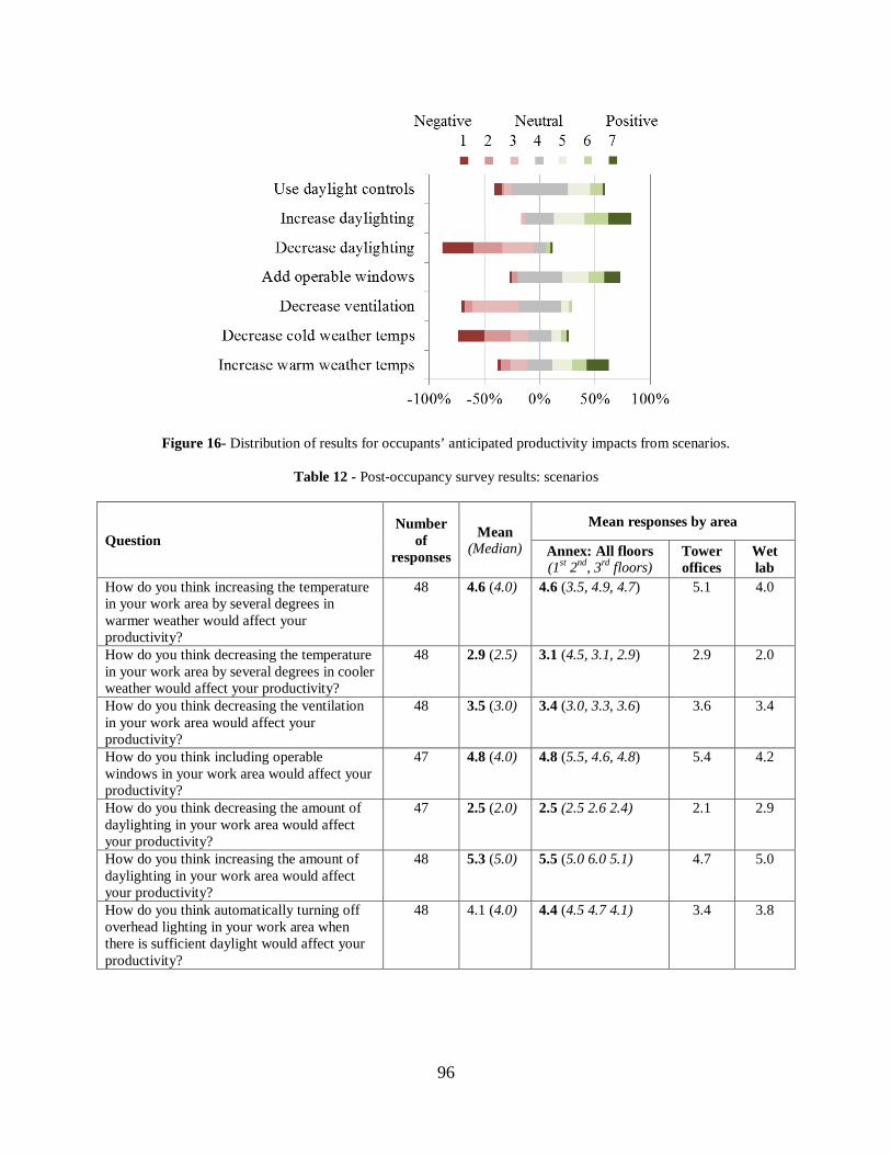
96
Figure 16- Distribution of results for occupants’ anticipated productivity impacts from scenarios.
Table 12 - Post-occupancy survey results: scenarios
Question Number
of responses
Mean (Median)
Mean responses by area
Annex: All floors (1st 2nd, 3rd floors)
Tower offices
Wet lab
How do you think increasing the temperature in your work area by several degrees in warmer weather would affect your productivity?
48 4.6 (4.0) 4.6 (3.5, 4.9, 4.7) 5.1 4.0
How do you think decreasing the temperature in your work area by several degrees in cooler weather would affect your productivity?
48 2.9 (2.5) 3.1 (4.5, 3.1, 2.9) 2.9 2.0
How do you think decreasing the ventilation in your work area would affect your productivity?
48 3.5 (3.0) 3.4 (3.0, 3.3, 3.6) 3.6 3.4
How do you think including operable windows in your work area would affect your productivity?
47 4.8 (4.0) 4.8 (5.5, 4.6, 4.8) 5.4 4.2
How do you think decreasing the amount of daylighting in your work area would affect your productivity?
47 2.5 (2.0) 2.5 (2.5 2.6 2.4) 2.1 2.9
How do you think increasing the amount of daylighting in your work area would affect your productivity?
48 5.3 (5.0) 5.5 (5.0 6.0 5.1) 4.7 5.0
How do you think automatically turning off overhead lighting in your work area when there is sufficient daylight would affect your productivity?
48 4.1 (4.0) 4.4 (4.5 4.7 4.1) 3.4 3.8

97
Raising summer temperatures was rated positively in the Annex and tower offices and
neutral in the wet lab. The anticipated negative effects from lowering winter temperatures or
decreasing daylighting were nearly uniform across building areas, as were the somewhat
negative effects from decreasing ventilation. Increasing daylighting was rated highest in the
Annex, while including operable windows was rated highest in the tower offices. Daylighting
controls were rated positively in the Annex, negatively in the tower offices, and near neutral in
the wet lab.
Results by identifying characteristic - Several of the results were stratified by identifying
characteristics, where evidence from previous studies or the researchers’ judgment suggested a
possible relationship. Choi et al. suggest that “gender matters - increase summer set points”
(Choi et al. 2012). In the MCSI building, the mean satisfaction with temperature in warmer
weather was 2.8 for female occupants (n=12) and 3.9 (n=35) for male occupants, which was
significant at a 90% confidence level (p = 0.07 using a two-tailed t-test assuming unequal
variances). Mean satisfaction in cooler weather was 3.9 for both genders, and 3.5 female/4.1
male overall, though the overall value was not statistically significant. This result corroborates
the findings of Choi et al. Frontczak et al. find that “Office workers will be most satisfied with
their workspace and building when located close to a window in a private office” (Frontczak et
al. 2012). Statistically significant differences were found between open office occupants (n=29)
and private occupants (n=9) for thermal comfort impacts on productivity (p=0.04), air quality
effects on productivity (p=0.001) and overall IEQ impacts on productivity (p=0.05), with the
open office occupants reporting more positive effects for all three questions. No statistically
significant differences were found between open office and private office occupants’ responses
to questions about IEQ perception not related to productivity. These results suggest that in this

98
case, there may be factors other than office type and location that influence occupants’
perception of IEQ impacts on their productivity. Possible factors include job status (e.g. most
open office occupants are graduate students, and most private office occupants are facults), or an
inverted building-specific relationship of office type and percieved IEQ (poorer in the tower
offices). The wet lab area was not included in this comparison.
Overall, the survey results indicated general satisfaction with lighting and daylighting
aspects, and some dissatisfaction with acoustics and thermal comfort aspects, with near neutral
results for air quality. Open-ended responses for possible building improvements included
reducing echoes and mechanical noise, providing better control over temperature including too-
cold temperatures in the summer, mitigating cooking odors from a basement-level restaurant, and
increasing automatic lighting shut-off delay.
Results of the survey were used to qualitatively inform the scenario analysis described in
Chapter 7; i.e. to provide additional support for scenarios which were identified as positive or
neutral – e.g. raising summer temperature set points, using daylighting controls, and demand-
controlled ventilation, but disallowing scenarios that were identified as negative – e.g. lowering
winter temperature set points or reducing ventilation. Operable windows were not able to be
analyzed using the empirical energy model developed herein, whereas general increases or
decreases in daylighting were not considered in the scenario analysis because they would require
extensive modifications to the building.

99
7.0 SCENARIO ANALYSIS: ENERGY-SAVING STRATEGIES
7.1 INTRODUCTION
A scenario analysis was conducted using the IEQ+DLCA model, along with empirically-
derived energy and IEQ relationships for the MCSI building, to explore the tradeoffs or
synergies resulting from changes in building operating parameters. Saving energy - thus reducing
external impacts - while reducing or maintaining constant internal impacts was the main criterion
for the scenarios. Four scenarios were investigated: 1) demand-controlled ventilation (DCV),
which ties outdoor air intake to occupancy levels; 2) raising the cooling season (warm weather)
indoor temperature set point; 3) adding daylighting controls to dim overhead lighting when
adequate daylight was present, and 4) a combined scenario using all three options.
For all scenarios, energy savings were estimated with an empirically-derived energy
model, and IEQ impacts were calculated using parametric relationships developed herein. These
energy savings were input into the DLCA model to calculate the external impacts. Internal
chemical impacts were calculated using the derived building-specific parametric relationships,
and internal non-chemical impacts were limited to ensuring no decrease in relative productivity.

100
7.2 METHODS
The data collection and analysis described in Section 5.1 were used to establish building-
specific parametric relationships. Herein, the development of these relationships is restricted to
the new construction portion, or “annex”. The parametric relationships were used to model the
energy and IEQ consequences of possible building operation scenarios designed to save energy.
Empirical energy model – An empirical energy model was constructed for the MCSI
annex, using the available measurement data. A schematic of the model is shown in Figure 17,
and a summary-level relationship for the model is expressed in Equation 34:
Equation 29
FANHHWSAVENTINTE qqqqqq ,++++=
where qE is the estimated heat gain through the building envelope, qINT is the summary of all
internal heat gains (electrical appliances, lighting, and occupants), qVENT is the heat gain from
conditioning the ventilation (outdoor) air to the internal conditions, qSA is the additional heat gain
from conditioning the supply air (outdoor + recycled), qHW is the hot water space heating gain
(supply air reheat terminals and radiators), and qH,FAN is the heat gain from the supply fan at the
air handler (all q terms are in units of power, typically kW). qSA represents the sum of cooling
coil (chilled water) and heating coil (steam) loads, which are mutually exclusive.

101
Figure 17 - Schematic of parametric energy model for the MCSI Annex
The air handler serving the MCSI annex is a return air system with economizer (Figure
9), which also serves other portions of the Benedum Hall complex. Airflows were measured both
at the air handler and at the variable-air-volume (VAV) units serving the different compartments
of the MCSI space. Loads measured at the air handler (cooling water use, steam use and fan
electrical consumption) were allocated to the MCSI annex by multiplying them by the ratio of
the total airflow at the MCSI VAV units to the total airflow at the air handler. The ventilation
rate was calculated by multiplying the airflow by the economizer percent open, which was
measured by a sensor. During warm weather, the economizer was operated at 20% open.
The variable heat gain associated with ventilation air was calculated using the enthalpy
difference of the outdoor air and indoor air, multiplied by the ventilation mass flow rate. Even at
zero ventilation, further cooling is required in moderate and warm weather to offset heat gain at
the building envelope and indoor thermal loads, such as appliances and occupants, as well as
heat gain introduced by the supply fan. This cooling was calculated using the enthalpy difference

102
of the indoor air and supply air, multiplied by the supply air mass flow rate, and is independent
of the ventilation rate:
Equation 30
OARAOAVENT mhhq *)( −=
where h is the enthalpy of moist air, calculated in accordance with the ASHRAE handbook
(ASHRAE 2009). Assuming conduction through the building envelope as the primary pathway
for the additional cooling, the calculated load was expressed as a function of the temperature
difference between the outdoor and indoor air, and linear regression was used to estimate the
coefficients.
Ventilation and indoor particulate intake - Indoor particle concentrations were observed
to be almost always lower than outdoor concentrations, and to be highly correlated with outdoor
concentrations. Since the building’s MERV 13 air filters are capable of reducing the majority of
PM2.5, it was hypothesized that the ratio of indoor particle levels to outdoor particle counts was
dependent on the status of the economizer. Least-squares regression was performed to establish a
relationship between economizer percent open and indoor/outdoor particle count ratio. This
relationship was used in the subsequent scenario analysis to estimate changes in occupant intake
of particulate matter due to changes in ventilation.
Indoor TVOC emissions - Indoor TVOC emissions were calculated by the same method
used to calculate CO2 emissions and occupancy (Equation 19). Using the measured outdoor and
indoor TVOC concentrations and the airflow rates, a quasi-steady state mass balance model was
used to estimate the TVOC emissions in each compartment as the mass accumulation after
inflow and outflow. TVOC emissions estimated in this way were compared against occupancy
and ventilation rates to determine if any relationship could be found.

103
Scenarios - Four scenarios were investigated: 1) demand-controlled ventilation (DCV),
which ties outdoor air intake to occupancy levels; 2) raising the summer temperature set point by
1.1º C (2º F); 3) adding daylighting controls to dim overhead lighting when adequate daylight
was present, and 4) a combined scenario using all three options. Scenarios and controlling
criteria are outlined in Table 13.
Table 13 - Energy-saving scenarios and controlling criteria
Scenario Controlling parameters Parameter values
1 - DCV Ventilation rate 0.3 l/s/m2 floor area; 45 l/s/person
2 - Summer temperature Indoor temperature set point
Recorded range (Mean 21.5, Std dev 0.88) + 1.1 deg C
3 - Daylighting control Lighting power load
Hourly maximum of: • Actual recorded value • Mean daily minimum +
0.75*mean daily range 4 - Combined All of the above All of the above
For the DCV scenario, inspection of the building operating data, described in detail in the
results section, showed that the building was usually operated at ventilation rates higher than the
upper limits in Equation 25 and Equation 28. The DCV scenario attempted to maintain the
ventilation at 45 l/s/person to achieve maximum productivity according to Eq. 1, given the
occupancy calculated from the CO2 data. An area-specific minimum ventilation rate of 0.3
l/s/(m2 floor area) was added in accordance with ASHRAE Standard 62.1-2010 (ASHRAE
2010).

104
7.3 RESULTS AND DISCUSSION
7.3.1 Building-specific parametric relationships
Energy – Building-specific parametric relationships were developed for the relationship
of envelope heat transfer (QE) and indoor/outdoor temperature difference (Figure 18), and AHU
fan power and mass flow rate (Figure 19).
Figure 18 - MCSI Annex envelope heat transfer as a function of inside-outside temperature difference.

105
Figure 19 - MCSI Annex supply and return fan power as a function of supply air mass flow.
Least-squares regression was used to fit a linear relationship for heat gain and
temperature difference (Equation 31), and a parabolic relationship for supply fan power and mass
flow (Equation 32):
Equation 31
5)(55.12)(*42.3
−>−+−=
io
ioE
TTTTQ
Equation 32
50070.11*1059.1 5
>+×= −
SA
SASF
mmQ
Both relationships were determined to be statistically significant at the 95% level using
the F-test. Although a statistically significant relationship for return fan power was also
established, extrapolating it below the empirically established range resulted in physically
impossible negative values, and therefore it was not used in the scenario analysis.

106
IAQ - The building-specific parametric relationships for ventilation and indoor/outdoor
particle count ratios are shown in Figure 20 and have the form:
Equation 33
bSAOAOutIn mmaPMPM )/(*5.2/5.2 =
where the quantity mOA/mSA is equivalent to the economizer percent open, and the
coefficients a and b varied somewhat between individual compartments in the model, with b
approximately equal to 0.5 in most cases. All of these relationships were determined to be
statistically significant at the 95% level using the F-test. No statistically significant relationships
were found for indoor VOC emissions when evaluated agains either occupancy or ventilation
rate.

107
Figure 20 - Room-level empirical relationships for indoor/outdoor particle count ratio and economizer setting.
7.3.2 Energy savings and life cycle impacts
Figure 21 shows a time-series comparison of the cooling savings from the baseline for
each of the four scenarios. Scenario 1 saved 50% of the building’s ventilation-related cooling
demand, by reducing the ventilation rate generally during hot summer nights, when the building

108
was virtually unoccupied. Even at the relatively high rate of 45 l/s/person used to maintain
productivity in accordance with Equation 25, the summertime maximum (daytime) ventilation
for the rarely exceeded the baseline scenario ventilation. The reduction in ventilation rate
allowed a reduction in the overall supply air demand, reducing supply fan power, with a
corresponding reduction in heating of the supply air stream at the fan (see the recursive loop in
Figure 17). The combined effects of these reductions resulted in a total savings of 11% of total
cooling energy and 6% of total electricity use (from cooling and fans).
Figure 21 - Scenario results for ventilation-related cooling energy consumption from March through October 2012.
Although measured temperatures in occupied spaces rarely varied from a narrow range
around the optimum performance temperature in Equation 27, feedback from the occupant
survey indicated an acceptable increase in space temperature in warmer weather. Scenario 2,
modeling a 1.1º C (2º F) increase in indoor temperature when temperatures outside were higher
than inside, resulted in a 24% reduction in cooling energy and a 9% reduction in total electricity
use. The cooling energy reduction was slightly offset by an increase in supply fan energy to take

109
advantage of the additional range of free cooling. Scenario 3, allowing electric light levels to dim
when daylight was available during cooling season led to an 8% decrease in lighting energy use
and a corresponding 2% decrease in cooling energy use, for a total reduction of 4% of total
electric use. When the three strategies were combined - Scenario 4 - the savings were 8%, 29%,
19% and 14% for lighting, chilled water, supply fan and total electricity respectively.
Monthly time series of IEQ+DLCA model results are shown in Figure 22 for selected
impact categories. External impacts of all types were reduced by decreasing the energy
consumption and generally followed the monthly distribution shown for global warming, for a
total reduction of approximately 14%, with some categories affected slightly more than others by
the timing of the reductions with respect to the dynamic electrical grid mix. The slightly greater
reduction in the photochemical ozone category of 15%, and the different monthly distribution
was due to the use of dynamic CFs from Shah et al. 2008, which are higher in the summer
months, corresponding to the timing of the larger reductions.
Internal respiratory impacts were increased from baseline for all but Scenario 1, because
the lower cooling demand meant that less air recirculation was necessary to meet the cooling
needs at a constant supply air enthalpy. Less air recirculation, while reducing the overall air flow
rate, increased the economizer open percent and increased the average indoor particle count in
accordance with Equation 33 and Figure 20. Increases were 5.5%, 1.8% and 4.5% for Scenarios
2, 3 and 4, respectively. Conversely, estimated internal cancer and noncancer impacts due to
internal VOC sources were reduced by the increased economizer settings in all but Scenario 1.
Changes in these two categories were 22%, -6.3%, -2.1%, and 18% in Scenarios 1, 2, 3 and 4
respectively. From a seasonal standpoint, indoor respiratory impacts were greatest during cool to
110
moderate weather, when outdoor air supply was the greatest, and indoor VOC effects were
greatest during hot weather when outdoor air supply was the lowest.
Figure 23 shows the full summary of results from the IEQ+DLCA model for the study
period, including all external and internal chemical categories. Productivity categories -
absenteeism and at-work performance - are not included in Figure 23 because the baseline
conditions for the MCSI building were near the upper limits for the ventilation-based
relationships, and near the optimum value for the temperature-based relationships included in the
model. A condition of “no change relative to baseline” can be assumed for all scenarios in the
productivity categories. For this case study and time period (~1 year), dynamic variation LCI and
LCIA data did not strongly affect the differences between scenarios. Internal cancer impacts
from indoor sources were sufficiently greater than external cancer impacts, that variations
between scenarios were of the same magnitude as the total external impacts.
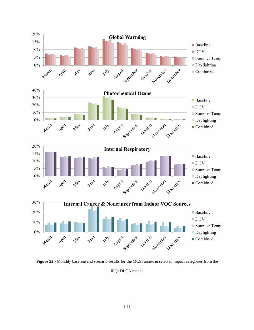
111
Figure 22 - Monthly baseline and scenario results for the MCSI annex in selected impact categories from the
IEQ+DLCA model.

112
Figure 23 - Full LCIA results for the MCSI annex scenario analysis from the IEQ+DLCA model.
Results are normalized to the internal + external total from the baseline scenario.

113
8.0 CONCLUSIONS
8.1 SUMMARY
The goal of this study was to improve LCA methods for whole buildings by developing a
dynamic model and integrating building-level indoor environmental impacts, including both
human health and productivity. The first portion of this study developed the basic dynamic LCA
(DLCA) framework and illustrated the potential importance of the method using a simplified
retrospective and prospective case study of an institutional building (Benedum Hall). The results
showed that the environmental impacts of the building over its lifetime varied from what would
be predicted if temporal changes were not taken into account. Particularly, the results indicated
the importance of changes in building usage, energy sources and environmental regulations in
calculating the overall environmental impacts of the building. Given that temporal changes are
rarely accounted for in LCA practice, it seems clear that LCA could be improved by moving to a
more dynamic framework. Previous whole-building LCAs have demonstrated the relative
importance of the operations phase in most impact categories, compared to the materials,
construction and end-of-life phases. The DLCA results suggested an additional conclusion; that
in some cases, changes in building usage, or changes in external conditions such as energy mixes
or environmental regulations during a building’s lifetime, can influence the LCA results to a
greater degree than the material and construction phases. Correspondingly, adapting LCA to a

114
more dynamic approach as demonstrated herein seems likely to increase the usefulness of the
method in assessing the performance of buildings and other complex systems in the built
environment.
The second portion of this work outlined a framework for including whole-building IEQ
effects in LCA. The framework added three types of impacts to the LCA matrix: internal
chemical impacts, internal non-chemical health impacts, and performance/productivity impacts.
Indoor chemical impacts included impacts from indoor emissions as well as the intake of outdoor
pollution. Indoor chemical impacts were categorized so as to be directly comparable to existing
LCIA categories, which are conventionally used for external impacts only. These categories are
respiratory effects, cancer toxicity and noncancer toxicity. Indoor nonchemical impacts were
disaggregated into health and productivity impacts. After analysis of the potential overlap
between chemical-specific health effects and the remaining health effects, it was concluded that
some categories of nonchemical health impacts (e.g. SBS) could not be included in the
framework without potential double-counting. Furthermore, the remaining nonchemical health
impacts (e.g. BRI and impacts not related to air quality) have not been studied sufficiently to
permit the development of empirical parametric relationships for inclusion in the framework.
However, productivity impacts related to absenteeism and at-work performance were able to be
included, and could potentially capture some of the missing health impacts.
The complete IEQ+DLCA framework was evaluated using a case study of a LEED Gold
academic building - the MCSI building at the University of Pittsburgh, a combination annex to
and renovation of a portion of Benedum Hall, the subject of the first case study. Extensive data
were collected on energy consumption and IEQ variables, and a post-occupancy survey was
performed to evaluate occupant perceptions of IEQ and its effects on productivity. Results of the

115
case study suggest that in some instances, internal effects can be comparable to internal effects.
For internal building respiratory effects, the performance of the mechanical filtration system can
influence the results by several orders of magnitude. For example, although the internal
respiratory effects in this study were lower than the external respiratory effects, they would have
been greater without the building’s MERV 13 filters; for instance, many commercial buildings
may only employ a MERV 8 filter, which has minimal removal of PM2.5. An illustrative
scenario of a lower-performing building showed that internal effects could be greater than
external effects in some cases. This could be due to some combination of poor filtration and/or
indoor sources of particulate matter. For cancer toxicity, the estimated internal effects were
greater than external effects. In other words, the estimated exposure of building occupants, even
in a building achieving LEED certification, could be greater than the total exposure of external
populations due to the upstream processes of the building’s operating energy supply.
Indoor source control via low-VOC building materials, furnishings and maintenance
items is believed to be very important for VOC exposure; this was corroborated by the relatively
low indoor contribution to TVOC levels for the case study building compared to the BASE
study. This was expected since as a LEED Gold building the case study was designed with
indoor source control as a key element. Ventilation complements indoor source control by
removing internally generated pollutants from both occupants and building materials; however,
increased ventilation without much greater attention to filtration or other treatment of outdoor
and recirculated air carries the risk of increased impacts in some categories (e.g., respiratory
effects and non-carcinogenic toxicity) offsetting gains in other categories (e.g. carcinogens).
These relationships are site-specific, so tradeoffs will vary on a case-by-case basis. Incorporating
both chemical and non-chemical health and productivity impacts into the IEQ+DLCA

116
framework demonstrated the need to carefully consider IEQ consequences when making
decisions related to energy savings. Limits on operational changes were revealed, underscoring
the potential importance of design features.
The post-occupancy survey supplemented the physical analysis of the building and the
existing literature on occupants’ perceptions of IEQ and its relationship to their productivity.
Previously documented relationships between IEQ and productivity indicate a positive
correlation with ventilation and an optimal temperature range. However, the survey results
suggested some degree of flexibility with respect to indoor temperature set points during the
cooling season, which corresponded with the results of another previous qualitative study.
Daylighting was confirmed to be a critical variable for IEQ satisfaction. As with the chemical
impacts, the non-chemical health and productivity impacts may be site and population-specific,
varying with the setting and occupant type, even when building design features are similar.
8.2 FUTURE WORK
Future research needs include aspects of both the dynamic features and IEQ categories in
LCA, as well as refinements to the underlying human health functions. For DLCA, additional
needs are characterization of uncertainty related to building systems modeling (e.g. future
occupant needs and maintenance/renovation schedules); additional exploration of the interactions
with dynamic, temporally evolving (and themselves uncertain) LCI and LCIA background
variables; and development of additional dynamic CFs and dynamic parameters for LCI
databases. The variability in these tradeoffs may support greater attention to the development of

117
more sophisticated building modeling and the application of regional criteria in green building
rating systems.
With respect to IEQ, overlaps between chemical-specific, toxicologically-based effect
factors from LCIA methods, and empirically derived relationships from the IAQ literature,
indicate a need for interdisciplinary efforts targeted at merging the two knowledge bases. There
is a need for serious consideration of threshold doses in LCIA models so that insignificant
increases in impact can be excluded as negligible.
Future work on the current project includes the exploration of an additional high-
performance building case study - the Center for Sustainable Landscapes at Phipps Conservatory
in Pittsburgh, as well as the continued development of the IEQ+DLCA model toward a building-
level dashboard system, with improvements from both a sensing and computational standpoint.
A long-term goal is to develop a reference set of estimates using data from studies such as this
and the BASE study to provide design-level estimates of the tradeoffs between internal and
external impacts.
8.3 OUTLOOK
Overall, LCA could be improved as a design tool for whole buildings by including a
thorough analysis of the IEQ effects of design decisions, as well as internal and external system
changes over a building’s lifetime. Understanding the uncertainties with respect to both LCIA
internal building results and external (conventional) LCA results, we conclude that for LCA of
whole buildings, including dynamic modeling and building-level IEQ categories is important.
The findings of this study, while underscoring the importance of internal impacts, may support

118
the use of green building rating systems, which include the benefits of enhanced IEQ from better
filtration, indoor chemical source control and attention to non-chemical environmental variables
such as lighting and acoustics. As these impacts accrue to different populations (building
occupants versus the world at large), the overall vision is to reduce environmental impacts
related to the built environment.

119
APPENDIX A
INPUTS AND RESULTS FOR INITIAL DLCA CASE STUDY
A.1 BUILDING MATERIAL AND ENERGY DATA

120
Table 14 - Actual and estimated energy data for Benedum Hall.
Month and Year
Boiler Plant Data Benedum Hall Consumption eQUEST Simulated Data(4)
Steam Generation (Gg)
Coal for steam (Gg)
Gas for steam (106 m3)
Steam energy content (MJ/kg)(1)
Steam (Mg)(3)
Electricity (MWh)(3)
Steam (GJ)(3)
Steam (Mg)
Electricity (MWh)
Steam (GJ)
Jul‐92 ‐‐‐ ‐‐‐ ‐‐‐ ‐‐‐(2) 260 1090 690 400 1060 1060 Aug‐92 ‐‐‐ ‐‐‐ ‐‐‐ ‐‐‐ 250 820 670 401 1090 1060 Sep‐92 ‐‐‐ ‐‐‐ ‐‐‐ ‐‐‐ 210 1050 580 591 1130 1650 Oct‐92 ‐‐‐ ‐‐‐ ‐‐‐ ‐‐‐ 410 860 1090 589 930 1570 Nov‐92 ‐‐‐ ‐‐‐ ‐‐‐ ‐‐‐ 710 880 1850 867 800 2260 Dec‐92 ‐‐‐ ‐‐‐ ‐‐‐ ‐‐‐ 980 790 2550 1324 780 3430 Jan‐93 ‐‐‐ ‐‐‐ ‐‐‐ ‐‐‐ 1010 750 2640 1673 720 4370 Feb‐93 ‐‐‐ ‐‐‐ ‐‐‐ ‐‐‐ 1030 840 2700 1536 740 4050 Mar‐93 ‐‐‐ ‐‐‐ ‐‐‐ ‐‐‐ 810 870 2100 885 920 2300 Apr‐93 ‐‐‐ ‐‐‐ ‐‐‐ ‐‐‐ 520 870 1420 546 910 1490 May‐93 ‐‐‐ ‐‐‐ ‐‐‐ ‐‐‐ 320 810 860 413 870 1130 Jun‐93 ‐‐‐ ‐‐‐ ‐‐‐ ‐‐‐ 250 1010 740 394 1050 1150 Jul‐93 ‐‐‐ ‐‐‐ ‐‐‐ ‐‐‐ 180 1170 480 398 1060 1060 Aug‐93 ‐‐‐ ‐‐‐ ‐‐‐ ‐‐‐ 210 1070 560 401 1090 1060 Sep‐93 ‐‐‐ ‐‐‐ ‐‐‐ ‐‐‐ 220 1080 620 591 1130 1650 Oct‐93 ‐‐‐ ‐‐‐ ‐‐‐ ‐‐‐ 380 880 1010 589 930 1570 Nov‐93 ‐‐‐ ‐‐‐ ‐‐‐ ‐‐‐ 710 840 1850 867 800 2260 Dec‐93 ‐‐‐ ‐‐‐ ‐‐‐ ‐‐‐ 1220 800 3160 1324 780 3430 Jan‐94 ‐‐‐ ‐‐‐ ‐‐‐ ‐‐‐ 1340 830 3490 1673 720 4370 Feb‐94 ‐‐‐ ‐‐‐ ‐‐‐ ‐‐‐ 1000 860 2630 1536 740 4050 Mar‐94 ‐‐‐ ‐‐‐ ‐‐‐ ‐‐‐ 750 1050 1940 885 920 2300 Apr‐94 ‐‐‐ ‐‐‐ ‐‐‐ ‐‐‐ 430 930 1160 546 910 1490 May‐94 ‐‐‐ ‐‐‐ ‐‐‐ ‐‐‐ 380 890 1030 413 870 1130 Jun‐94 ‐‐‐ ‐‐‐ ‐‐‐ ‐‐‐ 290 1190 840 394 1050 1150 Jul‐94 ‐‐‐ ‐‐‐ ‐‐‐ ‐‐‐ 290 940 780 398 1060 1060 Aug‐94 ‐‐‐ ‐‐‐ ‐‐‐ ‐‐‐ 330 1040 860 401 1090 1060 Sep‐94 ‐‐‐ ‐‐‐ ‐‐‐ ‐‐‐ 250 900 710 591 1130 1650 Oct‐94 ‐‐‐ ‐‐‐ ‐‐‐ ‐‐‐ 320 790 860 589 930 1570 Nov‐94 ‐‐‐ ‐‐‐ ‐‐‐ ‐‐‐ 500 900 1310 867 800 2260 Dec‐94 ‐‐‐ ‐‐‐ ‐‐‐ ‐‐‐ 720 630 1860 1324 780 3430 Jan‐95 ‐‐‐ ‐‐‐ ‐‐‐ ‐‐‐ 1010 820 2640 1673 720 4370 Feb‐95 ‐‐‐ ‐‐‐ ‐‐‐ ‐‐‐ 1010 710 2670 1536 740 4050 Mar‐95 ‐‐‐ ‐‐‐ ‐‐‐ ‐‐‐ 850 970 2200 885 920 2300 Apr‐95 ‐‐‐ ‐‐‐ ‐‐‐ ‐‐‐ 610 790 1650 546 910 1490 May‐95 ‐‐‐ ‐‐‐ ‐‐‐ ‐‐‐ 280 750 780 413 870 1130 Jun‐95 ‐‐‐ ‐‐‐ ‐‐‐ ‐‐‐ 230 1100 680 394 1050 1150 Jul‐95 ‐‐‐ ‐‐‐ ‐‐‐ ‐‐‐ 230 890 600 398 1060 1060 Aug‐95 ‐‐‐ ‐‐‐ ‐‐‐ ‐‐‐ 180 1170 480 401 1090 1060 Sep‐95 ‐‐‐ ‐‐‐ ‐‐‐ ‐‐‐ 170 920 480 591 1130 1650 Oct‐95 ‐‐‐ ‐‐‐ ‐‐‐ ‐‐‐ 360 870 970 589 930 1570 Nov‐95 ‐‐‐ ‐‐‐ ‐‐‐ ‐‐‐ 900 880 2350 867 800 2260 Dec‐95 ‐‐‐ ‐‐‐ ‐‐‐ ‐‐‐ 1150 720 2990 1324 780 3430 Jan‐96 ‐‐‐ ‐‐‐ ‐‐‐ ‐‐‐ 1210 650 3150 1673 720 4370 Feb‐96 ‐‐‐ ‐‐‐ ‐‐‐ ‐‐‐ 1010 810 2670 1536 740 4050 Mar‐96 ‐‐‐ ‐‐‐ ‐‐‐ ‐‐‐ 970 720 2520 885 920 2300 Apr‐96 ‐‐‐ ‐‐‐ ‐‐‐ ‐‐‐ 580 720 1580 546 910 1490 May‐96 ‐‐‐ ‐‐‐ ‐‐‐ ‐‐‐ 320 800 880 413 870 1130 Jun‐96 ‐‐‐ ‐‐‐ ‐‐‐ ‐‐‐ 230 850 670 394 1050 1150 Jul‐96 ‐‐‐ ‐‐‐ ‐‐‐ ‐‐‐ 230 1080 620 398 1060 1060 Aug‐96 ‐‐‐ ‐‐‐ ‐‐‐ ‐‐‐ 250 820 670 401 1090 1060

121
Table 14 (Continued)
Sep‐96 ‐‐‐ ‐‐‐ ‐‐‐ ‐‐‐ 330 840 910 591 1130 1650 Oct‐96 ‐‐‐ ‐‐‐ ‐‐‐ ‐‐‐ 420 930 1130 589 930 1570 Nov‐96 ‐‐‐ ‐‐‐ ‐‐‐ ‐‐‐ 950 700 2470 867 800 2260 Dec‐96 ‐‐‐ ‐‐‐ ‐‐‐ ‐‐‐ 990 720 2560 1324 780 3430 Jan‐97 ‐‐‐ ‐‐‐ ‐‐‐ ‐‐‐ 1020 870 2660 1673 720 4370 Feb‐97 ‐‐‐ ‐‐‐ ‐‐‐ ‐‐‐ 860 710 2260 1536 740 4050 Mar‐97 ‐‐‐ ‐‐‐ ‐‐‐ ‐‐‐ 790 810 2050 885 920 2300 Apr‐97 ‐‐‐ ‐‐‐ ‐‐‐ ‐‐‐ 610 870 1660 546 910 1490 May‐97 ‐‐‐ ‐‐‐ ‐‐‐ ‐‐‐ 320 760 880 413 870 1130 Jun‐97 ‐‐‐ ‐‐‐ ‐‐‐ ‐‐‐ 310 790 890 394 1050 1150 Jul‐97 ‐‐‐ ‐‐‐ ‐‐‐ ‐‐‐ 340 1020 900 398 1060 1060 Aug‐97 ‐‐‐ ‐‐‐ ‐‐‐ ‐‐‐ 300 810 790 401 1090 1060 Sep‐97 ‐‐‐ ‐‐‐ ‐‐‐ ‐‐‐ 320 970 890 591 1130 1650 Oct‐97 ‐‐‐ ‐‐‐ ‐‐‐ ‐‐‐ 510 840 1370 589 930 1570 Nov‐97 ‐‐‐ ‐‐‐ ‐‐‐ ‐‐‐ 870 770 2260 867 800 2260 Dec‐97 ‐‐‐ ‐‐‐ ‐‐‐ ‐‐‐ 1000 830 2580 1324 780 3430 Jan‐98 ‐‐‐ ‐‐‐ ‐‐‐ ‐‐‐ 970 740 2520 1673 720 4370 Feb‐98 ‐‐‐ ‐‐‐ ‐‐‐ ‐‐‐ 880 770 2330 1536 740 4050 Mar‐98 ‐‐‐ ‐‐‐ ‐‐‐ ‐‐‐ 820 890 2140 885 920 2300 Apr‐98 ‐‐‐ ‐‐‐ ‐‐‐ ‐‐‐ 400 840 1080 546 910 1490 May‐98 ‐‐‐ ‐‐‐ ‐‐‐ ‐‐‐ 200 790 550 413 870 1130 Jun‐98 ‐‐‐ ‐‐‐ ‐‐‐ ‐‐‐ 180 850 520 394 1050 1150 Jul‐98 ‐‐‐ ‐‐‐ ‐‐‐ ‐‐‐ 200 1080 530 398 1060 1060 Aug‐98 ‐‐‐ ‐‐‐ ‐‐‐ ‐‐‐ 290 970 760 401 1090 1060 Sep‐98 ‐‐‐ ‐‐‐ ‐‐‐ ‐‐‐ 290 1030 800 591 1130 1650 Oct‐98 ‐‐‐ ‐‐‐ ‐‐‐ ‐‐‐ 480 930 1290 589 930 1570 Nov‐98 ‐‐‐ ‐‐‐ ‐‐‐ ‐‐‐ 960 920 2490 867 800 2260 Dec‐98 ‐‐‐ ‐‐‐ ‐‐‐ ‐‐‐ 960 910 2490 1324 780 3430 Jan‐99 ‐‐‐ ‐‐‐ ‐‐‐ ‐‐‐ 1280 760 3350 1673 720 4370 Feb‐99 ‐‐‐ ‐‐‐ ‐‐‐ ‐‐‐ 1060 940 2800 1536 740 4050 Mar‐99 ‐‐‐ ‐‐‐ ‐‐‐ ‐‐‐ 1290 920 3360 885 920 2300 Apr‐99 ‐‐‐ ‐‐‐ ‐‐‐ ‐‐‐ 680 850 1860 546 910 1490 May‐99 ‐‐‐ ‐‐‐ ‐‐‐ ‐‐‐ 540 890 1460 413 870 1130 Jun‐99 ‐‐‐ ‐‐‐ ‐‐‐ ‐‐‐ 410 1120 1200 394 1050 1150 Jul‐99 ‐‐‐ ‐‐‐ ‐‐‐ ‐‐‐ 460 980 1230 398 1060 1060 Aug‐99 ‐‐‐ ‐‐‐ ‐‐‐ ‐‐‐ 460 1070 1220 401 1090 1060 Sep‐99 ‐‐‐ ‐‐‐ ‐‐‐ ‐‐‐ 610 1130 1700 591 1130 1650 Oct‐99 ‐‐‐ ‐‐‐ ‐‐‐ ‐‐‐ 910 1010 2430 589 930 1570 Nov‐99 ‐‐‐ ‐‐‐ ‐‐‐ ‐‐‐ 980 940 2540 867 800 2260 Dec‐99 ‐‐‐ ‐‐‐ ‐‐‐ ‐‐‐ 1310 1040 3400 1324 780 3430 Jan‐00 98.61 4.95 3.49 2.61 1420 1020 3690 1676 720 4370 Feb‐00 79.11 4.33 2.86 2.75 1610 1010 4420 1475 740 4050 Mar‐00 65.13 4.53 1.71 2.73 1280 1130 3510 841 920 2300 Apr‐00 50.85 3.25 1.61 2.80 1220 950 3420 531 910 1490 May‐00 31.77 2.21 1.06 3.01 760 860 2290 375 870 1130 Jun‐00 24.28 1.65 0.91 3.13 420 1170 1310 367 1050 1150 Jul‐00 27.34 1.26 1.15 2.76 460 940 1260 382 1060 1060 Aug‐00 26.64 1.14 1.15 2.72 440 1060 1200 389 1090 1060 Sep‐00 28.95 1.56 1.18 2.91 510 1040 1480 566 1130 1650 Oct‐00 46.17 3.21 1.31 2.82 730 980 2060 558 930 1570 Nov‐00 73.27 4.45 2.23 2.67 1450 910 3890 844 800 2260 Dec‐00 107.17 6.04 3.75 2.75 1510 860 4160 1249 780 3430 Jan‐01 99.28 6.33 2.73 2.64 1660 950 4370 1655 720 4370 Feb‐01 80.34 5.18 2.08 2.60 1390 890 3610 1558 740 4050

122
Table 14 (Continued)
Mar‐01 85.55 4.90 2.15 2.39 1440 880 3440 963 920 2300 Apr‐01 51.18 3.40 1.29 2.62 840 1120 2190 568 910 1490 May‐01 35.89 2.66 0.71 2.60 720 890 1880 434 870 1130 Jun‐01 27.76 1.73 0.76 2.61 410 1150 1060 441 1050 1150 Jul‐01 25.88 1.87 0.52 2.57 400 940 1030 410 1060 1060 Aug‐01 24.45 1.46 0.72 2.61 450 1140 1170 405 1090 1060 Sep‐01 28.88 1.40 1.06 2.61 540 1040 1400 630 1130 1650 Oct‐01 47.63 3.11 1.20 2.59 900 930 2330 606 930 1570 Nov‐01 56.74 3.71 1.38 2.56 1010 900 2590 883 800 2260 Dec‐01 78.12 5.60 1.56 2.55 1140 800 2910 1344 780 3430 Jan‐02 86.31 6.18 1.82 2.59 1350 1070 3500 1689 720 4370 Feb‐02 79.40 5.03 2.05 2.57 1220 630 3120 1579 740 4050 Mar‐02 76.95 5.30 1.92 2.67 1160 850 3100 862 920 2300 Apr‐02 54.70 4.06 1.30 2.76 1300 1090 3570 540 910 1490 May‐02 45.66 3.15 1.04 2.59 1140 350 2950 435 870 1130 Jun‐02 29.59 2.28 0.86 3.03 540 1030 1630 380 1050 1150 Jul‐02 25.54 1.17 0.99 2.62 90 940 230 402 1060 1060 Aug‐02 26.65 1.29 0.95 2.57 190 1100 480 410 1090 1060 Sep‐02 25.48 1.59 0.85 2.83 190 1060 540 581 1130 1650 Oct‐02 53.47 3.36 1.44 2.60 930 920 2420 606 930 1570 Nov‐02 74.67 5.30 1.58 2.58 1280 850 3300 875 800 2260 Dec‐02 97.35 5.79 2.52 2.47 1870 810 4630 1387 780 3430 Jan‐03 115.57 6.08 3.37 2.43 2300 820 5590 1800 720 4370 Feb‐03 99.65 5.38 3.05 2.52 2140 810 5380 1609 740 4050 Mar‐03 77.02 5.03 1.98 2.61 1820 660 4760 881 920 2300 Apr‐03 53.68 3.80 1.31 2.70 1470 560 3970 551 910 1490 May‐03 41.78 3.23 0.91 2.76 940 990 2600 410 870 1130 Jun‐03 33.26 2.50 0.91 2.92 560 1320 1650 394 1050 1150 Jul‐03 28.59 2.06 0.93 3.05 530 850 1620 346 1060 1060 Aug‐03 30.07 1.88 0.97 2.79 570 1000 1580 378 1090 1060 Sep‐03 34.31 2.11 1.00 2.65 690 950 1830 621 1130 1650 Oct‐03 55.79 3.52 1.34 2.49 1190 900 2980 630 930 1570 Nov‐03 65.11 4.48 1.54 2.62 1250 850 3270 861 800 2260 Dec‐03 96.29 5.96 2.60 2.58 2030 780 5220 1331 780 3430 Jan‐04 118.24 6.12 4.09 2.61 2160 820 5660 1671 720 4370 Feb‐04 95.15 5.84 2.54 2.55 1940 800 4940 1590 740 4050 Mar‐04 78.54 5.48 2.02 2.72 1560 560 4250 845 920 2300 Apr‐04 59.64 4.51 1.22 2.66 1190 560 3170 558 910 1490 May‐04 38.68 2.71 0.78 2.51 640 560 1610 449 870 1130 Jun‐04 31.46 2.20 0.75 2.65 330 560 880 433 1050 1150 Jul‐04 27.97 1.79 0.84 2.75 130 670 350 383 1060 1060 Aug‐04 29.71 1.52 1.00 2.56 160 1000 400 413 1090 1060 Sep‐04 30.66 1.60 0.98 2.53 300 950 750 651 1130 1650 Oct‐04 46.02 3.16 1.16 2.67 970 900 2590 588 930 1570 Nov‐04 65.31 4.33 1.61 2.59 1480 850 3840 870 800 2260 Dec‐04 94.89 5.80 2.78 2.64 1930 780 5100 1298 780 3430 Jan‐05 106.15 5.61 3.79 2.68 2110 720 5660 1628 720 4370 Feb‐05 89.25 5.00 3.28 2.80 1830 810 5120 1446 740 4050 Mar‐05 94.94 4.74 3.46 2.64 1790 560 4730 871 920 2300 Apr‐05 55.96 2.85 2.14 2.73 960 560 2620 544 910 1490 May‐05 46.00 2.31 1.65 2.62 920 560 2420 431 870 1130 Jun‐05 32.32 1.64 1.12 2.59 490 560 1260 444 1050 1150 Jul‐05 33.29 2.15 0.75 2.47 360 560 900 427 1060 1060 Aug‐05 33.16 2.18 0.71 2.46 350 1000 860 428 1090 1060

123
Table 14 (Continued)
Sep‐05 35.52 2.45 0.80 2.57 380 920 980 640 1130 1650 Oct‐05 52.88 2.80 1.80 2.62 1010 900 2650 599 930 1570 Nov‐05 73.06 4.16 2.35 2.65 1260 900 3350 852 800 2260 Dec‐05 108.15 5.03 4.33 2.69 2150 890 5800 1274 780 3430 Jan‐06 90.78 4.23 3.50 2.64 1720 860 4550 1655 720 4370 Feb‐06 95.60 4.16 3.85 2.63 1700 830 4470 1541 740 4050 Mar‐06 88.14 4.35 3.28 2.65 1490 920 3960 867 920 2300 Apr‐06 57.02 3.31 1.87 2.70 890 920 2400 551 910 1490 May‐06 46.73 2.69 1.45 2.62 710 900 1850 431 870 1130 Jun‐06 36.58 2.11 1.17 2.67 380 810 1000 431 1050 1150 Jul‐06 35.51 2.40 1.06 2.83 360 800 1020 373 1060 1060 Aug‐06 34.77 2.14 1.06 2.69 330 880 900 392 1090 1060 Sep‐06 38.82 2.50 1.12 2.71 370 880 1010 607 1130 1650 Oct‐06 59.15 3.92 1.76 2.79 910 910 2530 564 930 1570 Nov‐06 71.48 3.21 2.61 2.52 1170 950 2940 896 800 2260 Dec‐06 86.54 4.68 2.95 2.65 850 840 2250 1293 780 3430 Jan‐07 84.52 4.78 2.80 2.68 960 880 2580 1631 720 4370 Feb‐07 110.86 4.53 4.68 2.64 1090 950 2880 1537 740 4050 Mar‐07 84.37 4.65 2.93 2.70 800 930 2160 851 920 2300 Apr‐07 70.26 4.46 2.00 2.67 720 910 1920 557 910 1490 May‐07 45.59 3.04 1.15 2.63 360 970 930 430 870 1130 Jun‐07 37.27 2.68 0.97 2.78 280 810 770 414 1050 1150 Jul‐07 35.00 2.46 0.91 2.74 230 800 620 384 1060 1060 Aug‐07 33.79 2.28 0.94 2.74 190 880 520 384 1090 1060 Sep‐07 35.44 1.74 1.33 2.66 210 870 570 618 1130 1650 Oct‐07 47.27 2.34 1.68 2.59 400 1020 1030 606 930 1570 Nov‐07 79.30 4.35 2.72 2.68 810 920 2180 843 800 2260 Dec‐07 105.27 5.69 3.67 2.68 1080 860 2900 1278 780 3430 Jan‐08 100.10 5.28 3.52 2.66 1100 950 2920 1642 720 4370 Feb‐08 98.39 4.96 3.59 2.65 990 960 2630 1528 740 4050 Mar‐08 103.33 5.36 3.66 2.65 960 880 2530 868 920 2300 Apr‐08 66.85 3.98 1.99 2.62 570 990 1500 567 910 1490 May‐08 55.46 3.36 1.71 2.69 310 850 830 420 870 1130 Jun‐08 40.88 2.62 1.22 2.74 140 840 370 420 1050 1150 Jul‐08 40.51 2.54 1.43 2.91 110 940 330 362 1060 1060 Aug‐08 40.79 2.14 1.30 2.53 120 830 300 418 1090 1060 Sep‐08 41.56 2.42 1.20 2.55 50 890 120 644 1130 1650 Oct‐08 65.33 3.49 2.26 2.66 350 980 920 592 930 1570 Nov‐08 93.61 4.81 3.45 2.69 600 820 1620 839 800 2260 Dec‐08 117.56 5.81 4.46 2.69 840 800 2260 1277 780 3430 Jan‐09 105.32 5.47 3.63 2.61 1880 950 4900 2519 750 6580 Feb‐09 88.84 4.63 3.00 2.59 1260 1740 3270 2583 780 6690 Mar‐09 97.21 4.82 3.37 2.57 1260 560 3250 1562 960 4010 Apr‐09 74.93 4.18 2.28 2.56 760 910 1940 1123 940 2870 May‐09 53.89 3.32 1.48 2.59 610 770 1570 624 900 1610 Jun‐09 38.79 1.91 1.50 2.70 390 850 1070 527 1130 1420 Jul‐09 44.35 0 3.30 2.86 370 990 1060 468 1130 1340 Aug‐09 40.33 0 2.99 2.85 290 910 830 445 1170 1270 Sep‐09 45.07 0 3.19 2.71 290 700 780 801 1200 2170 Oct‐09 69.24 0 5.18 2.87 550 1360 1580 977 970 2810 Nov‐09 70.60 0 5.14 2.79 840 930 2340 1488 830 4160 Dec‐09 68.76 0 5.05 2.82 1430 1050 4030 1988 810 5600 Jan‐10 77.89 0 5.75 2.83 1810 920 5140 2323 750 6580 Feb‐10 73.55 0 5.42 2.83 4470 920 12620 2367 780 6690

124
Table 14 (Continued)
Mar‐10 52.58 0 3.79 2.77 1860 920 5150 1449 960 4010 Apr‐10 36.03 0 2.57 2.74 1410 1090 3860 1048 940 2870 May‐10 25.21 0 1.83 2.79 1270 920 3530 579 900 1610 Jun‐10 24.79 0 1.79 2.76 1040 1060 2870 515 1130 1420 Jul‐10 24.51 0 1.75 2.74 1050 1030 2880 489 1130 1340 Aug‐10 22.08 0 1.52 2.65 1100 980 2900 478 1170 1270 Sep‐10 25.37 0 1.95 2.95 1150 1050 3390 737 1200 2170 Oct‐10 43.49 0 3.21 2.83 1460 960 4140 992 970 2810 Nov‐10 59.39 0 4.42 2.85 2170 1010 6210 1456 830 4160 Dec‐10 80.70 0 5.99 2.85 2900 1030 8260 1968 810 5600 Jan‐11 78.21 0 5.76 2.83 3020 970 8540 2330 750 6580 Feb‐11 61.29 0 4.48 2.81 2460 1000 6910 2384 780 6690
Table 14 Notes:
1) Steam energy content was calculated using values of 24.8 MJ/kg for coal and 38.4 MJ/m3 for gas. This represents primary energy content and includes all energy losses during steam generation, distribution and use. 2) For the years 1971 through 1999, steam energy content was assumed to be the average of years 2000‐2002 on a
month‐by‐month basis. 3) For the years 1971 through June 1992, electrical and steam usage were assumed to be the average of years 1993‐
1995 on a month‐by‐month basis. 4) The eQUEST model was constructed for the original building and compared with actual data from years 1993‐
2001 (prior to removal of electric chillers from the building's roof). Once this model was completed, the renovation changes were added and results of the renovated building model were used from March 2011 onward.
Figure 24 - Comparison of actual electrical usage and eQUEST model results for Benedum Hall.
Actual usage from 2002-2011 does not include cooling since the building was connected to the central campus
chilled water plant in 2002.

125
Figure 25 - Comparison of steam usage and eQUEST model results for Benedum Hall

126
A.2 LIFE CYCLE INVENTORY
Table 15 - Mass and embodied energy inputs for static LCA model of Benedum Hall materials compared to two
other studies
Case Study: Benedum Hall Scheuer 2003 Junnila 2006
Building lifetime
75 Years Building lifetime 75 Years Building lifetime
50 Years
Floor area 37,000 m2 Floor area 7,300 m2 Floor area 4,400 m2
Mass/area (kg/m2)
Energy/area (MJ/m2)
Materials Mass/area (kg/m2)
Energy/area (MJ/m2)
Materials Energy/area (MJ/m2)
Structural steel (piling and rebar)
77 1,870 Steel, electric arc furnace
65 790 Rebar and steel stairs
1,080
Structural concrete
1180 820 Cement (in concrete) Sand (concrete and backfill) Gravel (concrete)
180 1100 320
670 660 64
Concrete 700
Concrete masonry unit walls
250 190 NA2 NA NA NA NA
Steel studs, doors, and frames3
22 600 Steel, primary, cold rolled Steel, secondary, hot rolled
12 10
322 139
Steel studs, doors, frames and grid
890
Steel piping and ductwork (galvanized and stainless)
18 600 Steel, primary, electrogalvanized
10
319
Steel, piping and ductwork
1,400
Cast iron piping3
6.7 160 Cast iron 6.7 220 Incl. in steel piping
NA
Copper tubing and wire3
4.5 140 Copper, primary, extruded Copper tube
2.9 1.6
206 108
Copper tubing and wire
250
Aluminum (window frames, cladding panels)
0.49 56 Aluminum, primary
2.1 425 Aluminum 18
Exterior masonry (limestone)
86 2.4 Exterior masonry (brick)
53 143 NA NA
Resilient floor tile
3.2 190 NA NA NA Ceramic tile 250
Glass (windows)
5.5 71 Glass 6.4 44 Glass 780
Gypsum board
5.4 31 Kraft paper Gypsum, primary Gypsum, secondary
8.4 10 10
315 8 0
Gypsum board Mineral fiber board ceiling tile
340 210

127
Table 15 (Continued)
Extruded polystyrene insulation
0.19 20 Polyisocyanurate Polystyrene
1.2 0.8
86 78
Extruded polystyrene insulation
20
Fiberglass insulation
0.45 21 Glass fiber, primary
2.9 51 Fiberglass insulation
710
HVAC multizone units
10 270 NA NA NA HVAC multizone units
420
GFRC panels 0.04 0.14 NA NA NA NA NA Polyethylene (cladding panels)
0.2 16 NA NA NA NA NA
Total materials
1670 5,080 Total materials 2,000 6,250 Total materials
11,900
Original construction materials
1570 4,250 Original construction materials
7,060
Renovation materials
100 820 Renovation materials
4,860
Total shown here4 1,780 4,640 Total shown here4
7,100
% Total shown here
90% 74% % Total shown here
59%
Total operating energy
3,920 Total operating energy
4,100 Total operating energy
1,360
Electricity 3,340 700 Heating 580 660
Table 15 Notes:
1.This table attempts to provide comparable items in rows going across, where possible. There is overlap between
some categories across the studies, but not within studies.
2. NA = Not applicable - generally, not present in the subject building.
3. Values from Scheuer et al. for mass/area were used herein for these material categories.
4. Major items excluded from “Total shown here” are the following: For Scheuer et al. - carpet, roofing materials,
fireproofing and paint; For Junnila et al. - carpet, roofing materials, ceiling tile, elevator and paint. Fireproofing is
NA for Benedum Hall; carpeting and ceiling tile are minimal, and roofing and paint were excluded due to lack of
data.

128
Figure 26 - Time series of derived emissions factors for fossil fuel electric power generation and Bellefield
Boiler Plant (BBP) steam heat.
TRACI categories are shown except for ozone depletion.
Figure 26 Notes:
1) Electric power generation quantities by fuel type from EIA and emissions totals from EPA.
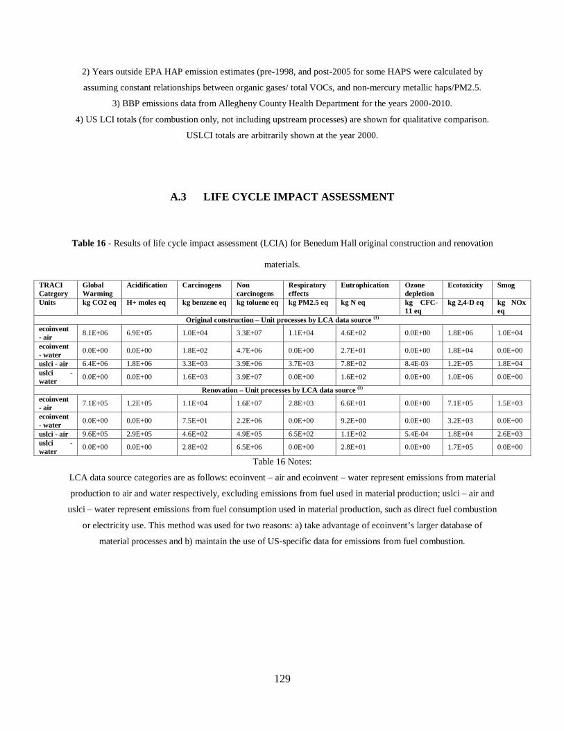
129
2) Years outside EPA HAP emission estimates (pre-1998, and post-2005 for some HAPS were calculated by
assuming constant relationships between organic gases/ total VOCs, and non-mercury metallic haps/PM2.5.
3) BBP emissions data from Allegheny County Health Department for the years 2000-2010.
4) US LCI totals (for combustion only, not including upstream processes) are shown for qualitative comparison.
USLCI totals are arbitrarily shown at the year 2000.
A.3 LIFE CYCLE IMPACT ASSESSMENT
Table 16 - Results of life cycle impact assessment (LCIA) for Benedum Hall original construction and renovation
materials.
TRACI Category
Global Warming
Acidification Carcinogens Non carcinogens
Respiratory effects
Eutrophication Ozone depletion
Ecotoxicity Smog
Units kg CO2 eq H+ moles eq kg benzene eq kg toluene eq kg PM2.5 eq kg N eq kg CFC-11 eq
kg 2,4-D eq kg NOx eq
Original construction – Unit processes by LCA data source (1) ecoinvent - air 8.1E+06 6.9E+05 1.0E+04 3.3E+07 1.1E+04 4.6E+02 0.0E+00 1.8E+06 1.0E+04
ecoinvent - water 0.0E+00 0.0E+00 1.8E+02 4.7E+06 0.0E+00 2.7E+01 0.0E+00 1.8E+04 0.0E+00
uslci - air 6.4E+06 1.8E+06 3.3E+03 3.9E+06 3.7E+03 7.8E+02 8.4E-03 1.2E+05 1.8E+04 uslci - water 0.0E+00 0.0E+00 1.6E+03 3.9E+07 0.0E+00 1.6E+02 0.0E+00 1.0E+06 0.0E+00
Renovation – Unit processes by LCA data source (1) ecoinvent - air 7.1E+05 1.2E+05 1.1E+04 1.6E+07 2.8E+03 6.6E+01 0.0E+00 7.1E+05 1.5E+03
ecoinvent - water 0.0E+00 0.0E+00 7.5E+01 2.2E+06 0.0E+00 9.2E+00 0.0E+00 3.2E+03 0.0E+00
uslci - air 9.6E+05 2.9E+05 4.6E+02 4.9E+05 6.5E+02 1.1E+02 5.4E-04 1.8E+04 2.6E+03 uslci - water 0.0E+00 0.0E+00 2.8E+02 6.5E+06 0.0E+00 2.8E+01 0.0E+00 1.7E+05 0.0E+00
Table 16 Notes:
LCA data source categories are as follows: ecoinvent – air and ecoinvent – water represent emissions from material
production to air and water respectively, excluding emissions from fuel used in material production; uslci – air and
uslci – water represent emissions from fuel consumption used in material production, such as direct fuel combustion
or electricity use. This method was used for two reasons: a) take advantage of ecoinvent’s larger database of
material processes and b) maintain the use of US-specific data for emissions from fuel combustion.

130
Figure 27 - Normalized TRACI results from Benedum Hall original construction materials showing percentage
contributions from unit processes.
Figure 28 - Normalized TRACI results from Benedum Hall renovation materials showing percentage contributions
from unit processes.

131
Figure 29 - (1 of 4) Time series of DLCA results for the sensitivity analysis, shown as cumulative percent
deviations from the baseline scenario for the remaining categories not shown in Figure 6.

132
Figure 29 - (2 of 4) Time series of DLCA results for the sensitivity analysis, shown as cumulative percent
deviations from the baseline scenario for the remaining categories not shown in Figure 6.

133
Figure 29 - (3 of 4) Time series of DLCA results for the sensitivity analysis, shown as cumulative percent
deviations from the baseline scenario for the remaining categories not shown in Figure 6.

134
Figure 29 - (4 of 4) Time series of DLCA results for the sensitivity analysis, shown as cumulative percent
deviations from the baseline scenario for the remaining categories not shown in Figure 6.

135
APPENDIX B
DATA COLLECTION FOR THE IN-DEPTH MCSI CASE STUDY
B.1 MCSI BUILDING DATA
B.1.1 Data collection and organization
A floor plan of the MCSI annex is shown in Figure 30 on the following page. Raw data and
model calculations from the study period are organized in a series of text (.csv) files and Excel
spreadsheets, as indicated in Table 17.

136
Figure 30 - Floor plan of the MCSI annex showing data collection points.

137
Table 17- Data organization and file structure

138
B.2 EXTERNAL REFERENCE DATA FOR IEQ MODEL
B.2.1 Allegheny County Health Department (ACHD) PM2.5
Figure 31 shows the correlation obtained from a linear least-squares fit of the ACHD hourly
particle mass monitoring data versus the hourly average outdoor particle count from this study.
The best-fit line shown in Figure 31 was applied to the hourly outdoor particle counts to generate
hourly PM2.5 outdoor mass estimates. The mass estimates were further multiplied by the ratio at
each hourly interval of the indoor particle count in each compartment to the outdoor particle
count, to generate indoor mass concentration estimates for each compartment. The indoor mass
concentration estimates were multiplied by the occupancy estimates and respiration rate in order
to estimate intake in each compartment at each interval.
Figure 31 - Linear regression of outdoor particle number from this study and particle mass from ACHD during the
study time period

139
B.2.2 VOC SPECIATION
Table 18 gives the master list of VOCs used in this study. It represents a compilation of all
VOCs listed in the ACHD, PAQS and BASE reference studies, along with parameters necessary
for conversion of TVOC readings to LCIA results: molecular weights, PID correction factors,
and USE-Tox effect factors, and calculated values for TVOC equivalents and toxicity potentials.
Outdoor Estimate - The average outdoor TVOC concentration from this study was 0.15
ppm, and the calculated value from the PAQS was also 0.15 ppm. From this comparison, we
assumed that the PAQS data were reasonably representative of the concentrations of outdoor
species during our study period. The majority of the estimated PID reading for the PAQS data
was comprised of butane and isobutane, two relatively nontoxic species. By contrast, the ACHD
report lists only hazardous air pollutants (HAPs), and does not include butane, isobutane or other
species not listed as HAPs by EPA. The total estimated PID reading for the ACHD data was
0.012 ppm, of which 92% was comprised of the compounds also found in the PAQS data, which
in turn was 95% of the estimated PID reading from the PAQS data for those compounds.
Given the strong similarities across individual compound concentrations between the
PAQS and ACHD data, we assumed that these data represented separate samples of a very
similar population of VOCs, with one sample (PAQS) focused on mass and one sample (ACHD)
focused on toxicity. We note that if one simply added the PID equivalents of the remaining
HAPs from ACHD to the PAQS total, the result would be the same to two significant digits.
Equation 34 was used to calculate the ambient outdoor air EFs for cancer and noncancer
effects based on the speciation of the ACHD data:

140
Equation 34
∑ ×=x
xACHDxPAQSTVOC
toaTVOCtoa EFCM
CCEF ,
,
,,
,
where EFoa,t is the estimated effect factor for cancer or noncancer effects for the outdoor
air in our study at time t, CTVOC,oa,t is the outdoor air TVOC reading at time t, CTVOC,PAQS is the
PID equivalent TVOC concentration for the PAQS (0.13 ppm), and CMx,ACHD is the mass
concentration of VOC species x from the ACHD data. With the time-averaged value CTVOC,oa
equal to CTVOC,PAQS, the average estimated values for EFoa for this study were 2.3 x 10⁻⁹ cases/m3
inhaled for cancer effects and 4.5 x 10⁻⁹ for noncancer effects. Over 99% of the cancer value was
due to formaldehyde, while 91% of the noncancer value was due to acrolein.
Indoor Estimate - We obtained the EPA BASE study raw data from the EPA’s Indoor
Environments Division. BASE study VOC sampling was conducted at 100 buildings with
typically 2 outdoor and 4 indoor time-integrated samples conducted at each site. A total of 80
VOCs (including formaldehyde and acetaldehyde, which are labeled aldehydes and not VOCs in
BASE study terminology) were analyzed, though not every building was tested for every VOC.
All 80 of these VOCs are listed in Table 18.
EPA provided a breakdown of indoor and outdoor VOC concentrations by 5-percentile
increments across the sample population (Min, 5th%, 10th%...95th%, Max) but did not report the
quantity [Indoor - Outdoor] for each site. Since indoor concentrations for most VOCs at most
sites were higher than outdoor concentrations, we computed the quantity [Average Indoor -
Average Outdoor] concentration for each VOC at each site. Equation 24 was then used to
estimate PID equivalent TVOC concentrations as ppm isobutylene for each site. The median PID
equivalent concentration for the BASE study was 0.027 ppm, whereas the measured average
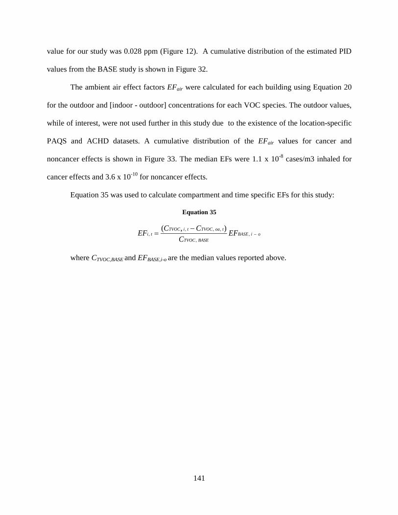
141
value for our study was 0.028 ppm (Figure 12). A cumulative distribution of the estimated PID
values from the BASE study is shown in Figure 32.
The ambient air effect factors EFair were calculated for each building using Equation 20
for the outdoor and [indoor - outdoor] concentrations for each VOC species. The outdoor values,
while of interest, were not used further in this study due to the existence of the location-specific
PAQS and ACHD datasets. A cumulative distribution of the EFair values for cancer and
noncancer effects is shown in Figure 33. The median EFs were 1.1 x 10⁻⁸ cases/m3 inhaled for
cancer effects and 3.6 x 10⁻¹⁰ for noncancer effects.
Equation 35 was used to calculate compartment and time specific EFs for this study:
Equation 35
oiBASEBASETVOC
toaTVOCtiTVOCti EF
CCCEF −
−= ,
,
,,,,
),(
where CTVOC,BASE and EFBASE,i-o are the median values reported above.

142
Figure 32 - Cumulative distribution of indoor - outdoor PID equivalent TVOC concentrations from EPA
BASE study
Figure 33 - Cumulative distribution of indoor - outdoor effect factors from EPA BASE study

Compound CAS Number Mol. Wt PID CorrectionUSE-Tox EF Cancer
USE-Tox EF Noncancer
CF Cancer Urban Air
CF Cancer Rural Air
CF Noncancer Urban Air
CF Noncancer Rural Air
Units-> g/molppm isobuylene (isobutylene)/ cases/kg inhaled cases/kg inhaled
cases/kg emitted
cases/kg emitted cases/kg emitted cases/kg emitted
1,1,1-Trichloroethane 71-55-6 133 Not detected 0.00E+00 1.08E-04 0.00E+00 0.00E+00 1.90E-08 1.64E-08
1,1,2,2-Tetrachloroethane 79-34-5 168 Not detected 5.33E-02 n/a 2.04E-06 7.50E-07 n/a n/a
1,1,2-Trichloro-1,2,2-trifluoroethane 76-13-1 187 Not detected 0.00E+00 1.14E-04 0.00E+00 0.00E+00 4.12E-07 4.09E-07
1,1,2-Trichloroethane 79-00-5 133 Not detected 3.71E-02 1.16E-01 1.52E-06 6.16E-07 4.73E-06 1.92E-06
1,1-Dichloroethane 75-34-3 99 Not listed 0.00E+00 n/a 0.00E+00 0.00E+00 n/a n/a
1,1-Dichloroethylene 75-35-4 97 0.82 5.90E-02 9.45E-03 1.47E-06 9.59E-08 2.36E-07 1.54E-08
1,2,4-Trichlorobenzene 120-82-1 181 0.46 n/a 8.59E-03 n/a n/a 3.43E-07 1.35E-07
1,2,4-Trimethylbenzene 95-63-6 120 Not listed 2.63E-04 n/a 5.89E-09 1.59E-10 n/a n/a
1,2-Dibromoethane 106-93-4 188 1.7 7.25E-01 4.71E-03 2.84E-05 1.08E-05 1.84E-07 7.01E-08
1,2-Dichloro-1,1,2,2-tetrafloroethane 76-14-2 171 Not listed Not listed Not listed Not listed Not listed Not listed Not listed
1,2-Dichlorobenzene 95-50-1 147 0.47 0.00E+00 1.48E-03 0.00E+00 0.00E+00 5.75E-08 2.16E-08
1,2-Dichloroethane 107-06-2 99 Not detected 1.42E-02 n/a 5.87E-07 2.43E-07 n/a n/a
1,2-Dichloropropane 78-87-5 113 0 7.39E-03 1.03E+00 2.82E-07 1.02E-07 3.92E-05 1.43E-05
1,3,5-Trimethylbenzene 108-67-8 120 0.35 n/a n/a n/a n/a n/a n/a
1,3-Butadiene 106-99-0 54 0.85 5.65E-02 8.45E-02 1.13E-06 1.66E-08 1.68E-06 2.49E-08
1,3-Dichlorobenzene 541-73-1 147 0 n/a n/a n/a n/a n/a n/a
1,4-Dichlorobenzene 106-46-7 147 Not listed 7.53E-03 2.23E-03 3.06E-07 1.24E-07 9.13E-08 3.72E-08
1-butanol 71-36-3 74 4.7 n/a 2.03E-03 n/a n/a 5.27E-08 5.03E-09
1-butene 106-98-9 56 0.9 Not listed Not listed Not listed Not listed Not listed Not listed
1-Ethyl-4-methylbenzene 622-96-8 120 Not listed Not listed Not listed Not listed Not listed Not listed Not listed
1-pentene 109-67-1 70 Not listed Not listed Not listed Not listed Not listed Not listed Not listed
2,2,4-trimethyl-1,3-pentanediol diisobutyrate 6846-50-0 286 Not listed Not listed Not listed Not listed Not listed Not listed Not listed
2,2,4-trimethyl-1,3-pentanediol monoisobutyrate 25265-77-4 216 Not listed n/a n/a n/a n/a n/a n/a
2-butoxyethanol 111-76-2 118 1.2 1.19E-03 7.92E-03 2.93E-08 2.49E-09 2.02E-07 2.40E-08
2-ethyl-1-hexanol 104-76-7 130 1.9 1.21E-03 n/a 3.07E-08 2.66E-09 n/a n/a
2-methyl-1-butene 563-46-2 70 Not listed Not listed Not listed Not listed Not listed Not listed Not listed
2-methyl-1-propanol 78-83-1 74 Not listed n/a 8.04E-04 n/a n/a 2.14E-08 2.45E-09
2-methylpropene 115-11-7 56 1 3.23E-04 n/a 6.75E-09 1.23E-10 n/a n/a
3-methyl-1-butene 563-45-1 70 Not listed Not listed Not listed Not listed Not listed Not listed Not listed
3-methylfuran 930-27-8 82 Not listed Not listed Not listed Not listed Not listed Not listed Not listed
4-phenylcyclohexene 4994-16-5 158 Not listed Not listed Not listed Not listed Not listed Not listed Not listed
Acetaldehyde 75-07-0 44 6 7.49E-03 3.85E-02 1.81E-07 9.18E-09 9.29E-07 4.71E-08
Acetone 67-64-1 58 1.1 n/a 2.82E-04 n/a n/a 9.67E-09 2.83E-09
Acetonitrile 75-05-8 41 Not detected 0.00E+00 2.79E-03 0.00E+00 0.00E+00 9.72E-08 2.96E-08
Acrolein 107-02-8 56 3.9 0.00E+00 5.97E+01 0.00E+00 0.00E+00 1.41E-03 5.56E-05
Acrylonitrile 107-13-1 53 Not detected 1.28E-01 3.52E-01 3.54E-06 4.89E-07 9.68E-06 1.27E-06
a-pinene 80-56-8 136 0.31 n/a n/a n/a n/a n/a n/a
Benzene 71-43-2 78 0.53 1.47E-02 3.72E-03 4.74E-07 1.20E-07 1.20E-07 3.04E-08
Benzyl chloride 100-44-7 127 0.6 3.32E-02 n/a 9.52E-07 1.56E-07 n/a n/a
Bromodichloromethane 75-27-4 164 Not listed 4.28E-02 5.05E-02 2.23E-06 1.20E-06 2.64E-06 1.41E-06
Bromoform 75-25-2 253 2.5 1.77E-03 1.42E-02 7.80E-08 3.51E-08 6.26E-07 2.82E-07
Bromomethane 74-83-9 95 1.7 0.00E+00 1.51E+00 0.00E+00 0.00E+00 1.14E-04 7.72E-05
Butanal 123-72-8 72 1.8 n/a n/a n/a n/a n/a n/a
Butane 106-97-8 58 67 Not listed Not listed Not listed Not listed Not listed Not listed
Butyl acetate 123-86-4 116 2.6 n/a n/a n/a n/a n/a n/a
Butylated hydroxytoluene 128-37-0 220 Not listed 3.13E-03 n/a 7.83E-08 7.37E-09 n/a n/a
c-2-butene 107-01-7 56 Not listed Not listed Not listed Not listed Not listed Not listed Not listed
Carbon disulfide 75-15-0 76 1.2 n/a 2.64E-01 n/a n/a 5.31E-05 4.67E-05
Carbon tetrachloride 56-23-5 154 Not detected 1.08E-01 3.58E-01 4.80E-05 4.54E-05 1.59E-04 1.50E-04
Chlorobenzene 108-90-7 113 0.4 4.64E-03 4.81E-03 1.61E-07 4.89E-08 1.67E-07 5.06E-08
Chloroethane 75-00-3 65 Not detected 1.13E-03 4.18E-05 4.42E-08 1.68E-08 1.64E-09 6.25E-10
Chloroethene 75-01-4 63 2 1.93E-01 6.69E-02 5.03E-06 4.63E-07 1.74E-06 1.61E-07
Chloroform 67-66-3 119 Not detected 5.64E-03 3.25E-02 2.99E-07 1.62E-07 1.71E-06 9.27E-07
Chloromethane 74-87-3 50 Not detected n/a 8.84E-03 n/a n/a 6.56E-07 4.41E-07
cis-1,2-dichloroethene 156-59-2 97 0.8 Not listed Not listed Not listed Not listed Not listed Not listed
cis-1,2-Dichloroethene 540-59-0 97 0.8 n/a n/a n/a n/a n/a n/a
cis-1,3-Dichloro-1-propene 52-75-6 111 0.96 Not listed Not listed Not listed Not listed Not listed Not listed
cis-1,3-dichloropropene 10061-01-5 111 Not listed n/a n/a n/a n/a n/a n/a
Cyclohexane 110-82-7 84 1.4 n/a 8.26E-04 n/a n/a 2.14E-08 1.86E-09
Use-Tox Effect and Characterization Factors

Compound CAS Number Mol. Wt PID CorrectionUSE-Tox EF Cancer
USE-Tox EF Noncancer
CF Cancer Urban Air
CF Cancer Rural Air
CF Noncancer Urban Air
CF Noncancer Rural Air
Units-> g/molppm isobuylene (isobutylene)/ cases/kg inhaled cases/kg inhaled
cases/kg emitted
cases/kg emitted cases/kg emitted cases/kg emitted
Use-Tox Effect and Characterization Factors
Cyclopentane 287-92-3 70 15 n/a n/a n/a n/a n/a n/a
Cyclopentene 142-29-0 68 Not listed Not listed Not listed Not listed Not listed Not listed Not listed
Dibrochloromethane 124-48-1 208 5.3 1.47E-02 1.19E-02 6.72E-07 3.16E-07 5.44E-07 2.55E-07
Dichlorodifluoromethane 75-71-8 121 Not detected 0.00E+00 8.47E-03 0.00E+00 0.00E+00 2.32E-05 2.30E-05
dimethy disulfide 624-92-0 94 0.2 Not listed Not listed Not listed Not listed Not listed Not listed
Dimethylsulfide 75-18-3 62 0.44 n/a n/a n/a n/a n/a n/a
d-limonene 5989-27-5 136 0.33 5.62E-03 n/a 8.59E-08 6.68E-10 n/a n/a
Ethanol 64-17-5 46 10 1.26E-04 n/a 3.64E-09 6.38E-10 n/a n/a
Ethyl acetate 141-78-6 88 4.6 n/a 2.82E-04 n/a n/a 8.63E-09 1.82E-09
Ethylbenzene 100-41-4 106 0.52 2.36E-02 3.85E-04 6.13E-07 5.55E-08 1.01E-08 9.44E-10
Formaldehyde 50-00-0 30 Not detected 1.06E+00 8.47E-03 2.54E-05 1.39E-06 2.67E-07 7.54E-08
Heptane 142-82-5 100 2.8 n/a n/a n/a n/a n/a n/a
Hexachloro-1,3-butadiene 87-68-3 261 Not listed 1.74E-02 n/a 2.10E-06 1.68E-06 n/a n/a
Hexanal 66-25-1 100 Not listed n/a n/a n/a n/a n/a n/a
Hexane 110-54-3 86 4.3 6.74E-05 9.16E-03 1.79E-09 1.93E-10 2.44E-07 2.62E-08
Isobutane 75-28-5 58 100 Not listed Not listed Not listed Not listed Not listed Not listed
Isopentane 78-78-4 72 8.2 Not listed Not listed Not listed Not listed Not listed Not listed
Isoprene 78-79-5 68 0.63 7.45E-03 n/a 1.35E-07 1.46E-09 n/a n/a
Isopropyl alcohol 67-63-0 60 6 0.00E+00 n/a 0.00E+00 0.00E+00 n/a n/a
m & p- Xylene 1330-20-7 106 0.44 Not listed Not listed Not listed Not listed Not listed Not listed
Methacrolein 78-85-3 70 Not listed Not listed Not listed Not listed Not listed Not listed Not listed
Methanol 67-56-1 32 Not detected n/a 5.08E-04 n/a n/a 1.63E-08 4.13E-09
Methyl butyl ketone 591-78-6 100 Not listed n/a n/a n/a n/a n/a n/a
Methyl ethyl ketone 78-93-3 72 0.9 n/a 3.02E-05 n/a n/a 1.27E-09 5.38E-10
Methyl isobutyl ketone 108-10-1 100 0.8 n/a 1.63E-04 n/a n/a 3.98E-09 2.16E-10
Methyl tert-butyl ether 1634-04-4 88 0.9 3.86E-03 6.46E-04 1.10E-07 1.77E-08 1.85E-08 2.99E-09
Methylene chloride 75-09-2 85 Not detected 1.86E-03 2.17E-02 8.92E-08 4.42E-08 1.04E-06 5.16E-07
Methylpentanes 96-14-0 86 Not listed Not listed Not listed Not listed Not listed Not listed Not listed
Methylvinylketone 78-94-4 70 Not listed n/a n/a n/a n/a n/a n/a
naphthalene 91-20-3 128 0.42 5.19E-02 7.19E-02 1.22E-06 5.15E-08 1.68E-06 6.40E-08
n-decane 124-18-5 142 1.4 n/a n/a n/a n/a n/a n/a
n-dodecane 112-40-3 170 Not listed Not listed Not listed Not listed Not listed Not listed Not listed
n-heptanal 111-71-7 114 Not listed Not listed Not listed Not listed Not listed Not listed Not listed
n-nonanal 124-19-6 142 Not listed Not listed Not listed Not listed Not listed Not listed Not listed
n-octane 111-65-9 114 1.8 n/a n/a n/a n/a n/a n/a
nonane 111-84-2 128 1.4 Not listed Not listed Not listed Not listed Not listed Not listed
n-undecane 1120-21-4 156 2 Not listed Not listed Not listed Not listed Not listed Not listed
o-xylene 95-47-6 106 0.46 n/a n/a n/a n/a n/a n/a
o-Xylene 1330-20-7 106 0.46 Not listed Not listed Not listed Not listed Not listed Not listed
Pentanal 110-62-3 86 Not listed n/a n/a n/a n/a n/a n/a
Pentane 109-66-0 72 8.4 n/a n/a n/a n/a n/a n/a
phenol 108-95-2 94 1 0.00E+00 3.29E-03 0.00E+00 0.00E+00 8.41E-08 1.32E-08Propane 74-98-6 44 Not detected Not listed Not listed Not listed Not listed Not listed Not listedPropene 115-07-1 42 1.4 0.00E+00 n/a 0.00E+00 0.00E+00 n/a n/a
Propionaldehyde 123-38-6 58 1.9 n/a n/a n/a n/a n/a n/a
Propyne 74-99-7 40 Not listed Not listed Not listed Not listed Not listed Not listed Not listed
Styrene 100-42-5 104 0.4 4.92E-02 9.84E-03 1.01E-06 1.66E-08 2.01E-07 3.32E-09
t-2-pentene 646-04-8 70 Not listed Not listed Not listed Not listed Not listed Not listed Not listed
Tetrachloroethylene 127-18-4 165 0.57 8.50E-03 3.23E-02 4.29E-07 2.23E-07 1.62E-06 8.40E-07
Tetrahydrofuran 109-99-9 72 1.7 2.82E-03 n/a 6.79E-08 3.39E-09 n/a n/a
Toluene 108-88-3 92 0.5 0.00E+00 3.64E-03 3.17E-12 3.18E-12 9.62E-08 9.90E-09
trans-1,3-dichloropropene 10061-02-6 111 Not listed Not listed Not listed Not listed Not listed Not listed Not listed
Trichloroethylene 79-01-6 131 0.54 1.72E-03 n/a 5.06E-08 9.36E-09 n/a n/a
Trichlorofluoromethane 75-69-4 137 Not listed 0.00E+00 1.46E-03 0.00E+00 0.00E+00 1.81E-06 1.77E-06
TOTALS

Compound CAS Number
Units->
1,1,1-Trichloroethane 71-55-6
1,1,2,2-Tetrachloroethane 79-34-5
1,1,2-Trichloro-1,2,2-trifluoroethane 76-13-1
1,1,2-Trichloroethane 79-00-5
1,1-Dichloroethane 75-34-3
1,1-Dichloroethylene 75-35-4
1,2,4-Trichlorobenzene 120-82-1
1,2,4-Trimethylbenzene 95-63-6
1,2-Dibromoethane 106-93-4
1,2-Dichloro-1,1,2,2-tetrafloroethane 76-14-2
1,2-Dichlorobenzene 95-50-1
1,2-Dichloroethane 107-06-2
1,2-Dichloropropane 78-87-5
1,3,5-Trimethylbenzene 108-67-8
1,3-Butadiene 106-99-0
1,3-Dichlorobenzene 541-73-1
1,4-Dichlorobenzene 106-46-7
1-butanol 71-36-3
1-butene 106-98-9
1-Ethyl-4-methylbenzene 622-96-8
1-pentene 109-67-1
2,2,4-trimethyl-1,3-pentanediol diisobutyrate 6846-50-0
2,2,4-trimethyl-1,3-pentanediol monoisobutyrate 25265-77-4
2-butoxyethanol 111-76-2
2-ethyl-1-hexanol 104-76-7
2-methyl-1-butene 563-46-2
2-methyl-1-propanol 78-83-1
2-methylpropene 115-11-7
3-methyl-1-butene 563-45-1
3-methylfuran 930-27-8
4-phenylcyclohexene 4994-16-5
Acetaldehyde 75-07-0
Acetone 67-64-1
Acetonitrile 75-05-8
Acrolein 107-02-8
Acrylonitrile 107-13-1
a-pinene 80-56-8
Benzene 71-43-2
Benzyl chloride 100-44-7
Bromodichloromethane 75-27-4
Bromoform 75-25-2
Bromomethane 74-83-9
Butanal 123-72-8
Butane 106-97-8
Butyl acetate 123-86-4
Butylated hydroxytoluene 128-37-0
c-2-butene 107-01-7
Carbon disulfide 75-15-0
Carbon tetrachloride 56-23-5
Chlorobenzene 108-90-7
Chloroethane 75-00-3
Chloroethene 75-01-4
Chloroform 67-66-3
Chloromethane 74-87-3
cis-1,2-dichloroethene 156-59-2
cis-1,2-Dichloroethene 540-59-0
cis-1,3-Dichloro-1-propene 52-75-6
cis-1,3-dichloropropene 10061-01-5
Cyclohexane 110-82-7
Median, ppt IQR, d ppt Median, ppt IQR,d
Not listed Not listed Not listed Not listed 0 0.00E+00 0.0% 0.000 0.00E+00 0.00E+00
Not listed Not listed Not listed Not listed 0 0.00E+00 0.0% 0.000 0.00E+00 0.00E+00
Not listed Not listed Not listed Not listed 0 0.00E+00 0.0% 0.000 0.00E+00 0.00E+00
Not listed Not listed Not listed Not listed 0 0.00E+00 0.0% 0.000 0.00E+00 0.00E+00
Not listed Not listed Not listed Not listed 0 0.00E+00 0.0% 0.000 0.00E+00 0.00E+00
Not listed Not listed Not listed Not listed 0 0.00E+00 0.0% 0.000 0.00E+00 0.00E+00
Not listed Not listed Not listed Not listed 0 0.00E+00 0.0% 0.000 0.00E+00 0.00E+00
Not listed Not listed Not listed Not listed 0 0.00E+00 0.0% 0.000 0.00E+00 0.00E+00
Not listed Not listed Not listed Not listed 0 0.00E+00 0.0% 0.000 0.00E+00 0.00E+00
Not listed Not listed Not listed Not listed 0 0.00E+00 0.0% 0.000 0.00E+00 0.00E+00
Not listed Not listed Not listed Not listed 0 0.00E+00 0.0% 0.000 0.00E+00 0.00E+00
Not listed Not listed Not listed Not listed 0 0.00E+00 0.0% 0.000 0.00E+00 0.00E+00
Not listed Not listed Not listed Not listed 0 0.00E+00 0.0% 0.000 0.00E+00 0.00E+00
Not listed Not listed Not listed Not listed 0 0.00E+00 0.0% 0.000 0.00E+00 0.00E+00
Not listed Not listed Not listed Not listed 0 0.00E+00 0.0% 0.000 0.00E+00 0.00E+00
Not listed Not listed Not listed Not listed 0 0.00E+00 0.0% 0.000 0.00E+00 0.00E+00
Not listed Not listed Not listed Not listed 0 0.00E+00 0.0% 0.000 0.00E+00 0.00E+00
Not listed Not listed Not listed Not listed 0 0.00E+00 0.0% 0.000 0.00E+00 0.00E+00
57 40 – 83 62 44 – 88 59.5 5.36E-05 0.0% 0.136 0.00E+00 0.00E+00
Not listed Not listed Not listed Not listed 0 0.00E+00 0.0% 0.000 0.00E+00 0.00E+00
36 24 – 56 20 14 – 32 28 0.00E+00 0.0% 0.080 0.00E+00 0.00E+00
Not listed Not listed Not listed Not listed 0 0.00E+00 0.0% 0.000 0.00E+00 0.00E+00
Not listed Not listed Not listed Not listed 0 0.00E+00 0.0% 0.000 0.00E+00 0.00E+00
Not listed Not listed Not listed Not listed 0 0.00E+00 0.0% 0.000 0.00E+00 0.00E+00
Not listed Not listed Not listed Not listed 0 0.00E+00 0.0% 0.000 0.00E+00 0.00E+00
16 11 – 25 42 22 – 74 29 0.00E+00 0.0% 0.083 0.00E+00 0.00E+00
Not listed Not listed Not listed Not listed 0 0.00E+00 0.0% 0.000 0.00E+00 0.00E+00
38 32 – 51 NQf NQf 38 3.80E-05 0.0% 0.087 2.81E-14 0.00E+00
6 5 – 10 19 12 – 35 12.5 0.00E+00 0.0% 0.036 0.00E+00 0.00E+00
<DLg <DLg 10 6 – 16 10 0.00E+00 0.0% 0.034 0.00E+00 0.00E+00
Not listed Not listed Not listed Not listed 0 0.00E+00 0.0% 0.000 0.00E+00 0.00E+00
538 403 – 729 1559 1103 – 2150 1048.5 6.29E-03 4.2% 1.887 1.41E-11 7.26E-11
943 655 – 1385 4031 3128 – 4894 2487 2.74E-03 1.8% 5.900 0.00E+00 1.67E-12
NQf NQf 131 105 – 155 131 0.00E+00 0.0% 0.220 0.00E+00 6.12E-13
Not listed Not listed Not listed Not listed 0 0.00E+00 0.0% 0.000 0.00E+00 0.00E+00
Not listed Not listed Not listed Not listed 0 0.00E+00 0.0% 0.000 0.00E+00 0.00E+00
<DLg <DLg 16 10 – 29 16 4.96E-06 0.0% 0.089 0.00E+00 0.00E+00
279 231 – 355 215 143 – 405 247 1.31E-04 0.1% 0.788 1.16E-11 2.93E-12
Not listed Not listed Not listed Not listed 0 0.00E+00 0.0% 0.000 0.00E+00 0.00E+00
Not listed Not listed Not listed Not listed 0 0.00E+00 0.0% 0.000 0.00E+00 0.00E+00
Not listed Not listed Not listed Not listed 0 0.00E+00 0.0% 0.000 0.00E+00 0.00E+00
Not listed Not listed Not listed Not listed 0 0.00E+00 0.0% 0.000 0.00E+00 0.00E+00
NQf NQf 91 64 – 122 91 1.64E-04 0.1% 0.268 0.00E+00 0.00E+00
1333 978 – 1799 632 375 – 1106 982.5 6.58E-02 43.8% 2.331 0.00E+00 0.00E+00
Not listed Not listed Not listed Not listed 0 0.00E+00 0.0% 0.000 0.00E+00 0.00E+00
Not listed Not listed Not listed Not listed 0 0.00E+00 0.0% 0.000 0.00E+00 0.00E+00
27 18 – 44 20 15 – 28 23.5 0.00E+00 0.0% 0.054 0.00E+00 0.00E+00
Not listed Not listed Not listed Not listed 0 0.00E+00 0.0% 0.000 0.00E+00 0.00E+00
Not listed Not listed Not listed Not listed 0 0.00E+00 0.0% 0.000 0.00E+00 0.00E+00
Not listed Not listed Not listed Not listed 0 0.00E+00 0.0% 0.000 0.00E+00 0.00E+00
Not listed Not listed Not listed Not listed 0 0.00E+00 0.0% 0.000 0.00E+00 0.00E+00
Not listed Not listed Not listed Not listed 0 0.00E+00 0.0% 0.000 0.00E+00 0.00E+00
11 10 – 13 17 13 – 30 14 0.00E+00 0.0% 0.068 3.84E-13 2.21E-12
Not listed Not listed Not listed Not listed 0 0.00E+00 0.0% 0.000 0.00E+00 0.00E+00
Not listed Not listed Not listed Not listed 0 0.00E+00 0.0% 0.000 0.00E+00 0.00E+00
Not listed Not listed Not listed Not listed 0 0.00E+00 0.0% 0.000 0.00E+00 0.00E+00
Not listed Not listed Not listed Not listed 0 0.00E+00 0.0% 0.000 0.00E+00 0.00E+00
Not listed Not listed Not listed Not listed 0 0.00E+00 0.0% 0.000 0.00E+00 0.00E+00
Not listed Not listed Not listed Not listed 0 0.00E+00 0.0% 0.000 0.00E+00 0.00E+00
Summer WinterAnnual Median
Concentration, ppt
PID Equivalent Concentration,
ppm isobutylene
PAQS (Millet et al) data and calculationsAnnual Median
Mass concentration
µg/m3
Noncancer toxicity potential
(Cases/m3 air inhaled)
Cancer toxicity potential
(Cases/m3 air inhaled)
% Total PID Value

Compound CAS Number
Units->
Cyclopentane 287-92-3
Cyclopentene 142-29-0
Dibrochloromethane 124-48-1
Dichlorodifluoromethane 75-71-8
dimethy disulfide 624-92-0
Dimethylsulfide 75-18-3
d-limonene 5989-27-5
Ethanol 64-17-5
Ethyl acetate 141-78-6
Ethylbenzene 100-41-4
Formaldehyde 50-00-0
Heptane 142-82-5
Hexachloro-1,3-butadiene 87-68-3
Hexanal 66-25-1
Hexane 110-54-3
Isobutane 75-28-5
Isopentane 78-78-4
Isoprene 78-79-5
Isopropyl alcohol 67-63-0
m & p- Xylene 1330-20-7
Methacrolein 78-85-3
Methanol 67-56-1
Methyl butyl ketone 591-78-6
Methyl ethyl ketone 78-93-3
Methyl isobutyl ketone 108-10-1
Methyl tert-butyl ether 1634-04-4
Methylene chloride 75-09-2
Methylpentanes 96-14-0
Methylvinylketone 78-94-4
naphthalene 91-20-3
n-decane 124-18-5
n-dodecane 112-40-3
n-heptanal 111-71-7
n-nonanal 124-19-6
n-octane 111-65-9
nonane 111-84-2
n-undecane 1120-21-4
o-xylene 95-47-6
o-Xylene 1330-20-7
Pentanal 110-62-3
Pentane 109-66-0
phenol 108-95-2Propane 74-98-6Propene 115-07-1
Propionaldehyde 123-38-6
Propyne 74-99-7
Styrene 100-42-5
t-2-pentene 646-04-8
Tetrachloroethylene 127-18-4
Tetrahydrofuran 109-99-9
Toluene 108-88-3
trans-1,3-dichloropropene 10061-02-6
Trichloroethylene 79-01-6
Trichlorofluoromethane 75-69-4
TOTALS
Median, ppt IQR, d ppt Median, ppt IQR,d
Summer WinterAnnual Median
Concentration, ppt
PID Equivalent Concentration,
ppm isobutylene
PAQS (Millet et al) data and calculationsAnnual Median
Mass concentration
µg/m3
Noncancer toxicity potential
(Cases/m3 air inhaled)
Cancer toxicity potential
(Cases/m3 air inhaled)
% Total PID Value
53 35 – 92 47 36 – 72 50 7.50E-04 0.5% 0.143 0.00E+00 0.00E+00
NQf NQf 3 0 – 8 3 0.00E+00 0.0% 0.008 0.00E+00 0.00E+00
Not listed Not listed Not listed Not listed 0 0.00E+00 0.0% 0.000 0.00E+00 0.00E+00
Not listed Not listed Not listed Not listed 0 0.00E+00 0.0% 0.000 0.00E+00 0.00E+00
Not listed Not listed Not listed Not listed 0 0.00E+00 0.0% 0.000 0.00E+00 0.00E+00
NQf NQf 7 5 – 10 7 3.08E-06 0.0% 0.018 0.00E+00 0.00E+00
Not listed Not listed Not listed Not listed 0 0.00E+00 0.0% 0.000 0.00E+00 0.00E+00
989 673 – 1416 1722 1017 – 3567 1355.5 1.36E-02 9.0% 2.550 3.21E-13 0.00E+00
Not listed Not listed Not listed Not listed 0 0.00E+00 0.0% 0.000 0.00E+00 0.00E+00
47 34 – 69 71 44 – 141 59 3.07E-05 0.0% 0.256 6.03E-12 9.86E-14
Not listed Not listed Not listed Not listed 0 0.00E+00 0.0% 0.000 0.00E+00 0.00E+00
Not listed Not listed Not listed Not listed 0 0.00E+00 0.0% 0.000 0.00E+00 0.00E+00
Not listed Not listed Not listed Not listed 0 0.00E+00 0.0% 0.000 0.00E+00 0.00E+00
34 22 – 52 NQf NQf 34 0.00E+00 0.0% 0.139 0.00E+00 0.00E+00
147 116 – 199 129 81 – 231 138 5.93E-04 0.4% 0.485 3.27E-14 4.45E-12
668 479 – 953 323 212 – 634 495.5 4.96E-02 33.0% 1.175 0.00E+00 0.00E+00
575 448 – 809 649 409 – 1139 612 5.02E-03 3.3% 1.802 0.00E+00 0.00E+00
<DLg <DLg 619 153 – 1475 619 3.90E-04 0.3% 1.722 1.28E-11 0.00E+00
131 86 – 199 235 147 – 432 183 1.10E-03 0.7% 0.449 0.00E+00 0.00E+00
113 76 – 176 163 89 – 306 138 6.07E-05 0.0% 0.598 0.00E+00 0.00E+00
<DLg <DLg 266 178 – 366 266 0.00E+00 0.0% 0.762 0.00E+00 0.00E+00
3760 2347 – 5773 10717 7122 – 14601 7238.5 0.00E+00 0.0% 9.474 0.00E+00 4.82E-12
Not listed Not listed Not listed Not listed 0 0.00E+00 0.0% 0.000 0.00E+00 0.00E+00
215 153 – 299 559 408 – 674 387 3.48E-04 0.2% 1.140 0.00E+00 3.44E-14
Not listed Not listed Not listed Not listed 0 0.00E+00 0.0% 0.000 0.00E+00 0.00E+00
10 7 – 14 31 19 – 61 20.5 1.85E-05 0.0% 0.074 2.85E-13 4.76E-14
NQf NQf 79 48 – 145 79 0.00E+00 0.0% 0.275 5.10E-13 5.97E-12
268 203 – 368 276 183 – 506 272 0.00E+00 0.0% 0.957 0.00E+00 0.00E+00
<DLg <DLg 463 273 – 665 463 0.00E+00 0.0% 1.326 0.00E+00 0.00E+00
Not listed Not listed Not listed Not listed 0 0.00E+00 0.0% 0.000 0.00E+00 0.00E+00
Not listed Not listed Not listed Not listed 0 0.00E+00 0.0% 0.000 0.00E+00 0.00E+00
Not listed Not listed Not listed Not listed 0 0.00E+00 0.0% 0.000 0.00E+00 0.00E+00
Not listed Not listed Not listed Not listed 0 0.00E+00 0.0% 0.000 0.00E+00 0.00E+00
Not listed Not listed Not listed Not listed 0 0.00E+00 0.0% 0.000 0.00E+00 0.00E+00
Not listed Not listed Not listed Not listed 0 0.00E+00 0.0% 0.000 0.00E+00 0.00E+00
Not listed Not listed Not listed Not listed 0 0.00E+00 0.0% 0.000 0.00E+00 0.00E+00
Not listed Not listed Not listed Not listed 0 0.00E+00 0.0% 0.000 0.00E+00 0.00E+00
Not listed Not listed Not listed Not listed 0 0.00E+00 0.0% 0.000 0.00E+00 0.00E+00
60 41 – 89 52 29 – 93 56 2.58E-05 0.0% 0.243 0.00E+00 0.00E+00
NQf NQf 137 98 – 193 137 0.00E+00 0.0% 0.482 0.00E+00 0.00E+00
355 279 – 493 352 213 – 613 353.5 2.97E-03 2.0% 1.041 0.00E+00 0.00E+00
Not listed Not listed Not listed Not listed 0 0.00E+00 0.0% 0.000 0.00E+00 0.00E+002960 2087 – 4307 1787 992 – 3540 2373.5 0.00E+00 0.0% 4.271 0.00E+00 0.00E+00214 147 – 306 219 159 – 336 216.5 3.03E-04 0.2% 0.372 0.00E+00 0.00E+00
Not listed Not listed Not listed Not listed 0 0.00E+00 0.0% 0.000 0.00E+00 0.00E+00
29 22 – 40 7 5 – 12 18 0.00E+00 0.0% 0.029 0.00E+00 0.00E+00
Not listed Not listed Not listed Not listed 0 0.00E+00 0.0% 0.000 0.00E+00 0.00E+00
19 12 – 33 44 33 – 62 31.5 0.00E+00 0.0% 0.090 0.00E+00 0.00E+00
18 12 – 25 22 13 – 41 20 1.14E-05 0.0% 0.135 1.15E-12 4.36E-12
Not listed Not listed Not listed Not listed 0 0.00E+00 0.0% 0.000 0.00E+00 0.00E+00
331 248 – 494 443 274 – 902 387 1.94E-04 0.1% 1.456 0.00E+00 5.29E-12
Not listed Not listed Not listed Not listed 0 0.00E+00 0.0% 0.000 0.00E+00 0.00E+00
Not listed Not listed Not listed Not listed 0 0.00E+00 0.0% 0.000 0.00E+00 0.00E+00
Not listed Not listed Not listed Not listed 0 0.00E+00 0.0% 0.000 0.00E+00 0.00E+00
0.150 100% 43.53 4.73E-11 1.05E-10

Compound CAS Number
Units->
1,1,1-Trichloroethane 71-55-6
1,1,2,2-Tetrachloroethane 79-34-5
1,1,2-Trichloro-1,2,2-trifluoroethane 76-13-1
1,1,2-Trichloroethane 79-00-5
1,1-Dichloroethane 75-34-3
1,1-Dichloroethylene 75-35-4
1,2,4-Trichlorobenzene 120-82-1
1,2,4-Trimethylbenzene 95-63-6
1,2-Dibromoethane 106-93-4
1,2-Dichloro-1,1,2,2-tetrafloroethane 76-14-2
1,2-Dichlorobenzene 95-50-1
1,2-Dichloroethane 107-06-2
1,2-Dichloropropane 78-87-5
1,3,5-Trimethylbenzene 108-67-8
1,3-Butadiene 106-99-0
1,3-Dichlorobenzene 541-73-1
1,4-Dichlorobenzene 106-46-7
1-butanol 71-36-3
1-butene 106-98-9
1-Ethyl-4-methylbenzene 622-96-8
1-pentene 109-67-1
2,2,4-trimethyl-1,3-pentanediol diisobutyrate 6846-50-0
2,2,4-trimethyl-1,3-pentanediol monoisobutyrate 25265-77-4
2-butoxyethanol 111-76-2
2-ethyl-1-hexanol 104-76-7
2-methyl-1-butene 563-46-2
2-methyl-1-propanol 78-83-1
2-methylpropene 115-11-7
3-methyl-1-butene 563-45-1
3-methylfuran 930-27-8
4-phenylcyclohexene 4994-16-5
Acetaldehyde 75-07-0
Acetone 67-64-1
Acetonitrile 75-05-8
Acrolein 107-02-8
Acrylonitrile 107-13-1
a-pinene 80-56-8
Benzene 71-43-2
Benzyl chloride 100-44-7
Bromodichloromethane 75-27-4
Bromoform 75-25-2
Bromomethane 74-83-9
Butanal 123-72-8
Butane 106-97-8
Butyl acetate 123-86-4
Butylated hydroxytoluene 128-37-0
c-2-butene 107-01-7
Carbon disulfide 75-15-0
Carbon tetrachloride 56-23-5
Chlorobenzene 108-90-7
Chloroethane 75-00-3
Chloroethene 75-01-4
Chloroform 67-66-3
Chloromethane 74-87-3
cis-1,2-dichloroethene 156-59-2
cis-1,2-Dichloroethene 540-59-0
cis-1,3-Dichloro-1-propene 52-75-6
cis-1,3-dichloropropene 10061-01-5
Cyclohexane 110-82-7
2009 2009 2010 2010
Average (ppb)24-Hour Maximum (ppb) Average (ppb)
24-Hour Maximum (ppb)
0.02 0.08 0.02 0.03 0.02 0.00E+00 0.0% 0.109 0.00E+00 1.17E-14
0 0.01 0 0.01 0 0.00E+00 0.0% 0.000 0.00E+00 0.00E+00
0.13 0.25 0.1 0.14 0.115 0.00E+00 0.0% 0.880 0.00E+00 1.00E-13
0 0.01 0 0.01 0 0.00E+00 0.0% 0.000 0.00E+00 0.00E+00
0 0.01 0 0.01 0 0.00E+00 0.0% 0.000 0.00E+00 0.00E+00
0 0.01 0 0.01 0 0.00E+00 0.0% 0.000 0.00E+00 0.00E+00
0.01 0.01 0 0.01 0.005 2.30E-06 0.0% 0.037 0.00E+00 3.18E-13
0.07 0.45 0.06 0.28 0.065 0.00E+00 0.0% 0.319 8.41E-14 0.00E+00
0 0.01 0 0.01 0 0.00E+00 0.0% 0.000 0.00E+00 0.00E+00
0.02 0.03 0.02 0.03 0.02 0.00E+00 0.0% 0.140 0.00E+00 0.00E+00
0 0.02 0 0.01 0 0.00E+00 0.0% 0.000 0.00E+00 0.00E+00
0.02 0.03 0.02 0.04 0.02 0.00E+00 0.0% 0.081 1.15E-12 0.00E+00
0 0.02 0.01 0.02 0.005 0.00E+00 0.0% 0.023 1.71E-13 2.38E-11
0.02 0.12 0.02 0.06 0.02 7.00E-06 0.1% 0.098 0.00E+00 0.00E+00
0.06 0.32 0.06 0.2 0.06 5.10E-05 0.4% 0.133 7.48E-12 1.12E-11
0 0.01 0 0.01 0 0.00E+00 0.0% 0.000 0.00E+00 0.00E+00
0.06 0.27 0.07 0.2 0.065 0.00E+00 0.0% 0.391 2.94E-12 8.72E-13
Not listed Not listed Not listed Not listed 0 0.00E+00 0.0% 0.000 0.00E+00 0.00E+00
0 0 0 0 0 0.00E+00 0.0% 0.000 0.00E+00 0.00E+00
0.02 0.13 0.02 0.18 0.02 0.00E+00 0.0% 0.098 0.00E+00 0.00E+00
0 0 0 0 0 0.00E+00 0.0% 0.000 0.00E+00 0.00E+00
Not listed Not listed Not listed Not listed 0 0.00E+00 0.0% 0.000 0.00E+00 0.00E+00
Not listed Not listed Not listed Not listed 0 0.00E+00 0.0% 0.000 0.00E+00 0.00E+00
0 0 0 0 0 0.00E+00 0.0% 0.000 0.00E+00 0.00E+00
0 0 0 0 0 0.00E+00 0.0% 0.000 0.00E+00 0.00E+00
0 0 0 0 0 0.00E+00 0.0% 0.000 0.00E+00 0.00E+00
Not listed Not listed Not listed Not listed 0 0.00E+00 0.0% 0.000 0.00E+00 0.00E+00
0 0 0 0 0 0.00E+00 0.0% 0.000 0.00E+00 0.00E+00
0 0 0 0 0 0.00E+00 0.0% 0.000 0.00E+00 0.00E+00
0 0 0 0 0 0.00E+00 0.0% 0.000 0.00E+00 0.00E+00
Not listed Not listed Not listed Not listed 0 0.00E+00 0.0% 0.000 0.00E+00 0.00E+00
0.78 1.63 0.9 1.84 0.84 5.04E-03 42.3% 1.512 1.13E-11 5.81E-11
1.93 5.58 1.86 4.68 1.895 2.08E-03 17.5% 4.495 0.00E+00 1.27E-12
0.14 0.28 0.3 0.75 0.22 0.00E+00 0.0% 0.369 0.00E+00 1.03E-12
0.02 0.09 0.04 0.14 0.03 1.17E-04 1.0% 0.069 0.00E+00 4.10E-09
0.03 0.1 0.01 0.09 0.02 0.00E+00 0.0% 0.043 5.55E-12 1.53E-11
0 0 0 0 0 0.00E+00 0.0% 0.000 0.00E+00 0.00E+00
0.41 1.55 0.36 1.72 0.385 2.04E-04 1.7% 1.228 1.80E-11 4.56E-12
0 0.01 0 0.04 0 0.00E+00 0.0% 0.000 0.00E+00 0.00E+00
0.01 0.01 0.01 0.03 0.01 0.00E+00 0.0% 0.067 2.87E-12 3.39E-12
0 0.01 0 0.01 0 0.00E+00 0.0% 0.000 0.00E+00 0.00E+00
0.01 0.02 0.01 0.02 0.01 1.70E-05 0.1% 0.039 0.00E+00 5.87E-11
0 0 0 0 0 0.00E+00 0.0% 0.000 0.00E+00 0.00E+00
0 0 0 0 0 0.00E+00 0.0% 0.000 0.00E+00 0.00E+00
Not listed Not listed Not listed Not listed 0 0.00E+00 0.0% 0.000 0.00E+00 0.00E+00
Not listed Not listed Not listed Not listed 0 0.00E+00 0.0% 0.000 0.00E+00 0.00E+00
0 0 0 0 0 0.00E+00 0.0% 0.000 0.00E+00 0.00E+00
0.02 0.07 0.02 0.09 0.02 2.40E-05 0.2% 0.062 0.00E+00 1.64E-11
0.11 0.13 0.1 0.12 0.105 0.00E+00 0.0% 0.661 7.14E-11 2.37E-10
0 0.01 0 0.02 0 0.00E+00 0.0% 0.000 0.00E+00 0.00E+00
0.01 0.06 0.07 0.12 0.04 0.00E+00 0.0% 0.106 1.20E-13 4.45E-15
0 0.01 0 0.01 0 0.00E+00 0.0% 0.000 0.00E+00 0.00E+00
0.03 0.08 0.03 0.06 0.03 0.00E+00 0.0% 0.146 8.23E-13 4.74E-12
0.69 0.84 0.67 0.86 0.68 0.00E+00 0.0% 1.391 0.00E+00 1.23E-11
Not listed Not listed Not listed Not listed 0 0.00E+00 0.0% 0.000 0.00E+00 0.00E+00
0 0.01 0 0.01 0 0.00E+00 0.0% 0.000 0.00E+00 0.00E+00
0 0.01 0 0.01 0 0.00E+00 0.0% 0.000 0.00E+00 0.00E+00
Not listed Not listed Not listed Not listed 0 0.00E+00 0.0% 0.000 0.00E+00 0.00E+00
0.05 0.18 0.04 0.14 0.045 6.30E-05 0.5% 0.155 0.00E+00 1.28E-13
2009-2010 Average
ppb
PID Equivalent Concentration,
ppm isobutylene% Total
PID Value
Annual Median Mass
concentration µg/m3
Cancer toxicity potential
(Cases/m3 air inhaled)
Noncancer toxicity potential
(Cases/m3 air
ACHD Air Quality Report Data

Compound CAS Number
Units->
Cyclopentane 287-92-3
Cyclopentene 142-29-0
Dibrochloromethane 124-48-1
Dichlorodifluoromethane 75-71-8
dimethy disulfide 624-92-0
Dimethylsulfide 75-18-3
d-limonene 5989-27-5
Ethanol 64-17-5
Ethyl acetate 141-78-6
Ethylbenzene 100-41-4
Formaldehyde 50-00-0
Heptane 142-82-5
Hexachloro-1,3-butadiene 87-68-3
Hexanal 66-25-1
Hexane 110-54-3
Isobutane 75-28-5
Isopentane 78-78-4
Isoprene 78-79-5
Isopropyl alcohol 67-63-0
m & p- Xylene 1330-20-7
Methacrolein 78-85-3
Methanol 67-56-1
Methyl butyl ketone 591-78-6
Methyl ethyl ketone 78-93-3
Methyl isobutyl ketone 108-10-1
Methyl tert-butyl ether 1634-04-4
Methylene chloride 75-09-2
Methylpentanes 96-14-0
Methylvinylketone 78-94-4
naphthalene 91-20-3
n-decane 124-18-5
n-dodecane 112-40-3
n-heptanal 111-71-7
n-nonanal 124-19-6
n-octane 111-65-9
nonane 111-84-2
n-undecane 1120-21-4
o-xylene 95-47-6
o-Xylene 1330-20-7
Pentanal 110-62-3
Pentane 109-66-0
phenol 108-95-2Propane 74-98-6Propene 115-07-1
Propionaldehyde 123-38-6
Propyne 74-99-7
Styrene 100-42-5
t-2-pentene 646-04-8
Tetrachloroethylene 127-18-4
Tetrahydrofuran 109-99-9
Toluene 108-88-3
trans-1,3-dichloropropene 10061-02-6
Trichloroethylene 79-01-6
Trichlorofluoromethane 75-69-4
TOTALS
2009 2009 2010 2010
Average (ppb)24-Hour Maximum (ppb) Average (ppb)
24-Hour Maximum (ppb)
2009-2010 Average
ppb
PID Equivalent Concentration,
ppm isobutylene% Total
PID Value
Annual Median Mass
concentration µg/m3
Cancer toxicity potential
(Cases/m3 air inhaled)
Noncancer toxicity potential
(Cases/m3 air
ACHD Air Quality Report Data
0 0 0 0 0 0.00E+00 0.0% 0.000 0.00E+00 0.00E+00
0 0 0 0 0 0.00E+00 0.0% 0.000 0.00E+00 0.00E+00
0 0.01 0 0.01 0 0.00E+00 0.0% 0.000 0.00E+00 0.00E+00
0.65 0.74 0.61 0.72 0.63 0.00E+00 0.0% 3.118 0.00E+00 2.64E-11
Not listed Not listed Not listed Not listed 0 0.00E+00 0.0% 0.000 0.00E+00 0.00E+00
0 0 0 0 0 0.00E+00 0.0% 0.000 0.00E+00 0.00E+00
0 0 0 0 0 0.00E+00 0.0% 0.000 0.00E+00 0.00E+00
0 0 0 0 0 0.00E+00 0.0% 0.000 0.00E+00 0.00E+00
0.02 0.15 0.03 0.15 0.025 1.15E-04 1.0% 0.090 0.00E+00 2.54E-14
0.05 0.32 0.06 0.19 0.055 2.86E-05 0.2% 0.238 5.62E-12 9.19E-14
1.49 4.27 1.85 5.33 1.67 0.00E+00 0.0% 2.049 2.17E-09 1.74E-11
0.07 0.33 0.09 1.02 0.08 2.24E-04 1.9% 0.327 0.00E+00 0.00E+00
0.01 0.01 0 0.01 0.005 0.00E+00 0.0% 0.053 9.30E-13 0.00E+00
0 0 0 0 0 0.00E+00 0.0% 0.000 0.00E+00 0.00E+00
0.2 1.27 0.21 1.46 0.205 8.82E-04 7.4% 0.721 4.86E-14 6.61E-12
0 0 0 0 0 0.00E+00 0.0% 0.000 0.00E+00 0.00E+00
0 0 0 0 0 0.00E+00 0.0% 0.000 0.00E+00 0.00E+00
0 0 0 0 0 0.00E+00 0.0% 0.000 0.00E+00 0.00E+00
0.36 1.06 0.32 0.99 0.34 2.04E-03 17.1% 0.834 0.00E+00 0.00E+00
0.06 0.41 0.06 0.23 0.06 2.64E-05 0.2% 0.260 0.00E+00 0.00E+00
0 0 0 0 0 0.00E+00 0.0% 0.000 0.00E+00 0.00E+00
0 0 0 0 0 0.00E+00 0.0% 0.000 0.00E+00 0.00E+00
0.01 0.04 0.01 0.05 0.01 0.00E+00 0.0% 0.041 0.00E+00 0.00E+00
0.28 0.68 0.34 1.47 0.31 2.79E-04 2.3% 0.913 0.00E+00 2.76E-14
0.01 0.06 0.02 0.06 0.015 1.20E-05 0.1% 0.061 0.00E+00 1.00E-14
0 0.01 0 0.01 0 0.00E+00 0.0% 0.000 0.00E+00 0.00E+00
0.19 0.47 0.24 1.87 0.215 0.00E+00 0.0% 0.747 1.39E-12 1.62E-11
0 0 0 0 0 0.00E+00 0.0% 0.000 0.00E+00 0.00E+00
0 0 0 0 0 0.00E+00 0.0% 0.000 0.00E+00 0.00E+00
Not listed Not listed Not listed Not listed 0 0.00E+00 0.0% 0.000 0.00E+00 0.00E+00
0 0 0 0 0 0.00E+00 0.0% 0.000 0.00E+00 0.00E+00
0 0 0 0 0 0.00E+00 0.0% 0.000 0.00E+00 0.00E+00
Not listed Not listed Not listed Not listed 0 0.00E+00 0.0% 0.000 0.00E+00 0.00E+00
0 0 0 0 0 0.00E+00 0.0% 0.000 0.00E+00 0.00E+00
Not listed Not listed Not listed Not listed 0 0.00E+00 0.0% 0.000 0.00E+00 0.00E+00
0 0 0 0 0 0.00E+00 0.0% 0.000 0.00E+00 0.00E+00
0 0 0 0 0 0.00E+00 0.0% 0.000 0.00E+00 0.00E+00
Not listed Not listed Not listed Not listed 0 0.00E+00 0.0% 0.000 0.00E+00 0.00E+00
0.16 1.14 0.16 0.67 0.16 7.36E-05 0.6% 0.694 0.00E+00 0.00E+00
0 0 0 0 0 0.00E+00 0.0% 0.000 0.00E+00 0.00E+00
0 0 0 0 0 0.00E+00 0.0% 0.000 0.00E+00 0.00E+00
0 0 0 0 0 0.00E+00 0.0% 0.000 0.00E+00 0.00E+000 0 0 0 0 0.00E+00 0.0% 0.000 0.00E+00 0.00E+000 0 0 0 0 0.00E+00 0.0% 0.000 0.00E+00 0.00E+00
0.17 0.39 0.19 0.36 0.18 3.42E-04 2.9% 0.427 0.00E+00 0.00E+00
0 0 0 0 0 0.00E+00 0.0% 0.000 0.00E+00 0.00E+00
0.03 0.13 0.03 0.13 0.03 1.20E-05 0.1% 0.128 6.28E-12 1.26E-12
0 0 0 0 0 0.00E+00 0.0% 0.000 0.00E+00 0.00E+00
0.03 0.14 0.03 0.17 0.03 1.71E-05 0.1% 0.202 1.72E-12 6.54E-12
0.01 0.05 0.01 0.07 0.01 1.70E-05 0.1% 0.029 8.29E-14 0.00E+00
0.51 2.81 0.46 2.22 0.485 2.43E-04 2.0% 1.825 0.00E+00 6.64E-12
Not listed Not listed Not listed Not listed 0 0.00E+00 0.0% 0.000 0.00E+00 0.00E+00
0.02 0.75 0.01 0.05 0.015 8.10E-06 0.1% 0.080 1.38E-13 0.00E+00
0.32 0.48 0.3 0.35 0.31 0.00E+00 0.0% 1.737 0.00E+00 2.53E-12
0.012 100% 27.23 2.31E-09 4.64E-09

Compound CAS Number
Units->
1,1,1-Trichloroethane 71-55-6
1,1,2,2-Tetrachloroethane 79-34-5
1,1,2-Trichloro-1,2,2-trifluoroethane 76-13-1
1,1,2-Trichloroethane 79-00-5
1,1-Dichloroethane 75-34-3
1,1-Dichloroethylene 75-35-4
1,2,4-Trichlorobenzene 120-82-1
1,2,4-Trimethylbenzene 95-63-6
1,2-Dibromoethane 106-93-4
1,2-Dichloro-1,1,2,2-tetrafloroethane 76-14-2
1,2-Dichlorobenzene 95-50-1
1,2-Dichloroethane 107-06-2
1,2-Dichloropropane 78-87-5
1,3,5-Trimethylbenzene 108-67-8
1,3-Butadiene 106-99-0
1,3-Dichlorobenzene 541-73-1
1,4-Dichlorobenzene 106-46-7
1-butanol 71-36-3
1-butene 106-98-9
1-Ethyl-4-methylbenzene 622-96-8
1-pentene 109-67-1
2,2,4-trimethyl-1,3-pentanediol diisobutyrate 6846-50-0
2,2,4-trimethyl-1,3-pentanediol monoisobutyrate 25265-77-4
2-butoxyethanol 111-76-2
2-ethyl-1-hexanol 104-76-7
2-methyl-1-butene 563-46-2
2-methyl-1-propanol 78-83-1
2-methylpropene 115-11-7
3-methyl-1-butene 563-45-1
3-methylfuran 930-27-8
4-phenylcyclohexene 4994-16-5
Acetaldehyde 75-07-0
Acetone 67-64-1
Acetonitrile 75-05-8
Acrolein 107-02-8
Acrylonitrile 107-13-1
a-pinene 80-56-8
Benzene 71-43-2
Benzyl chloride 100-44-7
Bromodichloromethane 75-27-4
Bromoform 75-25-2
Bromomethane 74-83-9
Butanal 123-72-8
Butane 106-97-8
Butyl acetate 123-86-4
Butylated hydroxytoluene 128-37-0
c-2-butene 107-01-7
Carbon disulfide 75-15-0
Carbon tetrachloride 56-23-5
Chlorobenzene 108-90-7
Chloroethane 75-00-3
Chloroethene 75-01-4
Chloroform 67-66-3
Chloromethane 74-87-3
cis-1,2-dichloroethene 156-59-2
cis-1,2-Dichloroethene 540-59-0
cis-1,3-Dichloro-1-propene 52-75-6
cis-1,3-dichloropropene 10061-01-5
Cyclohexane 110-82-7
Median Indoor Median Outdoor
Median In-Median Out
Median Indoor
Median Outdoor
Median In-Median
3.1 0.63 2.47 5.1 0.9 4.7 0.000 0.0% 0.00E+00 5.08E-13
Not listed Not listed 0 0.0 0.0 0.0 0.000 0.0% 0.00E+00 0.00E+00
< LOQ < LOQ 0 0.0 0.0 0.0 0.000 0.0% 0.00E+00 0.00E+00
Not listed Not listed 0 0.0 0.0 0.0 0.000 0.0% 0.00E+00 0.00E+00
< LOQ < LOQ 0 0.0 0.0 0.0 0.000 0.0% 0.00E+00 0.00E+00
< LOQ < LOQ 0 0.0 0.0 0.0 0.000 0.0% 0.00E+00 0.00E+00
< LOQ < LOQ 0 0.0 0.0 0.0 0.000 0.0% 0.00E+00 0.00E+00
1.9 0.97 0.93 3.1 2.1 1.5 0.000 0.0% 3.92E-13 0.00E+00
< LOQ < LOQ 0 0.0 0.0 0.0 0.000 0.0% 0.00E+00 0.00E+00
< LOQ < LOQ 0 0.0 0.0 0.0 0.000 0.0% 0.00E+00 0.00E+00
< LOQ < LOQ 0 0.0 0.0 0.0 0.000 0.0% 0.00E+00 0.00E+00
< LOQ < LOQ 0 0.0 0.0 0.0 0.000 0.0% 0.00E+00 0.00E+00
Not listed Not listed 0 0.0 0.0 0.0 0.000 0.0% 0.00E+00 0.00E+00
0.54 0.24 0.3 0.0 0.0 0.0 0.000 0.0% 0.00E+00 0.00E+00
< LOQ < LOQ 0 0.0 0.0 0.0 0.000 0.0% 0.00E+00 0.00E+00
Not listed Not listed 0 0.0 0.0 0.0 0.000 0.0% 0.00E+00 0.00E+00
0.54 < LOQ 0.54 0.0 0.0 0.0 0.000 0.0% 0.00E+00 0.00E+00
2.1 < LOQ 2.1 0.0 0.0 0.0 0.000 0.0% 0.00E+00 0.00E+00
Not listed Not listed 0 0.0 0.0 0.0 0.000 0.0% 0.00E+00 0.00E+00
0.77 0.33 0.44 0.0 0.0 0.0 0.000 0.0% 0.00E+00 0.00E+00
Not listed Not listed 0 0.0 0.0 0.0 0.000 0.0% 0.00E+00 0.00E+00
0.74 < LOQ 0.74 0.0 0.0 0.0 0.000 0.0% 0.00E+00 0.00E+00
2.5 < LOQ 2.5 0.0 0.0 0.0 0.000 0.0% 0.00E+00 0.00E+00
5.5 < LOQ 5.5 0.0 0.0 0.0 0.000 0.0% 0.00E+00 0.00E+00
1.2 < LOQ 1.2 0.0 0.0 0.0 0.000 0.0% 0.00E+00 0.00E+00
Not listed Not listed 0 0.0 0.0 0.0 0.000 0.0% 0.00E+00 0.00E+00
< LOQ < LOQ 0 0.0 0.0 0.0 0.000 0.0% 0.00E+00 0.00E+00
Not listed Not listed 0 0.0 0.0 0.0 0.000 0.0% 0.00E+00 0.00E+00
Not listed Not listed 0 0.0 0.0 0.0 0.000 0.0% 0.00E+00 0.00E+00
Not listed Not listed 0 0.0 0.0 0.0 0.000 0.0% 0.00E+00 0.00E+00
< LOQ < LOQ 0 0.0 0.0 0.0 0.000 0.0% 0.00E+00 0.00E+00
7.2 2.6 4.6 7.2 3.4 3.4 0.011 42.4% 2.53E-11 1.30E-10
30 7.8 22.2 43.0 21.1 18.9 0.009 33.0% 0.00E+00 5.35E-12
Not listed Not listed 0 0.0 0.0 0.0 0.000 0.0% 0.00E+00 0.00E+00
Not listed Not listed 0 0.0 0.0 0.0 0.000 0.0% 0.00E+00 0.00E+00
Not listed Not listed 0 0.0 0.0 0.0 0.000 0.0% 0.00E+00 0.00E+00
0.57 < LOQ 0.57 0.0 0.0 0.0 0.000 0.0% 0.00E+00 0.00E+00
3.6 2.9 0.7 3.5 2.7 0.6 0.000 0.4% 8.44E-12 2.14E-12
Not listed Not listed 0 0.0 0.0 0.0 0.000 0.0% 0.00E+00 0.00E+00
Not listed Not listed 0 0.0 0.0 0.0 0.000 0.0% 0.00E+00 0.00E+00
Not listed Not listed 0 0.0 0.0 0.0 0.000 0.0% 0.00E+00 0.00E+00
< LOQ < LOQ 0 0.0 0.0 0.0 0.000 0.0% 0.00E+00 0.00E+00
Not listed Not listed 0 0.0 0.0 0.0 0.000 0.0% 0.00E+00 0.00E+00
Not listed Not listed 0 0.0 0.0 0.0 0.000 0.0% 0.00E+00 0.00E+00
1.5 < LOQ 1.5 0.0 0.0 0.0 0.000 0.0% 0.00E+00 0.00E+00
< LOQ < LOQ 0 0.0 0.0 0.0 0.000 0.0% 0.00E+00 0.00E+00
Not listed Not listed 0 0.0 0.0 0.0 0.000 0.0% 0.00E+00 0.00E+00
< LOQ 0.98 0 1.6 0.0 0.0 0.000 0.0% 0.00E+00 0.00E+00
< LOQ < LOQ 0 0.0 0.0 0.0 0.000 0.0% 0.00E+00 0.00E+00
< LOQ < LOQ 0 0.0 0.0 0.0 0.000 0.0% 0.00E+00 0.00E+00
< LOQ < LOQ 0 0.0 0.0 0.0 0.000 0.0% 0.00E+00 0.00E+00
< LOQ < LOQ 0 0.0 0.0 0.0 0.000 0.0% 0.00E+00 0.00E+00
< LOQ < LOQ 0 0.0 0.0 0.0 0.000 0.0% 0.00E+00 0.00E+00
2.5 2.3 0.2 2.5 2.2 0.2 0.000 0.0% 0.00E+00 1.33E-12
Not listed Not listed 0 0.0 0.0 0.0 0.000 0.0% 0.00E+00 0.00E+00
Not listed Not listed 0 0.0 0.0 0.0 0.000 0.0% 0.00E+00 0.00E+00
Not listed Not listed 0 0.0 0.0 0.0 0.000 0.0% 0.00E+00 0.00E+00
< LOQ < LOQ 0 0.0 0.0 0.0 0.000 0.0% 0.00E+00 0.00E+00
Not listed Not listed 0 0.0 0.0 0.0 0.000 0.0% 0.00E+00 0.00E+00
Noncancer toxicity potential
(Cases/m3 air % Total
PID Value
Reported BASE Study concentrations, µg/m3Recalculated BASE Study
concentrations, µg/m31 BASE In-Out PID eq ppm
as isobutylene
Cancer toxicity potential
(Cases/m3 air
EPA BASE Study Data

Compound CAS Number
Units->
Cyclopentane 287-92-3
Cyclopentene 142-29-0
Dibrochloromethane 124-48-1
Dichlorodifluoromethane 75-71-8
dimethy disulfide 624-92-0
Dimethylsulfide 75-18-3
d-limonene 5989-27-5
Ethanol 64-17-5
Ethyl acetate 141-78-6
Ethylbenzene 100-41-4
Formaldehyde 50-00-0
Heptane 142-82-5
Hexachloro-1,3-butadiene 87-68-3
Hexanal 66-25-1
Hexane 110-54-3
Isobutane 75-28-5
Isopentane 78-78-4
Isoprene 78-79-5
Isopropyl alcohol 67-63-0
m & p- Xylene 1330-20-7
Methacrolein 78-85-3
Methanol 67-56-1
Methyl butyl ketone 591-78-6
Methyl ethyl ketone 78-93-3
Methyl isobutyl ketone 108-10-1
Methyl tert-butyl ether 1634-04-4
Methylene chloride 75-09-2
Methylpentanes 96-14-0
Methylvinylketone 78-94-4
naphthalene 91-20-3
n-decane 124-18-5
n-dodecane 112-40-3
n-heptanal 111-71-7
n-nonanal 124-19-6
n-octane 111-65-9
nonane 111-84-2
n-undecane 1120-21-4
o-xylene 95-47-6
o-Xylene 1330-20-7
Pentanal 110-62-3
Pentane 109-66-0
phenol 108-95-2Propane 74-98-6Propene 115-07-1
Propionaldehyde 123-38-6
Propyne 74-99-7
Styrene 100-42-5
t-2-pentene 646-04-8
Tetrachloroethylene 127-18-4
Tetrahydrofuran 109-99-9
Toluene 108-88-3
trans-1,3-dichloropropene 10061-02-6
Trichloroethylene 79-01-6
Trichlorofluoromethane 75-69-4
TOTALS
Median Indoor Median Outdoor
Median In-Median Out
Median Indoor
Median Outdoor
Median In-Median
Noncancer toxicity potential
(Cases/m3 air % Total
PID Value
Reported BASE Study concentrations, µg/m3Recalculated BASE Study
concentrations, µg/m31 BASE In-Out PID eq ppm
as isobutylene
Cancer toxicity potential
(Cases/m3 air
EPA BASE Study Data
Not listed Not listed 0 0.0 0.0 0.0 0.000 0.0% 0.00E+00 0.00E+00
Not listed Not listed 0 0.0 0.0 0.0 0.000 0.0% 0.00E+00 0.00E+00
Not listed Not listed 0 0.0 0.0 0.0 0.000 0.0% 0.00E+00 0.00E+00
6.8 4.4 2.4 6.3 4.3 1.7 0.000 0.0% 0.00E+00 1.44E-11
< LOQ < LOQ 0 0.0 0.0 0.0 0.000 0.0% 0.00E+00 0.00E+00
Not listed Not listed 0 0.0 0.0 0.0 0.000 0.0% 0.00E+00 0.00E+00
7.1 0.19 6.91 7.7 0.0 6.2 0.000 1.4% 3.46E-11 0.00E+00
79 25 54 0.0 0.0 0.0 0.000 0.0% 0.00E+00 0.00E+00
2 0.26 1.74 2.0 0.0 1.9 0.002 9.2% 0.00E+00 5.40E-13
1.5 0.7 0.8 2.6 0.0 0.8 0.000 0.3% 1.79E-11 2.92E-13
15 3 12 15.5 3.1 9.9 0.000 0.0% 1.05E-08 8.41E-11
Not listed Not listed 0 0.0 0.0 0.0 0.000 0.0% 0.00E+00 0.00E+00
Not listed Not listed 0 0.0 0.0 0.0 0.000 0.0% 0.00E+00 0.00E+00
4.1 0.5 3.6 0.0 0.0 0.0 0.000 0.0% 0.00E+00 0.00E+00
2.5 1.3 1.2 0.0 0.0 0.0 0.000 0.0% 0.00E+00 0.00E+00
Not listed Not listed 0 0.0 0.0 0.0 0.000 0.0% 0.00E+00 0.00E+00
Not listed Not listed 0 0.0 0.0 0.0 0.000 0.0% 0.00E+00 0.00E+00
Not listed Not listed 0 0.0 0.0 0.0 0.000 0.0% 0.00E+00 0.00E+00
30 3.5 26.5 0.0 0.0 0.0 0.000 0.0% 0.00E+00 0.00E+00
Not listed Not listed 0 0.0 0.0 0.0 0.000 0.0% 0.00E+00 0.00E+00
Not listed Not listed 0 0.0 0.0 0.0 0.000 0.0% 0.00E+00 0.00E+00
Not listed Not listed 0 0.0 0.0 0.0 0.000 0.0% 0.00E+00 0.00E+00
Not listed Not listed 0 0.0 0.0 0.0 0.000 0.0% 0.00E+00 0.00E+00
2.6 1.4 1.2 5.0 3.5 1.0 0.000 1.1% 0.00E+00 2.87E-14
1 < LOQ 1 0.0 0.0 0.0 0.000 0.0% 0.00E+00 0.00E+00
< LOQ < LOQ 0 0.0 0.0 0.0 0.000 0.0% 0.00E+00 0.00E+00
2.9 < LOQ 2.9 3.3 0.0 1.5 0.000 0.0% 2.76E-12 3.23E-11
1.4 0.82 0.58 1.9 0.0 0.0 0.000 0.0% 0.00E+00 0.00E+00
Not listed Not listed 0 0.0 0.0 0.0 0.000 0.0% 0.00E+00 0.00E+00
0.73 0.22 0.51 0.0 0.0 0.0 0.000 0.0% 0.00E+00 0.00E+00
2.9 0.48 2.42 4.7 2.2 2.5 0.001 2.3% 0.00E+00 0.00E+00
3.5 < LOQ 3.5 6.9 0.0 4.7 0.000 0.0% 0.00E+00 0.00E+00
< LOQ < LOQ 0 0.0 0.0 0.0 0.000 0.0% 0.00E+00 0.00E+00
3.6 0.94 2.66 0.0 0.0 0.0 0.000 0.0% 0.00E+00 0.00E+00
0.85 0.25 0.6 1.3 0.0 1.0 0.000 1.4% 0.00E+00 0.00E+00
0.94 0.28 0.66 1.4 0.0 0.7 0.000 0.7% 0.00E+00 0.00E+00
4 0.31 3.69 7.8 3.5 3.3 0.001 3.8% 0.00E+00 0.00E+00
2.1 0.89 1.21 3.0 1.7 1.7 0.000 0.7% 0.00E+00 0.00E+00
Not listed Not listed 0 0.0 0.0 0.0 0.000 0.0% 0.00E+00 0.00E+00
1.2 < LOQ 1.2 0.0 0.0 0.0 0.000 0.0% 0.00E+00 0.00E+00
Not listed Not listed 0 0.0 0.0 0.0 0.000 0.0% 0.00E+00 0.00E+00
1.8 1.1 0.7 0.0 0.0 0.0 0.000 0.0% 0.00E+00 0.00E+00Not listed Not listed 0 0.0 0.0 0.0 0.000 0.0% 0.00E+00 0.00E+00Not listed Not listed 0 0.0 0.0 0.0 0.000 0.0% 0.00E+00 0.00E+00
Not listed Not listed 0 0.0 0.0 0.0 0.000 0.0% 0.00E+00 0.00E+00
Not listed Not listed 0 0.0 0.0 0.0 0.000 0.0% 0.00E+00 0.00E+00
0.91 0.24 0.67 0.0 0.0 0.0 0.000 0.0% 0.00E+00 0.00E+00
Not listed Not listed 0 0.0 0.0 0.0 0.000 0.0% 0.00E+00 0.00E+00
1.5 0.56 0.94 4.0 0.0 2.1 0.000 0.7% 1.75E-11 6.64E-11
Not listed Not listed 0 0.0 0.0 0.0 0.000 0.0% 0.00E+00 0.00E+00
8.7 3.7 5 16.9 9.6 5.4 0.001 2.7% 0.00E+00 1.98E-11
< LOQ < LOQ 0 0.0 0.0 0.0 0.000 0.0% 0.00E+00 0.00E+00
0.29 < LOQ 0.29 0.0 0.0 0.0 0.000 0.0% 0.00E+00 0.00E+00
3.9 < LOQ 3.9 4.3 0.0 3.0 0.000 0.0% 0.00E+00 4.41E-12
257.080 68.790 189.270 160.404 60.058 76.433 0.027 100% 1.06E-08 3.62E-10

151
B.3 LIFE CYCLE INVENTORY
B.3.1 National Renewable Energy Laboratory (NREL) dynamic grid mix
Figure 34 - Dynamic electrical generation mix at load point (courtesy of NREL)

152
APPENDIX C
POST-OCCUPANCY SURVEY QUESTIONS AND RESPONSES

RespondentID 2468709672 2467042000 2465413150 2465307176 2424782001 2463689908 2463645788What is your job title? Response Staff Graduate student Graduate student Graduate student Graduate student Graduate student Graduate student
Other (please specify)
How many hours a week do you spend at MCSI?
Response 10-20 >40 30-40 >40 30-40 30-40 30-40
In which area of the building is your primary work area located?
Response 2nd floor Benedum Hall - Wet Lab
2nd floor MCSI wing (grad student space or dry lab)
3rd floor MCSI wing (grad student space)
2nd floor Benedum Hall - Wet Lab
2nd floor MCSI wing (grad student space or dry lab)
3rd floor MCSI wing (grad student space)
2nd floor Benedum Hall - Wet Lab
Which option best describes your work area?
Response Laboratory benches
Laboratory benches
Open office with partitions
Laboratory benches
Open office with partitions
Open office with partitions
Laboratory benches
Other (please specify)
Do you have outside views from your work area while either standing or seated, including windows above eye level?
Response Yes No Yes Yes Yes Yes No
Which direction does the window face?
Response North (O’Hara Street)
East (Thackeray Street)
North (O’Hara Street)
South (Fifth Avenue)
North (O’Hara Street)
North (O’Hara Street)
West (Bouquet Street)
Is there a corridor or hallway between your seat and the nearest window?
Response No Yes No No No No No
In my work area, I can personally adjust or control the following. (Check all that apply):
Daylight level i.e., with window blinds or shades
x x x x
Electric light level, i.e., with a switch or dimmer
x x x
Air supply temperature i.e., with a thermostatAir supply volume and/or direction i.e., with an adjustable vent
x
None of the above x x xOther
During warmer weather, I am satisfied with the temperature in my work area.
3 6 1 5 3 5 1
During cooler weather, I am satisfied with the temperature in my work area.
3 6 3 6 4 5 1
I am generally satisfied with the temperature in my work area.
3 2 4 6 5 1
During warmer weather, I believe the air is too humid in my work area.
3 2 1 4 2 3 4
During cooler weather, I believe the air is too dry in my work area.
4 2 6 4 2 3 4
I am generally satisfied with the humidity in my work area.
4 6 1 6 7 5 6
During warmer weather, I am satisfied with the air flow speed (not too drafty or too stagnant) in my work area.
3 6 2 6 6 5 1
During cooler weather, I am satisfied with the air flow speed (not too drafty or too stagnant) in my work area.
5 6 2 6 6 5 1
I am generally satisfied with the air flow speed (not too drafty or too stagnant) in my work area.
5 6 2 6 6 5 1
Recalling the previous questions related to temperature, humidity, and air flow speed, I am generally satisfied with the thermal comfort in my work area.
3 6 2 5 2 5 1
I believe the air in my work area is not stuffy or stale.
5 6 3 6 1 5 7
I believe the air in my work area is clean.
4 6 4 6 7 5 7
I believe the air in my work area is generally free from odors.
5 6 3 6 7 5 6
Recalling the previous questions related to stuffiness/staleness, cleanliness and odor, I am generally satisfied with the air quality in my work area.
5 6 3 6 7 5 6
What type of lighting is provided at your work area? (Check all that apply.)
Daylighting (sunlight entering the building through windows, glass roof, or glass doors)
x x x x x
Overhead lighting (lighting provided by the fixtures on the ceiling or on the walls)
x x x x x x x
Task lighting (lighting provided by personal fixtures at one's work area, such as desk lights)
x x
Other (please specify)My work area is too bright. 4 2 5 3 5 3 5My work area is too dark. 4 7 1 3 1 5 3There is an adequate amount of daylight in my area (leave blank if none).
4 5 7 7 5
There is an adequate amount of electric light in my area.
5 3 4 7 7 5 5
There is a problem with glare, reflections or contrast in my work area.
5 1 6 3 2 5 5
Recalling the previous questions related to lighting and daylighting, I am generally satisfied with the lighting quality in my work area.
4 4 5 6 7 4 4
1 = Strongly disagree; 4 = Neutral; 7 = Strongly agree
1 = Strongly disagree; 4 = Neutral; 7 = Strongly agree

RespondentID 2468709672 2467042000 2465413150 2465307176 2424782001 2463689908 2463645788My work area is too loud due to other people’s conversations.
5 5 4 4 5 3 5
My work area is too loud due to background noise other than conversations (e.g. mechanical equipment, outdoor noises).
5 4 6 6 2 3 5
My work area is too quiet. 3 3 4 4 1 2 1There is a problem with acoustics in my work area other than generally too loud or too quiet.
4 2 4 4 1 3 5
If you agree, please explain: generally noisy or loud
Recalling the previous questions related to acoustics, I am generally satisfied with the acoustical quality in my work area.
1 = Strongly disagree; 4 = Neutral; 7 = Strongly agree
4 6 5 5 6 5 3
How does the thermal comfort (remember, this includes temperature, humidity and airspeed) in your work area affect your productivity?
3 5 3 4 2 4 2
How does the air quality (remember, this includes stuffiness/staleness, cleanliness and odors) in your work area affect your productivity?
3 5 3 4 7 4 5
How does the lighting quality (remember, this includes both daylighting and artifical - both overhead, and task-based) in your work area affect your productivity?
3 3 3 4 7 3 3
How does the outdoor view, or lack of an outdoor view, in your work area affect your productivity?
2 3 5 6 7 5 4
How does the acoustical quality or noise level in your work area affect your productivity?
2 4 3 3 5 6 3
Recalling the previous questions related to indoor environmental quality (including thermal comfort, air quality, lighting and acoustics), how does the overall indoor environmental quality in your work area affect your productivity?
2 6 5 4 6 5 3
How do you think increasing the temperature in your work area by several degrees in warmer weather would affect your productivity?
2 5 7 4 7 3 6
How do you think decreasing the temperature in your work area by several degrees in cooler weather would affect your productivity?
3 4 3 4 2 3 2
How do you think decreasing the ventilation in your work area would affect your productivity?
3 4 3 4 2 4 4
How do you think including operable windows in your work area would affect your productivity?
5 5 0 5 2 2 0
How do you think decreasing the amount of daylighting in your work area would affect your productivity?
3 3 3 3 1 2 4
How do you think increasing the amount of daylighting in your work area would affect your productivity?
5 5 5 6 7 6 5
How do you think automatically turning off overhead lighting in your work area when there is sufficient daylight would affect your productivity?
4 4 0 4 3 4 4
1 = Strong negative effect; 4 = Neutral; 7 = Strong positive effect
1 = Strong negative effect; 4 = Neutral; 7 = Strong positive
effect; 0 = I don't know
1 = Strongly disagree; 4 = Neutral; 7 = Strongly agree

RespondentIDWhat is your job title? Response
Other (please specify)
How many hours a week do you spend at MCSI?
Response
In which area of the building is your primary work area located?
Response
Which option best describes your work area?
Response
Other (please specify)
Do you have outside views from your work area while either standing or seated, including windows above eye level?
Response
Which direction does the window face?
Response
Is there a corridor or hallway between your seat and the nearest window?
Response
In my work area, I can personally adjust or control the following. (Check all that apply):
Daylight level i.e., with window blinds or shades
Electric light level, i.e., with a switch or dimmerAir supply temperature i.e., with a thermostatAir supply volume and/or direction i.e., with an adjustable vent
None of the aboveOther
During warmer weather, I am satisfied with the temperature in my work area.
During cooler weather, I am satisfied with the temperature in my work area.
I am generally satisfied with the temperature in my work area.During warmer weather, I believe the air is too humid in my work area.
During cooler weather, I believe the air is too dry in my work area.I am generally satisfied with the humidity in my work area.During warmer weather, I am satisfied with the air flow speed (not too drafty or too stagnant) in my work area.
During cooler weather, I am satisfied with the air flow speed (not too drafty or too stagnant) in my work area.
I am generally satisfied with the air flow speed (not too drafty or too stagnant) in my work area.Recalling the previous questions related to temperature, humidity, and air flow speed, I am generally satisfied with the thermal comfort in my work area.I believe the air in my work area is not stuffy or stale.I believe the air in my work area is clean.I believe the air in my work area is generally free from odors.Recalling the previous questions related to stuffiness/staleness, cleanliness and odor, I am generally satisfied with the air quality in my work area.What type of lighting is provided at your work area? (Check all that apply.)
Daylighting (sunlight entering the building through windows, glass roof, or glass doors)Overhead lighting (lighting provided by the fixtures on the ceiling or on the walls)Task lighting (lighting provided by personal fixtures at one's work area, such as desk lights)Other (please specify)
My work area is too bright.My work area is too dark.There is an adequate amount of daylight in my area (leave blank if none).There is an adequate amount of electric light in my area.There is a problem with glare, reflections or contrast in my work area.Recalling the previous questions related to lighting and daylighting, I am generally satisfied with the lighting quality in my work area.
1 = Strongly disagree; 4 = Neutral; 7 = Strongly agree
1 = Strongly disagree; 4 = Neutral; 7 = Strongly agree
2463595868 2463456757 2459886333 2457993679 2457977220 2456121623 2453710317Graduate student Graduate student Graduate student Graduate student Graduate student Graduate student Graduate student
30-40 10-20 30-40 30-40 10-20 >40 20-30
2nd floor MCSI wing (grad student space or dry lab)
2nd floor MCSI wing (grad student space or dry lab)
3rd floor MCSI wing (grad student space)
2nd floor MCSI wing (grad student space or dry lab)
2nd floor Benedum Hall - Wet Lab
2nd floor Benedum Hall - Wet Lab
3rd floor MCSI wing (grad student space)
Open office with partitions
Open office with partitions
Open office with partitions
Open office with partitions
Laboratory benches
Laboratory benches
Open office with partitions
Yes Yes Yes Yes No Yes Yes
North (O’Hara Street)
North (O’Hara Street)
North (O’Hara Street)
North (O’Hara Street)
South (Fifth Avenue)
North (O’Hara Street)
No Yes Yes No Yes Yes Yes
x x x
x x x
x
x x x
4 2 6 2 2 6 4
4 3 7 5 6 6 6
4 3 7 4 4 6 6
4 2 4 2 5 4 1
5 2 4 4 5 5 1
5 6 7 6 5 3 7
5 3 7 2 5 5 6
5 3 7 5 5 5 6
5 3 7 3 5 5 6
5 2 7 3 5 6 6
6 6 6 7 6 3 7
6 6 5 7 3 6 7
6 6 6 6 3 6 7
6 6 6 7 4 6 7
x x x x x x
x x x x x x x
2 2 4 1 5 2 12 1 4 1 4 5 46 6 5 6 4 2
6 6 6 7 7 5 7
2 1 1 1 2 2 2
6 6 6 7 3 4 4

RespondentIDMy work area is too loud due to other people’s conversations.My work area is too loud due to background noise other than conversations (e.g. mechanical equipment, outdoor noises).My work area is too quiet.There is a problem with acoustics in my work area other than generally too loud or too quiet.
If you agree, please explain:
Recalling the previous questions related to acoustics, I am generally satisfied with the acoustical quality in my work area.
1 = Strongly disagree; 4 = Neutral; 7 = Strongly agree
How does the thermal comfort (remember, this includes temperature, humidity and airspeed) in your work area affect your productivity?
How does the air quality (remember, this includes stuffiness/staleness, cleanliness and odors) in your work area affect your productivity?
How does the lighting quality (remember, this includes both daylighting and artifical - both overhead, and task-based) in your work area affect your productivity?How does the outdoor view, or lack of an outdoor view, in your work area affect your productivity?How does the acoustical quality or noise level in your work area affect your productivity?Recalling the previous questions related to indoor environmental quality (including thermal comfort, air quality, lighting and acoustics), how does the overall indoor environmental quality in your work area affect your productivity?How do you think increasing the temperature in your work area by several degrees in warmer weather would affect your productivity?
How do you think decreasing the temperature in your work area by several degrees in cooler weather would affect your productivity?How do you think decreasing the ventilation in your work area would affect your productivity? How do you think including operable windows in your work area would affect your productivity?
How do you think decreasing the amount of daylighting in your work area would affect your productivity?
How do you think increasing the amount of daylighting in your work area would affect your productivity?
How do you think automatically turning off overhead lighting in your work area when there is sufficient daylight would affect your productivity?
1 = Strong negative effect; 4 = Neutral; 7 = Strong positive effect
1 = Strong negative effect; 4 = Neutral; 7 = Strong positive
effect; 0 = I don't know
1 = Strongly disagree; 4 = Neutral; 7 = Strongly agree
2463595868 2463456757 2459886333 2457993679 2457977220 2456121623 24537103172 3 4 3 1 7 1
2 5 5 4 7 6 1
6 2 4 2 1 2 62 2 4 2 2 4 1
6 6 5 5 2 2 6
6 3 5 4 3 5 4
6 6 7 6 4 5 4
6 5 7 7 3 3 6
6 4 4 7 2 4 6
6 4 7 6 4 1 4
6 6 6 6 3 3 4
3 5 0 6 4 0 4
3 2 6 4 1 0 4
4 2 4 3 3 0 3
4 4 5 4 0 0 7
1 3 6 1 1 3 2
7 5 6 6 7 4 7
5 5 5 6 6 3 6
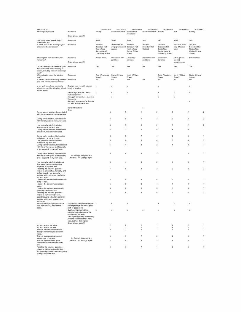
RespondentIDWhat is your job title? Response
Other (please specify)
How many hours a week do you spend at MCSI?
Response
In which area of the building is your primary work area located?
Response
Which option best describes your work area?
Response
Other (please specify)
Do you have outside views from your work area while either standing or seated, including windows above eye level?
Response
Which direction does the window face?
Response
Is there a corridor or hallway between your seat and the nearest window?
Response
In my work area, I can personally adjust or control the following. (Check all that apply):
Daylight level i.e., with window blinds or shades
Electric light level, i.e., with a switch or dimmerAir supply temperature i.e., with a thermostatAir supply volume and/or direction i.e., with an adjustable vent
None of the aboveOther
During warmer weather, I am satisfied with the temperature in my work area.
During cooler weather, I am satisfied with the temperature in my work area.
I am generally satisfied with the temperature in my work area.During warmer weather, I believe the air is too humid in my work area.
During cooler weather, I believe the air is too dry in my work area.I am generally satisfied with the humidity in my work area.During warmer weather, I am satisfied with the air flow speed (not too drafty or too stagnant) in my work area.
During cooler weather, I am satisfied with the air flow speed (not too drafty or too stagnant) in my work area.
I am generally satisfied with the air flow speed (not too drafty or too stagnant) in my work area.Recalling the previous questions related to temperature, humidity, and air flow speed, I am generally satisfied with the thermal comfort in my work area.I believe the air in my work area is not stuffy or stale.I believe the air in my work area is clean.I believe the air in my work area is generally free from odors.Recalling the previous questions related to stuffiness/staleness, cleanliness and odor, I am generally satisfied with the air quality in my work area.What type of lighting is provided at your work area? (Check all that apply.)
Daylighting (sunlight entering the building through windows, glass roof, or glass doors)Overhead lighting (lighting provided by the fixtures on the ceiling or on the walls)Task lighting (lighting provided by personal fixtures at one's work area, such as desk lights)Other (please specify)
My work area is too bright.My work area is too dark.There is an adequate amount of daylight in my area (leave blank if none).There is an adequate amount of electric light in my area.There is a problem with glare, reflections or contrast in my work area.Recalling the previous questions related to lighting and daylighting, I am generally satisfied with the lighting quality in my work area.
1 = Strongly disagree; 4 = Neutral; 7 = Strongly agree
1 = Strongly disagree; 4 = Neutral; 7 = Strongly agree
2453034559 2452104034 2452005526 2451968040 2451873253 2449203632 2435366623Faculty Graduate student Postdoctoral
researcherGraduate student Faculty Staff Faculty
30-40 30-40 30-40 >40 >40 30-40 >40
2nd floor Benedum Hall - East offices (facing plaza & Thackeray Street)
3rd floor MCSI wing (grad student space)
2nd floor Benedum Hall - North offices (facing O'Hara Street)
2nd floor Benedum Hall - Wet Lab
2nd floor Benedum Hall - East offices (facing plaza & Thackeray Street)
First floor MCSI wing (Mascaro suite)
2nd floor Benedum Hall - North offices (facing O'Hara Street)
Private office Open office with partitions
Laboratory benches
Open office with partitions
Laboratory benches
Other (please specify)
Private office
reception area
Yes Yes Yes No Yes Yes Yes
East (Thackeray Street)
North (O’Hara Street)
North (O’Hara Street)
East (Thackeray Street)
North (O’Hara Street)
North (O’Hara Street)
No No Yes No No No No
x x x x x
x x x x x x
x x x
x
x
5 5 1 2 2 2 2
5 5 5 2 2 2 2
5 5 5 2 3 2 2
2 3 5 4 4 4 1
3 3 7 4 2 4 1
5 6 3 4 3 4 7
5 4 3 2 4 3 7
5 4 3 2 3 7
5 4 3 2 4 3 7
5 6 3 2 2 2 3
6 5 3 4 2 5 7
6 6 2 4 1 4 7
5 6 3 5 1 4 7
5 6 3 5 1 5 7
x x x x x x
x x x x x x x
2 2 1 1 4 2 11 1 1 7 4 2 16 7 7 3 7 7
6 7 7 2 2 6 7
2 5 4 2 6 4 1
6 7 7 1 3 5 7
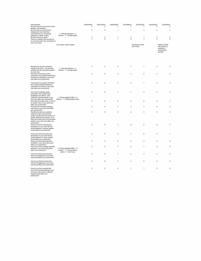
RespondentIDMy work area is too loud due to other people’s conversations.My work area is too loud due to background noise other than conversations (e.g. mechanical equipment, outdoor noises).My work area is too quiet.There is a problem with acoustics in my work area other than generally too loud or too quiet.
If you agree, please explain:
Recalling the previous questions related to acoustics, I am generally satisfied with the acoustical quality in my work area.
1 = Strongly disagree; 4 = Neutral; 7 = Strongly agree
How does the thermal comfort (remember, this includes temperature, humidity and airspeed) in your work area affect your productivity?
How does the air quality (remember, this includes stuffiness/staleness, cleanliness and odors) in your work area affect your productivity?
How does the lighting quality (remember, this includes both daylighting and artifical - both overhead, and task-based) in your work area affect your productivity?How does the outdoor view, or lack of an outdoor view, in your work area affect your productivity?How does the acoustical quality or noise level in your work area affect your productivity?Recalling the previous questions related to indoor environmental quality (including thermal comfort, air quality, lighting and acoustics), how does the overall indoor environmental quality in your work area affect your productivity?How do you think increasing the temperature in your work area by several degrees in warmer weather would affect your productivity?
How do you think decreasing the temperature in your work area by several degrees in cooler weather would affect your productivity?How do you think decreasing the ventilation in your work area would affect your productivity? How do you think including operable windows in your work area would affect your productivity?
How do you think decreasing the amount of daylighting in your work area would affect your productivity?
How do you think increasing the amount of daylighting in your work area would affect your productivity?
How do you think automatically turning off overhead lighting in your work area when there is sufficient daylight would affect your productivity?
1 = Strong negative effect; 4 = Neutral; 7 = Strong positive effect
1 = Strong negative effect; 4 = Neutral; 7 = Strong positive
effect; 0 = I don't know
1 = Strongly disagree; 4 = Neutral; 7 = Strongly agree
2453034559 2452104034 2452005526 2451968040 2451873253 2449203632 24353666236 3 1 3 7 6 5
5 6 1 7 7 4 1
3 4 7 2 1 2 21 2 1 6 7 2 5
mechanical noises from HVAC
Hallway outside office seems to resemble a reverberation chamber
4 4 6 1 1 4 3
4 5 2 4 3 4 3
4 5 2 4 1 4 4
3 6 7 2 3 5 5
4 6 2 4 6 5 7
4 4 7 3 1 4 3
4 6 3 4 3 4 4
2 5 7 6 4 5 7
3 5 6 1 4 5 1
4 3 4 5 3 0 4
4 0 7 4 7 4 4
4 2 1 4 3 2 2
4 5 7 4 5 4 4
4 5 4 1 1 5 4

RespondentIDWhat is your job title? Response
Other (please specify)
How many hours a week do you spend at MCSI?
Response
In which area of the building is your primary work area located?
Response
Which option best describes your work area?
Response
Other (please specify)
Do you have outside views from your work area while either standing or seated, including windows above eye level?
Response
Which direction does the window face?
Response
Is there a corridor or hallway between your seat and the nearest window?
Response
In my work area, I can personally adjust or control the following. (Check all that apply):
Daylight level i.e., with window blinds or shades
Electric light level, i.e., with a switch or dimmerAir supply temperature i.e., with a thermostatAir supply volume and/or direction i.e., with an adjustable vent
None of the aboveOther
During warmer weather, I am satisfied with the temperature in my work area.
During cooler weather, I am satisfied with the temperature in my work area.
I am generally satisfied with the temperature in my work area.During warmer weather, I believe the air is too humid in my work area.
During cooler weather, I believe the air is too dry in my work area.I am generally satisfied with the humidity in my work area.During warmer weather, I am satisfied with the air flow speed (not too drafty or too stagnant) in my work area.
During cooler weather, I am satisfied with the air flow speed (not too drafty or too stagnant) in my work area.
I am generally satisfied with the air flow speed (not too drafty or too stagnant) in my work area.Recalling the previous questions related to temperature, humidity, and air flow speed, I am generally satisfied with the thermal comfort in my work area.I believe the air in my work area is not stuffy or stale.I believe the air in my work area is clean.I believe the air in my work area is generally free from odors.Recalling the previous questions related to stuffiness/staleness, cleanliness and odor, I am generally satisfied with the air quality in my work area.What type of lighting is provided at your work area? (Check all that apply.)
Daylighting (sunlight entering the building through windows, glass roof, or glass doors)Overhead lighting (lighting provided by the fixtures on the ceiling or on the walls)Task lighting (lighting provided by personal fixtures at one's work area, such as desk lights)Other (please specify)
My work area is too bright.My work area is too dark.There is an adequate amount of daylight in my area (leave blank if none).There is an adequate amount of electric light in my area.There is a problem with glare, reflections or contrast in my work area.Recalling the previous questions related to lighting and daylighting, I am generally satisfied with the lighting quality in my work area.
1 = Strongly disagree; 4 = Neutral; 7 = Strongly agree
1 = Strongly disagree; 4 = Neutral; 7 = Strongly agree
2434857673 2434505183 2433360907 2431206899 2427574863 2427444506 2427321634Graduate student Graduate student Graduate student Faculty Faculty Graduate student Faculty
10-20 10-20 >40 >40 >40 20-30 >40
2nd floor MCSI wing (grad student space or dry lab)
2nd floor MCSI wing (grad student space or dry lab)
3rd floor MCSI wing (grad student space)
2nd floor MCSI wing (grad student space or dry lab)
2nd floor Benedum Hall - North offices (facing O'Hara Street)
2nd floor MCSI wing (grad student space or dry lab)
2nd floor Benedum Hall - North offices (facing O'Hara Street)
Open office with partitions
Open office with partitions
Open office with partitions
Private office Private office Open office with partitions
Private office
No Yes Yes Yes Yes Yes Yes
North (O’Hara Street)
North (O’Hara Street)
North (O’Hara Street)
East (Thackeray Street)
North (O’Hara Street)
North (O’Hara Street)
North (O’Hara Street)
No No No No No No No
x x x x x x
x x x x
x
x
5 4 4 4 1 6 4
4 4 6 4 5 6 4
4 4 5 4 3 6 5
2 3 4 5 6 2 3
2 3 4 5 6 2 5
6 5 4 5 6 6 5
6 4 5 5 6 6 5
6 4 5 5 5 6 5
6 5 5 5 5 6 5
7 5 5 4 2 6 5
6 5 6 5 5 6 6
6 5 6 5 5 5 6
4 5 6 5 2 6 5
6 5 6 5 2 6 5
x x x x x x
x x x x x x x
x x
2 3 2 3 4 2 12 3 3 6 4 2 12 5 6 5 6 5 7
4 5 6 6 6 7 7
2 4 5 4 3 2 1
6 5 6 4 5 6 7

RespondentIDMy work area is too loud due to other people’s conversations.My work area is too loud due to background noise other than conversations (e.g. mechanical equipment, outdoor noises).My work area is too quiet.There is a problem with acoustics in my work area other than generally too loud or too quiet.
If you agree, please explain:
Recalling the previous questions related to acoustics, I am generally satisfied with the acoustical quality in my work area.
1 = Strongly disagree; 4 = Neutral; 7 = Strongly agree
How does the thermal comfort (remember, this includes temperature, humidity and airspeed) in your work area affect your productivity?
How does the air quality (remember, this includes stuffiness/staleness, cleanliness and odors) in your work area affect your productivity?
How does the lighting quality (remember, this includes both daylighting and artifical - both overhead, and task-based) in your work area affect your productivity?How does the outdoor view, or lack of an outdoor view, in your work area affect your productivity?How does the acoustical quality or noise level in your work area affect your productivity?Recalling the previous questions related to indoor environmental quality (including thermal comfort, air quality, lighting and acoustics), how does the overall indoor environmental quality in your work area affect your productivity?How do you think increasing the temperature in your work area by several degrees in warmer weather would affect your productivity?
How do you think decreasing the temperature in your work area by several degrees in cooler weather would affect your productivity?How do you think decreasing the ventilation in your work area would affect your productivity? How do you think including operable windows in your work area would affect your productivity?
How do you think decreasing the amount of daylighting in your work area would affect your productivity?
How do you think increasing the amount of daylighting in your work area would affect your productivity?
How do you think automatically turning off overhead lighting in your work area when there is sufficient daylight would affect your productivity?
1 = Strong negative effect; 4 = Neutral; 7 = Strong positive effect
1 = Strong negative effect; 4 = Neutral; 7 = Strong positive
effect; 0 = I don't know
1 = Strongly disagree; 4 = Neutral; 7 = Strongly agree
2434857673 2434505183 2433360907 2431206899 2427574863 2427444506 24273216345 4 4 7 3 2 1
5 3 4 7 3 2 1
2 3 1 1 4 3 12 3 1 7 4 2 1
Echos, conversations, etc. -- sometimes its hard to concentrate
4 5 5 1 6 6 7
5 4 4 4 3 5 3
5 4 4 5 3 4 3
7 4 6 6 6 6 4
7 4 6 7 7 4 4
7 4 5 7 6 4 4
7 4 5 6 3 4 4
0 5 3 4 7 3 4
0 2 3 4 2 4 3
3 3 0 4 4 3 3
6 5 6 4 4 5 7
3 1 2 6 3 1
6 7 6 6 4 5 4
7 5 4 5 4 5 4
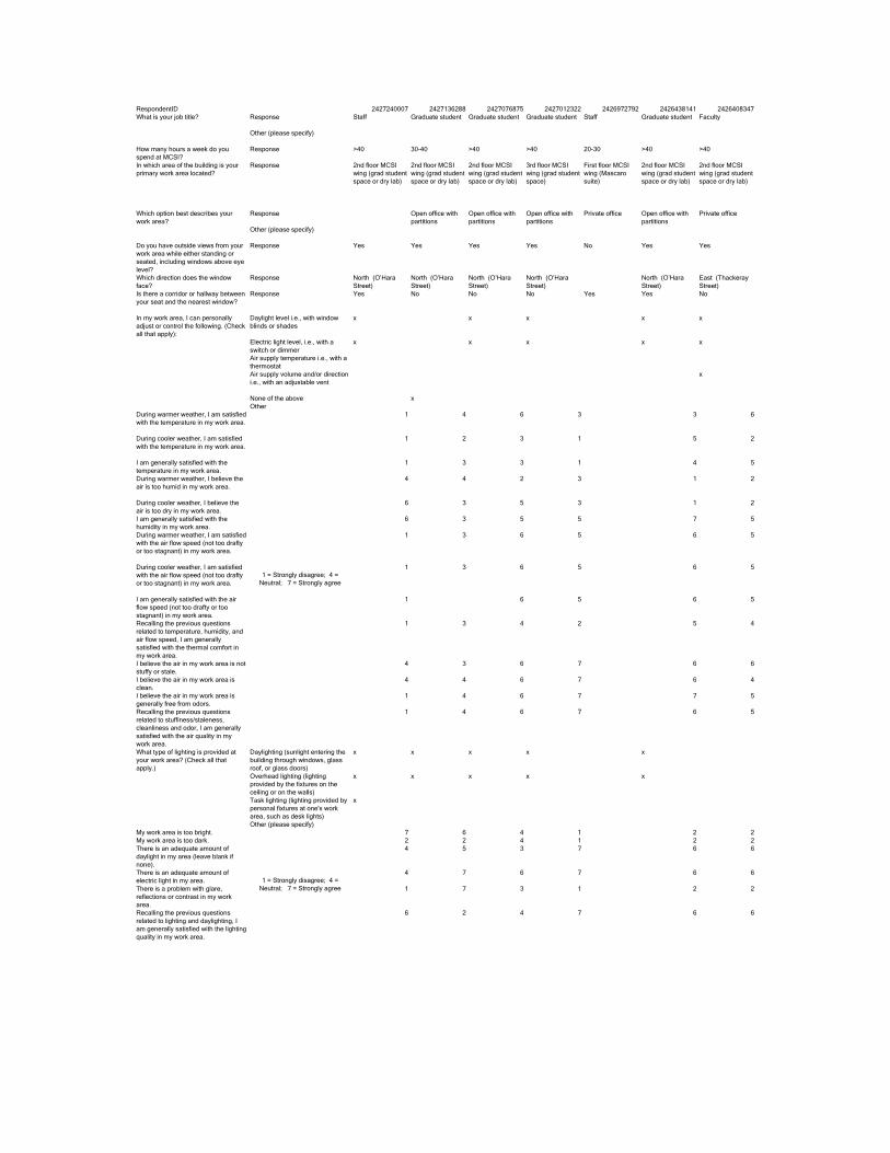
RespondentIDWhat is your job title? Response
Other (please specify)
How many hours a week do you spend at MCSI?
Response
In which area of the building is your primary work area located?
Response
Which option best describes your work area?
Response
Other (please specify)
Do you have outside views from your work area while either standing or seated, including windows above eye level?
Response
Which direction does the window face?
Response
Is there a corridor or hallway between your seat and the nearest window?
Response
In my work area, I can personally adjust or control the following. (Check all that apply):
Daylight level i.e., with window blinds or shades
Electric light level, i.e., with a switch or dimmerAir supply temperature i.e., with a thermostatAir supply volume and/or direction i.e., with an adjustable vent
None of the aboveOther
During warmer weather, I am satisfied with the temperature in my work area.
During cooler weather, I am satisfied with the temperature in my work area.
I am generally satisfied with the temperature in my work area.During warmer weather, I believe the air is too humid in my work area.
During cooler weather, I believe the air is too dry in my work area.I am generally satisfied with the humidity in my work area.During warmer weather, I am satisfied with the air flow speed (not too drafty or too stagnant) in my work area.
During cooler weather, I am satisfied with the air flow speed (not too drafty or too stagnant) in my work area.
I am generally satisfied with the air flow speed (not too drafty or too stagnant) in my work area.Recalling the previous questions related to temperature, humidity, and air flow speed, I am generally satisfied with the thermal comfort in my work area.I believe the air in my work area is not stuffy or stale.I believe the air in my work area is clean.I believe the air in my work area is generally free from odors.Recalling the previous questions related to stuffiness/staleness, cleanliness and odor, I am generally satisfied with the air quality in my work area.What type of lighting is provided at your work area? (Check all that apply.)
Daylighting (sunlight entering the building through windows, glass roof, or glass doors)Overhead lighting (lighting provided by the fixtures on the ceiling or on the walls)Task lighting (lighting provided by personal fixtures at one's work area, such as desk lights)Other (please specify)
My work area is too bright.My work area is too dark.There is an adequate amount of daylight in my area (leave blank if none).There is an adequate amount of electric light in my area.There is a problem with glare, reflections or contrast in my work area.Recalling the previous questions related to lighting and daylighting, I am generally satisfied with the lighting quality in my work area.
1 = Strongly disagree; 4 = Neutral; 7 = Strongly agree
1 = Strongly disagree; 4 = Neutral; 7 = Strongly agree
2427240007 2427136288 2427076875 2427012322 2426972792 2426438141 2426408347Staff Graduate student Graduate student Graduate student Staff Graduate student Faculty
>40 30-40 >40 >40 20-30 >40 >40
2nd floor MCSI wing (grad student space or dry lab)
2nd floor MCSI wing (grad student space or dry lab)
2nd floor MCSI wing (grad student space or dry lab)
3rd floor MCSI wing (grad student space)
First floor MCSI wing (Mascaro suite)
2nd floor MCSI wing (grad student space or dry lab)
2nd floor MCSI wing (grad student space or dry lab)
Open office with partitions
Open office with partitions
Open office with partitions
Private office Open office with partitions
Private office
Yes Yes Yes Yes No Yes Yes
North (O’Hara Street)
North (O’Hara Street)
North (O’Hara Street)
North (O’Hara Street)
North (O’Hara Street)
East (Thackeray Street)
Yes No No No Yes Yes No
x x x x x
x x x x x
x
x
1 4 6 3 3 6
1 2 3 1 5 2
1 3 3 1 4 5
4 4 2 3 1 2
6 3 5 3 1 2
6 3 5 5 7 5
1 3 6 5 6 5
1 3 6 5 6 5
1 6 5 6 5
1 3 4 2 5 4
4 3 6 7 6 6
4 4 6 7 6 4
1 4 6 7 7 5
1 4 6 7 6 5
x x x x x
x x x x x
x
7 6 4 1 2 22 2 4 1 2 24 5 3 7 6 6
4 7 6 7 6 6
1 7 3 1 2 2
6 2 4 7 6 6

RespondentIDMy work area is too loud due to other people’s conversations.My work area is too loud due to background noise other than conversations (e.g. mechanical equipment, outdoor noises).My work area is too quiet.There is a problem with acoustics in my work area other than generally too loud or too quiet.
If you agree, please explain:
Recalling the previous questions related to acoustics, I am generally satisfied with the acoustical quality in my work area.
1 = Strongly disagree; 4 = Neutral; 7 = Strongly agree
How does the thermal comfort (remember, this includes temperature, humidity and airspeed) in your work area affect your productivity?
How does the air quality (remember, this includes stuffiness/staleness, cleanliness and odors) in your work area affect your productivity?
How does the lighting quality (remember, this includes both daylighting and artifical - both overhead, and task-based) in your work area affect your productivity?How does the outdoor view, or lack of an outdoor view, in your work area affect your productivity?How does the acoustical quality or noise level in your work area affect your productivity?Recalling the previous questions related to indoor environmental quality (including thermal comfort, air quality, lighting and acoustics), how does the overall indoor environmental quality in your work area affect your productivity?How do you think increasing the temperature in your work area by several degrees in warmer weather would affect your productivity?
How do you think decreasing the temperature in your work area by several degrees in cooler weather would affect your productivity?How do you think decreasing the ventilation in your work area would affect your productivity? How do you think including operable windows in your work area would affect your productivity?
How do you think decreasing the amount of daylighting in your work area would affect your productivity?
How do you think increasing the amount of daylighting in your work area would affect your productivity?
How do you think automatically turning off overhead lighting in your work area when there is sufficient daylight would affect your productivity?
1 = Strong negative effect; 4 = Neutral; 7 = Strong positive effect
1 = Strong negative effect; 4 = Neutral; 7 = Strong positive
effect; 0 = I don't know
1 = Strongly disagree; 4 = Neutral; 7 = Strongly agree
2427240007 2427136288 2427076875 2427012322 2426972792 2426438141 24264083475 4 3 4 5 2
7 4 2 1 5 2
1 4 3 1 2 26 4 2 1 2 2
constant noise from air duct that supply the whole floor MCSI and Benedum; poor workmanship (sound insulation) of the duct itself plus gaps and unsealed duct joints
1 4 5 6 5 6
1 6 4 3 6 3
2 6 5 6 6 4
5 7 4 6 7 4
4 7 3 6 7 5
1 4 5 4 3 4
1 6 5 5 6 4
3 7 5 7 7 2
5 7 1 1 2 2
0 6 3 3 0 3
4 4 5 4 7 4
0 7 1 1 1 4
0 7 7 6 7 4
4 5 6 4 2 4

RespondentIDWhat is your job title? Response
Other (please specify)
How many hours a week do you spend at MCSI?
Response
In which area of the building is your primary work area located?
Response
Which option best describes your work area?
Response
Other (please specify)
Do you have outside views from your work area while either standing or seated, including windows above eye level?
Response
Which direction does the window face?
Response
Is there a corridor or hallway between your seat and the nearest window?
Response
In my work area, I can personally adjust or control the following. (Check all that apply):
Daylight level i.e., with window blinds or shades
Electric light level, i.e., with a switch or dimmerAir supply temperature i.e., with a thermostatAir supply volume and/or direction i.e., with an adjustable vent
None of the aboveOther
During warmer weather, I am satisfied with the temperature in my work area.
During cooler weather, I am satisfied with the temperature in my work area.
I am generally satisfied with the temperature in my work area.During warmer weather, I believe the air is too humid in my work area.
During cooler weather, I believe the air is too dry in my work area.I am generally satisfied with the humidity in my work area.During warmer weather, I am satisfied with the air flow speed (not too drafty or too stagnant) in my work area.
During cooler weather, I am satisfied with the air flow speed (not too drafty or too stagnant) in my work area.
I am generally satisfied with the air flow speed (not too drafty or too stagnant) in my work area.Recalling the previous questions related to temperature, humidity, and air flow speed, I am generally satisfied with the thermal comfort in my work area.I believe the air in my work area is not stuffy or stale.I believe the air in my work area is clean.I believe the air in my work area is generally free from odors.Recalling the previous questions related to stuffiness/staleness, cleanliness and odor, I am generally satisfied with the air quality in my work area.What type of lighting is provided at your work area? (Check all that apply.)
Daylighting (sunlight entering the building through windows, glass roof, or glass doors)Overhead lighting (lighting provided by the fixtures on the ceiling or on the walls)Task lighting (lighting provided by personal fixtures at one's work area, such as desk lights)Other (please specify)
My work area is too bright.My work area is too dark.There is an adequate amount of daylight in my area (leave blank if none).There is an adequate amount of electric light in my area.There is a problem with glare, reflections or contrast in my work area.Recalling the previous questions related to lighting and daylighting, I am generally satisfied with the lighting quality in my work area.
1 = Strongly disagree; 4 = Neutral; 7 = Strongly agree
1 = Strongly disagree; 4 = Neutral; 7 = Strongly agree
2425689242 2425258234 2425246112 2425204363 2425191480 2425175758 2425022099Undergraduate student
Graduate student Graduate student Graduate student Graduate student Graduate student
research associate
10-20 >40 30-40 30-40 20-30 30-40 30-40
3rd floor MCSI wing (grad student space)
3rd floor MCSI wing (grad student space)
3rd floor MCSI wing (grad student space)
3rd floor MCSI wing (grad student space)
3rd floor MCSI wing (grad student space)
3rd floor MCSI wing (grad student space)
2nd floor Benedum Hall - Wet Lab
Open office with partitions
Open office with partitions
Open office with partitions
Open office with partitions
Open office with partitions
Open office with partitions
Other (please specify)Open laboratory space
Yes Yes Yes Yes No Yes No
North (O’Hara Street)
North (O’Hara Street)
North (O’Hara Street)
North (O’Hara Street)
North (O’Hara Street)
No Yes No No No No No
x x x x x
x x x x
2 6 5 3 5 4 1
2 5 6 3 5 3 5
2 6 6 4 5 3 3
3 3 1 3 2 2 4
3 6 2 3 2 2 2
5 3 6 3 6 6 4
5 5 6 5 4 3 5
5 5 6 6 4 3 5
5 5 6 6 4 3 5
3 6 7 4 5 3 3
6 6 7 5 5 6 6
6 6 7 6 5 6 5
6 6 7 5 5 6 5
6 6 7 5 5 6 5
x x x x x x
x x x x x x x
x x
2 5 3 2 1 2 33 3 3 2 4 2 55 6 7 6 2 6 5
5 5 7 6 6 6 5
1 7 3 3 5 6 1
5 5 7 6 3 6 4

RespondentIDMy work area is too loud due to other people’s conversations.My work area is too loud due to background noise other than conversations (e.g. mechanical equipment, outdoor noises).My work area is too quiet.There is a problem with acoustics in my work area other than generally too loud or too quiet.
If you agree, please explain:
Recalling the previous questions related to acoustics, I am generally satisfied with the acoustical quality in my work area.
1 = Strongly disagree; 4 = Neutral; 7 = Strongly agree
How does the thermal comfort (remember, this includes temperature, humidity and airspeed) in your work area affect your productivity?
How does the air quality (remember, this includes stuffiness/staleness, cleanliness and odors) in your work area affect your productivity?
How does the lighting quality (remember, this includes both daylighting and artifical - both overhead, and task-based) in your work area affect your productivity?How does the outdoor view, or lack of an outdoor view, in your work area affect your productivity?How does the acoustical quality or noise level in your work area affect your productivity?Recalling the previous questions related to indoor environmental quality (including thermal comfort, air quality, lighting and acoustics), how does the overall indoor environmental quality in your work area affect your productivity?How do you think increasing the temperature in your work area by several degrees in warmer weather would affect your productivity?
How do you think decreasing the temperature in your work area by several degrees in cooler weather would affect your productivity?How do you think decreasing the ventilation in your work area would affect your productivity? How do you think including operable windows in your work area would affect your productivity?
How do you think decreasing the amount of daylighting in your work area would affect your productivity?
How do you think increasing the amount of daylighting in your work area would affect your productivity?
How do you think automatically turning off overhead lighting in your work area when there is sufficient daylight would affect your productivity?
1 = Strong negative effect; 4 = Neutral; 7 = Strong positive effect
1 = Strong negative effect; 4 = Neutral; 7 = Strong positive
effect; 0 = I don't know
1 = Strongly disagree; 4 = Neutral; 7 = Strongly agree
2425689242 2425258234 2425246112 2425204363 2425191480 2425175758 24250220993 7 3 3 2 3 3
3 5 4 6 2 6 3
3 2 1 6 5 2 23 4 1 2 2 2 3
6 4 6 5 5 2 5
3 5 4 3 3 3 2
5 6 4 5 5 6 4
5 6 6 7 2 6 4
5 4 6 7 2 5 5
4 4 4 3 4 5 5
4 5 5 5 3 4 4
6 3 4 6 3 4 1
1 5 4 2 1 2 1
4 4 5 3 4 5 1
4 4 5 4 6 1
3 3 2 3 2 2 1
4 3 3 4 7 5 5
3 4 4 4 0 4 4

RespondentIDWhat is your job title? Response
Other (please specify)
How many hours a week do you spend at MCSI?
Response
In which area of the building is your primary work area located?
Response
Which option best describes your work area?
Response
Other (please specify)
Do you have outside views from your work area while either standing or seated, including windows above eye level?
Response
Which direction does the window face?
Response
Is there a corridor or hallway between your seat and the nearest window?
Response
In my work area, I can personally adjust or control the following. (Check all that apply):
Daylight level i.e., with window blinds or shades
Electric light level, i.e., with a switch or dimmerAir supply temperature i.e., with a thermostatAir supply volume and/or direction i.e., with an adjustable vent
None of the aboveOther
During warmer weather, I am satisfied with the temperature in my work area.
During cooler weather, I am satisfied with the temperature in my work area.
I am generally satisfied with the temperature in my work area.During warmer weather, I believe the air is too humid in my work area.
During cooler weather, I believe the air is too dry in my work area.I am generally satisfied with the humidity in my work area.During warmer weather, I am satisfied with the air flow speed (not too drafty or too stagnant) in my work area.
During cooler weather, I am satisfied with the air flow speed (not too drafty or too stagnant) in my work area.
I am generally satisfied with the air flow speed (not too drafty or too stagnant) in my work area.Recalling the previous questions related to temperature, humidity, and air flow speed, I am generally satisfied with the thermal comfort in my work area.I believe the air in my work area is not stuffy or stale.I believe the air in my work area is clean.I believe the air in my work area is generally free from odors.Recalling the previous questions related to stuffiness/staleness, cleanliness and odor, I am generally satisfied with the air quality in my work area.What type of lighting is provided at your work area? (Check all that apply.)
Daylighting (sunlight entering the building through windows, glass roof, or glass doors)Overhead lighting (lighting provided by the fixtures on the ceiling or on the walls)Task lighting (lighting provided by personal fixtures at one's work area, such as desk lights)Other (please specify)
My work area is too bright.My work area is too dark.There is an adequate amount of daylight in my area (leave blank if none).There is an adequate amount of electric light in my area.There is a problem with glare, reflections or contrast in my work area.Recalling the previous questions related to lighting and daylighting, I am generally satisfied with the lighting quality in my work area.
1 = Strongly disagree; 4 = Neutral; 7 = Strongly agree
1 = Strongly disagree; 4 = Neutral; 7 = Strongly agree
2424969194 2424967816 2424902461 2424885322 2424821753 2424790460 2424784869Graduate student Postdoctoral
researcherGraduate student Faculty Graduate student Faculty Faculty
30-40 >40 20-30 >40 20-30 >40 >40
2nd floor Benedum Hall - Wet Lab
3rd floor MCSI wing (grad student space)
3rd floor MCSI wing (grad student space)
3rd floor MCSI wing (grad student space)
2nd floor MCSI wing (grad student space or dry lab)
2nd floor Benedum Hall - East offices (facing plaza & Thackeray Street)
First floor MCSI wing (Mascaro suite)
Open office with partitions
Open office with partitions
Open office with partitions
Open office with partitions
Open office with partitions
Private office Private office
Yes Yes Yes Yes Yes Yes Yes
South (Fifth Avenue)
North (O’Hara Street)
North (O’Hara Street)
East (Thackeray Street)
North (O’Hara Street)
East (Thackeray Street)
North (O’Hara Street)
No No No Yes No No No
x x x x x
x x x x
x x x
x
4 5 7 2 3 3 6
4 5 7 4 2 1 5
4 5 7 3 2 2 6
2 3 7 4 1 4 2
3 5 7 4 5 4 6
4 4 4 6 4 4
4 5 7 2 7 4 6
4 5 7 2 6 4 6
4 5 7 2 6 4 6
4 5 7 3 3 2 6
4 6 7 4 7 4 6
4 6 7 4 7 3 6
6 6 7 4 7 3 6
5 6 7 4 7 4 6
x x x x
x x x x x x x
x x
4 2 1 4 1 4 24 2 1 4 1 2 24 7 7 4 5 2 6
5 6 7 4 7 6 6
3 5 5 4 4 1 2
5 6 7 4 5 4 6

RespondentIDMy work area is too loud due to other people’s conversations.My work area is too loud due to background noise other than conversations (e.g. mechanical equipment, outdoor noises).My work area is too quiet.There is a problem with acoustics in my work area other than generally too loud or too quiet.
If you agree, please explain:
Recalling the previous questions related to acoustics, I am generally satisfied with the acoustical quality in my work area.
1 = Strongly disagree; 4 = Neutral; 7 = Strongly agree
How does the thermal comfort (remember, this includes temperature, humidity and airspeed) in your work area affect your productivity?
How does the air quality (remember, this includes stuffiness/staleness, cleanliness and odors) in your work area affect your productivity?
How does the lighting quality (remember, this includes both daylighting and artifical - both overhead, and task-based) in your work area affect your productivity?How does the outdoor view, or lack of an outdoor view, in your work area affect your productivity?How does the acoustical quality or noise level in your work area affect your productivity?Recalling the previous questions related to indoor environmental quality (including thermal comfort, air quality, lighting and acoustics), how does the overall indoor environmental quality in your work area affect your productivity?How do you think increasing the temperature in your work area by several degrees in warmer weather would affect your productivity?
How do you think decreasing the temperature in your work area by several degrees in cooler weather would affect your productivity?How do you think decreasing the ventilation in your work area would affect your productivity? How do you think including operable windows in your work area would affect your productivity?
How do you think decreasing the amount of daylighting in your work area would affect your productivity?
How do you think increasing the amount of daylighting in your work area would affect your productivity?
How do you think automatically turning off overhead lighting in your work area when there is sufficient daylight would affect your productivity?
1 = Strong negative effect; 4 = Neutral; 7 = Strong positive effect
1 = Strong negative effect; 4 = Neutral; 7 = Strong positive
effect; 0 = I don't know
1 = Strongly disagree; 4 = Neutral; 7 = Strongly agree
2424969194 2424967816 2424902461 2424885322 2424821753 2424790460 24247848696 5 5 4 2 7 5
6 5 1 7 6 5 5
1 1 1 1 1 1 24 1 2 4 1 7 2
too many hard reflective surfaces - entire area echoes
1 3 6 1 3 1 4
4 4 6 4 3 4 4
4 5 6 4 4 4 4
4 5 7 4 4 4 5
2 7 6 4 2 2 5
1 4 2 1 3 2 3
3 5 6 2 3 3 4
5 4 4 7 6 5 2
2 4 1 1 2 1 4
4 4 0 2 0 3 3
6 6 5 4 6 5 7
4 2 1 2 2 1 3
4 6 4 5 5 5 6
4 6 4 1 4 0 4

Question Number of responses
You should ask what the occupants of the building think of those who designed the building. My opinion of them is strongly negative. The building might be friendly to environment but it is unfriendly, almost hostile to the occupants.
Dimming light switches or automated dimming. Lower air flow rate (?) for less noisy air flow. Warmer temperatures in warm months, usually I am to cold in the office during warm months. During cold months, I am not too warm. I am sometimes still cold, but can add clothing and drink hot beverages. Also, modifying workspace orientation to use daylighting but reduce glare my be helpful.Noise reduction, better thermal control.N/AIt is typically too cold most of the year, though it has been slightly better lately. There is constant white noise from possibly air vents that can be bothersome at times. It may be nice if we were allowed to dim the lights.The cubicles on the right side of the 3rd floor grad space often need electric lighting even though there is enough day lighting present. Theres a wide mismatch between day lighting present in cubicles by the window and those not by the windowThe timer on the motion sensor lighting is wayyy too short. It's very annoying to have to get up everyday when I'm working at my desk and put the lights back on.Auto light shut off in corridors and esp bathrooms is dangerous. In offices it is annoying to wave my arms around every 5 minutes. Sound is horrendous. Smells from Basement food court (burnt bagels) every morning makes me nauseous.Probably make it more scenic. As in put some plants around the building. Looking at concrete doesn't increase productivity for sure.The sensors on the automatic bathroom fixtures seem to be using more water than previous hand fixtures (ie. the toilet flushes multiple times for a single person's use)1. I would prefer to have a control over over my temperature directly in my office. (It is typically very cold in the summer.) 2. The odor of the cooking food from the kitchen downstairs is often way too strong and offensive (especially in the mornings). I often get severe headaches from the strong odors --It does impact my productivity.The kitchen on the basement that dumps strong odour and smoke of burning food. There is no ventilation on the kitchen area, so the second floor smell really bad for hours per day. Temperature difference between office (appr 70F), corridor (appr 60F) and bathroom (sometime 80F) do not create healthy environment. My place do not have temperature control, so I'm at mercy other's lab dwellers.
I wish I could open the windows.
label the switches for the ceiling lights.It often feels too cold in the summer, when people are dressed for warmer weather anyway.
More individual thermostat, lighting and, if possible, window control. Less fan noise and drafts.Turn the temperature up during cooler months. The lighting timing is fine (automatics) - although the lights themselves burn out a lot. I'm not sure if that is the type of light or the contractor used.Too noisy
Response text
Ventilation seems to be fine. I don't mind the room being a bit warmer and "normal" in the summer and a bit "cooler" than normal in the winter, but the problem I have is that the floor heating next to the window doesn't seem to be adequate, so in (very) cold weather the ventilation heating does not compensate for the heat loss through the windows, and the room is cold. Otherwise I'm happy with the conditions and control that i have in the room (the adjustable vent is nice to have).
Do you have any other suggestions for improving the MCSI building? If so, what are they?
It didn't take 30 minutes, that was somewhat misleading to me, so the updated communication was helpful and encouraged me to participate knowing 15-20minutes was a more manageable expectation.
8
23
Do you have any suggestions for improving this survey? If so, what are they? N/A
Discuss cleanliness, elevator malfunctions, bathrooms, water fountains, staircases, open spaces.The MCSI building has a conference rooms at each floor that are not included in survey Would be interesting to see correlation between how green occupants are (their knowledge about green buildings or how important they think energy use is) and how they respond to certain questionssuggestions for common areas for leftover food, cutlery, etc; students in this area are very good about re-distributing, but collection of give-aways has become high with graduating students.
There were no questions regarding raising the temperature in the winter (ie. problem with building being too cold in winter).
better noise insulation between external classroom area and office spaceImprove operation of HVAC system. Check if the level of noise in the office areas are within the safety limits established by OSHA.Provide more non-sky outside views in 2nd floor dry lab workspaces. Reduce vent noise in same area ceiling, which sounds like an rain storm at times.
Too many to list - many aspects of the design have proven to be a dismal failure; not least of which is the net loss of space used to support the school missions when the intent of the renovation scheme was to increase space.
I think having better food preparation and storage areas would improve user eating habits.

168
BIBLIOGRAPHY
2030 (2011) Architecture 2030: About Us. Architecture2030.org. http://architecture2030.org/about/about_us. Accessed Feb 11 2013
Abdou OA (1997) Effects of luminous environment on worker productivity in building spaces. Journal of Architectural Engineering 3 (3)
ACHD (2011) Air Quality Annual Report for 2010 with 1990-2010 Trends. Allegheny County Health Department, Air Quality Program, Pittsburgh, PA
AirCuity OptiNet Overview~. http://www.aircuity.com/technology/optinet-overview/. Accessed September 24, 2012
Aktas CB, Bilec MM (2012) Impact of lifetime on US residential building LCA results. International Journal of Life Cycle Assessment 17 (3):337-349. doi:10.1007/s11367-011-0363-x
ANL (2010) GREET Model: The Greenhouse gases, Regulated Emissions, and Energy use in Transportation Model, version 1.8d.1.
ASHRAE (2009) 2009 ASHRAE Handbook (Fundamentals). American Society of Heating, Refrigeration and Air Conditioning Engineers (ASHRAE),
ASHRAE (2010) ANSI/ASHRAE Standard 62.1-2010, Ventilation for Acceptable Indoor Air Quality. American Society of Heating, Refrigeration and Air Conditioning Engineers (ASHRAE), Atlanta, GA
Atkinson RW, Fuller GW, Anderson HR, Harrison RM, Armstrong B (2010) Urban ambient particle metrics and health: A time-series analysis. Epidemiology 21 (4):501-511. doi:10.1097/EDE.0b013e3181debc88
Bare J (2011) TRACI 2.0: the tool for the reduction and assessment of chemical and other environmental impacts 2.0. Clean Technology and Environmental Policy. doi:10.1007/s10098-101-0338-9
Bare J, Norris GA, Pennington DW, McKone T (2003) TRACI: The Tool for the Reduction and Assessment of Chemical and Other Environmental Impacts. Journal of Industrial Ecology 6:49-78

169
Bennett DH, McKone TE, Evans JS, Nazaroff WW, Margni MD, Jolliet O, Smith KR (2002) Defining intake fraction. Environmental Science and Technology 36 (9):206A-211A
Bergin S, Shih J-S, Krupnick A, Boylan J, Wilkinson J, Odman M, Russell A (2007) Regional Air Quality: Local and Interstate Impacts of NOx and SO2 Emissions on Ozone and Fine Particulate Matter in the Eastern United States. Environmental Science & Techology 41:4677-4689
Bilec M, Ries R, Matthews HS, Sharrard, A.L. (2006) Example of a hybrid life-cycle assessment of construction processes. Journal of Infrastructure Systems 12 (4):207-215
Bilec MM, Ries RJ, Matthews HS (2010) Life-cycle assessment modeling of construction processes for buildings. Journal of Infrastructure Systems 16 (3):199-205. doi:10.1061/(asce)is.1943-555x.0000022
Choi JH, Loftness V, Aziz A (2012) Post-occupancy evaluation of 20 office buildings as basis for future IEQ standards and guidelines. Energy and Buildings 46:167-175. doi:10.1016/j.enbuild.2011.08.009
Collinge WO, Landis AE, Jones AK, Schaefer LA, Bilec MM (2012a) Dynamic life cycle assessment: framework and application to an institutional building. International Journal of Life Cycle Assessment:1-15. doi:10.1007/s11367-012-0528-2
Collinge WO, Landis AE, Jones AK, Schaefer LA, Bilec MM Integrating indoor environmental quality metrics in a dynamic life cycle assessment framework for buildings. In, Boston, MA, 2012b. 2012 IEEE International Symposium on Sustainable Systems and Technology, ISSST 2012.
Cucurachi S, Heijungs R, Ohlau K (2012) Towards a general framework for including noise impacts in LCA. International Journal of Life Cycle Assessment 17 (4):471-487. doi:10.1007/s11367-011-0377-4
Demou E, Hellweg S, Wilson MP, Hammond SK, McKone TE (2009) Evaluating indoor exposure modeling alternatives for LCA: A case study in the vehicle repair industry. Environmental Science and Technology 43 (15):5804-5810. doi:10.1021/es803551y
Dong BA, Lam KP, Hoynck M, Chiou YS, Zhang R, Benitez D (2010 (In Press)) An information technology enabled sustainability test-bed (ITEST) for occupancy detection through an environmental sensing network. Energy and Buildings
DRA (1965) Deeter and Richey Architects: Drawings for Construction of School of Engineering Building, University of Pittsburgh. General State Authority of the Commonwealth of Pennsylvania,
ecoinvent (2010) ecoinvent v2.2 database.
Edge (2007) Drawings for Construction of Benedum Hall: Upgrade and Deferred Maintenance for Buildings and Systems. University of Pittsburgh, Pittsburgh, PA

170
Edge (2008) Drawings for Construction of Benedum Hall: MSI Addition and Renovation. University of Pittsburgh, Pittsburgh, PA
Edwards L, Torcellini P (2002) A Literature Review of the Effects of Natural Light on Building Occupants. National Renewal Energy Laboratory (NREL), Golden, CO
Ekvall T, Weidema BP (2004) System boundaries and input data in consequential life cycle inventory analysis. International Journal of Life Cycle Assessment 9 (3):161-171
Emmerich SJ, Persily AK (1997) Literature review on CO2-based demand-controlled ventilation. ASHRAE Transactions 103 (pt 2):229-243
Fava JA, Denison R, Jones B, Curran MA, Vignon B, Selke S, Barnum J (1991) A Technical Framework for Life-Cycle Assessment. SETAC and SETAC Foundation for Environmental Education, Washington, DC
Field F, Kirchain R, Clark J (2000) Life-cycle assessment and temporal distributions of emissions: Developing a fleet-based analysis. Journal of Industrial Ecology 4 (2):71-91. doi:10.1162/108819800569816
Fisk WJ (2002) How IEQ affects health, productivity. ASHRAE Journal 44 (5):56+58-60
Fisk WJ, Black D, Brunner G (2011) Benefits and costs of improved IEQ in U.S. offices. Indoor Air 21 (5):357-367. doi:10.1111/j.1600-0668.2011.00719.x
Fisk WJ, Mirer AG, Mendell MJ (2009) Quantitative relationship of sick building syndrome symptoms with ventilation rates. Indoor Air 19 (2):159-165
Fisk WJ, Mirer AG, Mendell, M.J. (2009) Quantitative relationship of sick building syndrome symptoms with ventilation rates. Indoor Air 19:159-165
Frontczak M, Schiavon S, Goins J, Arens E, Zhang H, Wargocki P (2012) Quantitative relationships between occupant satisfaction and satisfaction aspects of indoor environmental quality and building design. Indoor Air 22 (2):119-131. doi:10.1111/j.1600-0668.2011.00745.x
Griffith B, Long, N., Torcellini, P., Judkoff, R., Crawley, D., and Ryan, J. (2007) Assessment of the Technical Potential for Achieving Net Zero-Energy Buildings in the Commercial Sector. National Renewable Energy Laboratory, Operated for the U.S. Department of Energy, Office of Energy Efficiency and Renewable Energy by Midwest Research Institute,
Heijungs R, Suh S (2002) The Computational Structure of Life Cycle Assessment. Kluwer Academic Publishers, Dordrecht, The Netherlands
Hellweg S, Demou E, Bruzzi R, Meijer A, Rosenbaum R, Huijbregts M, McKone T (2009) Integrating Human Indoor Air Pollutant Exposure within Life Cycle Impact Assessment. Environmental Science & Technology 43 (6)

171
Hellweg S, Frischknecht R (2004) Evaluation of long-term impacts in LCA. International Journal of Life Cycle Assessment 9 (5):339-340
Hellweg S, Hofstetter TB, Hungerbühler K (2003) Discounting and the environment: Should current impacts be weighted differently than impacts harming future generations? International Journal of Life Cycle Assessment 8 (1):8-18
Hellweg SD, E.; Bruzzi, R.; Meijer, A.; Rosenbaum, R.; Huijbregts, M.; McKone, T. (2009) Integrating human indoor air pollutant exposure within life cycle impact assessment. Environmental Science & Technology 43 (6):1670-1679
Heschong L, Wright RL, Okura S (2002a) Daylighting impacts on human performance in school. Journal of the Illuminating Engineering Society 31 (2):101-111
Heschong L, Wright RL, Okura S (2002b) Daylighting impacts on retail sales performance. Journal of the Illuminating Engineering Society 31 (2):21
Hirsch JJaA (2010) The eQUEST Quick Energy Simulation Model, version 3.64.
Huijbregts MAJ (1998) Application of uncertainty and variability in LCA. Part I: A general framework for the analysis of uncertainty and variability in life cycle assessment. International Journal of Life Cycle Assessment 3 (5):273-280
Huijbregts MAJ, Norris G, Bretz R, Ciroth A, Maurice B, Von Bahr B, Weidema B, De Beaufort ASH (2001) Framework for modelling data uncertainty in life cycle inventories. International Journal of Life Cycle Assessment 6 (3):127-132
Humbert S, Manneh RlS, S., Wannaz C, Horvath A, Deschenes R, Jolliet O, Margni M (2009) Assessing regional intake fractions in North America. Science of the Total Environment 407:4812-4820
Humbert S, Marshall JD, Shaked S, Spadaro JV, Nishioka Y, Preiss P, McKone TE, Horvath A, Jolliet O (2011) Intake fraction for particulate matter: Recommendations for life cycle impact assessment. Environmental Science and Technology 45 (11):4808-4816. doi:10.1021/es103563z
ILFI (2010) Living Building Challenge 2.0. International Living Future Institute. http://ilbi.org/lbc/Standard-Documents/LBC2-0.pdf. Accessed February 27 2013
ISO (2006) ISO 14040:2006: Environmental management - Life cycle assessment - Principles and framework.
Jolliet O, M. M, Charles R, Humbert S, Payet J, Rebitzer G, Rosenbaum R (2003) IMPACT 2002+: A New Life Cycle Impact Assessment Methodology. International Journal of Life Cycle Assessment 8 (6):324-330
Jolliet Oea (2004) The LCIA midpoint-damage framework of the UNEP/SETAC Life Cycle Initiative. International Journal of Life Cycle Assessment 9 (6):394-404

172
Junnila S, Horvath A, Guggemos AA (2006) Life-Cycle Assessment of Office Buildings in Europe and the United States. Journal of Infrastructure Systems 12 (1):10-17
Kelly MaO, D. (2011) Point Source Emission Inventory Report 2009. Allegheny County Health Department, Pittsburgh, PA
Kendall A (2012) Time-adjusted global warming potentials for LCA and carbon footprints. International Journal of Life Cycle Assessment:1-8. doi:10.1007/s11367-012-0436-5
Kendall A, Chang B, Sharpe B (2009) Accounting for time-dependent effects in biofuel life cycle greenhouse gas emissions calculations. Environmental Science & Technology 43:7142-7147
Kendall A, Price L (2012) Incorporating time-corrected life cycle greenhouse gas emissions in vehicle regulations. Environmental Science and Technology 46 (5):2557-2563. doi:10.1021/es203098j
Kofoworola OF, Gheewala SH (2008) Environmental life cycle assessment of a commercial office building in Thailand. International Journal of Life Cycle Assessment 13 (6):498-511. doi:10.1007/s11367-008-0012-1
Levasseur A, Lesage P, Margni M, Deschěnes L, Samson R (2010) Considering time in LCA: Dynamic LCA and its application to global warming impact assessments. Environmental Science and Technology 44 (8):3169-3174. doi:10.1021/es9030003
Levine M, D. Ürge-Vorsatz, K. Blok, L. Geng, D. Harvey, S. Lang, G. Levermore, A. Mongameli Mehlwana, S. Mirasgedis, A. Novikova, J. Rilling, H. Yoshino; (2007) Residential and commercial buildings. In Climate Change 2007: Mitigation. Contribution of Working Group III to the Fourth Assessment Report of the Intergovernmental Panel on Climate Change. Cambridge University Press, Cambridge, United Kingdom and New York, NY, USA
Levine SH, Gloria TP, Romanoff E (2007) A dynamic model for determining the temporal distribution of environmental burden. Journal of Industrial Ecology 11 (4):39-49. doi:10.1162/jiec.2007.1244
Lippiatt BC BEES 4.0: Building for Environmental and Economic Sustainability technical manual and guide.
Marceau M, Nisbet M, VanGeemen (2007) Life Cycle Inventory of Portland Cement Concrete. Portland Cement Association, Skokie, IL
Mendell MJ (2003) Indices for IEQ and building-related symptoms. Indoor Air 13 (4):364-368. doi:10.1046/j.0905-6947.2003.00229.x
Mendell MJ, Mirer AG (2009) Indoor thermal factors and symptoms in office workers: findings from the us epa base study. Indoor Air 19 (4):291-302

173
Millet DB, Donahue NM, Pandis SN, Polidori A, Stanier CO, Turpin BJ, Goldstein AH (2005) Atmospheric volatile organic compound measurements during the Pittsburgh Air Quality Study: Results, interpretation, and quantification of primary and secondary contributions. Journal of Geophysical Research D: Atmospheres 110 (7):1-17. doi:10.1029/2004jd004601
Milton DK (2000) Risk of sick leave associated with outdoor air supply rate, humidification, and occupant complaints. Indoor Air 10 (4):212-221
Mutel CL, Hellweg S (2008) Regionalized Life Cycle Assessment: Computational Methodology and Application to Inventory Databases. Environmental Science and Technology
Nisbet MA, Marceau ML, VanGeem MG (2002) Life Cycle Inventory of Portland Cement Manufacture. Portland Cement Association, Skokie, IL
Norris GA (2003) Impact characterization in the tool for the reduction and assessment of chemical and other environmental impacts: Methods for acidification, eutrophication, and ozone formation. Journal of Industrial Ecology 6 (3-4):79-101
NREL (2011) U.S. Life Cycle Inventory Database.
Pehnt M (2006) Dynamic life cycle assessment (LCA) of renewable energy technologies. Renewable Energy 31 (1):55-71. doi:10.1016/j.renene.2005.03.002
Peretti C, Schiavon S (2011) Indoor environmental quality surveys: A brief literature review.
Pettersen J, Hertwich EG (2008) Occupational health impacts: Offshore crane lifts in life cycle assessment. International Journal of Life Cycle Assessment 13 (5):440-449. doi:10.1007/s11367-008-0003-2
Rajagopalan N, Bilec MM, Landis AE Comparative life cycle assessment of insulating concrete forms with traditional residential wall sections. In, Tempe, AZ, 2009. 2009 IEEE International Symposium on Sustainable Systems and Technology, ISSST '09 in Cooperation with 2009 IEEE International Symposium on Technology and Society, ISTAS.
Reap J, Bras B, Newcomb PJ, Carmichael C Improving life cycle assessment by including spatial, dynamic and place-based modeling. In, Chicago, IL, 2003. 2003 ASME Design Engineering Technical Conference and Computers and Information in Engineering Conference. pp 77-83
Reap J, Roman F, Duncan S, Bras B (2008) A survey of unresolved problems in life cycle assessment. Part 2: Impact assessment and interpretation. International Journal of Life Cycle Assessment 13 (5):374-388. doi:10.1007/s11367-008-0009-9
Ries R Uncertainty in Environmental Assessment for the Built Environment. In: Molenaar KR, Chinowsky PS (eds), Honolulu, HI., 2003. Construction Research Congress, Winds of

174
Change: Integration and Innovation in Construction, Proceedings of the Congress. pp 411-419
Ries R, Bilec MM, Gokhan NM, Needy KL (2006) The economic benefits of green buildings: A comprehensive case study. Engineering Economist 51 (3):259-295. doi:10.1080/00137910600865469
Rosenbaum Rea (2008a) USETox - the UNEP-SETAC toxicity model: recommended characterisation factors for human toxicity and freshwater ecotoxicity in life cycle impact assessment. International Journal of Life Cycle Assessment 13:532-546
Rosenbaum Rea (2008b) USETox - the UNEP-SETAC toxocity model: recommended characterisation factors for human toxicity and freshwater ecotoxicirt in life cycle impact assessment. International Journal of Life Cycle Assessment 13:532-546
Rosenbaum RK, Huijbregts MAJ, Henderson AD, Margni M, McKone TE, Van De Meent D, Hauschild MZ, Shaked S, Li DS, Gold LS, Jolliet O (2011) USEtox human exposure and toxicity factors for comparative assessment of toxic emissions in life cycle analysis: Sensitivity to key chemical properties. International Journal of Life Cycle Assessment 16 (8):710-727. doi:10.1007/s11367-011-0316-4
Sahakian N, Park JH, Cox-Ganser J (2009) Respiratory morbidity and medical visits associated with dampness and air-conditioning in offices and homes. Indoor Air 19 (1):58-67
Scheuer C, Keoelian G, Reppe P (2003) Life cycle energy and environmental performance of a new university building: modeling challenges and design implications. Energy and Buildings 35:1049-1064
Schuster HG (2008) Daylight in office buildings-the users' response. Journal of Green Building 3 (1):102-111
Sekhar SC, Tham KW, Cheong KW (2003) Response to comments from Mark Mendell, Lars Molhave and Peder Wolkoff. Indoor Air 13 (4):373-374. doi:10.1046/j.0905-6947.2003.00228.x
Seppälä J, Posch M, Johansson M, Hettelingh JP (2006) Country-dependent characterisation factors for acidification and terrestrial eutrophication based on accumulated exceedance as an impact category indicator. International Journal of Life Cycle Assessment 11 (6):403-416. doi:10.1065/lca2005.06.215
Seppänen O, Fisk WJ, Lei QH Room temperature and productivity in office work. In, Lisboa, 2006a. Healthy Buildings: Creating a Healthy Indoor Environment for People, HB 2006. pp 243-247
Seppänen O, Fisk WJ, Lei QH (2006b) Ventilation and performance in office work. Indoor Air 16:28-36

175
Seppänen O, Fisk WJ, Lei QH (2006c) Ventilation and performance in office work. Indoor Air 16 (1):28-36
Shah VP, Ries RJ (2009) A characterization model with spatial and temporal resolution for life cycle impact assessment of photochemical precursors in the united States. International Journal of Life Cycle Assessment 14 (4):313-327. doi:10.1007/s11367-009-0084-6
Sharrard AL, Matthews HS, Ries RJ (2008) Estimating construction project environmental effects using an input-output-based hybrid life-cycle assessment model. Journal of Infrastructure Systems 14 (4):326-336
Singh A, Syal M, Grady, S.C., Korkmaz S (2010) Effects of green buildings on employee health and productivity. American Journal of Public Health 100 (9)
Singh A, Syal M, Korkmaz S, Grady S (2011) Costs and benefits of IEQ improvements in leed office buildings. Journal of Infrastructure Systems 17 (2):86-94. doi:10.1061/(asce)is.1943-555x.0000046
Sofuoglu SC, Moschandreas DJ (2003) The link between symptoms of office building occupants and in-office air pollution: The Indoor Air Pollution Index. Indoor Air 13 (4):332-343. doi:10.1111/j.1600-0668.2003.00192.x
Stanier CO, Khlystov AY, Pandis SN (2004) Ambient aerosol size distributions and number concentrations measured during the Pittsburgh Air Quality Study (PAQS). Atmospheric Environment 38 (20):3275-3284. doi:10.1016/j.atmosenv.2004.03.020
Stasinopoulos P, Compston P, Newell B, Jones HM (2011) A system dynamics approach in LCA to account for temporal effects-a consequential energy LCI of car body-in-whites. International Journal of Life Cycle Assessment:1-9. doi:10.1007/s11367-011-0344-0
Struijs J, Van Dijk A, Slaper H, Van Wijnen HJ, Velders GJM, Chaplin G, Huijbregts MAJ (2010) Spatial- and time-explicit human damage modeling of ozone depleting substances in life cycle impact assessment. Environmental Science and Technology 44 (1):204-209. doi:10.1021/es9017865
Sundell J, Levin H, Nazaroff WW, Cain WS, Fisk WJ, Grimsrud DT, Gyntelberg F, Li Y, Persily AK, Pickering AC, Samet JM, Spengler JD, Taylor ST, Weschler CJ (2011) Ventilation rates and health: Multidisciplinary review of the scientific literature. Indoor Air 21 (3):191-204. doi:10.1111/j.1600-0668.2010.00703.x
Udo de Haes HA, Heijungs R, Suh S, Huppes G (2004) Three strategies to overcome the limitations of life-cycle assessment. Journal of Industrial Ecology 8 (3):19-32. doi:10.1162/1088198042442351
USDOE (2010) Annual Energy Outlook 2010, Main Reference Case Tables.
USDOE (2011a) 2011 Buildings Energy Data Book. Pacfic Northwest Laboratory,

176
USDOE (2011b) Monthly Energy Review.
USEPA (2005) Building Assessment Survey and Evaluation (BASE) Study (Data available upon request). US Environmental Protection Agency, Indoor Environments Division. http://www.epa.gov/iaq/base/.
USEPA (2009a) Buildings and their Impact on the Environment: A Statistical Summary. http://www.epa.gov/greenbuilding/pubs/gbstats.pdf. Accessed September 14, 2012
USEPA (2009b) National Air Pollutant Emission Trends, 1900-1998. U.S. Environmental Protection Agency, Research Triangle Park, NC
USEPA (2010) Inventory of U.S. Greenhouse Gas Emissions and Sinks: 1990-2008. Washington, D.C.
USEPA (2011a) Regulatory Impact Analysis of the Proposed Toxics Rule: Final Report.
USEPA (2011b) Technology Transfer Network: Clearinghouse for Inventories and Emissions Factors. http://www.epa.gov/ttn/chief/eiinformation.html. Accessed July 10 2011
USGBC (2012) What LEED Is. http://www.usgbc.org/. Accessed September 14, 2012
Van Zelm R, Huijbregts MAJ, Van Jaarsveld HA, Reinds GJ, De Zwart D, Struijs J, Van De Meent D (2007) Time horizon dependent characterization factors for acidification in life-cycle assessment based on forest plant species occurrence in Europe. Environmental Science and Technology 41 (3):922-927. doi:10.1021/es061433q
Verbeeck G, Hens H (2010a) Life cycle inventory of buildings: A calculation method. Building and Environment 45 (4):1037-1041. doi:10.1016/j.buildenv.2009.10.012
Verbeeck G, Hens H (2010b) Life cycle inventory of buildings: A contribution analysis. Building and Environment 45 (4):964-967. doi:10.1016/j.buildenv.2009.10.003
Vigon BW, Tolle DA, Cornaby BW, Latham HC, Harrison CL, Boguski TL, Hunt RG, Sellers JD (1992) Life-Cycle Assessment: Inventory Guidelines and Principles. US Environmental Protection Agency, Battelle and Franklin Associates Ltd., Cincinatti
Vu LH, Whiteman DC, Van Der Pols JC, Kimlin MG, Neale RE (2011) Serum vitamin D levels in office workers in a subtropical climate. Photochemistry and Photobiology 87 (3):714-720. doi:10.1111/j.1751-1097.2011.00899.x
Wang Y, Hopke PK, Chalupa DC, Utell MJ (2010) Long-term characterization of indoor and outdoor ultrafine particles at a commercial building. Environmental Science and Technology 44 (15):5775-5780. doi:10.1021/es1001677
Wenger Y, Li D, Jolliet O (2012) Indoor intake fraction considering surface sorption of air organic compounds for life cycle assessment. International Journal of Life Cycle Assessment:1-13. doi:10.1007/s11367-012-0420-0

177
Wong LT, Mui KW, Hui PS (2007) A multivariate-logistic model for acceptance of indoor environmental quality (IEQ) in offices. Building and Environment 43 (1):1-6. doi:10.1016/j.buildenv.2007.01.001
Wu HJ, Yuan ZW, Zhang L, Bi J (2011a) Life cycle energy consumption and CO2 emission of an office building in China. International Journal of Life Cycle Assessment:1-14. doi:10.1007/s11367-011-0342-2
Wu X, Apte MG, Maddalena R, Bennett DH (2011b) Volatile organic compounds in small- and medium-sized commercial buildings in California. Environmental Science and Technology 45 (20):9075-9083. doi:10.1021/es202132u
Young JE, Sachs A (1994) Worldwatch Paper #121: The Next Efficiency Revolution: Creating a Sustainable Materials Economy. Worldwatch Institute, Washington, DC
Zhai P, Williams ED (2010) Dynamic hybrid life cycle assessment of energy and carbon of multicrystalline silicon photovoltaic systems. Environmental Science and Technology 44 (20):7950-7955. doi:10.1021/es1026695