PhD dissertation

A Dynamic General Equilibrium

Analysis of Jordan’s

Trade Liberalisation

Omar Feraboli

Eulitzstraße 2

09112 Chemnitz

email: omar.feraboli@wirtschaft.tu-chemnitz.de

PhD supervisor: Prof. Dr. Bernd Lucke

Referee: Prof. Dr. Richard Tol

1

1 Introduction

This dissertation aims at assessing the effects on the Jordanian economy of the pref-

erential trade liberalisation process undertaken by Jordan with the European Union

(EU). The Association Agreement (AA) between Jordan and the EU was signed in

1997 and entered into force in 2002. It eliminates progressively tariffs on most indus-

trial goods imported by Jordan from the EU. Custom duties on agricultural products

and processed agricultural goods are gradually and only partially eliminated. After

the 12-year transition period in which import duties are reduced, the Agreement aims

eventually at creating a free-trade area for most industrial products between the EU

and Jordan.

The reduction of tariff rates on EU imports into Jordan is expected to result

in positive effects for the Jordanian economy. Lower import duties leads to lower

import prices of investment and consumption goods, that in turn brings about a

positive impact on consumer welfare. On the other hand, trade liberalisation reduces

government revenue. The magnitude of the adverse effects will be influenced by the

measures taken by the Jordanian government to counteract the effects of revenue

loss. Ideally, import duty reduction ought to be accompanied by an appropriate and

parallel process of complementary economic reforms, such as reduction in government

spending, modernisation of the tax system and broadening of the tax base in order

to offset the loss in custom duties. Therefore, together with the economic effects

of trade liberalisation on Jordan, this work aims also at drawing implications for

domestic policy responses accompanying the trade liberalisation process.

In order to assess the impacts of the Association Agreement with the EU on

the Jordanian economy, a dynamic computable general equilibrium (CGE) model is

specified and then calibrated to the Jordanian economy. This methodology allows to

capture fully the chain of events in the domestic economy, their interactions and their

dynamic effects when a policy option is implemented. Particular emphasis is placed

on the effects on consumer welfare. Using a dynamic CGE model, the impacts of

gradually decreasing and eventually eliminating tariff barriers in Jordan for most EU

industrial goods are assessed. However, given the need for domestic reforms parallel

to the trade liberalisation process, the impacts of preferential trade liberalisation are

assessed along with policy choices aiming at counterbalancing the negative effects of

trade liberalisation on government revenue.

2

Computable general equilibrium models rely on social accounting matrices (SAMs)

to capture national income, production and input-output information, and aim at

simulating and evaluating economic policies. The use of CGE models for policy anal-

ysis has become widespread for a wide range of applications for both developed and

developing economies (de Melo, 1988). An applied CGE model should have the fol-

lowing essential characteristics: (i) consumers’ endowments of production factors,

(ii) consumers’ preferences and demand functions for commodities, (iii) production

technology available to firms, and (iv) set of equilibrium conditions (Shoven, 1983).

Equilibrium in the model is characterised by a set of prices and output levels in each

industry such that, for all commodities, market demand and supply are equal. De-

mand functions are homogeneous of degree zero and profits are linearly homogeneous

in prices. Therefore the absolute price level has no impact on the equilibrium outcome

and only relative prices are of any significance in the model. Market demands are

the sum of individual household demands, and they satisfy the Walras’ law (Shoven

and Whalley, 1984). In dynamic models, household behaviour is determined by the

maximisation of the discounted lifetime utility. The instantaneous utility function

is defined over the domain of the consumption goods in the economy and in some

models it includes also leisure (Pereira and Shoven, 1988).

A complete equilibrium dataset for a single year must then be assembled. On

the assumption that the data represent an equilibrium of the economy, functional

parameters, such as share and shift parameters, are calibrated, i.e. they are esti-

mated in such a way that the model solution reproduces the initial dataset, called

benchmark equilibrium. However, some parameters, namely the elasticities, are taken

exogenously from the existing literature. Calibration in a dynamic context requires

additionally the model to be parameterised to yield an intertemporal balanced growth

path when the base policy is maintained. Exogenous shocks are then implemented

in the model, in order to compute a counterfactual equilibrium determined by the

new policy regime. The impact of the policy change is then assessed by comparison

between counterfactual and benchmark equilibria (Shoven and Whalley, 1992).

In analysing a wide range of policy issues, the general equilibrium approach has a

main advantage over the partial equilibrium one, namely the possibility of capturing

fully the chain of events and their interactions. In order to analyse the detailed

effects of import tariff reduction, the chain of events taking place when tariffs are

cut should be examined (Bandara, 1991). A tariff rate reduction affects demand

3

patterns. The relative prices of imports and domestic goods change and imports

increase. This has an effect on the allocation of resources within the tariff-reducing

country. Consequently, changes in import tariffs can not be considered separately,

since their repercussions are spread throughout the economy, through channels that

affect production, consumption and investment decisions. Moreover, given that trade

liberalisation is not implemented in isolation, but it requires combination with other

appropriate policies, its economic effects should be computed together with those

brought about by the associated policies.

To my knowlege, there are two studies on Jordan’s trade liberalisation using CGE

models. D. Lucke (2001) implemented a static model to assess the fiscal effects on

Jordan of the Association Agreement with the EU, and to address the issue of fiscal

responses aiming at counteracting the loss in government revenue. Hosoe (2001) used

a static model to analyse the impacts of the implementation of the Uruguay Round

and the free trade arrangement with the EU on Jordanian welfare. He finds positive

welfare effects brought about by the Uruguay Round and an additional welfare gain

due to the EU-Jordan prefential trade agreement.

The model implemented in the first part of the analysis is a neoclassical dynamic

computable general equilibrium (CGE) model, in which one representative household

maximises her future discounted utility by choosing optimal consumption and invest-

ment paths. In the domestic economy full employment and perfect competition are

assumed. Imperfect substitution between domestic and foreign goods characterises

international trade flows. Jordan is assumed to be a small economy, i.e. it is a

price-taker in the international markets. The model is calibrated to 1998 dataset.

Simulation results of the process of preferential trade liberalisation undertaken by

Jordan show that the Association Agreement with the EU raises consumers welfare

in Jordan and has positive impacts on all macroeconomic variables in the long-run.

However, in the short-run private consumption is negatively affected by trade lib-

eralisation, and this may raise concerns about political feasibility of the process of

opening up domestic trade.

Trade liberalisation processes undertaken by many developing countries over the

past years have been accompanied by widespread concerns that opening up domestic

trade in developing countries will affect negatively the poor and it will deteriorate

the distribution of income. Whereas most economists agree on the fact that open

economies perform better than closed ones, and open policies provide a significant

4

contribution to economic development and growth, many commentators fear that,

both in the short and in the long-run, trade liberalisation might be harmful for poorer

agents in the economy (Oxfam International, 2003 and 2005). In fact, it might well

be, as argued by Aisbett (2005), that people’s interpretation of the available evidence

of the impacts of trade liberalisation on poverty is strongly influenced by their values

and by their beliefs about the process of globalisation.

Winters et al. (2004) survey the empirical work on trade liberalisation and poverty.

They point out that there is plenty of evidence that trade liberalisation affects each

household groups, and that the ability of households to respond to trade liberalisation

impacts differs across households groups. The theory suggests that trade liberalisation

might alleviate poverty in the long-run and on average, and the empirical evidence

supports this view. However, they also warn that this view does not assert that trade

policy is always among the most important determinants of poverty reduction or

that the effects of trade liberalisation are always beneficial to the poor. Instead trade

liberalisation implies necessarily some distributional changes and, at least in the short-

run, it may reduce the welfare of some individuals and some of these may be poor.

Winters et al. (2004) also point out that, given the variety of factors that have to be

taken into account, it will hardly be surprising that there are no general comparative

static results about the impact of trade liberalisation on poverty. However, in a WTO

special study, Winters (1999) concludes that trade liberalisation generally contributes

strongly to poverty alleviation. He also recognises that most reforms might create

some losers, even in the long-run, and that some reforms could have temporarily a

negative impact on poverty.

The model with one representative household, described above, is then extended

to include heterogeneous consumers. Individual households’ tax rates, wage rates,

initial endowments of assets, transfers from government and abroad and individual

preferences are calibrated from data from a 2002 household survey. Introducing het-

erogeneous households into a standard neoclassical dynamic CGE model allows to

address the issue of how trade liberalisation affects different households.

In the context of general equilibrium modelling several studies have been con-

ducted to assess aspects of income distribution (see Reimer, 2002 for a survey). How-

ever, the approach used in this dissertation is the first one analysing income distri-

bution in a dynamic general equilibrium framework with utility maximising agents

as used by Ramsey (1928), Cass (1965) and Koopmans (1965). Theoretical contribu-

5

tions analyse the effects of implementing heterogeneous consumers into a neoclassical

framework (Chatterjee, 1994 and Caselli and Ventura, 2000). However, the restric-

tions on the utility maximising agents imposed by this strand of literature are not

fulfilled in this model and would be neglected by the available survey data for Jordan.

Specifically, they assume the same rate of discount for all household groups, whereas

in the multi-household model implemented in this dissertation the categories of house-

holds are characterised by different rates of time preference, which are calibrated from

the dataset. Therefore, this approach can be regarded as novel.

As one would expect, effects of trade liberalisation on Jordan are different across

individual households, and in some simulations one household group even experi-

ences a welfare loss. Therefore trade liberalisation is not always Pareto improving for

Jordan. In addition effects on welfare and income distribution are opposite. While

on the one hand welfare gains are slightly larger for low-income households, on the

other hand the gap in income between rich and poor increases, especially in the long

run. The results are driven by the fact that capital stock of high-income households

increases much more in the long run due to exploitation of investment incentives.

Moreover, poor households use their amount of capital assets to smooth consump-

tion. The remaining findings confirms the analysis suggested by the model with one

representative household on the aggregate level.

Both models are programmed in the mathematical software Gauss and are solved

with the relaxation algorithm proposed by Trimborn et al. (2006).

The dissertation is structured as follows. Chapter 2 describes the Association

Agreement between Jordan and the EU and deals with the update of the input-

output table for Jordan. In chapter 3, the effects of preferential trade liberalisation

on the Jordanian economy are analysed by means of a standard trade CGE model,

in which one representative consumer chooses optimal consumption and investment

path so as to maximise future discounted utility. The model is calibrated to 1998

data. In chapter 4, the model is extended to include six representative households,

in order to assess the welfare impact of trade liberalisation on each household class.

As mentioned above, households represent different income groups with different con-

sumption and time preferences, levels of wealth, income, tax rates, and government

transfers. The dataset is based on the 2002 social accounting matrix (SAM) for Jor-

dan, in which households data are taken from the 2002 Jordanian Household Survey.

For convenience, in the dissertation the one representative consumer model is denoted

6

as standard trade model, while the model with six household classes is called poverty

model. Chapter 5 draws the main conclusions. The appendices provide equations

and glossaries of both the standard trade and poverty models, and tables and details

about the I-O table update.

7

2 Institutional framework and dataset

2.1 The EU-Jordan Association Agreement

The economic relations between Jordan and the European Union (EU) are governed

by the Euro-Mediterranean Partnership, which is implemented through the EU-

Jordan Association Agreement (AA) and the regional dimension of the Barcelona

Process. The EU-Jordan Association Agreement is part of the bilateral track of

the Euro-Mediterranean Partnership. The aims of the Partnership are to provide a

framework for the political dialogue, to establish progressive liberalisation of trade in

goods, services and capital, to improve living and employment conditions, to promote

regional cooperation and economic and political stability, and to foster the develop-

ment of economic and social relations between the parties. The final aim of the

Association Agreement is the creation of a free trade area for most industrial prod-

ucts between the EU and Jordan over a period of 12 years, in conformity with the

provisions of the General Agreement on Tariffs and Trade (GATT).

The Euro-Mediterranean Partnership was launched at the Euro-Mediterranean

Conference between the European Union and its originally 12 Mediterranean Partners

1, and governs the policy of the EU towards the Mediterranean region. The Euro-

Mediterranean Conference was held in Barcelona in 1995, and marked the starting

point of the Euro-Mediterranean Partnership, a wide framework of political, economic

and social relations between the Member States of the European Union and Partners

of the Middle East and North Africa (MENA) region. The Euro-Mediterranean Part-

nership comprises two complementary tracks, the bilateral and the regional agenda.

The framework for the bilateral agenda is the Association Agreement. The regional

agenda is implemented through a number of regional working groups on a range of

policy issues including trade, customs cooperation, and industrial cooperation.

The latest EU enlargement, on 1st May 2004, has brought two Mediterranean

Partners (Cyprus and Malta) into the European Union, while adding a total of 10 to

the number of Member States. The Euro-Mediterranean Partnership thus comprises

35 members, 25 EU Member States and 10 Mediterranean Partners (Algeria, Egypt,

Israel, Jordan, Lebanon, Morocco, Palestinian Authority, Syria, Tunisia and Turkey).

1The 12 original partners are: Israel, Morocco, Algeria, Tunisia, Egypt, Jordan, the Palestinian

Authority, Lebanon, Syria, Turkey, Cyprus and Malta.

8

Libya has observer status since 1999.

Before the start of the Euro-Mediterranean Partnership, relations between the EU

and the countries in the MENA region were ruled by the Cooperation Agreements

dating from the 1970s. Under the 1977 Cooperation Agreement Jordan were granted

duty-free access to the EU markets for most industrial products and preferential

access for agricultural commodities. The Cooperation Agreement was unlimited in

duration, and it was not reciprocal. In 1979 the Agreement allowed Jordan exports

to enter the EU market free of quantitative restrictions.

The Euro-Mediterranean Association Agreement (AA) between Jordan and the

European Union was signed in November 1997. It entered into force on May 1st, 2002,

and replaced the 1977 Cooperation Agreement. The Association Agreement allows

imports into the EU of Jordanian products free of custom duties and free of quantita-

tive restrictions, with the exclusion of agricultural goods and processed agricultural

products. Custom duties and charges on imports into Jordan of EU products are pro-

gressively abolished, and duties on agricultural products are gradually and partially

eliminated. The Agreement aims eventually at creating a free-trade area for most

industrial goods between the EU and Jordan within 12 years by its entry into force.

Table 2.1 shows the time schedule of reduction of custom duty rates on EU imports

to Jordan, provided by the Association Agreement (Chapters 1 and 2 of Title II,

Annex II and Lists A and B of Annex III). Chapter 1 and Lists A and B of Annex

III of the Agreement apply to most industrial goods, while Chapter 2 and Annex II

deal with agricultural goods and processed agricultural products. The left column

in table 2.1 shows the time period, in each other column the percentage of the base-

year import tariff rates charged in the relevant period are shown for four different

groups of goods listed in the Association Agreement. The group of commodities in

the second column of the table, i.e. products listed in Annex II, includes agricultural

products and processed agricultural products. For these goods reduction of import

tariff rates starts four years after the entry into force of the AA, and is only partial.

The other groups of goods comprise the remaining industrial products, for which

trade liberalisation is complete.

The establishment and the promotion of cross-border cooperation with the Mediter-

ranean Partners will also be an important element of future regional integration. Jor-

dan is already at the core of the main integration process in the region. It is a member

of the Mediterranean Arab Free Trade Area, the so-called ”Agadir” agreement, that

9

was signed in May 2001 with Egypt, Morocco and Tunisia. Jordan has also signed

bilateral FTAs with several countries in the MENA region, and is a member of the

Great Arab Free Trade Area (GAFTA), with other 13 countries who are members of

the Arab League. After joining the World Trade Organization (WTO) in April 2000,

as a step towards even broader trade liberalisation Jordan signed free trade agree-

ments with the United States in October 2000, and with the European Free Trade

Association (EFTA) in June 2001.

period Annex II List A Annex III List B Annex III remainingentry into force of the AA 100% 80% 100% 0%

one year after 100% 60% 100% 0%two years after 100% 40% 100% 0%three years after 100% 20% 100% 0%four years after 90% 0% 90% 0%five years after 80% 0% 80% 0%six years after 70% 0% 70% 0%

seven years after 60% 0% 60% 0%eight years after 50% 0% 50% 0%nine years after 50% 0% 40% 0%ten years after 50% 0% 30% 0%11 years after 50% 0% 20% 0%12 years after 50% 0% 0% 0%

Table 2.1. Tariff reduction schedule of the AA.

Trade liberalisation in the form of a preferential trade agreement with the EU is

expected to provide benefits to Jordan in terms of lower import prices of investment

and consumption goods that bring about higher consumer welfare. The economic

impact of trade liberalisation can be separated into two types, static and dynamic.

The static impact is due to the induced reallocation of existing resources, the dy-

namic impact takes into account the effect of opening up trade on the rate of capital

accumulation (Hoekman and Djankov, 1997). Therefore a key role in such a process

is played by investment demand, that is potentially important to the dynamic be-

haviour of output over the long-run (Francois et al., 1997 and Baldwin, 1993). On

the other hand, trade liberalisation reduces government revenue, due to decreasing

import tariff duties. Such an impact is likely to be particularly strong for Jordan,

where government revenue relies heavily on custom duties.2 The magnitude of the

2Import duties from EU trade in Jordan in the period 1994-96 averaged 12% of total tax revenue

and 2% of GDP, total import duties averaged more than one-third of total tax revenue and about

6% of GDP (Abed, 1998).

10

adverse effects on government revenue will be influenced by the measures taken by

the Jordanian government to counteract the effects of revenue loss. As pointed out in

chapter 1, trade liberalisation should be accompanied by an appropriate and parallel

process of economic reforms, such as reduction in government spending, moderni-

sation of the tax system and broadening of the tax base in order to offset the loss

in custom duties. As measures of fiscal reform, the Jordanian government has har-

monised the General Sales Tax (GST) rates on domestic and imported goods, has

replaced the GST, introduced in 1994, by a Value Added Tax (VAT) in 2000, and

has undertaken an income tax reform in 2001.

2.2 Update of the input-output table

Jordan’s economy is currently undergoing a rapid process of trade liberalisation and

market-oriented economic reform. As mentioned above, the general sales tax (GST)

has been replaced by a value-added tax (VAT), privatisation of state enterprises gained

momentum and Qualifying Industrial Zones established in economic cooperation with

Israel have proved very successful. In the past few years, Jordan accessed the WTO

and signed free trade agreements, among others, with the European Union and the

USA, which provide for a stepwise reduction of import tariff rates.

Scientific analysis aimed at assessing the impact of various policy reforms has

largely relied on the use of computable general equilibrium (CGE) models, given that

sufficiently long and reliable time series for econometric analysis are not available.

Unfortunately, even for CGE analysis major impediments exist. One of the major

obstacles is given by the fact that no recent input-output (I-O) table for the Jorda-

nian economy is available. Such a table is essential in organising the available data

for a particular base year in the social accounting matrix (SAM) which is of basic

importance for CGE modelling.

The most recent input-output table for Jordan dates back to 1987. The matrix

is therefore rather old and might not adequately reflect the structural changes which

took place in the Jordanian economy since the beginning of the reform period in

the mid-1990s. And even worse, the classification used in the 1987 I-O table is

incompatible with the system of national accounts (NA) currently used, as the NA

system was substantially revised in 1992. While the sectoral nomenclature of the

data before and after the revision is similar, an uncritical identification of sectors

11

with similar labels is, in fact, inappropriate since the differences in the definitions are

non-negligible.

Updating the 1987 I-O table is a task with huge data requirements. Many of

the data necessary for the update are in reality not available, and therefore estimates

must be used. In order to update the 1987 I-O table the biproportionate RAS method

(Bacharach, 1970, Bulmer-Thomas, 1982) is implemented. This method can be used

to update an old input-output table if at least the row sums and the column sums of

the I-O table are known.

The RAS method

The vectors and matrices of the model are initially defined. The column vector

y is the sectoral supply in the domestic economy, i.e. domestic sales plus imports,

where yi is supply of sector i = 1, .., n

y =

⎡⎢⎢⎢⎢⎣y1

.

.

yn

⎤⎥⎥⎥⎥⎦ (1)

x is the column vector of sectoral output, which is a composite of domestic sales

and exports, where xi is output of sector i

x =

⎡⎢⎢⎢⎢⎣x1

.

.

xn

⎤⎥⎥⎥⎥⎦ (2)

The square matrix Q is the input-output table of intermediate consumption goods

Q =

⎡⎢⎢⎢⎢⎣q1,1 . . q1,n

. . . .

. . . .

qn,1 . . qn,n

⎤⎥⎥⎥⎥⎦ (3)

where qi,j is the spending of sector j for intermediate input good i, for i, j =

1, 2, .., n.

12

The square matrix A is the table of input-output Leontief coefficients (Leontief,

1966):

A =

⎡⎢⎢⎢⎢⎣a1,1 . . a1,n

. . . .

. . . .

an,1 . . an,n

⎤⎥⎥⎥⎥⎦ (4)

where each coefficient ai,j is the spending of sector j for the intermediate good

produced by sector i divided through by output of sector j, for i, j = 1, 2, .., n

ai,j =qi,j

xj(5)

The equilibrium between sectoral supply and demand in the domestic economy is

therefore given by the identitiy

y = Ax+ z (6)

where z is the column vector of sectoral spending for final goods, i.e. the sum of

private consumption, government consumption and investment.

Then r is defined as the column vector of total intermediates produced by each

sector, i.e. the row sums of the matrix Q

r = Qι (7)

where ι is a vector of ones. This vector may be thought of and may be defined as

total intermediate supply.

Similarly, let c be the column vector of total intermediate consumption of each

sector, i.e. the column sums of Q:

c = ι0Q (8)

This vector may be thought of as total intermediate demand.

The matrix Q is known for one base year only, 1987 in this particular application.

Denote this matrix by Q. For all subsequent years matrix Q is unknown, but it is

assumed that the vectors r and c are known. The RAS or biproportional method

(Bacharach, 1970, Bulmer-Thomas, 1982) consists in adjusting the rows and the

columns of the existing matrix Q, such that the entries in the adjusted matrix will

13

add up to the row and column totals relative of the update year. For this purpose,

the RAS method assumes that each entry in the updated matrix Q is biproportional

to the known initial matrix Q, i.e. that there are weights wi and zj for the typical

element qi,j such that

qi,j = wiqi,jzj (9)

Clearly, the weights must be chosen subject to the restriction that the row and

column sums of the adjusted matrix equal the known marginal totalsPj qi,j = ri, i = 1, .., nPi qi,j = cj , j = 1, .., n

(10)

The problem can be solved using an iterative algorithm. The algorithm is written

in GAUSS by Bernd Lucke. This however, assumes data availability to which the

next section now turns.

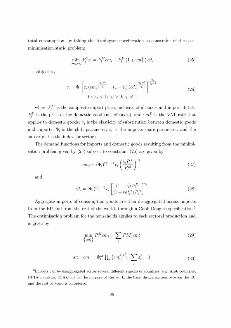
Data

For the base year 1987 data provided by the Department of Statistics (DOS) of

Jordan include the input-output table along with data on the sectoral spending for

intermediate consumption goods, sectoral data on output, exports and imports. The

input-output table Q is a square matrix - i.e. the number of activities is the same as

the number of commodities - and includes 51 economic activities.

For subsequent years (1988-2001) data on intermediate consumption, gross output,

imports and exports are available. These data are published within the revised system

of national accounts and are thus inconsistent with the sectoral classification used in

the 1987 I-O table. Revised national accounts data for 1987, i. e. data conforming

with the new classification are also available. Unfortunately, this is not the case for

the I-O table.

In order to minimise errors incurred by the change in the classification the ac-

tivities are aggregated to just nine sectors producing goods. Further, the lack of

disaggregated data for imports and exports of services implied that all eight service

sectors had also to be aggregated. This is certainly a drawback, particularly for

a country such as Jordan, where the service sector plays a very important role in

the economy and a more detailed disaggregation for services would be appropriate.

Therefore, the updated I-O matrices end up with 10 sectors, as shown in Table 2.2.

14

No.12

3.13.23.33.43.53.63.74-9

Other manufacturesServices

Manufactures of wood, paper, printingManufactures of petrolum and chemicalsManufactures of rubber and other non metallic mineralManufactures of basic metals and fabricated metal execpt machinery and equipment

Agriculture, hunting, forestry, and fishingMining and quarryingManufactures of food, beverage and tobaccoManufactures of textiles, apparels, and leather product

Economic activity

Table 2.2. DOS classification with aggregated services.

Unfortunately, both for 1987 and all subsequent years, the revised data are not

suitable to easy application of the RAS method. Three main problems were encoun-

tered.

The first problem is that variables are often evaluated at different prices, e.g.

intermediate consumption at producer prices and output at basic prices. To adjust

the data, all variables are thus evaluated at producer prices. Basic price is the price

received by the producer from the purchaser for a unit of good or service, minus

any taxes payable and plus any subsidies receivable on that unit. Producer price

is the value received by the producer for a unit of product, minus any deductible

tax (such as VAT) charged on the purchaser, but it includes non-deductible taxes

and subsidies. This requires the transformation of sectoral output evaluated at basic

prices into sectoral output at producer prices by applying the relevant net tax rate

on the basic-price output level.

A second problem faced with the data concerns the different classifications of

internationally traded goods that make figures for imports and exports of goods in-

compatible with the rest of the data. The classification used by the DOS in the orig-

inal input-output table is similar but not identical to the Harmonized System (H.S.),

which is a classification including only goods. Available external trade statistics for

goods are provided under the Brussels Tariff Nomenclature (B.T.N.) classification

for the period 1987-1993 and under the H.S. from 1994 onwards. Thus correspon-

dences must be used to convert external trade data from B.T.N. and H.S. into the

appropriate DOS classification. Some of these correspondences had to be constructed

particularly for this purpose. The appendix provides details about the concordances

used.

The third problem is certainly the major one. As explained above, application of

the RAS method requires the use of data across production sectors on total output

15

(x), domestic supply (y), and supply and demand of intermediate goods (r and c).

Whereas vectors x, y and c are known for all years, the vector of intermediate goods

supply r is known only for the base-year, i.e. 1987. The vector r needs therefore to

be derived for the remaining years. Note that data on final uses across production

sectors are not available either, so that it is impossible to compute r as the residual

from output minus final uses. Instead, the strategy used here consists in estimating

r by using sectoral data on supply and by adjusting it to make total demand for

intermediate goods in the economy equal to intermediate goods total supply.

Scalars, vectors and matrices referring to the original 1987 data are denoted with

∼ and time indices are omitted in order to keep notation simple.Define si as the ratio of ri, total intermediate input supply of sector i in 1987, to

yi, supply of sector i in 1987:

si =ri

yi(11)

Collect these intermediate production shares in the vector s:

s =

⎡⎢⎢⎢⎢⎣s1

.

.

sn

⎤⎥⎥⎥⎥⎦ (12)

The vector s is used to obtain estimates of r for each year, on the assumption that

each ri is proportional to the respective yi. The variable y is referred to as domestic

supply, not output. The reason for this is given by the fact that entries qi,j’s in the

matrix Q are domestic sales - including imports and excluding exports. Moreover,

the elements of r must be adjusted to make total supply of intermediates equal to

total demand in the intermediate goods market, i.e.P

i ri =P

i ci.

The estimate of ri for each year is therefore given by:

ri = siyi

Pj cjPj sjyj

(13)

Since the revised 1987 data differ quite substantially from the original figures, the

first step consists in updating the 1987 I-O table to the new classification. This

enables to check how strongly the change in the accounting system affects the Leontief

coefficients. In order to distinguish between the Leontief coefficients of the original

16

1987 input-output table and Leontief coefficients of the updated 1987 table (based

on revised data), the former are denoted as 1987o and the latter as 1987r. Table 2.3

below shows the original 1987 Leontief coefficients, i.e. the input-output coefficients

computed by making use of the original 1987 dataset on intermediate consumption

and gross output. By comparison, Table 2.4 shows the 1987r Leontief coefficients

obtained from applying the RAS method.

1 2 3.1 3.2 3.3 3.4 3.5 3.6 3.7 4-91 0,067 0,000 0,215 0,000 0,000 0,000 0,000 0,002 0,001 0,0032 0,000 0,118 0,000 0,000 0,000 0,048 0,041 0,002 0,004 0,005

3.1 0,167 0,000 0,122 0,007 0,003 0,001 0,001 0,001 0,000 0,0083.2 0,000 0,000 0,000 0,499 0,003 0,000 0,000 0,001 0,001 0,0013.3 0,000 0,002 0,013 0,006 0,222 0,011 0,018 0,008 0,004 0,0073.4 0,031 0,112 0,016 0,016 0,050 0,144 0,192 0,035 0,035 0,0763.5 0,010 0,002 0,012 0,010 0,002 0,007 0,056 0,014 0,206 0,0503.6 0,002 0,031 0,024 0,014 0,023 0,014 0,022 0,177 0,084 0,0453.7 0,011 0,050 0,004 0,016 0,014 0,003 0,006 0,021 0,294 0,0384-9 0,148 0,160 0,200 0,102 0,101 0,040 0,150 0,087 0,250 0,178

Table 2.3. Original 1987 Leontief coefficients

1 2 3.1 3.2 3.3 3.4 3.5 3.6 3.7 4-91 0,082 0,000 0,212 0,000 0,000 0,000 0,000 0,003 0,001 0,0032 0,000 0,100 0,000 0,000 0,000 0,068 0,037 0,004 0,002 0,004

3.1 0,196 0,000 0,115 0,004 0,004 0,002 0,001 0,001 0,000 0,0073.2 0,000 0,000 0,001 0,487 0,006 0,001 0,000 0,002 0,001 0,0023.3 0,000 0,002 0,012 0,003 0,310 0,015 0,016 0,013 0,002 0,0063.4 0,040 0,101 0,017 0,011 0,077 0,216 0,185 0,062 0,024 0,0673.5 0,015 0,003 0,014 0,007 0,003 0,013 0,063 0,029 0,159 0,0503.6 0,003 0,029 0,025 0,009 0,037 0,021 0,022 0,323 0,057 0,0403.7 0,016 0,053 0,005 0,012 0,025 0,005 0,007 0,044 0,229 0,0394-9 0,204 0,158 0,223 0,074 0,170 0,065 0,158 0,169 0,182 0,170

Table 2.4. Estimated 1987 Leontief coefficients.

Results and Conclusions

Using the RAS algorithm for all subsequent years from 1988 to 2001 allows to

analyse how the input-output coefficients change between the base-year 1987o and

over the period 1987r-2001.

In the analysis of the Leontief coefficients, it is sensible to focus on those coef-

ficients that are in some sense ”important”. While many different approaches - all

of them somehow arbitrary - to choose the level of ”importance” are available, two

reasonable criteria seem to be:

17

(i) to select those coefficients ai,j , whose value is ”large” in at least one period,

where ”large” values are those equal to or larger than 0.1;

(ii) to take those coefficients ai,j , whose associated spending for intermediate in-

puts qi,j is ”large” in at least one period, where now ”large” values are defined those

equal to or larger than 10% of total spending of sector j for intermediate consumption

goods cj in this period.

Clearly, the criterion defined in (i) identifies a subset of the coefficients identified

by criterion (ii), since (i) postulates that the value of a certain intermediate be more

than 10% of total output value, while (ii) merely postulates that it be more than 10%

of total intermediate consumption expenses of the particular sector.

Table 2.5 shows the mean values and the standard deviations (in brackets) of all

Leontief coefficients, computed over the period 1987r-2001. The coefficients whose

value is larger than 0.1 for at least one observation are shown in bold. According to

such criterion, there are 23 ”large” coefficients. Figures in italics show the coefficients

whose intermediate consumption entry is larger than 10% of total sectoral spending

for intermediates for at least one observation. Under criterion (ii), the group of ”large”

coefficients includes the same 23 coefficients selected under criterion (i), together with

additional 9 coefficients.

1 2 3.1 3.2 3.3 3.4 3.5 3.6 3.7 4-90.094 0.000 0.219 0.000 0.000 0.000 0.001 0.004 0.001 0.003(0.015) (0.000) (0.039) (0.000) (0.000) (0.000) (0.000) (0.001) (0.000) (0.001)0.000 0.080 0.000 0.000 0.000 0.076 0.031 0.003 0.002 0.003

(0.000) (0.013) (0.000) (0.000) (0.000) (0.011) (0.005) (0.001) (0.000) (0.001)0.277 0.000 0.145 0.007 0.006 0.004 0.001 0.002 0.000 0.009(0.054) (0.000) (0.017) (0.003) (0.001) (0.000) (0.000) (0.000) (0.000) (0.001)0.000 0.000 0.001 0.474 0.006 0.001 0.000 0.002 0.001 0.002

(0.000) (0.000) (0.000) (0.059) (0.002) (0.001) (0.000) (0.001) (0.000) (0.001)0.000 0.002 0.013 0.005 0.350 0.025 0.019 0.015 0.002 0.007

(0.000) (0.000) (0.001) (0.002) (0.022) (0.005) (0.002) (0.002) (0.000) (0.001)0.045 0.112 0.017 0.014 0.082 0.336 0.213 0.066 0.021 0.068

(0.011) (0.012) (0.003) (0.007) (0.009) (0.050) (0.019) (0.004) (0.002) (0.005)0.022 0.004 0.017 0.013 0.005 0.024 0.089 0.038 0.179 0.064

(0.006) (0.001) (0.004) (0.007) (0.001) (0.005) (0.014) (0.005) (0.022) (0.008)0.004 0.033 0.026 0.013 0.040 0.034 0.025 0.348 0.053 0.042

(0.001) (0.004) (0.004) (0.006) (0.005) (0.006) (0.003) (0.030) (0.005) (0.006)0.024 0.074 0.007 0.021 0.034 0.011 0.010 0.058 0.263 0.051

(0.007) (0.012) (0.001) (0.011) (0.006) (0.002) (0.002) (0.008) (0.030) (0.007)0.206 0.157 0.202 0.086 0.160 0.091 0.161 0.160 0.148 0.156(0.028) (0.020) (0.027) (0.034) (0.016) (0.012) (0.012) (0.020) (0.018) (0.018)

3.7

4-9

3.3

3.4

3.5

3.6

1

2

3.1

3.2

Table 2.5. Means and standard deviations of the coefficients

As can be seen, most of the ”large” coefficients lie along the main diagonal and

on the bottom row. This means that most of intermediate trade involves several

18

activities that buy intermediate inputs from themselves - i.e. intra-sectoral trade

between the same sector plays an important role - and sectors that buy intermediate

goods from the services sectors. More importantly, the standard deviations of all

”large” coefficients are ”small”, suggesting that the RAS procedure computed fairly

similar coefficients for all the years. This may be interpreted as an indication that

the approximations used to assemble the appropriate data and the update method in

general may have worked quite well, since, despite large swings in particular import-

export data, similar estimates have been obtained for all of the years.

In order to find out if and how much Leontief coefficients have changed over time,

the ”large” coefficients are regressed on a constant and time trend:

ai,j = α+ βt (14)

Table 2.6 shows the sign of time trends of ”large” coefficients, whose estimate of

β is significant. By looking at selected graphs depicted in appendix 1, the general

impression is that trend-induced changes in Leontief coefficients are slow and far from

dramatic. With few exceptions, time trends of Leontief coefficients are positive for in-

termediates produced by non-service sectors and negative for intermediates produced

by service sectors.

1 2 3.1 3.2 3.3 3.4 3.5 3.6 3.7 4-91 neg2

3.1 pos pos3.2 neg3.33.4 pos pos pos pos3.5 pos pos pos3.63.7 pos pos pos4-9 pos pos neg neg neg neg negTable 2.6. Time trends of the Leontief coefficient estimates.

Trending Leontief coefficients can, in principle, either reflect technological change

or changes in market structure. Technological change is different to measure, hence

one could try to explore the hypothesis that changes in Leontief coefficients are mostly

due to changes in market structure. For this purpose, data on the number of firms

in each sector are checked since an increase in a Leontief coefficient might be due

to a decrease in vertical integration and thus an increase in the number of firms in

19

a specific sector. Time-series data for the period 1990-1998 are available for sectors

2 to 3.7, whereas they are only partially available for sector 4-9, and not available

at all for sector 1. The complete dataset is shown in the appendix. After excluding

sector 1 because of lack of data and including dummies for the missing figures in

sector 4-9, the number of firms in each sector is regressed against a constant and

time. The number of firms shows significantly positive time trend over the 1990-98

period for all sectors. This can be taken as an evidence supporting the view that

vertical integration has decreased, and that competition has increased, particularly

in the manufacturing sectors.

Regressing the Leontief coefficients against a constant and the number of firms is

supposed to yield some informative and suggestive result. However, only 11 Leontief

coefficients depend significantly on the number of enterprises, as shown in table 2.7.

1 2 3.1 3.2 3.3 3.4 3.5 3.6 3.7 4-912 neg

3.1 neg3.23.33.4 pos pos pos3.5 pos pos pos3.63.74-9 pos pos pos

Table 2.7. Effects of number of firms on Leontief coefficients.

20

3 The Standard Trade Model

General equilibrium modelling approach for policy analysis has become widespread for

both developed and developing economies. In developing countries, CGE models are

commonly used for a wide range of policy issues. The policy applications range from

long-run development strategies on growth and resource allocation, to tax and trade

policy reforms. As pointed out by de Melo (1988), the issue of foreign trade policy

has occupied a center place in most of the applications. Even in the applications that

do not focus on foreign trade, the way foreign trade is modelled plays a fundamental

role in determining the outcome of policy simulations.

Over the past decades, the interest generated by computable general equilibrium

(CGE) modelling in applications to developing countries can be explained by many

factors. Firstly, the CGE modelling approach is appropriate when analysing policy

changes and external shocks that affect the whole economy. Secondly, construction of

CGE models has been facilitated by the development in many developing countries

of relevant and statistical data bases, such as social accounting matrices (SAMs).

Finally, the computational constraints on the implementation of CGE models have

been removed by advances in numerical solution techniques (Bandara, 1991).

Many general equilibrium studies have assessed the economic impacts of tariff

reform and domestic complementary policies in developing countries. Harrison et

al. (1996) assess the impacts on Turkey of a custom union arrangement with the

EU. Regional integration with the EU is found to raise welfare in Turkey between

1% and 1.5%, depending on the complementary policies adopted by the Turkish

government. By using a standard static general equilibrium, Hoekman and Konan

(1999) investigate the effects of the free trade agreement between Egypt and the EU on

Egypt’s welfare. They find large gains in welfare conditional on eliminating regulatory

barriers and red tape. In a static general equilibrium model for Syria, B. Lucke (2001)

studies different scenarios of preferential trade liberalisation with the EU, and focuses

on the effects of tariff reform on government budget. The study finds that government

revenue losses caused by reduction in the EU import duties are fairly large, but still

manageable. Go (1994) uses a model in a parsimonious and dynamic framework

to examine intertemporal effects of external shocks and adjustment policies in the

Philippines, and concludes that complementary measures, consisting of domestic tax

reform, are needed. Devarajan and Go (1998) present a similar model, and analyse the

21

response of the Philippinian economy to a terms-of-trade shock, tariff liberalisation

and fiscal policy changes. Harrison et al. (1997), using a multiregional model, find

that the implementation of the Uruguay Round has a negative impact on welfare in

countries of the MENA region.

Previous studies by Hosoe (2001) and D. Lucke (2001) on Jordan’s trade liberali-

sation implemented static models with homogenous agents and focused on aggregate

welfare and fiscal effects. Hosoe (2001) investigates the impacts of two trade pol-

icy scenarios for Jordan, the Uruguay Round implementation and the establishment

of a free trade area with the EU, by using a static model based on Devarajan et

al. (1990). Simulation of the Uruguay Round shows that its implementation would

increase Jordan’s welfare by 0.28%. The EU-Jordan FTA scenario would further in-

crease Jordan’s welfare by 0.16%. The work by D. Lucke (2001) focuses on fiscal

effects of the EU-Jordanian Association Agreement, and discusses fiscal responses

aiming at overcoming the loss in government revenue, such as simplifying and har-

monising tax rates, and broadening the tax base. However, these models do not

account for intertemporal effects due to capital accumulation.

The model implemented in this chapter is a neo-classical open-economy single-

country intertemporal model, it builds on previous work done by Feraboli et al.

(2003), which is based on the dynamic framework developed by Devarajan and Go

(1998). Discounted lifetime utility of the representative consumer is maximised by

choosing optimal consumption and investment paths. In the domestic economy there

are ten production sectors, nine of which producing goods and one producing ser-

vices. Production sectors will be denoted by the subscript i. Perfect competition

and full employment are assumed in all sectors. Firms use intermediate inputs and

value added output to produce final output with a Leontief production technology.

Value added output is in turn a constant elasticity of substituion (CES) composite of

primary inputs, capital and labour. Production factors are assumed to be perfectly

mobile across sectors. International trade flows are characterised by imperfect sub-

stitution between domestic and foreign goods. Final sectoral output Q is allocated

across domestic sales D and exports E through a constant elasticity of transformation

(CET) function. Total sectoral absorption X is an Armington (1969) composite of

domestic good D and imported good M . It is differentiated among four uses: private

consumption C, government consumption G, intermediate input q, investment I. The

parameters in the Armington functions are the same for all uses, as well as prices.

22

The domestic country is assumed to be a price-taker in the international markets,

that is world prices of imports and exports are exogenously determined.

The model is implemented by means of the mathematical software Gauss and by

employing the relaxation algorithm proposed by Trimborn (2006).

3.1 Consumers

The representative consumer chooses consumption and new capital so as to maximise

her discounted lifetime utility, subject to the budget constraint, the motion equation

of capital, the equality between savings and investment, and the given initial capital

stock. The optimisation problem is given by:

max

Z ∞

0

u (Ct) e−ρtdt (15)

subject to

K = I − δK =Y D − PCC

P I− δK (16)

K (0) = K0 (17)

where C, Y D, K are aggregate consumption, disposable income and capital of the

representative household, respectively, I is aggregate investment, PC is the composite

consumption price, P I is the composite price of investment. The household discounts

future utility with discount rate ρ, which is calibrated from the data. The depreciation

rate of capital, δ, is also calibrated from the data.

Disposable income of the representative household is given by

Y D =¡1− tY ¢ £wL+ ¡1− tK¢ rK + TR+ erFREM¤ (18)

where L is the fixed labour supply, w is the wage rate, tY is the income tax rate,

tK is the capital rent tax rate, r is the rate of return to capital, TR is government

transfer to households, FREM are foreign remittances, expressed in foreign currency,

and er is the exogenous exchange rate, which is chosen as numeraire.

The instantaneous utility function is given by the constant relative risk aversion

(CRRA) utility function:

u (C) = lnC (19)

23

which implies an elasticity of substitution between consumption at any two points

in time equal to 1.

Solving the above dynamic optimisation problem yields the Euler equation

C

C=

¡1− tY ¢ ¡1− tK¢ r

P I− ρ− δ (20)

Equations (16) and (20) characterise the dynamics of the model.

Household aggregate consumption is a Cobb-Douglas composite of consumption

sectoral goods

C = ΩCNYi=1

cθCii ; Ω

C > 0; 0 < θCi < 1 (21)

where ci is private consumption of good produced by sector i, N = 10 is the

number of sectors in the Jordanian economy, ΩC is the shift parameter and θCi is the

share parameter of good i in the Cobb-Douglas consumption function.

Solving the static problem

maxci

ΩCNYi=1

cθCii (22)

subject to the constraint

PCC =

NXi=1

PXi ci (23)

yields the functions of demand for consumption good produced by sector i

ci = θCiPCC

PXi(24)

where ci is private consumption demand for the good produced by sector i, PC is

the private consumption price index and PXi is the price of the final good produced

by sector i.

Household consumption of each good and service ci’s are in turn composites of

domestic and import goods, modelled through the Armington (1969) assumption of

constant elasticity of substitution (CES) between domestically-produced consumption

good cdi and imported consumption good cmi. The representative household chooses

the optimal level of each domestic and import good and service for a given value of

24

total consumption, by taking the Armington specification as constraint of the cost-

minimisation static problem:

mincmi,cdi

PCi ci = PMi cmi + P

Di

¡1 + vatDi

¢cdi (25)

subject to

ci = Φi

∙εi (cmi)

γi−1γi + (1− εi) (cdi)

γi−1γi

¸ γiγi−1

0 < εi < 1; γi > 0, γi 6= 1(26)

where PMi is the composite import price, inclusive of all taxes and import duties,

PDi is the price of the domestic good (net of taxes), and vatDi is the VAT rate that

applies to domestic goods; γi is the elasticity of substitution between domestic goods

and imports, Φi is the shift parameter, εi is the imports share parameter, and the

subscript i is the index for sectors.

The demand functions for imports and domestic goods resulting from the minimi-

sation problem given by (25) subject to constraint (26) are given by

cmi = (Φi)(γi−1) ci

µεiP

Xi

PMi

¶γi

(27)

and

cdi = (Φi)(γi−1) ci

∙(1− εi)P

Xi

(1 + vatDi )PDi

¸γi(28)

Aggregate imports of consumption goods are then disaggregated across imports

from the EU and from the rest of the world, through a Cobb-Douglas specification.3

The optimisation problem for the households applies to each sectoral production and

is given by:

mincmj

iPMi cmi =

Xj

PMji cm

ji (29)

s.t. cmi = ΦMiQj

¡cm

ji

¢εji ; Xj

εji = 1 (30)

3Imports can be disaggregated across several different regions or countries (e.g. Arab countries,

EFTA countries, USA), but for the purpose of this work, the basic disaggregation between the EU

and the rest of world is considered.

25

where cmji is households consumption of foreign good i imported from region j,

PMji is the price of good i imported from region j inclusive of all taxes, ΦMi is the

shift parameter, and εji is the share parameter of imports of good i from region j, with

each εji ≥ 0. The elasticity of substitution between imports is therefore constant and

equal to one, being the Cobb-Douglas specification a particular case of CES function.

The solution to the above minimisation problem yields the demand functions for

imports disaggregated across foreign regions:

cmji = ε

ji

PMi cmi

PMji

; i = 1, 2, .., N ; j = EU,RW (31)

The domestic prices of imported goods are determined exogenously, since they

depend on the fixed world price of imports, PWMi , the import tariff rate, tm

ji , the

VAT rate on imported goods, vatMi , and the exchange rate er:

PMji = erPW

Mi

¡1 + tm

ji

¢ ¡1 + vatMi

¢; j = EU,RW (32)

3.2 Firms

On the supply side, constant returns to scale and perfect competition are assumed.

Sectoral output in the domestic economy Qi is determined by a two-stage production

technology, which exhibits at the top tier a Leontief fixed-proportions specification

between intermediate input qj,i produced by sector j and used in the production

process of sector i, and value-added output V Ai:

Qi = min

½V Ai

a0,i,qj,i

aj,i, ....

¾(33)

where a0,i is the fixed requirements of valued-added output V Ai, and aj,i is the

fixed requirements of intermediate input qj,i for production of aggregate output Qi.

At the second tier, intermediate input qj,i is an Armington CES composite of

domestic and foreign intermediate consumption goods, qdj,i and qmj,i. Total import

of intermediate goods is in turn a Cobb-Douglas composite of intermediate input

regional imports.

Value-added production in each sector i is determined by a technology charac-

terised by a constant elasticity of substitution between the two primary inputs, capital

26

and labour, which are perfectly mobile across sectors:

V Ai = Ai

"αiLD

σi−1σi

i + (1− αi)KD

σi−1σi

i

# σiσi−1

0 < αi < 1; σi > 0; σi 6= 1(34)

where LDi and KDi are sector i’s demand for labour and capital respectively,Ai

is a time-invariant technological parameter, αi is the labour share parameter and σi

is the constant elasticity of substitution between labour and capital.

At the value-added production stage, subject to the above technology constraint

(34), firms minimise production costs, given by

P V Ai V Ai = wLDi + rKDi (35)

where P V Ai is the value-added price, w is the nominal wage rate and r is the

nominal rate of return to capital.

Cost-minimisation subject to the technology constraint yields the demands for

labour and capital

LDi = (Ai)(σi−1) V Ai

µαiP

V Ai

w

¶σi

(36)

KDi = (Ai)(σi−1) V Ai

∙(1− αi)P

V Ai

r

¸σi(37)

Sectoral production Qi can be sold on the domestic market or abroad. Exports

and domestic sales are modelled according to a constant elasticity of transformation

(CET) function, that represents the constraint for the producer maximising total

sales:

maxEi,DS

i

PQi Qi = P

Ei Ei + P

Di Di (38)

s.t. Qi = χi

"θiE

1+ΨiΨi

i + (1− θi)D

1+ΨiΨi

i

# Ψi1+Ψi

(39)

where Qi is total sectoral domestic production, Ei is exports, Di is domestic

supply, PQi is producer output price (i.e. net of taxes), P

Ei is producer exports price

27

(which turns to be equal to the world price of exports PWEi , given the absence of

export subsidy), PDi is producer domestic sales price (i.e. net of VAT), θi is the export

share parameter, χi is the shift parameter, and Ψi is the elasticity of transformation

between domestic good and export good, with 0 < θi < 1, χi > 0 and Ψi > 0.

Solving the above maximisation problem yields the following supply functions of

domestically-sold and exported goods

Di =Qi

(χi)(1+Ψi)

³PQi

´Ψi µ PDi1− λi

¶Ψi

(40)

Ei =Qi

(χi)(1+Ψi)

³PQi

´Ψi µPEiλi¶Ψi

(41)

Total exports are allocated across the EU and the rest of the world by means of

the optimisation problem, in which, as above, a constant elasticity of transformation

(CET) specification is adopted:

maxEji

PEi Ei =Xj

PEjiE

ji (42)

s.t. Ei = χEi

"Pj

θji

¡Eji

¢1+ψEiψEi

# ψEi1+ψEi

;Xj

θji = 1 for j = EU,RW

(43)

where total sectoral exports Ei is a composite of regional exports EEUi and ERWi ,

PEji are producer export prices (all of them equal to the fixed world price of exports,

PWEi ), χ

Ei > 0 is the shift parameter, θ

ji is the share parameter of exports to region

j = EU,RW , ψEi is the elasticity of transformation between exports, with ψEi > 0,

and PEji is the producer price of exports to region j.

The supply functions of exports to each foreign region j produced by sector i are

given by

Eji =

Ei

(PEi )ΨEi (χEi )

(1+ΨEi )

ÃPE

ji

λji

!ΨE

; i = 1, 2, , .., N ; j = EU,RW (44)

Prices of the export good, produced by sector i and exported to region j are equal

to exogenous and fixed world export prices times the exchange rate:

PEji = erPW

Ei ; j = EU,RW (45)

28

Aggregate investment I is a Cobb-Douglas composite of sectoral investment goods,

invi. Each sectoral investment good invi is characterised by a CES Armington speci-

fication between investment domestic goods invdi and total imports invmi, and by a

Cobb-Douglas function for disaggregated imports. Given that functional parameters

and prices are the same for all kinds of uses, optimal investment is determined in the

same fashion as (25)-(31).

3.3 Government

The government consumes an exogenous amount of goods, raises taxes and tariffs,

provides a transfer to consumers, and runs a balanced budget. Although at first sight

the assumption of balanced budget might look unrealistic, it is actually appropriate

and roughly consistent with government fiscal balance data for Jordan provided by

the IMF.4

Aggregate government consumption G is a Cobb-Douglas composite of sectoral

goods gi. In turn, each government sectoral consumption is determined by a CES

Armington specification between domestically-produced goods gdi and imports gmi

in the same way as in (25)-(31). Government revenue is generated from the Value

Added Tax (VAT), that applies with different rates to domestic and imported goods

(vatd and vatm), the tax on capital rent (tK), the income tax (tY ), import duties,

that apply with different rates to the EU and the rest of the world (tm), and foreign

grants, FRG, expressed in foreign currency. The expenditure is given by transfer to

household TR, and consumption of good G.

The government budget is therefore given by

V ATD + V ATM + TY + TK + TM + erFRG = TR+G (46)

where V ATD is revenue of VAT on domestic goods, V ATM is revenue of VAT on

imports, TY is income tax revenue, TK is revenue of tax on capital rent, and TM is

import tariff revenue.

4The IMF reported the Jordan’s government fiscal balance in percent of GDP to equal -4.9 in

2002, -1.0 in 2003 and -1.7 in 2004 (see IMF, 2006).

29

3.4 Market clearing

The equilibrium on the factors markets requires aggregate endowment of labour be

equal to aggregate labour demand and aggregate capital stock be equal to aggregate

demand for capital

L =

NXj=1

LDj (47)

K =

NXj=1

KDj (48)

where L is labour supply (fixed), K is aggregate capital stock, and LDj and KDj

are demands for labour and capital of production sector j.

The equilibrium in the domestic good markets is given by

Xi =

NXj=1

qi,j + ci + invi + gi (49)

where Xi is total sectoral absorption,NPj=1

qj,i is total intermediate inputs produc-

tion, ci is private consumption, invi is investment demand, and gi is government

consumption, in sector i.

The equilibrium in the balance of payments is given by

NXi=1

PWMi Mi =

NXi=1

PWEi Ei + FREM + FGR (50)

where Mi and Ei are, respectively, total imports and total exports of sector i,

PWMi and PWE

i are the exogenous world prices of, respectively, imports and exports

of sector i, FGR is foreign grant to the Jordanian government, and FREM are

foreign remittances to households.

3.5 Data and calibration

The dataset is based on the Social Accounting Matrix (SAM) for Jordan constructed

by D. Lucke (2001). The SAM is based on 1998 data, and includes the 1987 input-

output coefficient matrix updated to 1998. The SAM has nine sectors producing

goods and one sector producing services.

30

The model described in the above section has been initially applied in a simplified

version with only two production sectors, producing respectively goods and services.

Later, as shown in the set of simulations below, the size of the model has been enlarged

to include the original 1998 SAM with ten sectors, listed in Table 3.1.

The base-year dataset is assumed to reflect a stationary steady state economy. Pa-

rameters are then calibrated in order to obtain a solution reproducing the benchmark

equilibrium.

No. Economic activity1 Agriculture, hunting, forestry and fishing2 Mining and quarrying

3.1 Manufactures of food, beverage and tobacco3.2 Manufactures of textiles, apparels and leather product3.3 Manufactures of wood, paper and printing3.4 Manufactures of petroleum and chemicals3.5 Manufactures of rubber and other non-metallic minerals3.6 Manufactures of basic metals and fabricated metal except machinery and equipment3.7 Other manufactures4-9 Services

Table 3.1. Production sectors.

The world prices of export PWEi and import PW

Mi are exogenously fixed to one.

Real variables are then derived from the base-year nominal variables provided in the

SAM. Elasticity values are taken from existing literature, as Table 3.2 shows.

Elasticity Value Source

Substitution between domestic goods and imports 0.6 Devarajan et al. (1999)

Transformation between domestic goods and exports 1.5 Devarajan et al. (1997)

Transformation between regional exports 3 Martin (2000); Lucke B. (2001)

Substitution between labour and capital 0.9 Devarajan and Go (1998)Table 3.2. Elasticity values.

The assumption of steady state allows to calibrate the dynamic parameters δ and

ρ. From the capital accumulation equation (16) and from the stationary steady-state

condition Kt = Kss, it follows that the depreciation rate of capital is:

δ =Iss

Kss

(51)

where the subscript ss indicates steady state.

31

The steady-state intertemporal condition for private consumption, given by the

Euler equation (20), allows then to calibrate the consumers’ discount rate as:

ρ =¡1− tY ¢ ¡1− tK¢ rss

P Iss− δ (52)

The steady-state conditions apply also as terminal conditions.

3.6 Simulations

The basic feature of each scenario, exogenous and common to all simulations, is given

by the gradual reduction of tariff rates on EU-import goods, provided by the EU-

Jordan Agreement, and described in table 3.3. For agricultural goods and industrial

goods containing agricultural components the import duty reduction is only partial,

whereas it is complete for the remaining industrial goods.

Agriculture Mining Food Textile Paper Chemicals Minerals Metals OthersEntry into force of the AA 100% 60% 100% 60% 60% 60% 60% 60% 60%

One year after 100% 53% 100% 53% 53% 53% 53% 53% 53%Two years after 100% 47% 100% 47% 47% 47% 47% 47% 47%Three years after 100% 40% 100% 40% 40% 40% 40% 40% 40%Four years after 90% 30% 90% 30% 30% 30% 30% 30% 30%Five years after 80% 27% 80% 27% 27% 27% 27% 27% 27%Six years after 70% 23% 70% 23% 23% 23% 23% 23% 23%

Seven years after 60% 20% 60% 20% 20% 20% 20% 20% 20%Eight years after 50% 17% 50% 17% 17% 17% 17% 17% 17%Nine years after 50% 13% 50% 13% 13% 13% 13% 13% 13%Ten years after 50% 10% 50% 10% 10% 10% 10% 10% 10%11 years after 50% 7% 50% 7% 7% 7% 7% 7% 7%12 years after 50% 0% 50% 0% 0% 0% 0% 0% 0%

Table 3.3. Import tariff reduction schedule (percent of the base-year tariffs).

The immediate effect of a reduction in custom duties on imports of a specific

trade partner can be seen by considering the first-order conditions for the Armington

specification between imports and domestically-produced goods:5

cm

cd=

∙εPD

(1− ε)PM

¸γ(53)

and the first-order conditions for the Cobb-Douglas regional imports:

cmEU

cmRW=

εEUPMRW

εRWPMEU(54)

5For convenience, the subscript denoting the production sector has been dropped.

32

Prices of regional imports are defined as:

PM j = erPWM¡1 + tmj

¢ ¡1 + vatM

¢(55)

where tmj is the tariff rate on goods imported from region j and vatM is the VAT

rate applied to imports.

From (55), a decrease in tmEU will clearly reduce PMEU . From (54) it follows

that, ceteris paribus, regional import demand cmj is decreasing in the regional import

price PM j . Moreover, since PM is a composite of PMEU and PMEU , a fall in one

regional import prices will decrease PM . Therefore, a reduction in the tariff rate on

EU import will determine a fall in the EU imports price and in the composite imports

price, and a rise in EU imports.

The gradual reduction of the import duty rate decreases prices of imported goods.

Domestic prices will also decrease. The fall in domestic prices boosts directly demand,

investment might go up and output is expected to increase in the long-run. The loss

in government revenue due to the import duty reduction might be partially offset

by the expansion in the tax base in the longer run. However, the government must

compensate the fall in revenue by undertaking counteracting fiscal measures, such

as an increase in the domestic tax rates or a reduction in spending. Therefore the

simulation of the AA is accompanied by a parallel change in the domestic policy.

Moreover, some intersectoral impact is expected. The sector in which tariff reduction

is complete is likely to attract more resources in the long-run, although it might suffer

from a short-run negative impact due to the move from protectionism to free trade.

The impact on welfare might be in principle ambiguous. On the one hand, lower

domestic prices increase consumption and hence households’ welfare. On the other

hand, the reduction in government revenue due to cutting import duty rates forces

the government to implement painful fiscal measures, such as increase in domestic

tax rates or reduction in transfer to households. This will negatively affect disposable

income of households, who must ceteris paribus reduce consumption. Such an impact

on welfare is therefore negative. The overall impact on households’ consumption

and welfare depends therefore on the magnitude of the effects of lower consumption

prices and lower disposable income. However, the simulations results show that under

all scenarios of trade liberalisation welfare rises. Table 3.4 lists the scenarios and

summarises the welfare effects.

33

Scenario Policy variables Welfare change %1 Government transfer 0,062 Income tax rate 0,033 Government consumption 0,164 Government transfer; VAT 10% increase 0,035 Government consumption; VAT 10% increase 0,07

Table 3.4. Scenarios and welfare changes.

All scenarios are characterised by two-policy simulations. Trade policy is deter-

mined exogenously, it is established by the Association Agreement with the EU and is

common to all scenarios, while the responses of domestic policy are a mix of endoge-

nous and exogenous options. In scenario 1, government transfer to households is the

endogenous policy variable. In scenario 2, the reform of the domestic income taxation

is the government endogenous policy choice. In the third scenario, the endogenous

policy choice is government consumption. In scenarios 4 and 5, respectively gov-

ernment transfer and government consumption are endogenous, while an additional

exogenous policy response is put into effect in both scenarios, namely an increase by

10% in the VAT rates.

Scenario 1: Association Agreement and endogenous government trans-

fer

As pointed out above, the reduction of the import duty rates on EU imports

will immediately decrease the prices of imported goods. This will cause, ceteris

paribus, a fall of final internal prices, which are a composite of prices of imports

and domestically-produced commodities. As figure 3.1 shows, composite prices of

private consumption (PC), government consumption (PG) and investment (PI) fall

relatively to their benchmark levels, which have been initialised to one, and approach

the new steady-state level from above.

Alongside the exogenous import duties reduction, the endogenous policy variable

playing a role in the simulation is government transfer to households. Clearly, given

the fall in government revenue, transfer to households is expected to decrease. As

shown in figure 3.2, during the gradual reduction of the EU import tariff rates, the

drop in government revenue forces the government to cut transfer to households,

which falls relatively to the benchmark value equal to one, has a decreasing trend

until the 13th year, increases very slightly and finally approaches the steady state

from below.

34

0,975

0,98

0,985

0,99

0,995

1

1,005

time

PC PI PG

Figure 3.1. Prices under scenario 1.

The path of transfer in the initial 15 years shows ups and downs. This rather

unexpected time path characterises also the trend of government revenue, shown in

figure 3.3. This is due to the fact that, whereas time is continuous, the import tariff

reduction is a discrete-time process, i.e. it takes place at a specific point in time.

This causes a discrete adjustment in government revenue, that fluctuates around the

trend. The behaviour of government revenue in turn affects the path of transfer to

households.

0,6

0,65

0,7

0,75

0,8

0,85

0,9

time

Figure 3.2. Government transfer to households under scenario 1.

The implementation of this two-policy simulation has two impacts on the revenue

of government: (i) an immediate and direct effect brought about by the reduction in

35

import duties, that lowers government revenue; (ii) the expected effect of increased

internal demand, determining a larger domestic tax base, that raises government

revenue.

The outcome depends on the magnitudes of the above two effects. Altogether

the first effect is larger, as both government revenue and transfer to households are,

for all time periods, below their benchmark values. However, along the transition

to the new steady state, it might well be that in some periods the second effect

is larger than the first one, and thereby government revenue and transfer increase

relatively to the previous time period. In fact, after the negative trend in the initial

periods, government revenue increases slightly and approaches the steady-state level

from below.

0,94

0,945

0,95

0,955

0,96

0,965

0,97

0,975

0,98

0,985

time

Figure 3.3. Government revenue under scenario 1.

One of the most important and most relevant results of the simulation concerns

the impact on private real consumption, since welfare of households depends on con-

sumption. As figure 3.4 shows, private consumption reaches in the long-run a higher

level than the initial benchmark value. However, although the impact on welfare is

positive, consumption initially falls relatively to the benchmark level, afterwards it

keeps increasing in all periods, and it is below the benchmark value until the 8th year

after the entry into force of the AA. The implication of this analysis suggests that

consumers must give up some current consumption in order to achieve higher future

consumption.

This clearly raises the question concerning the political feasibility of the trade

liberalisation process undertaken by the Jordanian government.

36

0 ,97

0 ,98

0 ,99

1

1 ,01

1 ,02

1 ,03

tim e

Figure 3.4. Private consumption under scenario 1.

Whereas opening up domestic trade leads unambiguously to an increase in welfare,

the government willingness to follow consistently a trade liberalisation policy might

be harmed, given the ”political price” to be paid in terms of short-run decrease in

private consumption.

Capital and investment are in all periods above their benchmark levels. The fall

in domestic prices pushes up internal demand, which, in turn, boosts new capital

formation. As shown by figures 3.5 and 3.6, capital keeps increasing and reaches the

new long-run equilibrium value from below, whereas investment follows a different

pattern. Aggregate investment is much above the benchmark value in the initial

periods, then it falls slowly, and finally reaches from above the new steady state,

which is higher than the initial level.

0,99

1

1,01

1,02

1,03

1,04

1,05

1,06

tim e

Figure 3.5. Capital stock in scenario 1.

37

1

1,02

1,04

1,06

1,08

1,1

1,12

1,14

tim e

Figure 3.6. Investment in scenario 1.

Trade liberalisation is expected to have also sectoral effects. The formerly pro-

tected sectors might experience a long-run increase in output, due to a shift of re-

sources from other sectors. However, they may be negatively affected in the very

short-run, due to increased foreign competition.

0,97

1,02

1,07

1,12

1,17

time

Agriculture Mining Food Textiles PaperChemicals Minerals Metals Others Services

Figure 3.7. Sectoral outputs under scenario 1.

Nevertheless, simulation results support the view that trade liberalisation brings

about positive effects also in the short-run, and penalises sectors in which trade

openness is incomplete, i.e. agriculture and food sectors, in terms of slowdown in the

very short-run and lower long-run equilibrium levels.

Figure 3.7 shows how outputs of all good sectors are affected by opening up

domestic trade. The agriculture and food sectors, in which trade liberalisation begins

38

four years after the entry into force of the Association Agreement and in which tariff

rates are only partially reduced, experience initially a slowdown in production, and

the lowest percentage increases in the final steady-state values. Sectors in which trade

liberalisation is complete and faster avoid the short-run negative impact on output

and achieve higher long-run equilibrium levels.

Table 3.5 lists the output level for each sector at the period when the Association

Agreement enters into force, i.e. when the first shock occurs, and the steady-state

values in the long-run equilibrium. From both figure 3.7 and table 3.5 it can be seen

that agriculture and food sectors are those that benefit least from trade liberalisation,

and are actually harmed in the short-run. The same conclusion on sectoral outputs

effects can be drawn by analysing results of the remaining scenarios.

Sector first shock final steady stateAgriculture 0,9796 1,0201Mining 1,0035 1,0500Food 0,9801 1,0196Textile 1,0313 1,1751Paper 1,0210 1,0400Chemicals 1,0032 1,0565Minerals 0,9981 1,0249Metals 1,0149 1,0347Others 1,0467 1,1367Services 0,9992 1,0138

Table 3.5. Sectoral outputs.

Scenario 2: Association Agreement and endogenous income tax rate

Under this scenario the income tax rate is the endogenous policy variable used

by the Jordanian government to counteract the fall in revenue. Given the immediate

decrease in government revenue, the endogenous income tax rate is expected to be set

above the benchmark value of of 0.072, to keep increasing during the 12-year transition

period towards the free-trade area, and finally to stabilise or perhaps slightly fall,

given the possibly larger domestic tax base.

In the simulation the ”optimal” income tax rate moves to a value around 0.08 in

the initial periods, it increases steadily, after 12 years it decreases very slighly, and

it approaches from above the new steady-state rate of 0.089, as shown in figure 3.8.

Although this is a simplification, since in reality the income tax rates are six, the

simulation provides a clear and expected insight for fiscal policy reform.

39

0,07

0,075

0,08

0,085

0,09

0,095

tim e

Figure 3.8. Optimal income tax rate.

Qualitative results for all macroeconomic variables are the same like under the

other scenarios. Figure 3.9 shows the time path of capital, which is very similar

under all scenarios. Given the fall in domestic prices, investment demand goes up,

capital stock rises over time and approaches the new steady-state level from below. It

has to be noticed that the new steady-state level of capital is 1.02, which is lower than

the steady-state value of 1.05 under scenarios 1 and 3. This difference is probably

due to the distortionary effect introduced by the endogenous income tax rate. The

higher income tax rate has a negative effect on consumers’ income, and it also creates

a distortion in the optimal choices of consumers. In this simulation therefore, optimal

investment choice might be negatively affected by the endogenous income tax rate,

which is not present in the other scenarios, since tY is constant there. Due to such

distortion, ceteris paribus, capital grows less than under the other scenarios, and

reaches a lower long-run equilibrium value.

0 ,9 9 5

1

1 ,0 0 5

1 ,0 1

1 ,0 1 5

1 ,0 2

1 ,0 2 5

tim e

Figure 3.9. Capital stock under scenario 2.

40

Scenario 3: Association Agreement and endogenous government con-

sumption

In this simulation, macroeconomic variables follow a path which is qualitatively

the same as in scenarios 1 and 2. Quantitavely, it has to be noticed that the increase

in welfare is larger than under the other two scenarios, due to a faster and higher

growth in private consumption, as shown in figure 3.10.

It is in fact no surprise to find that welfare increase under scenario 3 is larger than

under the other two simulations. In the previous two scenarios the policy choice im-

plemented by the government reduces household income. Therefore, ceteris paribus,

private consumption and utility will also fall. The reduction in government con-

sumption, instead, does not reduce welfare, because government spending plays no

role in utility of consumers. However, the credibility of such result might be ques-

tioned, given that the govenrment is likely to face a problem of feasibility in cutting

consumption.

0,99

1

1,01

1,02

1,03

1,04

1,05

tim e

Figure 3.10. Private consumption in scenario 3.

Under scenarios 1 and 2, households’ consumption reaches the benchmark value

of 1 between 6 and 7 years after the start of the tariff reform, and ends with long-run

equilibrium levels which are 1.01 in scenario 3 and 1.02 in scenario 1. Without the

negative impact on income due to lower government transfer and higher income tax

rate, consumption under scenario 3 reaches the benchmark level after 2 years and

ends with a new steday-state value very close to 1.04.

The endogenous policy variable, i.e. government consumption, is expected to fall

relatively to the benchmark value of one, to keep falling given the government budget

41

constraint, and perhaps increase slightly in the long-run, when the negative short-run

effect of trade liberalisation on government revenue is compensated by the positive

effect brough about by the larger domestic tax base.

0,95

0,955

0,96

0,965

0,97

0,975

0,98

0,985

tim e

Figure 3.11. Endogenous government consumption.

Figure 3.11 depicts the dynamic path of endogenously-determined government

consumption, that lies always below the benchmark level, falls in the initial periods,

follows an increasing trend after 12 years, and finally approaches the new steady state

from below.

Scenario 4: Association Agreement, endogenous government transfer

and exogenous VAT rates increase

This scenario implements an exogenous increase in the VAT rates by 10% together

with the endogenisation of government transfer to households, like in scenario 1.

One would expect a positive impact on household welfare, brought about by trade

liberalisation. Moreover, the increase in welfare is expected to be smaller than under

scenario 1, given that the reduction of distortionary import tariffs is accompanied by

distortionary side-effects brought about by the exogenous increase in the VAT rates.

The results are consistent with expectations. Welfare rises by 0.03%, whereas under

scenario 1 the increase was 0.06%. Consumption follows a slighlty different path from

the one under scenario 1. As figure 3.12 shows, private consumption initially falls

below the benchmark value, but the initial decrease relative to the benchmark level

is smaller than the drop under scenario 1.

Private consumption rises afterwards, it reaches the benchmark level after 10 years,

and then approaches the final steady-state value from below. After normalising the

42

benchmark level to 1, the long-run equilibrium value of consumption is 1.012, smaller

than the long-run consumption under scenario 1, which is equal to 1.021. As pointed

out above, this can be explained by the effects due to the VAT rates increase.

0 ,985

0,99

0 ,995

1

1 ,005

1,01

1 ,015

tim e

Figure 3.12. Consumption under scenario 4.

There are two impacts on the consumption price index brought about by exoge-

nous policy choices. The reduction in import duties determines a decline in domestic

prices, which raises demand. On the other hand, the increase in the VAT rates brings

about a rise in prices, which has a negative impact on consumption. The consumption

price index has quite a different behaviour than the one observed under scenario 1,

as figure 3.13 shows.

0 ,9 9

0 ,9 9 2

0 ,9 9 4

0 ,9 9 6

0 ,9 9 8

1

1 ,0 0 2

tim e

Figure 3.13. Consumption price index under scenario 4.

43

Whereas previously the consumption price was below the benchmark value for all

periods, under scenario 4, it increases slightly in the initial periods, it drops along the

transition period, and then it approaches the long-run value from above. The final

steady-state price is 0.992, higher than the long-run price under scenario 1, which

was 0.982.

The exogenous increase in the VAT rates, compared with scenario 1, reduces

aggregate demand and hence also investment demand. This determines therefore a

lower growth rate of the capital stock, which reaches the long-run equilibrium level

of 1.032, as shown in figure 3.14, whereas under scenario 1 this was 1.05.

0,99 5

1

1,00 5

1,0 1

1 ,01 5

1,0 2

1 ,02 5

1,0 3

1 ,03 5

tim e

Figure 3.14. Capital stock under scenario 4.

Finally, it is worthwhile to note that, whereas under scenario 1, the burden of the

fall in government revenue was borne only by transfer to households, under scenario 4

the increase in the VAT rates determines, ceteris paribus, higher values of government

transfer. As shown in figure 3.15, transfer to households is above the benchmark value

in the initial three years and falls steadily afterwards. The long-run equilibrium value

is 0.87, fairly above the steady-state value under scenario 1, equal to 0.74.

44

0 ,8

0 ,8 5

0 ,9

0 ,9 5

1

1 ,0 5

1 ,1

tim e

Figure 3.15. Government transfer to households under scenario 4.

Scenario 5: Association Agreement, endogenous government consump-

tion and exogenous VAT rates increase

In this scenario the simulation performed in scenario 3 is extended, by adding

an exogenous ten-percent increase in the VAT rates to the endogenous change in

government consumption. Like in scenario 4, domestic prices are affected through

two exogenous channels. The gradual reduction in import tariff rates leads to lower

prices in the domestic economy, which boosts internal demand. On the other hand,

the increase in the VAT rates increases domestic prices and hence affects negatively

domestic demand. As a result, the consumption price index is at the very beginning

of the time-horizon above the benchmark value when preferential trade liberalisation

and the VAT rate increase take place, as it is shown in figure 3.16. The price index

falls thereafter, it reaches the benchmark level at the second year, and approaches

the long-run equilibrium value, equal to 0.992, from above. As expected, the final

steady-state consumption price is higher than under scenario 3, given the additional

effect brought about by the increase in the VAT rates.

Like in the other scenarios, private consumption drops below the benchmark level,

it rises steadily and approaches the final long-run equilibrium from below. The final

steady-state level of private consumption is 1.021, far below the long-run consumption

value determined by scenario 3. As a result, implementing the exogenous increase in

the VAT rates has decreased the welfare gain under scenario 3 from 0.16% to 0.07%.

45

0 ,9 9

0 ,9 9 2

0 ,9 9 4

0 ,9 9 6

0 ,9 9 8

1

1 ,0 0 2

tim e

Figure 3.16. Consumption price index under scenario 5.

Comparing these simulation results with those of scenario 3, the exogenous in-

crease in the VAT rates determines also higher government consumption, as one

would expect. As figure 3.17 shows, government consumption is above its benchmark

value in the first two periods, it then drops, overshoots and reaches the long-run

equilibrium equal to 0.98, whereas it was 0.96 under scenario 3.

0 ,9 7

0 ,9 7 5

0 ,9 8

0 ,9 8 5

0 ,9 9

0 ,9 9 5

1

1 ,0 0 5

1 ,0 1

tim e

Figure 3.17. Government consumption under scenario 5.

3.7 Conclusions

In this chapter the bilateral trade liberalisation process undertaken by Jordan has

been assessed by means of a dynamic CGE model, in which one representative con-

sumer chooses consumption and new capital in order to maximise her discounted

46

lifetime utility. The standard trade model is able to capture intertemporal effects on

Jordan of opening up domestic trade, with particular emphasis on consumer welfare.

The policy implications for the Jordanian economy of the PTA with the EU have also

been analysed.

The main conclusions drawn from the set of two-policy simulations are therefore:

(i) the Association Agreement with the EU brings about in Jordan positive long-run

effects on all macroeconomic variables; (ii) the impact of trade liberalisation on wel-

fare is positive under all scenarios; (iii) the government should counteract the negative

impact of opening up domestic trade on government revenue by implementing fiscal

policy reforms; (iv) trade liberalisation and government counteracting actions affect

negatively private consumption in the short-run and raise concerns about political

feasibility of the trade liberalisation process; and (v) sectors in which trade liberal-

isation is complete and faster benefit more than sectors in which import duties are

only partially removed.

47

4 The Poverty Model

Trade liberalisation processes undertaken by many developing countries over the past

years have raised many concerns that liberalisation of domestic trade in the developing

countries will affect negatively the poor and it will increase the income gap between

the rich and the poor. Given the lack of studies about effects of trade liberalisation

on poverty and income distribution in Jordan, this dissertation aims at providing

evidence that trade liberalisation has different impacts across different household

classes. The process of opening up domestic trade might lead to unequal distribution

of welfare gains, and might even make some specific groups worse off.

As mentioned in chapter 1, in the context of general equilibrium modelling sev-

eral studies have been conducted to assess aspects of income distribution related to

trade liberalisation (see Reimer, 2002 for a survey and Winters et al., 2004 for an

overview). However, this is the first approach that analyses income distribution in an

applied dynamic neoclassical general equilibrium framework in which heterogeneous

households are assumed to have different discount rates.

In the general equilibrium analysis of poverty and distribution issues, there are

mainly two approaches. One is to use a CGE model with one single representa-

tive consumer. The changes in commodity and factor prices generated by a trade

liberalisation experiment are applied to household data to compute the impacts on

poverty and income distribution. This approach has been followed, among others,

by Ianchovichina et al. (2001), who simulate unilateral trade liberalisation in Mex-

ico and estimate that, combining price and income changes, welfare increases for all

households, with larger proportionate changes for poorer households, and by Hertel

et al. (2001), who examine the effects of multilateral liberalisation on seven countries

and find that liberalisation reduces poverty in four countries and increases it in three

countries.

The second approach is to embed the household dissaggregation within the CGE

model. As pointed out by Winters et al., this approach has the advantage of be-

ing internally consistent. Simulations help therefore to identify the household classes

that are vulnerable even when trade liberalisation is beneficial on average. All studies

find that trade liberalisation has different impacts on different household categories.

Decaluwe et al. (1999) incorporate the analysis of income distribution and poverty

into the social accounting matrix (SAM) and computable general equilibrium (CGE)

48

methodology in an archetype African economy, characterised by six different house-

hold categories. Bourguignon at el. (1991) carry out illustrative simulations of a

stabilisation package for a representative economy, and find a large adverse impact

on the distribution of income. Harrison et al. (2003) develop a multi-regional and

multi-sectoral model to evaluate the trade policies options faced by Brazil, i.e. re-

gional arrangements and multilateral trade liberalisation. Households are disaggre-

gated across 20 groups, ten rural and ten urban, that are distinguished by income

levels. The simulations suggest that most of the trade policies options result in an

overall welfare gain to Brazil, and in larger gains to the poorest households. Cock-

burn (2001) applies a CGE model to study the impacts of Nepal’s trade liberalisation

on poverty and income ditribution. Poverty falls urban areas and increases in rural

areas. Impacts are larger with higher income levels, leading therefore to an increase

in income inequality. Lofgren (2001) studies the impact of alternative development

strategies on growth and poverty in a dynamic model for Egypt. Households are

disaggregated into six groups, according to their income, i.e. rich, middle and poor,

and the area where they live, i.e. urban and rural. He finds positive impacts of price

liberalisation on welfare of all household groups. However, the effects are smaller

for the poor, and inequality increases. The same kind of household disaggregation is

applied in a dynamic framework by Lofgren et al. (1999), who assess the effects of the

Association Agreement with the EU on Morocco. Simulation results show that trade

liberalisation has small aggregate effects, but disfavours the rural poor. However,

trade liberalisation combined with complementary domestic policies lead to welfare

increases for all household groups. Bautista et al. (1998) stress the importance of

implementing fiscal adjustment measures that accompany the process of trade liber-

alisation, and conclude that failure to undertake complementary policies may explain

why trade liberalisation efforts in many African countries did not contributed to egal-

itarian growth.

As mentioned in chapter 3, previous studies on Jordan’s trade liberalisation by

B. Lucke (2001) and Hosoe (2001) used static CGE models with one homogeneous

household. To my knowledge, there is no work on Jordan’s trade liberalisation based

on a dynamic CGE model with heterogeneous households.

The Jordanian economy is modelled as a dynamic small open economy building on

a model which is very similar to the one presented in the previous chapter. The main

difference lies on the consumption side. Whereas in the standard trade model one

49

representative household maximises her discounted lifetime utility, the poverty model

captures household heterogeneity. The household disaggregation is embedded within

the CGE model. In detail, households are disaggregated into six different classes

ranked by their disposable income. Within each of six different household groups

one typical consumer maximizes discounted intertemporal utility subject to a budget

constraint. Households groups’ individual tax rates, wage rates, initial endowments

of assets, tranfers from the government and from abroad and consumption prefer-

ences are calibrated from data from a 2002 households survey. Moreover, different

households’ time preferences are also calibrated from survey data by assuming that

consumption levels of all households are stationary in the long-run.

In the domestic economy there are nine production sectors, eight of which produc-

ing goods and one producing services. Aggregate private consumption, government

consumption and aggregate investment are Cobb-Douglas composites of nine differ-

ent sectoral outputs, which in turn are composites of domestically produced and

imported goods modelled through the Armington (1969) specification. Firms in each

of the nine production sectors use a Leontief production technology between inter-

mediate goods and value added output, which is in turn a CES composite of capital

and six different kinds of labour. Total output can be sold domestically or exported

according to a CET specification. The government raises taxes and collects tariffs.

Revenues are spent for a fixed amount of government consumption as well as transfers

to households. The domestic economy is a price-taker on international markets. Per-

fect competition and full employment are assumed in all sectors. Production factors

are perfectly mobile across sectors.

The model is implemented by means of the mathematical software Gauss and

by employing the relaxation algorithm proposed by Trimborn (2006). This allows

for simulation exercises regardless of the dimension of the state space. The simula-

tion results indicate changes in per-capita level of welfare in Jordan between -0.03%

and 0.21%, providing evidence that trade liberalisation has indeed different impacts

across heterogeneous households. More precisely, low income households gain slightly

more from trade liberalisation in terms of welfare, since they can overcome losses in

government transfer by an increasing wage income due to aggregate capital accumula-

tion. However, income inequality increases, since high income households can exploit

the benefits of increased incentives for investment. This results in higher capital in-

come and, therefore, a widening income gap. Remarkably, the behavior of aggregate

50

variables is qualitatively consistent with the one-representative-household model.

4.1 Households

The problem of each infinitely-lived household i is to maximize discounted intertem-

poral utility Z ∞

0

log (Ci) e−ρitdt, i = 1, . . . , H (56)

subject to

Ki = SAVi − δKi = −Y Di − PCi Ci

P I− δKi (57)

Ki (0) = Ki,0 (58)

where Ci, SAVi, Y Di, Ki are respectively consumption, saving, disposable income

and capital asset of household i, δ is the capital depreciation rate, PCi is the consump-

tion price index of household i, and P I is the composite price of the investment good.

The representative household in each class discounts future utility with discount rate

ρi, which is specific to each household group.

Disposable income of each household class i is given by

Y Di = (1− τ i)(wiLi + rKi + Tri + erFTi) (59)

where wi, Li, Ki, Tri and FTi denote the individual wage rate, labour endow-

ment, capital endowment, government and foreign transfers to each household group,

respectively. The exchange rate er is the model numeraire. The interest rate r is

identical for each household since capital is a homogenous good. Each household

pays a different income tax τ i.

The solution to the above dynamic maximisation problem yields the Euler equa-

tion

Ci

Ci=(1− τ i) r

P I− ρi − δ (60)

Consumption of each household group is a Cobb-Douglas composite of sectoral

consumption

Ci = ΩCi

NYj=1

cθCi,ji,j , Ω

Ci > 0, 0 < θCi,j < 1, i = 1, 2, .., H, j = 1, 2, .., N (61)

51

where ci,j is household i’s consumption of good j, θCi,j is the share parameter of

good j and ΩCi is the shift parameter in the Cobb-Douglas consumption function of

household i, H = 6 is the number of household groups and N = 9 is the number of

production sectors in the Jordanian economy.

Each household i solves the static constrained maximisation problem

maxci,j

ΩCi

NYj=1

cθCi,ji,j s.t. PCi Ci =

NXj=1

PXj ci,j (62)

which yields the household i’s functions of demand for consumption good produced

by sector j

ci,j = θCi,jPCi Ci

PXj(63)

where ci,j is consumption demand of household i for good j, and PXj is the price

of the final good produced by sector j.

Aggregate government transfers to households are given by

TR =

HXi=1

Tri (64)

while government transfers to each household class are fixed proportions of aggre-

gate transfers:

Tri = πiTR; 0 < πi < 1;

HXi=1

πi = 1 (65)

where πi is the fixed share of aggregate tranfers paid to household group i.

4.2 Firms

Sectoral output in the domestic economy is determined by a two-stage production

process, which exhibits at the top tier a Leontief (or fixed-proportions) specification

between intermediate input and value-added output. Each representative firm of

activity j produces total output according to the following production technology

Qj = min

½V Aj

aV A,j,q1,j

a1,j, . . . ,

q9,j

a9,j

¾; j = 1, . . . , N (66)

52

where Qj and V Aj are sectoral output and value added, respectively. qi,j is inter-

mediate input produced by sector i and used in the production of activity j. Leontief

coefficients are denoted by a(·). N = 9 is the number of production sectors in the

domestic economy.6 At the second tier, intermediate input qi,j is a CES composite of

domestic and foreign intermediate consumption goods.

Value-added production is determined by a technology characterized by a constant

elasticity of substitution between the primary inputs, capital KD and six different

types of labour LDi, appendant to each household class i:

V Aj = Aj

"HPi=1

αi,jLD

σj−1σj

i,j +

µ1−

HPi=1

αi,j

¶KD

σj−1σj

j

# σjσj−1

αi,j > 0; 0 <HPj=1

αi,j < 1; σj > 0; σj 6= 1(67)

where Aj is the time-invariant technological parameter, αi,j is the share parameter

of labour of type i, σj denotes the constant elasticity of substitution between primary

inputs, and H = 6 is the number of households. At the value-added production stage,

firms minimize production costs subject to the above technology constraint.

4.3 Government

The government consumes an exogenous amount of goods, raises taxes and tariffs

and provides transfers to consumers. The government balance budget is assumed to

be balanced. As noted already in the previous chapter, although at first sight the

assumption might look unrealistic, it is actually appropriate and roughly consistent

with government fiscal balance data for Jordan provided by the IMF.7

Aggregate government consumption G is a Cobb-Douglas composite of sectoral

goods gi. Government consumption of good i is determined by a CES Armington

specification between domestically-produced goods and imports. Government revenue

is generated from the Value Added Tax, on domestic goods V ATD and on imports

V ATM , that apply with different rates, vatD and vatM , to domestic and imported

goods, the income tax, TY , and import duties, TM , that apply with different rates

to the EU and the rest of the world, tmEU and tmRW , and foreign grants, FRG,

6In the standard trade model the number of production sectors is N = 10.7The IMF reported the Jordan’s government fiscal balance in percent of GDP to equal -4.9 in

2002, -1.0 in 2003 and -1.7 in 2004 (see IMF, 2006).

53

which are exogenous and fixed. The expenditure is given by aggregate transfers to

households TR, and aggregate and fixed consumption of goods and services, G.

The government budget is therefore given by

V ATD + V ATM + TY + TM + erFRG = TR+G (68)

where on the left-hand side there are tax revenues, tariff revenue and foreign

grants, and on the right-hand side there is total expenditure.

4.4 Market clearing

The equilibrium in the factors markets requires that for each type of labour aggregate

endowment of labour is equal to aggregate labour demand and that aggregate capital

stock is equal to aggregate demand for capital

Li =

NXj=1

LDi,j (69)

HXi=1

Ki =

NXj=1

KDj (70)

where Li and Ki are labour and capital supplied by household i, and N = 9 is the

number of production sectors in the domestic economy.

The equilibrium condition in each good market j is given by

Xj =

NXi=1

qj,i +

HXh=1

ch,j + invj + gj (71)

where Xj is total absorption in sector j,NPi=1

qj,i is total intermediate inputs pro-

duction,HPh=1

ch,j is total demand of private consumption, invj is investment demand

and gj is government consumption, in sector j.

The equilibrium in the balance of payments is given by

NXj=1

PWMj Mj =

NXj=1

PWEj Ej +

HXi=1

FTi + FGR (72)

where Mj and Ej are, respectively, imports and exports of sector j, PWMj and

PWEj are the exogenous world prices of, respectively, imports and exports of sector

j, and FGR is the foreign grant donated to the Jordanian government.

54

4.5 Data and calibration procedure

The calibration procedure is based on the Social Accounting Matrix (SAM) for Jordan

constructed for the year 2002.8 The model’s parameters are calibrated such that the

SAM represents a solution of the model where all variables are stationary, except asset

accumulation of individual households. The reason is that the fractions of savings and

assets are not the same across households and therefore the assumption of stationarity

for individual capital accumulation would violate the SAM.

Household survey data allow disaggregation into six different groups of households,

ranked by their income levels. Each group differs with respect to labour income,

capital income, transfer from government and from abroad, income-tax payments,

savings as well as total consumption and its composition. Within the calibration

process this results in different exogenous variables for each group of households

as well as different parameters. It has to be noticed that according to Jordan’s

new tax system there is no distinction between labour and capital income taxation.

Households are taxed with a progressive, general income tax. This results in different

net interest rates and therefore each household faces different incentives for saving.

Time preference rates are calibrated such that they exactly offset this effect in the

long run.9 In addition, individual households’ preferences are reflected in different

consumption baskets according to the consumption pattern of each household in the

benchmark year.

Figure 4.1 shows the levels of per capita income of the six households classes. For

convenience and throughout the chapter, the poorest household class is denoted as

HH1, and the richest household group as HH6. Total per capita income of the richest

household group (HH6) has been normalised to one. The picture provides information

on the income gap between rich and poor household groups. It provides also some

insight about the income composition, which differs across household classes.

8The SAM was constructed by Feraboli and Kolev.9Precisely this means that all households’ consumption grows with the same rate in the long run

since otherwise some would vanish asymptotically.

55

0

0 ,2

0 ,4

0 ,6

0 ,8

1

H H 1 H H 2 H H 3 H H 4 H H 5 H H 6

la b ou r in com e c ap ita l in com e tra n sfer fo re ign rem ittan c es

Figure 4.1. Per capita income.

The income composition of each household group, together with the size, is re-

ported in table 4.1.

Class Individuals Labour Capital Gov. Transfer Foreign remit.HH1 81184 48% 27% 14% 11%HH2 583420 58% 24% 10% 8%HH3 970240 58% 27% 8% 7%HH4 1251301 52% 32% 9% 7%HH5 1224470 45% 39% 8% 8%HH6 939704 30% 57% 6% 7%

Table 4.1. Size and income composition of the household groups.

In figure 4.2 the income composition of the six household groups is shown graph-

ically. As expected, poor households rely on labour income and government transfer

more strongly than rich consumers do, while rich household have a much larger share

of capital income in their total income than the poorer.10

10The share of capital income in total income of the two poorest household classes is unexpectedly

high. The suspect is that this is in reality self-emplyoment labour income which has been reported

wrongly. However, this does not affect the main simulation results, given that poor households have

still lower capital income shares than rich households.

56

0%

10%

20%

30%

40%

50%

60%

70%

80%

90%

100%

HH1 HH2 HH3 HH4 HH5 HH6

Labour Capital Government transfer Foreign rem ittances

Figure 4.2. Income composition.

Elasticities of substitution are obtained again from the existing literature (Devara-

jan et al., 1997 and 1999, Devarajan and Go, 1998, Martin, 2000 and B. Lucke, 2001).

Once these parameters have been fixed, the remaining parameters are calibrated from

the SAM on the assumption that the base-year dataset reflects a stationary steady

state economy.

The model is programmed in Gauss and solved with the relaxation procedure as

proposed by Trimborn et al. (2006). Very importantly, the relaxation procedure can

simulate transitional dynamics on multidimensional stable manifolds. This means

that an increase in the dimension of the model, especially in the state space, does not

cause any conceptual problems.

4.6 Simulations

As illustrated in chapter 3 the economic effects of the EU-Jordan Association Agree-

ment can be summarized by a gradual reduction of tariff rates on EU imports in

Jordan according to the time schedule shown in table 4.1. Since the data available

for the calibration procedure represent the Jordan economy of the year 2002 this is

the benchmark year. In the simulations tariff rates are then gradually reduced in the

subsequent years.

Like in the trade model, each scenario has two components: (i) the prefential trade

liberalisation implemented through the Association Agreement, and (ii) the domestic

57

policy responses accompanying the trade liberalisation process. Table 4.2 shows the

schedule of tariff reduction over the 12-year transition period. Tariff liberalisation is

partial for agricultural goods and industrial goods with agricultural components. The

reduction in the tariff rates on EU imports is complete for the remaining manufacture

goods.

Agriculture Mining Food Textile Paper Chemicals Minerals OthersEntry into force of the AA 100% 60% 100% 60% 60% 60% 60% 60%

One year after 100% 53% 100% 53% 53% 53% 53% 53%Two years after 100% 47% 100% 47% 47% 47% 47% 47%

Three years after 100% 40% 100% 40% 40% 40% 40% 40%Four years after 90% 30% 90% 30% 30% 30% 30% 30%Five years after 80% 27% 80% 27% 27% 27% 27% 27%Six years after 70% 23% 70% 23% 23% 23% 23% 23%

Seven years after 60% 20% 60% 20% 20% 20% 20% 20%Eight years after 50% 17% 50% 17% 17% 17% 17% 17%Nine years after 50% 13% 50% 13% 13% 13% 13% 13%Ten years after 50% 10% 50% 10% 10% 10% 10% 10%11 years after 50% 7% 50% 7% 7% 7% 7% 7%12 years after 50% 0% 50% 0% 0% 0% 0% 0%

Table 4.2. Import tariff reduction schedule (percent of the base-year tariffs).

While the implementation of the AA is a feature common to all scenarios, the gov-

ernment responses are specific to each simulation. Since the government revenue is

expected to decrease, counteracting fiscal measures by the government must be taken

into account. In scenario 1 this is a reduction in aggregate government transfers to

households. Precisely total transfers from government granted to households are en-

dogenous whereas the share that each household receives is fixed. This assumption

guarantees that the reduction of distortionary tariffs is not accompanied by disto-

rionary side-effects due to additional taxation. In scenario 2, aggregate government

transfers are endogenous and additionally it is investigated how a ten-percent increase

in all VAT rates affects the economy. In scenario 3, aggregate government tranfers

are endogenous, and an exogenous change in the transfer shares to the households

is simulated, i.e. a change in the values of the parameters πi’s, in order to yield a

more equal distribution of welfare gain across the households groups. In the fourth

simulation experiment, government consumption is the endogenous variable.

The immediate effect of reducing import rates on EU imports is a change in the

relative prices in the domestic economy. The price of EU imports falls relatively to the

price of imports from the rest of world. The composite import price will also decrease

relative to the price of domestically-produced goods. The fall in the import prices

58

increases incentives for investment, which in turn leads to faster capital accumulation.

In the long-run equilibrium this leads to a higher value of aggregate capital stock.

Output is also expected to increase in the long-run. The loss in government revenue

due to reduction in import duties is partially offset by the expansion in the tax base in

the long-run. In the short-run government transfers to households are expected to fall

to compensate for the immediate drop in government revenue. Consumption is likely

to increase in the long-run on aggregate and also for each household class, but in the

short-run consumption of specific household groups or even aggregate consumption

might fall.11

The impact on welfare on individual household classes is therefore ambiguous. On

the one hand, the long-run increase in consumption increases welfare. On the other

hand, reduction in the government revenue brought about by trade liberalisation

forces the government to cut transfers to households, at least in the short-run. This

affects negatively disposable income of households, who are forced, ceteris paribus, to

reduce consumption. This will clearly have an adverse impact on welfare. Moreover,

whereas on the aggregate level consumption might increase also in the short-run, the

benefits might be distributed unevenly across different households, and some specific

household group can be worse off after the trade liberalisation takes place.

Table 4.3 summarises the impacts on the welfare under the four scenarios. The

two-policy simulations result in welfare gains for most household classes, and in larger

gains to the two poorest household groups than to the richest. The only household

category that loses from trade liberalisation is the second-richest household group

(HH5), that is better off only under scenario 3, in which an exogenous and arbitrary

change in government transfers shares is implemented. Therefore, trade liberalisation

is not always Pareto-improving since some households, i.e. group denoted HH5, are

worse off under two scenarios, namely scenario 1 and 2.

Scenario Policy variables HH1 HH2 HH3 HH4 HH5 HH61 Government transfers 0,06 0,19 0,08 0,04 -0,03 0,062 Government transfers; VAT 10% increase 0,05 0,14 0,02 0,00 -0,07 0,033 Government transfers; change in Tr shares 0,06 0,03 0,08 0,04 0,01 0,064 Government consumption 0,10 0,21 0,10 0,07 0,00 0,08

Table 4.3. Scenarios and welfare changes.

11This is the case in the standard trade model analysis, considered in chapter 3.

59

Figure 4.3 provides a picture of the welfare results and the absolute size of each

household group.

-0 ,1

-0 ,05

0

0 ,05

0 ,1

0 ,15

0 ,2

0 ,25

HH1 HH 2 HH 3 HH 3 H H4 HH 4 HH5 HH 5 H H5 H H6 HH6

Individuals

Scenario 1 Scenario 2 Scenario 3 Scenario 4

Figure 4.3. Welfare changes and sizes of household classes.

Inequality is measured with the Gini index of income (Gini, 1912), which is shown

in figure 4.4. From the initial value of 0.2763, the Gini index follows different paths

under the four scenarios. Under scenario 3, the Gini index increases immediately

very sharply with trade liberalisation, and ends up with a value of 0.281, which is the

highest Gini index in the long-run under all scenarios. Under scenarios 1 and 4, the

Gini indeces follow a very similar pattern, with a small initial increase and a long-run

value around 0.278. The index under scenario 2 follows a quite different path. It falls

at the very beginning of the trade liberalisation process, but it rises immediately and

approaches the long-run equilibrium from below, reaching the value of 0.281.

The reason for increasing Gini indeces is that households rely differently on var-

ious sources of income. Government transfers are reduced immediately when trade

liberalisation begins and they are decreasing in the following years. This clearly af-

fects relative strongly income of poor households. Furthemore, poor households use

their amount of capital assets to smooth consumption, since they have to overcome

temporary decreases in income.

Therefore, the immediate response of income to trade liberalisation is positive for

the rich and negative for the poor. In addition, the increase in income is larger the

60

richer the household is, which over time leads to a larger income gap between rich and

poor hosuseholds. Figure 4.8 will show graphically how income reacts to the shocks.

0,275

0,276

0,277

0,278

0,279

0,28

0,281

time

Scenario 1 Scenario 2 Scenario 3 Scenario 4

Figure 4.4. Gini index of income.

Scenario 1: Association Agreement and endogenous government trans-

fers

In the first simulation experiment the Association Agreement is implemented and

aggregate government transfers to households, TR, are endogenous. While aggregate

transfers are endogenous, the shares of aggregate transfer received by each household

group, πi’s, are fixed. As pointed out above, the gradual reduction in the EU tariff

rates induces a fall in the composite price of imported goods. This leads to an in-

crease in the domestic demand for consumption and investment goods. The upward

movement in investment results in an increase of aggregate capital stock and in higher

production in the long-run. Figure 4.5 shows the consumption path of heterogeneous

households. The three poorest household groups, i.e. HH1, HH2 and HH3, are im-

mediately identifiable as ”winners”, since their consumption level is at all time above

the benchmark value. Hence, regardless of their discount rate, they are expected to

experience an increase in welfare, as already indicated by table 4.3. For the remaining

household classes, the impact on welfare depends crucially on the rate at which they

discount future consumption. Figure 4.5 explain how the welfare impact shown in

table 4.3 are determined. The households denoted as HH4 and HH6 experience an

61

initial drop in consumption. However, consumption increases steadily and reaches

the final equilibrium well above the benchmark value, suggesting that the dynamic

effect of trade liberalisation on welfare of these two household classes is positive. The

consumption path of the second-richest household group, HH5, is rather different.

Consumption falls abruptly below the benchmark level, thereafter it grows slowly,

and it ends with a long-run equilibrium value which is little above the benchmark

level. This explains therefore where the welfare loss for HH5 comes from.

0 ,9 4

0 ,9 6

0 ,9 8

1

1 ,0 2

1 ,0 4

1 ,0 6

tim e

H H 1 H H 2 H H 3 H H 4 H H 5 H H 6

Figure 4.5. Consumption under scenario 1.

The dynamic path of aggregate transfers to households is shown in figure 4.6.

As expected, endogenous aggregate transfers start below the benchmark level, and

increase slightly. Thereafter they drop steadily, they overshoot and then approach the

long-run equilibrium value from below. The ups and downs in the transfers time path

can be explained as follows: whereas time is continuous, the import tariff reduction

occurs in a discrete-time way; after the tariff reduction, government revenue adjusts

over the continuous-time horizon until the next tariff reduction step occurs, and hence

it fluctuates around the trend; in turn the time path of government revenue affects

government transfers to households.12

Figure 4.7 shows the behaviour of government revenue during the process of trade

liberalisation under scenario 1.

12The same phenomenon characterises the standard trade model, as shown in chapter 3.

62

0,91

0,915

0,92

0,925

0,93

0,935

0,94

0,945

0,95

0,955

0,96

tim e

Figure 4.6. Aggregate government transfer under scenario 1.

0,975

0,977

0,979

0,981

0,983

0,985

0,987

0,989

tim e

Figure 4.7. Government revenue under scenario 1.

Figure 4.8 depicts the response of income to trade liberalisation. This explains why

the Gini index is increasing over time. As mentioned above, households rely differently

on the four sources of income. Given the fall in government transfers, income of

poor households is affected adversely. In order to enjoy higher consumption, poor

households use their amount of capital assets. On the other hand, rich households

can better exploit investment opportunities, i.e. they can accumulate more capital

stock, and they are also weakly affected by the drop in transfers, compared to poor

households. As a consequence, the income inequality increases over time.

63

0,995

1

1,005

1,01

1,015

1,02

1,025

1,03

1,035

tim e

HH 1 HH 2 HH 3 HH 4 HH 5 HH 6

Figure 4.8. Income under scenario 1.

Figure 4.9 shows how the capital stock of each specific household class is affected

under scenario 1. The picture is consistent with the above results. The four richest

households accumulate capital stock over time, whereas poor households deaccumu-

late capital in order to smooth consumption. The trade liberalisation leads therefore

to a reallocation of capital assets which is adverse to the poor.

0,97

0,98

0,99

1

1,01

1,02

1,03

1,04

1,05

1,06

time

HH1 HH2 HH3 HH4 HH5 HH6

Figure 4.9. Capital stock under scenario 1.

64

Finally, the aggregate investment level is shown in figure 4.10. The fall in import

prices due to the reduction in tariff provides strong incentives for investment. The

level of aggregate investment starts well above the benchmark value, it decreases

steadily and approaches the equilibrium level from above.

0,95

1

1,05

1,1

1,15

1,2

1,25

time

Figure 4.10. Investment under scenario 10.

Scenario 2: Association Agreement, endogenous government transfers

and exogenous increase in the VAT rates

Under this scenario, further to endogenous transfers to households the government

is assumed to undertake the fiscal measure of a ten-percent increase in the VAT rates

to overcome losses in revenue. This leads to two main effects. Prices of consumption

and investment goods increase relatively to scenario 1. This effect leads to a fall in

demand, it reduces incentives for investment, and it is expected to have a negative

impact on welfare. On the other hand, government revenue are expected to be higher

than under scenario 1. Hence transfers to households are likely to increase relative to

the previous scenario, since the fiscal burden is now taken by two policy instruments,

i.e. transfers to households and VAT. As a result, this simulation is expected to yield

smaller welfare gains and larger welfare losses than scenario 1. Moreover, larger trans-

fers than under scenario 1 imply that poor households will benefit relatively to the

rich from the additional fiscal measure. Therefore this scenario leads to a lower Gini

index than under scenario 1. This can be seen in figure 4.4, which shows that scenario

65

2 results in the lowest Gini index in the long-run equilibrium. Moreover, under this

scenario, income inequality decreases in the initial years of the trade liberalisation

process.

Figure 4.11 shows the private consumption time path. The fall in import prices

boosts consumption demand in the very short-run. As can be seen graphically, con-

sumption of all household groups starts above the benchmark value, equal to one. A

second positive effect on consumption is brought about by the high level of govern-

ment transfers, which lie above the benchmark value, as shown in figure 4.12.

0,97

0,98

0,99

1

1,01

1,02

1,03

1,04

time

HH1 HH2 HH3 HH4 HH5 HH6

Figure 4.11. Consumption under scenario 2.

However, the increase in the VAT rates has a negative impact on aggregate de-

mand. This reduces the incentives to invest, investment starts below the benchmark

level, it increases sharply, it overshoots its long-run value and then it approaches the

equilibrium level from above, as figure 4.13 shows. Consumption also falls sharply,

and after seven years of the entry into force of the AA it increases slowly towards

the long-run equilibrium value. Comparison between the consumption paths under

scenario 1 and 2 explains the different impacts on welfare. Under scenario 2, the

negative effect on demand brought about by the VAT increase results in lower long-

run consumption levels for all households categories. This in turn leads to a adverse

impact on welfare of all household groups.

66

0,99

1,01

1,03

1,05

1,07

1,09

1,11

1,13

time

Figure 4.12. Government transfer under scenario 2.

0,8

0,85

0,9

0,95

1

1,05

1,1

time

Figure 4.13. Investment under scenario 2.

However, although the additional VAT increase affects negatively welfare com-

pared with scenario 1, it reduces inequality. As argued above, higher transfer values

than under scenario 1 imply a beneficial impact for those household groups who rely

more heavily than other on government transfer. Therefore, the income gap between

rich and poor is reduced compared to the result under scenario 1, as comparison

67

between figures 4.8 and 4.14 suggests.

0,999

1,001

1,003

1,005

1,007

1,009

1,011

1,013

1,015

time

HH1 HH2 HH3 HH4 HH5 HH6

Figure 4.14. Income under scenario 2.

Scenario 3: Association Agreement, endogenous government transfers

and exogenous changes in government transfer shares

This simulation addresses the issue of a more even distribution of welfare gains

across household groups. Scenario 1 is therefore extended to include an exogenous

component, i.e. the change in the shares of government transfers to households, πi,

in order to compensate losers in scenario 1.

Table 4.4 reports the shares of aggregate transfers that each household class re-

ceives in the benchmark equilibrium. Initial shares of transfer of each household in

aggregate transfers have been calibrated from the dataset. Additionally, the table

shows the transfer shares in scenario 3. The percent share of aggregate transfers

received by HH5 has been increased by 2.5, and the proportion to HH2 has been de-

creased by the same amount. The remaning shares have not been changed. While the

exogenous change in the πi’s is clearly arbitrary, nevertheless it reflects the objective

of a more equal distribution of welfare gains across different households.

HH1 HH2 HH3 HH4 HH5 HH6calibrated shares 1,04% 6,76% 11,08% 19,91% 26,97% 34,23%shares in scenario 3 1,04% 4,26% 11,08% 19,91% 29,47% 34,23%

Table 4.4. Changes in transfers share.

68

As indicated in table 4.3, the change in transfer shares results in a much lower

welfare gain for HH2, whose welfare now increases only by 0,03% instead of 0.19%.

The welfare loss for HH5 under scenario 1 turns now into a welfare gain by 0.01%.

0,96

0,97

0,98

0,99

1

1,01

1,02

1,03

1,04

1,05

time

HH1 HH2 HH3 HH4 HH5 HH6

Figure 4.15. Income under scenario 3.

The change in transfer shares results into an income benefit for HH5 and into an

adverse effect to HH2’s income, as can be seen by comparing results under scenario

3, shown in figure 4.15 with the outcome of scenario 1, in figure 4.8.

0,96

0,97

0,98

0,99

1

1,01

1,02

1,03

1,04

TIM E

HH1 HH2 HH3 HH4 HH5 HH6

Figure 4.16. Consumption under scenario 3.

69

This change is reflected in the consumption paths of the two households affected

by the policy change. The differences in terms of time path and long-equilibrium

values can be seen by comparison of figure 4.16 with figure 4.5.

Scenario 4: Association Agreement and endogenous government con-

sumption

In this simulation, the endogenous variable is government consumption. As al-

ready pointed out in chapter 3, trade liberalisation combined with endogenisation of

government consumption is expected to bring about larger welfare changes than the

remaining scenarios, given that government consumption does not enter the utility

function. Therefore, the measure taken by the government does not affect private

income. Households can fully exploit the benefits of trade liberalisation. In the long-

run, the consumption levels of all household classes are higher than the respective

long-run values under the remaining scenario, as figure 4.17 shows.

0,94

0,96

0,98

1

1,02

1,04

1,06

time

HH1 HH2 HH3 HH4 HH5 HH6

Figure 17. Consumption under scenario 4.

As shown in table 4.3, the welfare gains under scenario 4 are larger than those

brought about by scenario 1. Moreover, the only household group that experiences a

welfare loss under scenarios 1 and 2, i.e. HH5, is now unaffected. However, the credi-

bility of this simulation result is clearly questionable, given the feasibility problem in

implementing a reduction in government spending.

70

4.7 Conclusions

In this chapter the question of how preferential trade liberalisation affects different

households has been investigated. The model implemented here is based on the stan-

dard trade model presented in chapter 3, augmented by introducing heterogeneous

households. Each of the six household group differs with respect to income, initial

endowments of assets, transfers from the government and from abroad, wage rate, in-

come tax rate and individual preferences. Whereas several studies have implemented

general equilibrium models to address poverty and income distribution issues in a

dynamic framework, the approach used in this chapter introduces the fundamental

assumption that different household classes are characterised by different discount

rates, which are calibrated from the available data.

Aggregate results confirm the findings provided by the standard trade model in

chapter 3. Specifically, import tariff reduction lowers domestic prices of imported

goods, it boosts consumption and investment demand. In turn this leads to faster

aggregate capital accumulation. Trade liberalisation reduces government revenue,

due to foregone import duties. This requires domestic complementary policies aim-

ing at counterbalancing the adverse impact on government revenue. Policy options

considered here are the endogenous decrease in government transfers to households

and government spending, and the exogenous increase in the VAT rates.

Effects of opening up domestic trade and implementing adjustment policies are

different across household groups. Most simulations result in positive welfare effects.

However, one specific household group, the second richest one, is worse off under two

scenarios. Therefore trade liberalisation is not Pareto improving. Poor households

experience slightly larger welfare gain than rich households. However, inequality,

measured with the Gini index, increases over time under all scenarios. This result is

driven by the much higher rate of capital accumulation of rich households than the

one of poor. This occurs because households rely differently on various sources of

income. The drop in government transfer affects poor households relatively strongly.

As a result, their income falls, and they use their amount of capital assets to smooth

consumption.

Overall it can be seen that introducing heterogeneous households into a dynamic

CGE model yields interesting insights about welfare and the dynamic behavior of

income distribution across households. Since distributional aspects are of great im-

71

portance, this analysis hopes to provide additional theoretical insights as well as useful

policy implications.

72

5 Conclusions

In this dissertation a dynamic CGE model has been constructed to study the impacts

of preferential trade liberalisation on the Jordanian economy. The dynamic general

equilibrium approach allows to capture fully the chain of events taking place when

tariffs, their interactions and their intertemporal effects.

The standard model discussed in chapter 3 is characterised by one representative

household, who maximises discounted lifetime utility by choosing future paths of

optimal consumption and investment. The model has been calibrated to 1998 data,

and it has been used to analyse how the Association Agreement with the EU affects

consumers welfare and macroeconomic variables in Jordan.

Revenue losses due to foregone import duties force the government to implement

complementary measures such as reduction in transfers to household or tax reform.

Therefore, together with the Association Agreement with the EU, simulations include

domestic policy responses accompanying the trade liberalisation process. The Jor-

danian economy benefits from the Association Agreement in terms of lower import

prices of consumption and investment goods. This brings about positive long-run ef-

fects on all macroeconomic variables and welfare gain. Whereas the impact on welfare

is positive under all scenarios, implementation of domestic policy reforms aiming at

alleviating the loss in government revenue affects negatively private consumption in

the short-run and raise concerns about political feasibility of the trade liberalisation

process.

The standard trade model has been augmented by introducing heterogeneous

households. The six household classes have different income, initial endowments of

assets, transfers from the government and from abroad, wage rate, income tax rate

and individual preferences. Very importantly, it is also assumed that households are

characterised by different discount rates, which are calibrated from the 2002 house-

holds survey. This assumption makes this approach new and different from all other

previous studies on poverty and income distribution.

The results on aggregate variables are qualitatively the same as those yielded by

the standard trade model.

Introducing heterogeneous households into a dynamic CGE model yields very

interesting insights about welfare and the dynamic behavior of income distribution

across households. The analysis confirms that different households respond differently

73

to trade liberalisation impacts, and it suggests that trade liberalisation alleviates

poverty in the long-run. Moreover, poor households in the economy are those who

experience larger welfare gain, contrary to the widespread fear that trade liberalisation

might be harmful for the poor.

However, the analysis suggests also trade liberalisation creates also losers, i.e.

some specific household group that experiences a drop in welfare. Trade liberali-

sation, therefore, is not Pareto improving. Finally, trade liberalisation leads to in-

creasing income inequality over time. Given the importance of poverty and income

inequality issues, this analysis hopes to provide theoretical contributions and useful

policy implications.

74

6 Appendices

6.1 Appendix 1. Update of the I-O table

Table A.1 below shows the correspondence between the H.S. for goods - at the top

level of disaggregation - and the classification used by the DOS for activities 1 to 3.

The concordance is direct and straightforward for most of the sectors, except for the

HS categories IX and XIV.

H S C la s s i f i c a t i o n D O S C la s s i f i c a t i o nI 1II 1III 3 .1IV 3 .1V 2V I 3 .4V II 3 .5V III 3 .2IX 1 a n d 3 .3X 3 .3X I 3 .2X II 3 .7X III 3 .5X IV 3 .5 a n d 3 .6X V 3 .6X V I 3 .7X V II 3 .7X V II I 3 .7X X 3 .7X X I 3 .7U n s p e c i f i e d 3 .7

Table A.1. Correspondence table

75

Table A.2 shows the further correspondence needed for top categories IX and XIV

of the H.S.. In order to match the H.S. categories with the DOS ones, a higher degree

of disaggregation had to be used, specifically 2-digit for one sub-category and 4-digit

for the remaining ones.

H S - t o p H S -2 d i g i t H S -4 d i g i t D O S4 4 0 14 4 0 24 4 0 34 4 0 44 4 0 54 4 0 64 4 0 74 4 0 84 4 0 94 4 1 04 4 1 14 4 1 24 4 1 34 4 1 44 4 1 54 4 1 64 4 1 74 4 1 84 4 1 94 4 2 04 4 2 14 5 0 14 5 0 24 5 0 34 5 0 4

4 67 1 0 17 1 0 27 1 0 37 1 0 47 1 0 57 1 0 67 1 0 77 1 0 87 1 0 97 1 1 07 1 1 17 1 1 27 1 1 37 1 1 47 1 1 57 1 1 67 1 1 77 1 1 8X IV 7 1

3 . 5

3 . 6

F u r t h e r d i s a g g r e g a t i o n f o r H S m a i n c a t e g o r i e s IX a n d X IV

IX

4 4

1

3 . 3

4 5

1

3 . 33 . 3

Table A.2. Correspondence for IX and XIV.

76

Table A.3 below provides the list of codes and commodity descriptions of the H.S.

used by the DOS in dealing with external trade statistics.

Code Commodity DescriptionI Live animals; animal productsII Vegetable products

IIIAnimal or vegetable fats and oils and their cleavage products; prepared edible fats; prepared animal or vegetable waxes

IVPrepared foodstuffs;beverages, spirits and vinegar; tobacco and manufactured tobacco substitutes

V Mineral productsVI Products of the chemical or allied industriesVII Plastics and articles thereof; rubber and articles thereof

VIII

Raw hides and skins, leather, furskins and articles thereof; saddlery and harness; travel goods. handbags and similiar containers; articles of animal gut (other than silk-worm gut)

IX

Wood and articles of wood; wood charcoal; cork and articles of cork; manufactures of straw of esparto or of other plaiting materials; basketware and wickerwork

XPulp of wood or of other fibrous cellulosic material; waste and scrap of paper or paperboard; paper and paperboard and articles thereof

XI Textiles and textile articles

XII

Footwear, headgear, umbrellas,sun umbrellas, walking-sticks, seat-sticks, whips, riding-crops and parts thereof; prepared feathers and articles made therewith; artificial flowers; articles of human hair

XIIIArticles of stone,plaster, cement, asbestos mica or similar materials; ceramic products; glass and glassware

XIVNatural or cultured pearls, precious or semi-precious stones, precious metals, metals clad with precious metal and articles thereof; imitation jewellery;coin

XV Base metals and articles of base metals

XVI

Machinery and mechanical appliances; electrical equipment; parts thereof; sound recorders and reproducers, television image and sound recorders and reproducers, and parts and accessories of such articles

XVII Vehicles, aircraft, vessels and associated transport equipment

XVIII

Optical, photographic, cinematographic, measuring, checking, precision, medical or surgical instruments and apparatus; clocks and watches; musical instruments; parts and accessories thereof

XX Miscellaneous manufactured articlesXXI Works of art, collectors' pieces and antiques

UnspecifiedTable A.3. H.S. top classification.

The concordance table between the B.T.N. and the DOS classification is not in-

cluded because its size is too large.

The remaining tables below show the complete dataset used in the update. As

pointed out above, data for 1987 are revised and differ from the original preliminary

dataset, and data for 2001 are mostly preliminary. At the end of appendix 1 there

are graphs showing the trends of some coefficients.

77

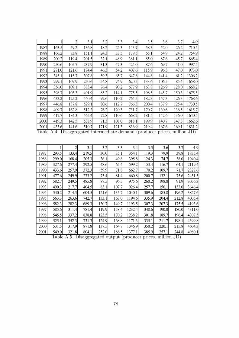
1 2 3.1 3.2 3.3 3.4 3.5 3.6 3.7 4-91987 163.5 59.2 136.8 18.2 22.3 143.7 58.3 52.0 26.2 710.51988 166.2 83.8 151.1 24.3 33.5 179.5 65.1 54.9 24.2 754.91989 200.2 119.4 201.5 32.1 48.9 381.1 85.0 87.6 45.7 865.41990 250.6 105.7 237.9 31.3 47.3 424.0 87.6 69.7 41.0 997.51991 271.0 121.6 174.4 46.3 54.2 407.6 115.9 96.3 47.0 973.01992 345.1 115.7 307.8 59.3 65.7 647.8 144.8 141.4 61.2 1306.21993 299.1 107.9 250.6 54.8 74.9 620.5 133.6 106.5 85.4 1658.01994 356.0 109.1 383.4 76.4 90.2 677.9 163.8 126.9 128.0 1668.21995 398.7 103.3 491.9 85.2 114.1 775.5 198.5 145.7 150.3 1675.51996 433.2 125.2 440.4 92.6 110.2 764.5 182.3 157.3 126.3 1768.61997 446.8 137.8 529.1 80.6 112.7 766.3 200.4 137.9 125.4 1730.51998 409.7 162.8 512.2 76.2 120.3 731.7 170.7 130.6 136.5 1615.71999 417.7 184.3 465.4 72.8 110.6 668.2 181.5 142.6 136.0 1640.52000 419.3 142.5 538.9 71.3 108.0 818.1 199.9 140.7 147.3 1662.62001 433.6 141.6 510.7 171.9 121.3 836.9 219.4 167.6 169.1 1831.2Table A.4. Disaggregated intermediate demand (producer prices, million JD)

1 2 3.1 3.2 3.3 3.4 3.5 3.6 3.7 4-91987 293.5 133.4 219.5 30.0 35.1 354.1 119.3 79.9 39.8 1835.41988 299.0 168.4 205.3 36.1 49.8 395.8 124.3 74.7 38.0 1940.41989 327.6 277.4 292.5 48.6 65.4 599.2 153.4 116.7 64.1 2119.41990 433.6 257.9 372.3 59.9 71.8 662.7 170.2 109.7 71.7 2327.61991 477.6 249.9 273.2 75.4 81.4 660.8 200.7 132.1 75.6 2451.51992 582.7 249.5 485.8 87.5 96.5 975.6 260.2 198.8 91.9 3056.31993 490.3 217.7 404.5 83.1 107.7 926.4 257.7 156.1 133.0 3646.41994 540.2 214.3 604.5 121.6 135.7 1040.1 309.6 185.8 196.2 3827.61995 563.3 263.6 742.7 133.1 163.0 1194.6 335.9 204.4 212.8 4005.41996 582.3 282.3 689.3 130.7 149.7 1193.5 307.3 207.3 175.5 4193.61997 585.6 311.4 781.4 119.9 158.4 1232.4 348.6 190.0 180.0 4311.01998 545.5 337.2 838.8 123.5 170.2 1238.2 301.8 189.7 196.4 4307.51999 525.1 352.3 731.3 124.9 168.8 1171.3 335.1 211.7 198.1 4399.82000 531.5 317.9 871.8 137.5 164.7 1346.9 350.2 220.1 215.8 4604.32001 549.0 321.8 804.1 252.0 186.5 1377.1 385.9 257.1 244.8 4980.1

Table A.5. Disaggregated output (producer prices, million JD)

78

1 2 3.1 3.2 3.3 3.4 3.5 3.6 3.7 4-91987 381.6 256.2 303.7 81.8 72.9 350.6 151.2 187.3 331.4 1580.51988 406.0 289.9 294.6 92.1 91.5 342.4 160.8 177.0 396.1 1668.31989 447.3 403.9 384.1 124.9 109.7 516.1 193.3 228.0 427.1 1838.51990 684.2 474.6 588.7 152.3 149.6 577.1 214.6 250.3 503.7 2051.01991 731.8 451.0 469.8 188.0 170.7 584.3 254.0 279.4 479.2 2128.71992 840.0 469.2 690.6 238.7 199.5 955.4 330.4 428.7 811.7 2492.61993 746.4 496.3 594.5 231.2 213.8 898.7 326.2 436.9 991.2 2817.01994 786.1 436.7 792.3 250.6 227.6 920.6 446.7 413.7 825.9 3023.71995 830.3 527.2 827.9 239.5 282.7 1033.8 473.8 497.5 867.1 3112.41996 1066.8 544.8 866.4 235.8 257.9 984.5 467.7 498.2 1037.4 2929.61997 882.5 580.3 965.4 222.0 244.9 1081.7 486.7 469.8 1050.3 3026.91998 862.5 472.4 1008.6 241.7 244.9 1103.0 436.7 420.6 1031.7 3183.81999 823.0 589.4 895.9 225.0 226.4 995.4 447.8 405.4 972.8 3251.12000 892.0 796.6 1032.6 252.6 262.0 1162.6 491.8 435.5 1267.7 3226.12001 876.2 771.2 974.7 350.0 296.2 1227.0 536.5 510.3 1225.1 3544.2

Table A.6. Supply (million JD)

2 3.1 3.2 3.3 3.4 3.5 3.6 3.7 4-91990 115 1608 1639 2448 64 1437 1832 120 55021991 119 1642 1694 2511 70 1465 1897 122 209771992 125 2062 2092 3094 111 1817 2288 117 591601993 125 2199 2109 3124 116 1846 2341 120 632171994 129 1784 1831 3292 187 2149 2825 290 676581995 131 1945 2082 3704 207 2232 3163 317 717101996 143 2002 2125 3830 221 2254 3210 330 744551997 145 2120 2206 3925 245 2345 3295 330 775631998 153 2226 2316 4084 261 2353 3383 313 9603

Table A.7. Number of firms.

a(4-9, 3.5)

0.00

0.05

0.10

0.15

0.20

0.25

0.30

1987

o19

87r

1998

1989

1990

1991

1992

1993

1994

1995

1996

1997

1998

1999

2000

2001

Figure A.1. Coefficient a(4-9,3.5)

79

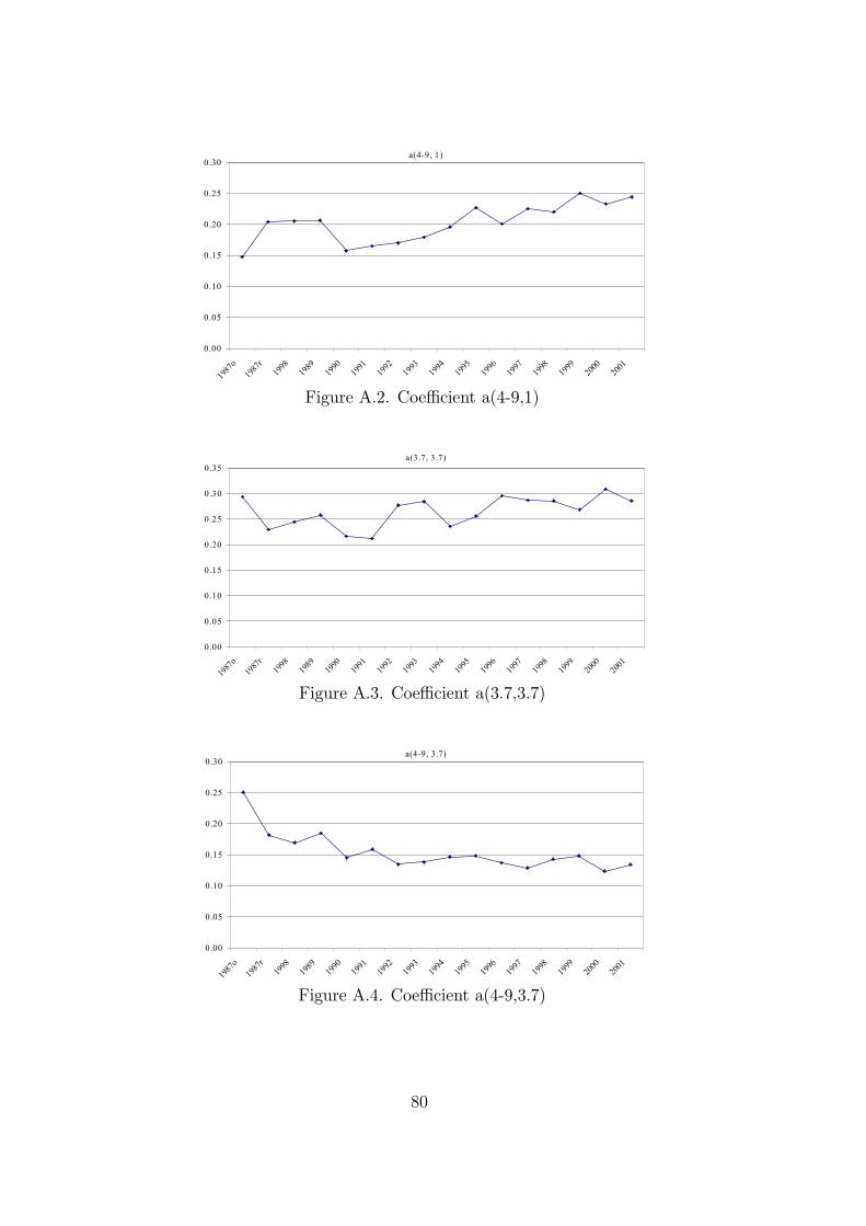
a(4-9, 1)

0.00

0.05

0.10

0.15

0.20

0.25

0.30

1987

o19

87r

1998

1989

1990

1991

1992

1993

1994

1995

1996

1997

1998

1999

2000

2001

Figure A.2. Coefficient a(4-9,1)

a(3.7, 3.7)

0.00

0.05

0.10

0.15

0.20

0.25

0.30

0.35

1987

o19

87r

1998

1989

1990

1991

1992

1993

1994

1995

1996

1997

1998

1999

2000

2001

Figure A.3. Coefficient a(3.7,3.7)

a(4-9, 3.7)

0.00

0.05

0.10

0.15

0.20

0.25

0.30

1987

o19

87r

1998

1989

1990

1991

1992

1993

1994

1995

1996

1997

1998

1999

2000

2001

Figure A.4. Coefficient a(4-9,3.7)

80

a(4-9, 3.2)

0.00

0.05

0.10

0.15

0.20

0.25

0.30

1987

o19

87r

1998

1989

1990

1991

1992

1993

1994

1995

1996

1997

1998

1999

2000

2001

Figure A.5. Coefficient a(4-9,3.2)

a(3.5, 3.5)

0.00

0.02

0.04

0.06

0.08

0.10

0.12

1987

o19

87r

1998

1989

1990

1991

1992

1993

1994

1995

1996

1997

1998

1999

2000

2001

Figure A.6. Coefficient a(3.5,3.5)

a(3.2, 3.2)

0.00

0.10

0.20

0.30

0.40

0.50

0.60

1987

o19

87r

1998

1989

1990

1991

1992

1993

1994

1995

1996

1997

1998

1999

2000

2001

Figure A.7. Coefficient a(3.2,3.2)

81

a(4-9, 4-9)

0,00

0,05

0,10

0,15

0,20

0,25

1987

o19

87r

1998

1989

1990

1991

1992

1993

1994

1995

1996

1997

1998

1999

2000

2001

Figure A.8. Coefficient a(4-9,4-9).

a(3.1, 1)

0,00

0,05

0,10

0,15

0,20

0,25

0,30

0,35

0,40

1987

o19

87r

1998

1989

1990

1991

1992

1993

1994

1995

1996

1997

1998

1999

2000

2001

Figure A.9. Coefficient a(3.1,1)

82

6.2 Appendix 2. The Standard Trade Model

2.A. List of equations

(time index dropped for simplicity)

Capital accumulation equation

K = I − δK

Disposable income

Y D =¡1− tY ¢ £wL+ ¡1− tK¢ rK + TR+ erFREM¤

Euler equation

C

C=

¡1− tY ¢ ¡1− tK¢ r

P I− ρ− δ

Composite private consumption

C = ΩCNYi=1

cθCii ;Ω

C > 0; 0 < θCi < 1

PCC =

NXi=1

PXi ci

ci

cj=

θCi PXj

θCj PXi

; i, j = 1, 2, ..,N

Consumption price index

PC =1

ΩC

NYi=1

µPXi

θCi

¶θCj

; N = 10

Private consumption demand functions

ci = θCiPCC

PXi

83

Composite government consumption

G = ΩGNYi=1

gθGii ; Ω

G > 0; 0 < θGi < 1

PGG =

NXi=1

PXi gi

gi

gj=

θGi PXj

θGj PXi

; i, j = 1, 2, .., N

Government consumption price index

PG =1

ΩG

NYi=1

µPXi

θGi

¶θGj

; N = 10

Government consumption demand functions

gi = θGiPCG

PXi

Composite investment

I = ΩINYi=1

invθIii ; Ω

I > 0; 0 < θIi < 1

P II =

NXi=1

PXi invi

invi

invj=

θIiPXj

θIjPXi

; i, j = 1, 2, .., N

Investment price index

84

P I =1

ΩI

NYi=1

µPXi

θIi

¶θIj

; N = 10

Investment demand functions

invi = θIiP II

PXi

Leontief production function

Qi = min

½V Ai

a0,i,qj,i

aj,i, ....

¾; i, j = 1, 2, ..,N

Value-added production function

V Ai = Ai

"αiLD

σi−1σi

i + (1− αi)KD

σi−1σi

i

# σiσi−1

; 0 < αi < 1; σi > 0; σi 6= 1

P V Ai V Ai = wLDi + rKDi

KDi

LDi=

∙w

r

(1− αi)

αi

¸σiLabour demand function

LDi = (Ai)(σi−1) V Ai

µαiP

V Ai

w

¶σi

Capital demand

KDi = (Ai)(σi−1) V Ai

∙(1− αi)P

V Ai

r

¸σiValue-added price

P V Ai =1

Ai

£w(1−σi) (αi)

σi + r(1−σi) (1− αi)σi¤ 11−σi

85

CES Armington function

The equations below have been used in the calibration procedure in a general form;

more specifically, in the model the same equations apply to private consumption,

government consumption, investment and intermediate inputs: therefore Xi has to

be replaced by ci, gi, invi and qj,i; Mi has to replaced by cmi, gmi, invmi and qmj,i;

and cdi, gdi, invdi and qdj,i will replace Di, where the subscripts i and j indicate

the production sector; functional parameters and prices are the same for all specific

forms.

Xi = Φi

∙εi (Mi)

γi−1γi + (1− εi) (Di)

γi−1γi

¸ γiγi−1

Φi > 0; 0 < εi < 1; γi > 0; γi 6= 1; i = 1, 2, ..., 10

PXi Xi = PMi Mi +

¡1 + vatDi

¢PDi Di

Di

Mi=

∙(1− εi)P

MFi

εi (1 + vatDi )P

Di

¸γiImports demand function

Mi = (Φi)(γi−1)Xi

µεiP

Xi

PMi

¶γi

Domestic goods demand function

Di = (Φi)(γi−1)Xi

∙(1− εi)P

Xi

(1 + vatDi )PDi

¸γiComposite CES Armington price

PXi =1

Φi

n¡PMi

¢(1−γi) (εi)γi + £¡1 + vatDi ¢PDi ¤(1−γi) (1− εi)γio 11−γi

Cobb-Douglas total imports

The equations for total imports have been used in the calibration procedure in the

general form described below; in the model, the same equations apply to private con-

sumption, government consumption, investment and intermediate inputs: therefore

86

Mi has to replaced by cmi, gmi, invmi and qmj,i; and Mji will be replaced by cm

ji ,

gmji , invm

ji and qm

ji,k, where i and k are production sector indeces and j is index

indicating the foreign region; functional parameters and prices are the same for all

specific forms.

Mi = ΦMi¡MEUi

¢εEUi ¡MRWi

¢εRWiΦMi > 0; 0 < εEUi , εRWi < 1; εEUi + εRWi = 1; i = 1, 2, ..,N

PMi Mi = PMEUi MEU

i + PMRWi MRW

i

MEUi

MRWi

=εEUi PMRW

i

εRWi PMEUi

Regional imports demand functions

Mji = ε

ji

PMi Mi

PMji

; i = 1, 2, .., 10; j = EU,RW

Import composite price

PMi =1

ΦMi

µPMEU

i

εEUi

¶εEUiµPMRW

i

εRWi

¶εRWi

Import prices

PMji = erPWMi

¡1 + tm

ji

¢ ¡1 + vatMi

¢; j = EU,RW

CET function

Qi = χi

∙λi (Ei)

1+ΨiΨi + (1− λi) (Di)

1+ΨiΨi

¸ Ψi1+Ψi

χi > 0; 0 < λi < 1; Ψi > 0; i = 1, 2, ..., N

PQi Qi = P

Ei Ei + P

Di Di

87

Di

Ei=

∙λiP

Di

(1− λi)PEi

¸ΨiExport supply function

Ei =Qi

(χi)(1+Ψi)

³PQi

´Ψi µPEiλi¶Ψi

Domestic good supply function

Di =Qi

(χi)(1+Ψi)

³PQi

´Ψi µ PDi1− λi

¶Ψi

Composite output price

PQi =

1

χi

"¡PEi¢(1+Ψi)

(λi)Ψi

+

¡PDi¢(1+Ψi)

(1− λi)Ψi

# 11+Ψi

CET composite exports

Ei = χEi

"λEUi

¡EEUi

¢1+ΨEiΨEi + λRWi

¡ERWi

¢1+ΨEiΨEi

# ΨEi1+ΨEi

χEi > 0; 0 < λEUi ,λRWi < 1; λEUi + λRWi = 1; ΨEi > 0; i = 1, 2, , .., N

PEi Ei = PEEUi EEUi + PERWi ERWi

EEUiERWi

=

µλRWi PEEUi

λEUi PERWi

¶ΨEi

Exports supply functions

Eji =

Ei

(PEi )ΨEi (χEi )

(1+ΨEi )

ÃPE

ji

λji

!ΨE

; i = 1, 2, , .., N ; j = EU,RW

88

Export composite price

PEi =1

χEi

"¡PEEUi

¢1+ΨEi(χEi )

ΨEi+

¡PERWi

¢1+ΨEi(χDi )

ΨEi

# 11+ΨEi

Export prices

PEji = erPWEi; j = EU,RW

Domestic goods VAT revenue

V ATD =

NXi=1

vatDi PDi Di

Imported goods VAT revenue

V ATM =

NXi=1

Xj=EU,RW

vatMi¡1 + tm

ji

¢erPWM

i Mji

Imports tariffs revenue

TM =

NXi=1

Xj=EU,RW

tmjierPW

Mi M

ji

Capital rent tax revenue

TK = tKrK

Income tax revenue

TY = ti£wL+

¡1− tK¢ rK + TR + erFREM

¤Government budget

V ATD + V ATM + TY + TK + TM + erFRG = TR+G

89

Labour market equilibrium

L =

NXi=1

LDi

Capital goods market equilibrium

K =

NXi=1

KDi

Domestic goods markets equilibrium

Xi =

NXj=1

qi,j + ci + invi + gi

External equilibrium

NXi=1

PWMi Mi =

NXi=1

PWEi Ei + FREM + FGR

2.B. Glossary

N : number of production sectors (N = 10)

er: exchange rate (numeraire)

L: labour supply

K: capital supply

C: private consumption

PC : private consumption price index

Y D: personal disposable income

TR: government transfers to households

FREM : foreign remittances to households

tY : income tax rate

tK: tax on capital income

ρ: household’s discount rate

δ: deprecation rate of capital

90

PXi : composite price of good i

ci: household’s consumption of good i

ΩC : shift parameter in the Cobb-Douglas private consumption function

θCi : good i’s share parameter in the Cobb-Douglas private consumption function

I: aggregate investment

P I : price index of aggregate investment

invi: sector i’s investment demand

ΩI : shift parameter in the Cobb-Douglas investment function

θIi : good i’s share parameter in the Cobb-Douglas investment function

G: aggregate government consumption

PG: price index of aggregate government consumption

gi: government consumption of good i

ΩG: shift parameter in the Cobb-Douglas government consumption function

θGi : good i’s share parameter in the Cobb-Douglas government consumption func-

tion

V Ai: sector i’s value-added production

P V Ai : sector i’s value-added price

LDi: sector i’s demand for labour

KDi: sector i’s demand for capital

Ai: shift parameter of the value-added production function in sector i

σi: elasticity of substitution between primary inputs in sector i

αi: share parameter of labour used in the production of good i

w: nominal wage rate

r: nominal return to capital

Qi: total output of sector i

PQi : composite output price of sector i

qj,i: intermediate input produced by sector j used in the production of sector i

a0,i: fixed coefficient of value-added output for sector i’s production

aj,i: fixed coefficient of intermediate input j in the production of good i

Xi: total domestic absorption of sector i

Mi: total imports of sector i

cmi: private consumption demand for import good produced by sector i

gmi: government consumption demand for import good produced by sector i

invmi: investment demand for import good produced by sector i

91

qmj,i: imported intermediate input produced by sector j used in the production

of sector i

Di: total domestic production of sector i

cdi: private consumption demand for domestic good produced by sector i

gdi: government consumption demand for domestic good produced by sector i

invdi: investment demand for domestic good produced by sector i

qdj,i: intermediate input produced domestically by sector j used in the production

of sector i

Φi: shift parameter in the CES Armington function of sector i

εi: imports share parameter in the CES Armington function of sector i

γi: sector i’s elasticity of substitution between imports and domestically-produced

output

PXi : composite price of domestic absorption of sector i

PMi : import price of sector i

PDi : price of sector i’s domestically-produced good

vatDi : VAT rate on sector i’s domestically-produced good

Mji : imports of sector i from region j

cmji : private consumption of good i imported from region j

gmji : government consumption of good i imported from region j

invmji : investment demand for good i imported from region j

qmji,k: intermediate input consumption of good i used in the production of sector

k and imported from region j

PMji : sector i’s price of imports from region j

ΦMi : shift parameter in the imports CES function of sector i

εji : region j’s share parameter in the imports CES function of sector i

tmji : import tax rate applying to sector i’s imports from region j

vatMi : VAT rate on sector i’s imported goods

PWMi : sector i’s world price of imports

Ei: total exports of sector i

PEi : export price of sector i

χi: shift parameter in the CET function of sector i

λi: export share parameter of sector i

Ψi: elasticity of transformation between exports and domestically-sold output of

sector i

92

Eji : total exports of sector i to region j

χEi : shift parameter in the CET exports function of sector i

λji : share parameter of exports to region j in sector i

ΨEi : elasticity of transformation between exports to different regions of sector i

PEji : price of exports to region j of sector i

PWEi : world price of exports of sector i

V ATD: domestic goods VAT revenue

V ATM : imported goods VAT revenue

TM : aggregate import tariffs revenue

TK: capital tax revenue

TY : income tax revenue

FRG: foreign grants to the government

93

6.3 Appendix 3. The Poverty Model

3.A. List of equations

(time index dropped for simplicity)

Capital accumulation equation

Ki = SAVi − δKi = −Y Di − PCCiPI

− δKi, i = 1, 2, .., H

Disposable income

Y Di = (1− τ i)(wiLi + rKi + Tri + erFTi)

Euler equation

Ci

Ci=(1− τ i) r

P I− ρi − δ

Composite private consumption

Ci = ΩCi

NYj=1

cθCi,ji,j ; Ω

Ci > 0; 0 < θCi,j < 1; i = 1, 2, .., H; j = 1, 2, .., N

PCi Ci =

NXj=1

PXj ci,j

ch,i

ch,j=

θCh,ipcj

θCh,jpci; i, j = 1, 2, .., N ; h = 1, 2, , .., H

Consumption prices

PCi =1

ΩCi

NYj=1

ÃPXj

θCi,j

!θCij

Private consumption demand functions

ci,j = θCi,jPCi Ci

PXj

94

Composite government consumption

G = ΩGNYj=1

gθGjj ; Ω

G > 0; 0 < θGj < 1; j = 1, 2, ..., N

PGG =

NXi=j

PXj gj

gi

gj=

θGi PXj

θGj PXi

; i, j = 1, 2, .., N

Government consumption price index

PG =1

ΩG

NYj=1

ÃPXj

θGj

!θGj

Government consumption demand functions

gj = θGjPCG

PXj

Composite investment

I = ΩINYj=1

invθIjj ; Ω

I > 0; 0 < θIj < 1; j = 1, 2, .., N

P II =

NXj=1

PXj invj

invi

invj=

θIiPXj

θIjPXi

; i, j = 1, 2, .., N

Investment price index

95

P I =1

ΩI

NYj=1

ÃPXj

θIj

!θIj

Investment demand functions

invj = θIjP II

PXj

Leontief production function

Qj = min

½V Aj

a0,j,qi,j

ai,j, ....

¾Value-added production function

V Aj = Aj

"HPi=1

αi,jLD

σj−1σj

i,j +

µ1−

HPi=1

αi,j

¶KD

σj−1σj

j

# σjσj−1

i = 1, 2, ..,H; j = 1, 2, ..,N

P V Aj V Aj =

HXi=1

wiLDi,j + rKDj

Labour demand functions

Li,j = (Aj)(σj−1) V Aj

Ãαi,jP

V Aj

wi

!σj

Capital demand

Kj = (Aj)(σj−1) V Aj

⎡⎢⎢⎣µ1−

NPi=1

αi,j

¶P V Aj

r

⎤⎥⎥⎦σj

Value-added price

96

P V Aj =1

Aj

"NXi=1

(wi)(1−σj) (αi,j)

σj + r(1−σj)Ã1−

NXi=1

αij

!σj# 11−σj

CES Armington function

The equations below have been used in the calibration procedure in a general form;

more specifically, in the model the same equations apply to private consumption,

government consumption, investment and intermediate inputs: therefore Xi has to

be replaced by ch,i, gi, invi and qj,i; Mi has to replaced by cmi, gmi, invmi and qmj,i;

and cdi, gdi, invdi and qdj,i will replaceDi, where the subscript h stands for household

and the subscripts i and j indicate the production sector; functional parameters and

prices are the same for all specific forms.

Xi = Φi

∙εi (Mi)

γi−1γi + (1− εi) (Di)

γi−1γi

¸ γiγi−1

Φi > 0; 0 < εi < 1; γi > 0, γi 6= 1; i = 1, 2, ..., N

PXi Xi = PMi Mi +

¡1 + vatDi

¢PDi Di

Di

Mi=

∙(1− εi)P

MFi

εi (1 + vatDi )P

Di

¸γiImports demand function

Mi = (Φi)(γi−1)Xi

µεiP

Xi

PMi

¶γi

Domestic goods demand function

Di = (Φi)(γi−1)Xi

∙(1− εi)P

Xi

(1 + vatDi )PDi

¸γiComposite CES Armington price

PXi =1

Φi

n¡PMi

¢(1−γi) (εi)γi + £¡1 + vatDi ¢PDi ¤(1−γi) (1− εi)γio 1

1−γi

97

Cobb-Douglas total imports

The equations for total imports have been used in the calibration procedure in

the general form described below; in the model, the same equations apply to private

consumption, government consumption, investment and intermediate inputs: there-

fore cmh,i, gmi, invmi and qmi,k replace Mi; and cmjh,i, gm

ji , invm

ji and qm

ji,k, where

the subscripts i and k are production sector indeces, the superscript j indicates the

foreign region, and the index h stands for household.

Mi = ΦMi¡MEUi

¢εEUi ¡MRWi

¢εRWiΦMi > 0; 0 < εEUi , εRWi < 1; εEUi + εRWi = 1; i = 1, 2, ..,N

PMi Mi = PMEUi MEU

i + PMRWi MRW

i

MEUi

MRWi

=εEUi PMRW

i

εRWi PMEUi

Regional imports demand functions

Mji = ε

ji

PMi Mi

PMji

; i = 1, 2, .., N ; j = EU,RW

Import composite price

PMi =1

ΦMi

µPMEU

i

εEUi

¶εEUiµPMRW

i

εRWi

¶εRWi

Import prices

PMji = erPWMi

¡1 + tm

ji

¢ ¡1 + vatMi

¢; j = EU,RW

CET function

Qi = χi

hλi (Ei)

1+ΨiΨi + (1− λi) (Di)

1+ΨiΨi

i Ψi1+Ψi

χi > 0, 0 < λi < 1, Ψi > 0, i = 1, 2, ..., N

98

PQi Qi = P

Ei Ei + P

Di Di

Di

Ei=

∙λiP

Di

(1− λi)PEi

¸ΨiExport supply function

Ei =Qi

(χi)(1+Ψi)

³PQi

´Ψi µPEiλi¶Ψi

Domestic good supply function

Di =Qi

(χi)(1+Ψi)

³PQi

´Ψi µ PDi1− λi

¶Ψi

Composite output price

PQi =

1

χi

"¡PEi¢(1+Ψi)

(λi)Ψi

+

¡PDi¢(1+Ψi)

(1− λi)Ψi

# 11+Ψi

CET composite exports

Ei = χEi

"λEUi

¡EEUi

¢ 1+ΨEiΨEi + λRWi

¡ERWi

¢ 1+ΨEiΨEi

# ΨEi1+ΨE

i

χEi > 0; 0 < λEUi ,λRWi < 1; λEUi + λRWi = 1; ΨEi > 0; i = 1, 2, , .., N

PEi Ei = PEEUi EEUi + PERWi ERWi

EEUiERWi

=

µλRWi PEEUi

λEUi PERWi

¶ΨEi

Exports supply functions

99

Eji =

Ei

(PEi )ΨEi (χEi )

(1+ΨEi )

µPEi

λji

¶ΨE

; i = 1, 2, , .., N ; j = EU,RW

Export composite price

PEi =1

χEi

"¡PEi¢1+ΨEi

(χEi )ΨEi

+

¡PDi¢1+ΨEi

(χDi )ΨEi

# 1

1+ΨEi

Export prices

PEji = erPW

Ei ; j = EU,RW

Domestic goods VAT revenue

V ATD =

NXi=1

vatDi PDi Di

Imported goods VAT revenue

V ATM =

NXi=1

Xj=EU,RW

vatMi¡1 + tm

ji

¢erPWM

i Mji

Import duties revenue

TM =

NXi=1

Xj=EU,RW

tmjiPW

Mi M

ji

Income tax revenue

TY =

HXi=1

τ i(wiLi + rKi + Tri + erFTi)

Aggregate government transfers to households

TR =

HXi=1

Tri

Government transfer to each household class

100

Tri = πiTR; 0 < πi < 1;

HXi=1

πi = 1

Government budget

V ATD + V ATM + TY + TM + erFRG = TR+G

Labour market equilibrium conditions

Li =

NXj=1

LDi,j; for each i = 1, .., H

Capital goods market equilibrium

HXi=1

Ki =

NXj=1

KDj

Domestic goods markets equilibrium

Xj =

NXi=1

qi,j +

HXh=1

ch,j + invj + gj

External equilibrium

NXj=1

PWMj Mj =

NXj=1

PWEj Ej +

HXi=1

FTi + FGR

3.B. Glossary

H: number of households (H = 6)

N : number of production sectors (N = 9)

er: exchange rate (numeraire)

SAVi: saving of household i

Y Di: disposable income of household i

101

Tri: government tranfer to household i

FTi: foreign remittances to household i

Ci: total consumption of household i

PCi : consumption price (index) of household i

τ i: income tax rate applying to household i

ρi: household i’s discount rate

ΩCi : shift parameter in the private consumption Cobb-Douglas consumption func-

tion of household i

ci,j: household i’s consumption of good j

PXj : composite price of good j

θCi,j : share parameter in the private consumption Cobb-Douglas function of house-

hold i for good j

I: aggregate investment

P I : price index of aggregate investment

invi: sector i’s investment demand

ΩI : shift parameter in the Cobb-Douglas investment function

θIi : good i’s share parameter in the Cobb-Douglas investment function

G: aggregate government consumption

PG: price index of aggregate government consumption

gi: government consumption of good i

ΩG: shift parameter in the Cobb-Douglas government consumption function

θGi : good i’s share parameter in the Cobb-Douglas government consumption func-

tion

δ: deprecation rate of capital

Li,j : sector j’s demand for labour of type i

Kj: sector j’s demand for capital

Aj : shift parameter of the value-added production function in sector j

σj : elasticity of substitution between primary inputs in sector j

αi,j: share parameter of labour of type i used in sector j

V Aj : sector j’s value-added production

P V Aj : sector j’s value-added price

wi: nominal wage rate of labour of type i

r: nominal return to capital

Xi: domestic absorption of sector i

102

Mi: total imports of sector i

cmi: private consumption demand for import good produced by sector i

gmi: government consumption demand for import good produced by sector i

invmi: investment demand for import good produced by sector i

qmj,i: imported intermediate input produced by sector j used in the production

of sector i

Di: domestic production of sector i

cdi: private consumption demand for domestic good produced by sector i

gdi: government consumption demand for domestic good produced by sector i

invdi: investment demand for domestic good produced by sector i

qdj,i: intermediate input produced domestically by sector j used in the production

of sector i

Φi: shift parameter in the CES Armington function of sector i

εi: imports share parameter in the CES Armington function of sector i

γi: sector i’s elasticity of substitution between imports and domestically-produced

output

PXi : composite price of domestic absorption of sector i

PMi : import price of sector i

PDi : price of sector i’s domestically-produced good

vatDi : VAT rate on sector i’s domestically-produced good

Mji : imports of sector i from region j

cmji : private consumption of good i imported from region j

gmji : government consumption of good i imported from region j

invmji : investment demand for good i imported from region j

qmji,k: intermediate input consumption of good i used in the production of sector

k and imported from region j

PMji : sector i’s price of imports from region j

ΦMi : shift parameter in the imports CES function of sector i

εji : region j’s share parameter in the imports CES function of sector i

tmji : import tax rate applying to sector i’s imports from region j

vatMi : VAT rate on sector i’s imported goods

PWMi : sector i’s world price of imports

Qi: total output of sector i

PQi : composite output price of sector i

103

Ei: total exports of sector i

PEi : export price of sector i

χi: shift parameter in the CET function of sector i

λi: export share parameter of sector i

Ψi: elasticity of transformation between exports and domestically-sold output of

sector i

Eji : exports of sector i to region j

χEi : shift parameter in the CET exports function of sector i

λji : share parameter of exports to region j in sector i

ΨEi : elasticity of transformation between exports to different regions of sector i

PEji : price of exports to region j of sector i

PWEi : world price of exports of sector i

V ATD: domestic goods VAT revenue

V ATM : imported goods VAT revenue

TM : aggregate import tariffs revenue

TY : income tax revenue

TR: aggregate government transfers to households

FRG: foreign grants to the government

104

References

[1] Abed, G.T., 1998, Trade Liberalization and Tax Reform in the Southern Mediter-

ranean Countries, IMF Working Paper 49.

[2] Aisbett, E., 2005, Why are the Critics so Convinced that Globalization is Bad

for the Poor?, NBER Working Paper No. 11066.

[3] Armington, P.S., 1969, A Theory of Demand for Products Distinguished by Place

of Production, IMF Staff Papers 16, 159-176.

[4] Bacharach, M., 1970, Biproportional Matrices and Input-Output Change, Cam-

bridge University Press.

[5] Baldwin, R., 1993, On the Measurement of Dynamic Effects of Integration, Em-

pirica, 20, 129-145.

[6] Bandara, J.S., 1991, Computable General Equilibrium Models for Development

Policy Analysis in LDCs, Journal of Economic Surveys 5(1), 3-69.

[7] Bautista, R.M, Lofgren, H. and Thomas, M., 1998, Does Trade Liberalization

Enhance Income, Growth and Equity in Zimbabwe? The Role of Complementary

Policies, TMD Discussion Paper No. 32, International Food Policy Research

Institute.

[8] Blanchard, O.J. and Fischer, S., 1998, Lectures on Macroeconomics, MIT Press.

[9] Bourguignon, F., Branson, W.H. and de Melo, J., 1992, Adjustment and In-

come Distribution. A micro-macro model for counterfactual analysis, Journal of

Development Economics 38, 17-39.

[10] Bulmer-Thomas, V., 1982, ”Input-Output Analysis in Developing Countries”,

John Wiley and Sons.

[11] Casella, F. and Ventura, J., 2000, A Representative Consumer Theory of Distri-

bution, American Economic Review 90, 909-926

[12] Cass, D., 1995, Optimum Growth in an Aggregate Model of Capital Accumula-

tion, Review of Economic Studies 32, 233-240.

105

[13] Chatterjee, S., 1994, Transitional Dynamics and the Distribution of Wealth in a

Neoclassical Growth Model, Journal of Public Economics 54, 97-119.

[14] Cockburn, J., 2001, Trade Liberalisation and Poverty in Nepal: A Computable

General Equilibrium Micro Simulation Analysis, Discussion paper 01-18, Centre

de Recherche en Economie et Finance Appliquees, Universite Laval.

[15] Decaluwe, B., Patry, A., Savard, L. and Thorbecke, E., 1999, Poverty Anal-

ysis Within a General Equilibrium Framework, Working Paper 9909, CREFA,

University of Laval.

[16] de Melo, J., 1988, Computable General Equilibrium Models for Trade Policy

Analysis in Developing Countries: A Survey, Journal of Policy Modeling 10(4),

469-503.

[17] Devarajan, S., Lewis, J.D. and Robinson, S., 1990, Policy Lessons from Trade-

Focused, Two-Sector Models, Journal of Policy Modeling 12(4), 625-657.

[18] Devarajan, S., Go, D.S., Lewis, J.D., Robinson, S. and Sinko, P., 1997, Sim-

ple General Equilibrium Modeling, in Francois, J.F. and Reinert, K.A. (eds.),

Applied Methods for Trade Policy Analysis, Cambridge University Press.

[19] Devarajan, S. and Go, D.S., 1998, The Simplest Dynamic General-equilibrium

Model of an Open Economy, Journal of Policy Modeling 20(6), 677-714

[20] Devarajan, S., Go, D.S. and Li, H., 1999, Quantifying the fiscal effects of trade

reform: A general equilibrium model estimated for 60 countries, World Bank

Policy Research Working Paper 2162.

[21] Feraboli, O., Lucke, B. and Gaitan Soto, B., 2003, Trade Liberalisation and

the Euro-Med Partnership: A Dynamic Model for Jordan, Discussion Paper,

University of Hamburg.

[22] Francois, J.F., McDonald, B.J. and Nordstrom, H., 1997, Capital Accumulation

in Applied Trade Models, in Francois, J.F. and Reinert, K.A. (eds.), Applied

Methods for Trade Policy Analysis, Cambridge University Press.

[23] Gini, C., 1912, Variabilita e mutabilita. Reprinted in Memorie di metodologia

statistica, Ed. Pizzetti E. and Salvemini, T., Libreria Eredi Virgilio Veschi, 1955.

106

[24] Harrison, G.W., Rutherford, T.F. and Tarr, D.G., 1997, Quantifying the

Uruguay Round, The Economic Journal 107, 1405-1430.

[25] Harrison, G.W., Rutherford, T.F., Tarr, D.G. and Gurgel, A., 2003, Regional,

Multilateral and Unilateral Trade Policies of MERCOSUR for Growth and

Poverty Reduction in Brazil, World Bank Policy Research Working Paper No.

3051.

[26] Hertel, T.W., Preckel, P.V., Cranfield, J.A.L. and Ivanic, M., 2002, Poverty Im-

pacts of Multilateral Trade Liberalization, GTAP Working Paper, Center for

Global Trade Analysis, Department of Agricultural Economics, Purdue Univer-

sity.

[27] Hirsch, M.W., Pugh, C.C. and Shub, M., 1977, Invariant Manifolds, Springer-

Verlag.

[28] Hoekman, B. and Djankov, S., 1997, Effective Protection and Investment Incen-

tives in Egypt and Jordan During the Transition to Free Trade With Europe,

World Development 25(2), 281-291.

[29] Hoekman, B. and Konan, D.E., 1999, Deep Integration, Nondiscrimination, and

Euro-Mediterranean Free Trade, Policy Research Working Paper Series No. 2130,

World Bank.

[30] Hosoe, N., 2001, A General equilibrium analysis of Jordan’s trade liberalization,

Journal of Policy Modeling 23, 595-600.

[31] Ianchovichina, E., Nicita, A. and Soloaga, I., 2001, Trade Reform and Household

Welfare: The Case of Mexico, Policy Research Working Paper No. 2667, The

World Bank Development Research Trade Group.

[32] IMF, 2005, Public Information Notice No. 06/56 of May 23, 2005.

[33] Koopmans, T.C., 1965, On the Concept of Optimal Growth Theory, in The

Econometric Approach to Development Planning, North Holland.

[34] Leontief, W., 1966, ”Input-Output Economics”, Oxford University Press.

107

[35] Lofgren, H., El-Said, M. and Robinson, S., 1999, Trade Liberalization and Com-

plementary Domestic Policies: A Rural-Urban General Equilibrium Analysis of

Morocco, TMD Discussion Paper No. 41, International Food Policy Research

Institute.

[36] Lofgren, H., 2001, Less Poverty in Egypt? Explorations od Alternative Pasts

with Lessons for the Future, TMD Discussion Paper No. 72, International Food

Policy Research Institute.

[37] Lucke, B., 2001, Fiscal Impact of Trade liberalisation: The Case of Syria,

FEMISE Reserach Programme Paper.

[38] Lucke, D., 2001, Fiscal Impact of Trade Liberalization: The Case of Jordan,

FEMISE Research Programme Final Report.

[39] Martin, W., 2000, Assessing the Implications for Lebanon of Free Trade with the

European Union, World Bank, Development Research Group.

[40] Oxfam International, 2003, The Euro-Mediterranean Agreements. Partnership

or Penury?, Oxfam Briefing Paper 57.

[41] Oxfam International, 2005, Euro-Med: ensuring a fair deal, Oxfam Briefing Note

26 November.

[42] Pereira, A.M., and Shoven, J.B., 1988, Survey of Dynamic Computational Gen-

eral Equilibrium Models for Tax Policy Evaluation, Journal of Policy Modeling

10(3), 401-436.

[43] Ramsey, F., 1928, A Mathematical Theory of Saving, Economic Journal 38, 543-

559.

[44] Reimer, J.J., 2002, Estimating the Poverty Impacts of Trade Liberalization, Pol-

icy Research Working Paper Series 2790, World Bank.

[45] Shoven, J.B., 1983, Applied General-Equilibrium Tax Modeling, IMF Staff Pa-

pers 30(2), 394-420.

[46] Shoven, J.B., and Whalley, J., 1984, Applied General-Equilibrium Models of

Taxation and International Trade: An Introduction and Survey, Journal of Eco-

nomic Literature XXII, 1007-1051.

108

[47] Shoven, J.B., and Whalley, J., 1992, Applying general equilibrium, Cambridge

University Press.

[48] Theil, H., 1967, Economic and Information Theory, North Holland.

[49] Trimborn, T., 2006, A Numerical Procedure for Simulating Models of Endoge-

nous Growth, Discussion Paper, University of Hamburg.

[50] Trimborn, T., Koch, K. and Steger, T.M., 2004, Multi-Dimensional Transitional

Dynamics: A Simple Numerical Procedure, ETH Working Paper 04/35.

[51] Tu, P.N., 1994, Dynamical Systems, An Introduction with Applications in Eco-

nomics and Biology, Springer-Verlag.

[52] Winters, L.A., 1999, Trade Poverty: Is There a Connection?, in Trade, Income

Disparity and Poverty, WTO Special Study.

[53] Winters, L.A., McCulloch, N. and McKay, A., 2004, Trade Liberalisation and

Poverty: The Evidence So Far, Journal of Economic Literature XLII, 72-115.

109