a dsge model for a soe with systematic interest and ... · dynare working papers series a dsge...
TRANSCRIPT

Dynare Working Papers Serieshttp://www.dynare.org/wp/
A DSGE model for a SOE with Systematic Interest andForeign Exchange policies in which policymakers exploit
the risk premium for stabilization purposes
Guillermo J. Escude
Working Paper no. 15
September 2012
142, rue du Chevaleret — 75013 Paris — Francehttp://www.cepremap.ens.fr
1
A DSGE model for a SOE with Systematic Interest and Foreign Exchangepolicies in which policymakers exploit the risk premium for stabilizationpurposes1Guillermo J. EscudéCentral Bank of ArgentinaAbstract: This paper builds a DSGE model for a SOE in which the central banksystematically intervenes both the domestic currency bond and the FX marketsusing two policy rules: a Taylor-type rule and a second rule in which the operationaltarget is the rate of nominal currency depreciation. For this, the instruments usedby the central bank (bonds and international reserves) must be included in themodel, as well as the institutional arrangements that determine the total amountof resources the central bank can use. The �corner�regimes in which only one ofthe policy rules is used are particular cases of the model. The model is calibratedand implemented in Dynare for 1) simple policy rules, 2) optimal simple policyrules, and 3) optimal policy under commitment. Numerical losses are obtained forad-hoc loss functions for di¤erent sets of central bank preferences (styles). Theresults show that the losses are systematically lower when both policy rules are usedsimultaneously, and much lower for the usual preferences (in which only in�ationand/or output stabilization matter). It is shown that this result is basically due tothe central bank�s enhanced ability, when it uses the two policy rules, to in�uencecapital �ows through the e¤ects of its actions on the endogenous risk premium inthe (risk-adjusted) interest parity equation.JEL classi�cation: E58, F41, O24Keywords: DSGE models, Small Open Economy, Exchange rate policy, Optimal
policy
1The views expressed in this paper are the author�s and do not necessarily re�ect those ofthe Central Bank of Argentina. A previous version was presented to the 7th Dynare Conferenceat the Federal Reserve Bank of Atlanta, September 9-10, 2011, under the title "Optimal (andsimultaneous) Interest and Foreign Exchange feedback policies in a DSGE model for a small openeconomy". Comments and suggestions by Horacio Aguirre to a previous version of this paper aregratefully acknowledged.

2
1. IntroductionAccording to John Williamson �the overwhelming conventional view in the pro-fession is that it is a mistake to try to manage exchange rates� (J. Williamson(2007)), although he does not subscribe this view. After having for a long timerecommended a basket, band, and crawl (BBC) regime, Williamson lately confessesto have converted to the cause of in�ation targeting, but with some signi�cant ad-ditional ingredients: �most of the time the only monetary policy objective that maymerit consideration -other than in�ation targeting- is the maintenance of a su¢ -ciently competitive exchange rate to preserve the incentive to invest�... (in tradablesectors). He also argues that �the government can expect to reduce misalignmentsby a policy of intervention. The question is how those interventions should bestructured: whether they should be ad-hoc or systematic and, if the latter, howthe system should be designed.� This paper attempts to deal with these issues ina novel way, integrating the usual �in�ation targeting�(or Taylor rule) approachwith a policy of systematic intervention in the foreign exchange market.In my view there is no justi�cation for having to choose between an in�ation
target anchor and an exchange rate target anchor. But it is by no means easyto escape this dichotomy in the absence of an accepted and adequate theoreticalframework. My hunch is that this absence is due to the pervasive preference ofmodelers (theoreticians) to �sweep under the rug�some of the Central Bank �nutsand bolts�that are necessary to achieve a more general theory. Such �nuts and bolts�as the Central Bank balance sheet (and the �nancial assets and liabilities withinit), are detailed and analyzed in any IMF Article IV mission report pertainingto developing countries. However, when it comes to modeling the macroeconomy.such aspects are simply omitted in both academic and IMF models. What makessuch an omission possible, of course, is that if we accept the dichotomy in question,an argument of system decomposability allows one to focus on the central block ofequations. However, if we do not accept the dichotomy, the need to include such�nuts and bolts�arises merely to ensure a consistent policy model.This paper, and the model on which it is based, attempts to build such a
consistent policy model. Using the model with various policy frameworks (simplepolicy rules, optimal simple policy rules, optimal policy under commitment) andimplementing a �rst order approximation using Dynare, I �nd strong evidencethat a proper systematic use by Central Banks (CBs) of small open economies(SOEs) of two policy rules, one for the nominal interest rate and another for therate of nominal depreciation, outperforms the �corner�regimes of in�ation targeting(�oating exchange rate) and an exchange rate peg. The basic di¤erence between themodel used here and the workhorse DSGE model of the profession is the inclusionof more detail in the modeling of the institutional structure that takes us closer toa formal representation of how most CBs (at least those in developing economies)implement their interest and foreign exchange policies. However, as far as I amaware no CB implements its FX policy the way that it is modeled in this paper.When FX policy is systematic, there tends to be an exchange rate-related target.And when there is an explicit in�ation targeting framework, FX policy tends tobe highly discretional. One of the conclusions of this paper is that it is perfectlypossible to articulate a consistent model which conserves the systematic interestrate policy rule that prevails in the literature (Taylor rule models) yet incorporates
3
an additional policy rule to represent FX policy. Furthermore, the paper showsthat when optimal simple rules or optimal policy under commitment are introducedthrough an ad-hoc CB loss function, signi�cant gains are obtained using two policyrules (or two control variables) for all the usual CB preferences (i.e. combinationsof weights for in�ation and output).The model used for this paper, ARGEMmin (a smaller version of two previous
models: Escudé (2008) and Escudé (2009)), can represent the simultaneous (i.e.within the same quarterly period) intervention in the foreign exchange (FX) andthe domestic currency bond markets. The simultaneous use of two policy rules isa generalization of standard models that are limited to having either a Taylor rulefor the interest rate with a pure currency �oat or a pure pegged regime in whichthere is usually no feedback. The fact that most CBs of developing economiesintervene regularly in both markets should make this generalization of practicalinterest.2 And a model that only adds the essential features that are needed toinclude foreign exchange policy without excluding interest rate policy should helpin obtaining intuition as to why the CB can better achieve its objectives, whateverthey may be, by the use of two policy rules instead of one. It is shown that thegains the CB obtains using the two instruments are basically due its increasedability to exploit the foreign investors�risk premium function that constrains thedomestic household�s optimal foreign debt decision.The household decision problem delivers the risk-adjusted uncovered interest
parity (UIP) equation.3 The use of an endogenous risk premium function thatRest of the World (RW) agents use to determine the interest rate at which theyare willing to purchase the economy�s foreign currency bonds plays a fundamentalrole in the model�s dynamics of capital �ows. The use of a risk premium for foreigndebt has a long history in open economy macroeconomics (see e.g. Bhandari, UlHaque and Turnovsky (1990)). In the DSGE strand, Schmitt-Grohé and Uribe(2003) note that the simplest SOE models with incomplete asset markets use theassumption that the subjective discount rate equals the average real interest rateand, hence, present equilibrium dynamics that have a random walk component.They present �ve alternative modi�cations that have been used to eliminate thisrandom walk component and show that they have quite similar dynamics. Amongthese modi�cations is the complete assets market model (i.e., doing away withthe incomplete asset markets assumption altogether) and, more relevant for thispaper, the use of a risk premium function by which the interest rate on foreign fundsresponds to the amount of debt outstanding. In the latter variant, combining thenon-stochastic steady state (NSS) versions of the Euler and UIP equations gives
2IMF (2011), for example, notes that �on average about on-third of the countries in theregion (Latin America) intervened in any given day�. Indeed, their Table 3.1 (Stylized facts ofFX Purchases, 2004-10) shows that Colombia and Peru intervened in 32% and 39% of workingdays, respectively. This table also contains interesting information on other regions: in the sameperiod, Australia and Turkey intervened in 62% and 66% of working days, respectively, whileIsrael intervened 24% of working days but with a cumulative intervention that represented 22.3%of GDP.
3This di¤ers from my two previous (and larger) models, where it was the decision of banksthat delivered the model�s UIP equation. The simpli�cation in this paper seeks to obtain a modelthat is su¢ ciently close to the standard workhorse model that the speci�c di¤erence in modelingpolicy is highlighted.

4
an equation such as � (1 + i�)'D (d) = �, where � is the intertemporal discountfactor, i� is the RW�s NSS real interest rate, � is the SOE�s in�ation rate, d isthe SOE�s foreign debt and 'D(:) is a risk premium function. This equation thendetermines d as a function of model parameters (including those that de�ne the riskpremium function 'D (:) and the policy target that de�nes �). Lubik (2007) addsthat even if there is an exogenous risk premium function, to avoid the unit rootproblem it is necessary that it be fully internalized by the individual households,i.e., that each household take into account that other households�decisions are thesame as its own and, hence, that the risk premium it faces is a function of theaggregate (and not its individual) foreign debt. The only signi�cant change thatthis paper presents with respect to such a risk premium is that 'D (:) is a functionof the foreign debt to GDP ratio: ed=Y (where e is the SOE�s real exchange rate(RER) and Y is its GDP) and that there is an additional multiplicative shock ��
(giving ��'D (:)) that may represent either an exogenous component of the riskfunction or an international liquidity shock (or both).4
Simply for convenience, I call the policy framework where the CB uses twosimultaneous policy rules a Managed Exchange Rate (MER) regime. I explicitlyinclude the instruments that the CB uses for its intervention in the two markets aswell as the CB balance sheet that binds them. Hence, the CB balance sheet is one ofthe model equations. It has cash mt and CB-issued domestic currency bonds bt onthe liabilities side, and foreign currency reserves rt on the asset side. To make surethat there are no loose ends, I explicitly consider the CB�s �ow budget constraintand assume that the institutional framework is such that any �quasi-�scal�surplus(or de�cit) is handed over (�nanced) period by period to the Treasury, de�ning�quasi-�scal surplus�as �nancial �ows (speci�cally, those related to interest earnedand capital gains on international reserves, and the interest paid on CB bonds) thatcould make the CB net worth di¤erent from zero. Hence, while there is overall �scalconsistency (since the Treasury is assumed to be able to collect enough lump-sumtaxes each period to �nance its expenditures in excess of the qusi-�scal surplus), theCB has a constraint each period on its two instruments (rt and bt): etrt = mt+ bt,where et andmt are the real exchange rate (RER) and real cash held by households.This equation implicitly de�nes how much the CB �sterilizes�(through the issuanceof domestic currency bonds) any unwanted monetary e¤ect of its simultaneousand systematic monetary and exchange policy. However, I avoid the expression�sterilized intervention�(in the foreign exchange market) because it implicitly givesthe exchange rate policy a subordinate role (the undesired e¤ects of which must be�sterilized�to avoid disrupting the monetary equilibrium that is achieved throughthe use of conventional monetary policy). Generality is best preserved treatingboth interventions in a symmetrical way, neither of which �sterilizes� the e¤ectsof the other. When the CB intervenes in both the money and foreign exchangemarket, it is subject to the set of constraints given by the equations of the model,among which is monetary equilibrium and the assumed institutional constraint
4In addition to ��, there are three more RW shocks that impinge on the SOE: the worldnominal riskfree interest rate 1 + i� and the rates of in�ation of imported and exported goods.There are also two domestic shocks: a transitory productivity shock in the domestic output sectorand a government expenditure ratio (to GDP) shock.
5
that the CB�s net worth is kept at zero.5 Clearly, other similar constraints couldbe used for the same purpose of endogenizing the CB�s �sterilization�policy. Theone I use has the virtue of simplicity. The important point is that the overallmeans that the CB has available be made explicit. To further ensure consistency,the model includes the balance of payments (where both household foreign debtand CB reserves play relevant roles) and the �scal equation.Since the 2008 �nancial meltdown and the consequent introduction of �uncon-
ventional�monetary policies it has become customary to stress the importance ofcentral bank balance sheets in the sense that huge purchases of �nancial assetsby central banks get re�ected in their assets as well as their liabilities. Caruana(2012), e.g., stresses the need to start normalizing the situation before the risk ofmonetizing debts gets out of hand. In this paper the point is made that inclusionof the central bank balance sheet and its composition is important even in a more�normal�world with short term interest rates that are above zero and CB assets andliabilities that are closer to normal levels. In this paper, �normal�levels are givenby the long run (i.e., the model�s nonstochastic steady state) CB foreign exchangereserves ratio to GDP, and actual CB reserves �uctuate around the correspondinglong run level. Hence, a return to normal levels is automatically guaranteed when-ever the model is dynamically stable. But the explicit consideration of the CB�sbalance sheet opens the door for modeling the novel (�unconventional�) types ofCB monetary policies in which the CB, say, additionally intervenes in a market forlong-period bonds in order to deepen its expansionary policy when the short runinterest rate is at its zero lower bound. This, however, is for future research.The rest of the paper has the following structure. In section 2 I set up the
model. In section 3 I study the functioning of the model under simple policyrules, optimal simple policy rules, and optimal policy under commitment and fullinformation (as in Svensson and Woodford (2002)) and show that there are indeedgains from using these two simultaneous policy rules instead of only one of the�corner� regimes. In section 4 I show that such gains are basically due to thecentral bank�s enhanced ability to in�uence the risk premium in the UIP equationwhen it uses the two policy rules. Section 5 concludes. Appendix I shows how themodel parameters and the NSS were jointly calibrated. Finally, Appendix 2 showsa selection of the impulse response functions for the optimal simple rules and theoptimal policy under commitment.
2. The model2.1. Households2.1.1 The household optimization problem
In�nitely lived identical households consume a CES bundle of domestic and im-ported goods and hold �nancial wealth in the form of domestic currency cash (Mt)and domestic currency denominated one period nominal bonds issued by the CB(Bt) that pay a nominal interest rate it. They also issue one period foreign currencybonds (Dt) in the international capital market that pay a nominal (foreign cur-
5Notice that the latter can be expressed as an institutional constraint of the CB preserving a�full backing�of its domestic currency liabilities with (the domestic currency value of) its foreignreserves.

6
rency) interest rate iDt . I assume that the CB fully and credibly insures investors inCB bonds, so the domestic currency nominal rate is considered riskfree. However,foreign investors are only willing to hold the SOE�s foreign currency bonds if theyreceive a risk premium over the international riskfree rate i�t . Since I do not modelthe RW, the premium function is exogenously given. It has an exogenous stochas-tic and time-varying component ��t (that can represent general liquidity conditionsin the international market) as well as an endogenous (more country risk-related)component �D(:) that is an increasing convex function of the aggregate foreigndebt to GDP ratio. Individual households are assumed to fully internalize thedependence of the interest rate they face on the aggregate (instead of individual)foreign debt based on to their knowledge that all households are (at least in thisaspect) identical. The foreign currency gross interest rate households face is:
1 + iDt = (1 + i�t )�
�t �D
� Dt�; (1)
where
Dt =StDt
PtYt=etdtYt; et �
StP�t
Pt; dt �
Dt
P �t: (2)
Dt , et, and dt, are the foreign debt to GDP ratio, the real exchange rate, and realforeign debt (in terms of foreign prices), respectively, St is the nominal exchangerate, Pt is the domestic goods price index, P �t is the price index of the goodsthe SOE imports, and Yt is GDP. I assume that the gross risk premium function�D� Dt�is increasing and convex (�D � 1 + �D > 1, � 0D > 0 and � 00D > 0).
The household holds cash Mt because doing so reduces its transaction costs. Iassume that transaction frictions result in a loss of purchasing power (through thenon-utility generating consumption of domestic goods) when households purchaseconsumption goods, and that this cost can be ameliorated using cash.6 To purchasequantity Ct of the consumption bundle, households must spend �M
� Mt�PCt Ct,
where PCt is the price index of the consumption bundle. All price indexes are inmonetary units. The gross transactions cost function �M
� Mt�is assumed to be
a decreasing and convex function (�M � 1 + �M > 1; � 0M < 0; � 00M > 0) of thecash/consumption ratio Mt :
Mt � Mt
PCt Ct=
mt
pCt Ct; (3)
where
pCt �PCtPt; mt �
Mt
Pt(4)
are the relative price of consumption goods and real cash.The representative household maximizes an inter-temporal utility function which
is additively separable in (constant relative risk aversion subutility functions of)goods Ct and labor Nt:
Et
1Xj=0
�j
(C1��
C
t+j
1� �C � �NNt+j
1+�N
1 + �N
); (5)
6The introduction of money is similar to the theoretical treatment in Montiel (1999), and alsoto the numerically implemented treatment in Schmitt-Grohé and Uribe (2004). It di¤ers fromthe latter in that instead of de�ning velocity I use its inverse (the cash/consumption ratio), andI use a di¤erent speci�cation of the transactions cost function.
7
where � is the intertemporal discount factor, �C , and �N are the constant relativerisk aversion coe¢ cients for goods and labor, respectively, and �N is a parameter.The household receives income from pro�ts, wages, and interests, and spends
on consumption, interests, and taxes. Its nominal budget constraint in period t is:
�M� Mt�PCt Ct +Mt +Bt � StDt = WtNt +�t � Taxt (6)
+Mt�1 + (1 + it�1)Bt�1 � (1 + iDt�1)StDt�1
where it is the interest rate that CB bonds pay each quarter, Wt is the nominalwage rate, �t is nominal pro�ts, and Taxt is lump sum taxes net of transfers.Introducing (1) in (6) and dividing by Pt, the real budget constraint is:
�M� Mt�pCt Ct +mt + bt � etdt = wtNt +
�tPt� taxt +
mt�1
�t(7)
+(1 + it�1)bt�1�t
� (1 + i�t�1)��t�1�D� Dt�1
�etdt�1��t;
where
bt �BtPt; wt �
Wt
Pt; taxt �
TaxtPt
; �t �PtPt�1
; ��t �P �tP �t�1
are the real stock of domestic currency bonds, the real wage (in terms of domesticgoods), real lump sum tax collection, and the gross rates of quarterly in�ation fordomestic goods and foreign goods, respectively.The household chooses the sequence fCt+j;mt+j; bt+j; dt+j; Nt+jg that maxi-
mizes (5) subject to its sequence of budget constraints (7) (and initial values forthe predetermined variables). The Lagrangian is hence:
Et
1Xj=0
�j
(C1��
C
t+j
1� �C � �NNt+j
1+�N
1 + �N+ �t+j
�wt+jNt+j +
�t+jPt+j
+mt�1+j
�t+j(8)
+(1 + it�1+j)bt�1+j�t+j
� (1 + i�t�1+j)��t�1+j�D�et�1+jdt�1+jYt�1+j
�et+j
dt�1+j��t+j
��M�
mt+j
pCt+jCt+j
�pCt+jCt+j �mt+j � bt+j + et+jdt+j � taxt+j
��where �j�t+j are the Lagrange multipliers, and can be interpreted as the marginalutility of real income.7
The �rst order conditions for an optimum are the following:
Ct : C��C
t = �tpCt 'M
�mt=p
Ct Ct
�(9)
mt : �t�1 + � 0M
�mt=p
Ct Ct
��= �Et (�t+1=�t+1) (10)
bt : �t = � (1 + it)Et (�t+1=�t+1) (11)
dt : �tet = �(1 + i�t )�
�t'D (etdt=Yt)Et
��t+1et+1=�
�t+1
�(12)
Nt : �NN�N
t = �twt (13)
7There is also a no-Ponzi game condition that I omit for simplicity and yields the transversalitycondition limt!1 �
tdt = 0 that prevents households from incurring in Ponzi games.
8
Notice that in (9) and (12) the auxiliary functions 'M and 'D have been introducedmerely to obtain a more compact notation:
'D� D�� �D
� D�+ D� 0D
� D�; (14)
'M� M�� �M
� M�� M� 0M
� M�:
Combining (10) and (11) implicitly gives the demand for cash as a function ofthe nominal interest rate and consumption expenditure:
�� 0M�mt=p
Ct Ct
�= 1� 1
1 + it; (15)
Inverting �� 0M gives the explicit demand function for cash as a vehicle for trans-actions (or �liquidity preference�function):
mt = L (1 + it) pCt Ct; (16)
where L (:) is de�ned as:
L (1 + it) � (�� 0M)�1�1� 1
1 + it
�; (17)
and is strictly decreasing, since:
L0 (1 + it) =��� 00M(L (1 + it)) (1 + it)
2��1 < 0:Under the assumption that the Central Bank always satis�es cash demand, fromnow on I call (16) the money market clearing condition.Using (9) to eliminate �t from (11) yields a version of the classical Euler equa-
tion that re�ects the additional in�uence of the use of money on transactions costs:
C��C
t
'M (mt=pCt Ct)= � (1 + it)Et
C��
C
t+1
'M�mt+1=pCt+1Ct+1
� 1
�Ct+1
!; (18)
where �Ct � PCt =PCt�1 is the gross rate of in�ation of the basket of consumption
goods and I have used the identity:
pCtpCt�1
=�Ct�t
(19)
(based on the de�nition of pCt in (4)) to eliminate the rate of in�ation for domesticgoods.The de�nition of the RER in (2) gives the following identity:
etet�1
=�t�
�t
�t; (20)
where �t � St=St�1 is the rate of nominal depreciation of the domestic currency.Hence, (12) may be written as:
1 = �(1 + i�t )��t'D
�etdtYt
�Et
��t+1�t
�t+1�t+1
�:

9
Also, multiplying both sides of (11) by �t+1 and applying the expectations operatorgives:
Et�t+1 = � (1 + it)Et
��t+1�t
�t+1�t+1
�:
Combining the last two equations yields the risk-adjusted uncovered interest parity(UIP) equation:
1 + it = (1 + i�t )�
�t'D
�etdtYt
�Et�t+1: (21)
Finally, eliminating �t from (13) gives the household�s labor supply:
Nt =
�wt
�NpCt C�Ct 'M (mt=pCt Ct)
� 1
�N
: (22)
2.1.2 Domestic and imported consumption
The consumption index used in the household optimization problem is a constantelasticity of substitution (CES) aggregate consumption index of domestic
�CDt�
and imported�CNt�goods:
Ct =
�aD
1
�C�CDt� �C�1
�C + aN1
�C�CNt� �C�1
�C
� �C
�C�1, aD + aN = 1: (23)
�C(� 0) is the elasticity of substitution between domestic and imported goods.Total consumption expenditure is:
PCt Ct = PtCDt + P
Nt C
Nt ; (24)
where PNt is the domestic currency price of imported goods. Then minimizationof (24) subject to (23) for a given Ct, yields the following relations:
Pt = PCt
�CDtaDCt
�� 1
�C
(25)
PNt = PCt
�CNtaNCt
�� 1
�C
: (26)
Introducing these in (23) yields the consumption price index:
PCt =�aD (Pt)
1��C + aN�PNt�1��C� 1
1��C: (27)
Dividing (27) through by Pt yields a relation between the relative prices of con-sumption and imported goods (both in terms of domestic goods):
pCt =�aD + (1� aD)
�pNt�1��C� 1
1��C; (28)
where
pNt �PNtPt:

10
For simplicity, I assume that the Law of One Price holds. Hence, the domesticprice of (the aggregate of) imported goods is simply:
PNt = StP�t :
This implies that the domestic relative price of imports is simply the RER:
pNt =PNtPt
=StP
�t
Pt= et: (29)
Hence, the relative price of the consumption bundle (28) is:
pCt =�aD + (1� aD) e1��
C
t
� 1
1��C: (30)
(25) and (26) show that aD and aN = 1� aD in (23) are directly related to theshares of domestic and imported consumption in total consumption expenditures.In fact, the shares are:8
CDtpCt Ct
= aD1
(pCt )1��C
(31)
etCNt
pCt Ct= (1� aD)
�etpCt
�1��C(32)
I assume throughout that there is a bias for domestic goods, i.e., aD > 1=2 > aN ,and that �C > 1.CDt is a CES aggregate of an in�nite number of domestic varieties of goods,
each produced by a monopolist under monopolistic competition:
CDt =
�Z 1
0
CDt (i)��1� di
� ���1
; � > 1 (33)
where � is the elasticity of substitution between varieties of domestic goods inhousehold expenditure.Conditions (25), and (26) are necessary for the optimal allocation of household
expenditures across domestic and imported bundles of goods. Similarly, for theoptimal allocation across varieties of domestic goods within the �rst of these classes,use of (33) yields the following necessary conditions:
Pt(i) = Pt
�CDt (i)
CDt
�� 1�
:
8In the Cobb-Douglas case (�C = 1) the shares are aD and aN = 1� aD (and hence are timeinvariant). But in this case the relative demand of domestic to imported goods is independent ofpNt (and hence, the RER), which is something not too desirable. With �C > 1 an increase in therelative price of imported goods increases the relative demand for domestic goods.
11
2.2. Firms2.2.1 The representative �nal goods �rm
There is perfect competition in the production (or bundling) of �nal domesticoutput Qt, with the output of intermediate �rms as inputs. A representative �naldomestic output �rm uses the following CES technology:
Qt =
�Z 1
0
Qt(i)��1� di
� ���1
; � > 1 (34)
where Qt(i) is the output of the intermediate domestic good i. The �nal domesticoutput representative �rm solves the following problem each period:
maxQt(i)
Pt
�Z 1
0
Qt(i)��1� di
� ���1
�Z 1
0
Pt(i)Qt(i)di; (35)
the solution of which is the demand for each type of domestic good (as an input):
Qt(i) = Qt
�Pt(i)
Pt
���: (36)
Introducing (36) in (34) and simplifying, it is readily seen that the domestic goodsprice index is:
Pt =
�Z 1
0
Pt(i)1��di
� 11��
: (37)
Also, introducing (36) into the cost part of (35) yields:Z 1
0
Pt(i)Qt(i)di = PtQt:
2.2.2 The monopolistically competitive �rms
A continuum of monopolistically competitive �rms produce the intermediate do-mestic goods (that the �nal goods producer bundles) using homogenous labor, withno entry or exit. The production function of each �rm is:
Qt(i) = �tNt(i) (38)
where �t is an industry-wide transitory productivity shock.Since Nt(i) is �rm i�s labor demand, using (38) and (36) and integrating yields
aggregate labor demand:
NDt =
1Z0
Nt(i)di =
1Z0
Qt(i)
�tdi =
1
�t
1Z0
Qt
�Pt(i)
Pt
���di =
Qt�t�t (39)
where (as in Schmitt-Grohé and Uribe (2004) and (2007)) I de�ned a measure ofprice dispersion at period t:
�t �1Z0
�Pt(i)
Pt
���di � 1:

12
Notice that �t = 1 when all prices are the same and �t > 1 otherwise.9
Equating labor supply (22) and demand (39) gives the labor market equilibriumreal wage (in terms of domestic goods):
wt = �N
�Qt�t�t
��NpCt C
�C
t 'M�mt=p
Ct Ct
�(40)
Each �rm�s cost is WtNt(i) = (Wt=�t)Qt(i). Hence, its marginal cost is Wt=�tand its real marginal cost (in terms of domestic goods) is:
mct =wt�t: (41)
Notice that all �rms face the same marginal cost. Also, (40) shows that increases inprice dispersion raise the equilibrium real wage and hence the real marginal cost of�rms. This is due to the positive e¤ect of increased price dispersion on aggregatelabor demand (see (39)) and, given the level of supply, on the equilibrium realwage. Furthermore, tighter monetary conditions increase marginal cost because anincrease in it makes households economize on cash (see (16)), lowering mt=p
Ct Ct.
Because '0M = � M� 00M < 0, this has a positive e¤ect on 'M , lowering labor supply(see (22)) and hence increasing the equilibrium real wage.
2.2.3 The dynamics of in�ation and price dispersion
Firms make pricing decisions taking the aggregate price and quantity indexes asparametric. Every period, each �rm has a probability 1 � � of being able to setthe optimum price for its speci�c type of good. The �rms that can�t optimize mustleave the same price they had last period. The pricing problem of �rms that getto optimize is:
maxPt(i)
Et
1Xj=0
�j�t;t+jQt+j(i)
�Pt(i)
Pt+j�mct+j
�(42)
subject to the demand they will face until they can again optimize:
Qt+j(i) = Qt+j
�Pt(i)
Pt+j
���: (43)
�t;t+j is the pricing kernel used by domestic �rms for discounting, which, since �rmsare owned by households and respond to their preferences, is equal to households�intertemporal marginal rate of substitution in the consumption of domestic goodsbetween periods t+ j and t:
�t;t+j � �jUCD;t+jUCD;t
;
where U (Ct+j; Nt+j) is the function within brackets in (5). Notice that the mar-ginal utility of consuming domestic goods can be obtained from the marginal utilityof consuming the aggregate bundle of (domestic and imported) goods. Speci�cally:
UCD;t = UC;tdCtdCDt
= UC;ta1
�C
D
�CDtCt
�� 1
�C
= C��C
t
PtPCt
=1
pCt C�Ct
;
9See Schmitt-Grohé and Uribe (2007).
13
where the second equality is obtained by di¤erentiating (23) with respect to CDt ,and the third comes from using (25). Hence, the pricing kernel of domestic �rmsis:
�t;t+j � �jpCt C
�C
t
pCt+jC�Ct+j
: (44)
Introducing (43) and (44) in (42) (and eliminating irrelevant multiplying termsthat refer to time t) gives
maxPt(i)
Et
1Xj=0
(��)jQt+j
pCt+jC�Ct+j
(�Pt(i)
Pt+j
�1���mct+j
�Pt(i)
Pt+j
���):
Since by symmetry all optimizing �rms make the same decision I call the optimumprice ePt and drop the �rm index. Hence, the �rm�s �rst order condition is thefollowing:
0 = Et
1Xj=0
(��)jQt+j
pCt+jC�Ct+j
�Pt+jPt
�� �ept PtPt+j
� �
� � 1mct+j�
(45)
where ept � ePt=Pt is the relative price of �rms that optimize and the general pricelevel (which includes the prices of both optimizers and non-optimizers). In theCalvo setup, because optimizers (and hence non-optimizers) are randomly chosenfrom the population, the average price in t� 1 of non-optimizers (which must keeptheir price constant) is equal to the overall price index in t � 1 no matter whenthey optimized for the last time. Hence, (37) implies the following law of motionfor the aggregate domestic goods price index:
P 1��t = � (Pt�1)1�� + (1� �) eP 1��t : (46)
Dividing through by P 1��t and rearranging yields the relative price of optimizersas an increasing function of the in�ation rate:
ept = �1� ����1t
1� �
� �1��1
� ep (�t) : (47)
Hence, using this in (45) gives the (non-linear) Phillips equation that determinesthe dynamics of domestic in�ation:
0 = Et
1Xj=0
(��)jQt+j
pCt+jC�Ct+j
�Pt+jPt
�� �ep (�t) PtPt+j
� �
� � 1mct+j�: (48)
In order to implement the Phillips equation in Dynare I express this in a recursive(nonlinear) form. De�ne:
�t = Et
1Xj=0
(��)jQt+j
pCt+jC�Ct+j
�Pt+jPt
���1(49)
t =�
� � 1Et1Xj=0
(��)jQt+j
pCt+jC�Ct+j
�Pt+jPt
��mct+j
14
and express (48) as: ep (�t) �t = t:Now write �t and t recursively as follows:
�t =�Qt=p
Ct C
�C
t
�+ ��Et�
��1t+1�t+1
t =�
� � 1
�Qt=p
Ct C
�C
t
�mct + ��Et�
�t+1t+1:
Hence, the complicated Phillips equation (with in�nite summations) is transformedinto these three simple nonlinear equations. Notice that collapsing the log-linearapproximations of these equations yields the usual log-linearized Phillips equation:
b�t = (1� ��) (1� �)�
cmct + �Etb�t+1:�t is an additional variable in the model, which hence needs an additional
equation. A recursive equation for the dynamics of this variable is now derivedin three steps. First, separate the set of non-optimizing �rms N from the set ofoptimizing �rms O and notice that in a given period the latter all set the sameprice ePt and have mass 1� �:
�t �Zi2N
�Pt(i)
Pt
���di+
Zi2O
�Pt(i)
Pt
���di = ��N
t + (1� �)ep��t (50)
where I de�ned the equivalent measure of price dispersion for non-optimizers:
�Nt �
Zi2N
1
�
�Pt(i)
Pt
���di:
Second, write �Nt recursively using the fact that non-optimizers maintain in t the
same price as in t� 1:
�Nt �
Zi2N
1
�
�Pt�1(i)
Pt�1
1
�t
���di = ��t
Zi2N
1
�
�Pt�1(i)
Pt�1
���di = ��t�
Nt�1
and use this and (47) in (50) to get:
�t = ���t�
Nt�1 + (1� �)ep (�t)�� :
Finally, since non-optimizers (as well as optimizers) are selected randomly from theset of all �rms, the dispersion of non-optimizers in t� 1 is equal to the dispersionof the population: �N
t�1 = �t�1. The new model equation is therefore:
�t = ���t�t�1 + (1� �)ep (�t)�� : (51)
A log-linear approximation of this equation is simply:
b�t = ��� b�t�1:
15
Hence, if in the NSS there is price stability and hence no price dispersion, a log-linear approximation of the model will not give any dynamics for b�t if initiallythere is no price dispersion (see Schmitt-Grohé and Uribe (2007)). Since in thispaper I do not go beyond a log-linear approximation of the model and wish to seethe dynamics of price dispersion in IRFs (that show the responses of the log-lineardeviations of the variables from the NSS values to shocks when they are initiallyat the NSS), in Appendix I I calibrate a NSS with non-zero in�ation.
2.3. Foreign trade, the public sector, and the balance of paymentsFirms in the export sector use domestic goods and �land�(representing natural re-sources) to produce an export commodity. Land is assumed to be �xed in quantity,hence generating diminishing returns. I assume that the export good is a singlehomogenous primary good (a commodity). Firms in this sector sell their output inthe international market at the foreign currency price P �Xt . They are price takersin factor and product markets. The price of primary goods in terms of the domes-tic currency is merely the exogenous international price multiplied by the nominalexchange rate: StP �Xt :Let the production function employed by �rms in the export sector be the
following:
X�t =
�QXt�bAY 1�b
A
t ; 0 < bA < 1; (52)
where QXt is the amount of domestic goods used as input in the export sector andYt is real GDP. These �rms maximize pro�t StP �Xt X�
t � PtQXt subject to (52). Interms of domestic goods, they maximize:
�XtPt
= etp�t
�QXt�bAY 1�b
A
t �QXt
where I de�ned the SOE�s external terms of trade (XTT):
p�t �P �XtP �t
;
where P �t is the price index of the foreign currency price of the SOE�s imports.Notice that the XTT is a ratio of two price indexes determined in the RW. Hence,the follow identity relates the rates of foreign in�ation of exported and importedgoods to the XTT (giving the dynamics of the XTT):
p�tp�t�1
=��Xt��t; where ��Xt � P �Xt
P �Xt�1:
The �rst order condition for pro�t maximization yields the export sector�s (factor)demand for domestic goods:
QXt =�bAetp
�t
� 1
1�bA Yt: (53)
Also, inserting the factor demand function in the production function shows thatoptimal exports vary directly with the product of the RER and the XTT and GDP:
X�t =
�bAetp
�t
� bA
1�bA Yt: (54)
16
The real value of exports in terms of domestic goods is:
Xt =StP
�Xt X�
t
Pt= etp
�tX
�t = etp
�t
�bAetp
�t
� bA
1�bA Yt = �X (etp�t )bX Yt (55)
where for simplicity of notation I de�ne:
bX �1
1� bA ; �X ��bA� bA
1�bA :
Government expenditure is assumed to be a time-varying and stochastic frac-tion Gt of private consumption expenditure. De�ne the gross government expen-diture fraction as: Gt � 1 + Gt. Hence, using (31) and (55), GDP in terms ofdomestic goods is:
Yt = �M� Mt�Gtp
Ct Ct +Xt � (1� aD) e1��
C
t �M� Mt�Gt�pCt��C
Ct (56)
= aD�M� Mt�Gt�pCt��C
Ct +Xt:
In the domestic goods market, the output of domestic �rms Qt must satisfy�nal demand from households (including the resources for transactions), the gov-ernment, and the export sector:10
Qt = aD�M� Mt�Gt�pCt��C
Ct +QXt = Yt �
�1� bA
�Xt: (57)
The public sector includes the Government and the CB. The latter issues cur-rency (Mt) and domestic currency bonds (Bt), and holds international reserves(Rt) in the form of foreign currency denominated riskfree bonds issued by the RW.I assume that the CB has no operational costs and that CB bonds are only heldby domestic residents. The (�ow) budget constraint of the CB is:
Mt +Bt � StRt =Mt�1 + (1 + it�1)Bt�1 � (1 + i�t�1)StRt�1 (58)
= [Mt�1 +Bt�1 � St�1Rt�1]�QFt:
where
QFt = i�t�1StRt�1 + (St � St�1)Rt�1 � it�1Bt�1=
�i�t�1 + (1� 1=�t)
�StRt�1 � it�1Bt�1
is the CB�s quasi-�scal surplus, which includes interest earned and capital gainson international reserves minus the interest paid on its bonds. I assume that theCB transfers its quasi-�scal surplus (or de�cit) to the Government every period.Hence, its net wealth is constant. Furthermore, assuming for convenience that theCB�s net worth is zero, the following holds for all t:
Mt +Bt � StRt =Mt�1 +Bt�1 � St�1Rt�1 = 0: (59)
10Notice that intermediate output in the export sector (53) can be written as:
QXt =�bA� 1
1�bA (etp�t )bX Yt = b
A�bA� bA
1�bA (etp�t )bX Yt = b
AXt
Hence, rearranging the second equality in (57) shows that GDP is the sum of the outputs of thedomestic and export sectors, minus the intermediate use of domestic goods in the export sectorYt = Qt +Xt � bAXt.
17
The CB supplies whatever amount of cash is demanded by households, and canin�uence these supplies by changing Rt or Bt, i.e. intervening in the foreign ex-change market or in the domestic currency bond market. In terms of domesticgoods, the CB balance, for all t, is:
mt + bt = etrt: (60)
This equation provides a constraint on the CB�s ability to simultaneously intervenein the foreign exchange market (through sales and purchases of foreign reservesrt) and in the domestic bonds market (through sales and purchases of domesticcurrency CB bonds bt).11
The Government spends on goods, receives the quasi-�scal surplus (or �nancesthe de�cit) of the CB, and collects taxes. I assume that �scal policy consists ofan exogenous autoregressive path for real government expenditures as a (gross)fraction of private consumption (Gt) and collecting whatever lump-sum taxes areneeded to balance the budget each period. The Public Sector �ow budget constraintis hence:
Taxt = Gt�M� Mt�PCt Ct �QFt: (61)
So in real terms:
taxt = Gt�M� Mt�pCt Ct � qft; (62)
qft =�1 + i�t�1 � 1=�t
� etrt�1��t
� ((1 + it�1)� 1)bt�1�t:
Inserting
Yt = wtNt +�tPt;
in the household budget constraint (7) and consolidating the household, CB andgovernment budget constraints yields the balance of payments equation:
rt � dt = CAt + rt�1 � dt�1;
where the current account (in foreign currency) is:
CAt =
�1 + i�t�1��t
� 1�rt�1 �
�1 + i�t�1��t
��t�1�D
�et�1dt�1Yt�1
�� 1�dt�1 + TBt
11It is obviously unnecessary to restrict the CB net wealth to zero. Any �xed number would do.Moreover, there is clearly the possibility of adding a degree of freedom for a more general modelin which the CB net wealth can vary (perhaps stochastically) or even be used as an additionalcontrol variable. The latter would require additional modeling, such as market perceptions ofCB risk. For my purpose of modeling the simultaneous use of the interest rate and the rateof nominal depreciation as control variables, the simplest assumption of zero CB net wealth issu¢ cient.

18
and, using (32) and (56), the trade balance (in foreign currency) is:
TBt =1
et
�Xt � et�M
� Mt�GtC
Nt
�=
1
et
hXt � (1� aD) e1��
C
t
�pCt��C
�M� Mt�GtCt
i=
1
et
�Xt �
1� aDaD
e1��C
t (Yt �Xt)
�=
1
aDet
h�pCt�1��C
Xt � (1� aD) e1��C
t Yt
i:
2.4. Monetary and exchange rate policyIn this paper the CB uses either policy rules or optimal policy under commitment(and full information) (OPC). The policy rules are simple (i.e., respond to a limitednumber of endogenous variables through constant coe¢ cients) and they may haveeither exogenous or endogenous and optimal coe¢ cients. Under simple rules withexogenous coe¢ cients, in the case of the rule for the nominal interest rate thereis feedback (as in the typical Taylor-like rule) and the simple rule for nominaldepreciation may or may not involve feedback. In the case of optimal simple rules,the CB is assumed to minimize a weighted average of the variances of some ofthe endogenous variables. In the case of OPC, the CB is assumed to minimizethe expected discounted value of future losses for a suitably de�ned quadratic lossfunction of some of the endogenous variables.In any of these three cases, the CB can operate under one of three alternative
monetary regimes. I use the expression �monetary regime�broadly. It expresses thecombination of the CB�s operating procedures concerning the issuance of (base)money, and the intervention it may have in the bond and FX markets to in�uencethe nominal interest rate and the rate of nominal currency depreciation. As shownbelow, in this paper �monetary�policy (in the narrow sense) is passive, being moneyissuance whatever is needed to balance the money market once the other twopolicies are de�ned. For convenience, the three alternative monetary regimes aredenominated: I) a Managed Exchange Rate (MER) regime, in which the CB usesboth rules (or both instruments in the case of OPC), II) a Floating Exchange Rate(FER) regime, in which the CB only uses the Taylor-like rule (or only uses theinterest rate as an instrument -in the case of OPC), and III) a Pegged ExchangeRate (PER) regime, in which the CB only uses the rule for the rate of nominaldepreciation (or only uses the rate of nominal depreciation as an instrument, inthe case of OPC).In the MER regime, through its regular and systematic interventions in the
domestic currency bond (or �money�) market and in the foreign exchange market,the CB aims for the achievement of two operational targets: one for the interestrate it; and another for the rate of nominal depreciation �t. When there are simplepolicy rules (whether they are optimal or not), the CB can respond to deviationsof the consumption in�ation rate (�Ct ) from a target (�T ) which is the NSS valueof this variable, to deviations of GDP from its NSS value, and to deviations ofthe RER from its NSS value. The rate of nominal depreciation can respond tothe same variables and additionally to the deviations of the CB�s internationalreserves (IRs) ratio (to GDP ) from a long run target ( R). There may be history
19
dependence (or inertia) in one or both of the two simple rules through the presenceof the lagged operational target variable. The simple rules are the following:
1 + it1 + i
=
�1 + it�11 + i
�h0 ��Ct�Tt
�h1 �YtY
�h2 �ete
�h3(63)
�t�=
��t�1�
�k0 ��Ct�Tt
�k1 �YtY
�k2 �ete
�k3 �etrt=Yt R
�k4; (64)
where h1 6= 0 and k4 6= 0 and variables without time subscripts denote NSS values.The �rst of these is used in the MER and FER regimes, and the second is used in theMER and PER regimes. In a �oating exchange rate regime (FER), the CB abstainsfrom intervening in the foreign exchange market. Hence, the international reservesthat appear in its balance sheet remain constant. For simplicity, I assume thatthey remain constant at the NSS value r of the general model (with MER regime).In a pegged exchange rate regime (PER), the CB abstains from intervening in thedomestic currency bond market. Hence, its stock of bonds remains constant, andI assume that they remain at the NSS value b of the MER regime. In both ofthe corner cases, one of the policy rules is dropped and one of the endogenousvariables is turned into an exogenous parameter. But there is an alternative wayof thinking about this issue which is more illuminating, particularly in an optimalcontrol framework.The FER and PER regimes are extreme cases (�corner regimes�) in which the CB
chooses not to use one of its potential instruments. In the case of OPC this meansthat the optimal policy under any one of the �corner� regimes cannot dominatethe optimal policy under the MER regime. One can de�ne these regimes as casesin which the CB imposes an additional restriction on itself (�ties its hands�) andrelinquishes its use of one of its �control�variables. Hence that variable turns intoa �non-control�variable.12
To obtain a generalization of the standard DSGE monetary policy model, Ispecify the instruments that the CB uses when it intervenes in each of the twomarkets and include them in the model. The CB purchases or sells domesticcurrency bonds, and thus changes its stock of bonds bt, to intervene with highfrequency in this market in order to attain its operational target for the interestrate as determined by (63).13 And it purchases or sells foreign exchange to intervenein the foreign exchange market, thereby changing its stock of international reservesrt, in order to attain its operational target for the rate of nominal depreciation asdetermined by (64). While at high frequency (hours, days, weeks) the CB is activechanging bt and/or rt, at low frequency (quarters in this paper) these variablespassively adapt to accommodate it and �t as given by the feedback policy rulesand the rest of the model equations.To represent the constraints that the CB faces it is necessary to broaden the
usual policy model to include the CB balance sheet (60) and its arrangement with
12I hesitate to use the term �state variable� because in this model both i and � are non-predetermined (or jump) variables and it is usual to call predetermined variables �state variables�.13Notice that this high-frequency action may be modeled in di¤erent ways. But in the quarterly
frequency of the model the instruments, operational target variables, and the rest of the modelvariables are related through the model equations that any higher frequency model must respectif it is designed to be consistent with the quarterly model.
20
the rest of the government (Treasury) as to the use of the �scal dimension of theCB�s �ow budget constraint (which I called CB quasi-�scal surplus qft above). Byassuming, as I do here, that the CB�s arrangement with the Treasury is that ithands over its quasi-�scal surplus (or receives automatic �nance for its quasi-�scalde�cit) period by period, the CB balance sheet equation is maintained period byperiod in the sense that the CB�s net worth is constant. This can be seen as asimple device for de�ning the CB�s �sterilization�policy, i.e. the value of bt, giventhe values of mt (�determined�by money market balance), and the values of etand rt. But it is probably more adequate to think more symmetrically that (60)imposes a constraint on the simultaneous use of bt and rt. From this vantagepoint, one should think of the �corner�regimes as the imposition of an additionalconstraint (instead of the dropping of an endogenous variable). In the case of theFER regime, the additional constraint is rt = r (an equation that replaces (64)).And in the case of the PER regime, the additional constraint is bt = b (an equationthat replaces (63)). In terms of an optimal control framework (as is OPC), any oneof the �corner�regimes imposes an additional constraint on the policymaker and,simultaneously, converts one of the �controls� (�t in the case of the FER regimeand it in the case of the PER regime) into a non-control variable. Hence, it quiteevident that the MER regime cannot be inferior to any of the two �corner�regimes(in the sense of generating a larger loss). With the same loss function and thesame (basic) model equations and endogenous variables, but with one additionalconstraint (equation) and one less �control�, the expected discounted loss cannotbe lower. Indeed, I show below that it is very much higher in all of the usual CBpreferences (represented through weights for in�ation and output deviations).
The policy framework in this paper is one in which monetary growth is passive.14
Indeed, de�ning the rate of money growth �t �Mt=Mt�1, (16) and (18) imply:
�t = �Ct
L (1 + it)L (1 + it�1)
�� (1 + it)
'M (L (1 + it))'M (1 + it�1)
� �1�C
: (65)
Hence, under the MER or FER regimes, achieving the operational target for thenominal interest rate bearing in mind the need to balance the money market impliesthat the growth in real money (�t=�
Ct ) only depends on the current and lagged
interest rate. However, (65) is equally valid under the PER regime, where there isno CB policy rule for the interest rate.
2.5. Functional forms for auxiliary functions
For calibrations it is convenient to de�ne the net functions:
�D� Dt�= �D
� Dt�� 1; 'D
� Dt�= 'D
� Dt�� 1 (66)
�M� Mt�= �M
� Mt�� 1; 'M
� Mt�= 'M
� Mt�� 1:
14See Olivera (1970).
21
I use the following functional forms:15
�D� Dt�� �1
1� �2 Dt; �1; �2 > 0; (67)
�M� Mt�� �1
(1 + �2 Mt )
�3; �1; �2; �3 > 0 (68)
which, according to de�nitions (14), give:
'D� Dt�=
�1
(1� �2 Dt )2 ; (69)
'M� Mt�=
�1
(1 + �2 Mt )
�3
�1 + �3
�2 Mt
1 + �2 Mt
�:
The liquidity preference function (17) that results from (68) is:
mt
pCt Ct� Mt = L (1 + it) =
1
�2
24 �1�2�31� 1
1+it
! 1�3+1
� 1
35 : (70)
And to get a more compact notation in some of the equations the following auxiliaryvariables and equations are introduced:
�M;t = 1 +�1
(1 + �2 Mt )
�3
'M;t = 1 + (�M;t � 1)�1 + �3
�2 Mt
1 + �2 Mt
�:
2.6. The nonlinear system of equationsIn this section I put together the model equations for simple feedback rules in aMER regime.Consumption Euler:
C��C
t
'M;t= � (1 + it)Et
C��
C
t+1
'M;t+1
1
�Ct+1
!Risk-adjusted uncovered interest parity:
1 + it = (1 + i�t )�
�t
"1 +
�1
(1 + �2 Dt )2
#Et�t+1 (71)
Phillips equations:
�t =Qt
pCt C�Ct
+ ��Et���1t+1�t+1
t =�
� � 1Qt
pCt C�Ct
mct + ��Et��t+1t+1
t =
�1� ����1t
1� �
� �1��1
�t
15In calibrating the model parameters I found it important to include a third parameter inthe the transactions cost function. Otherwise I could not obtain realistic money demand interestelasticities, and the variability of the instruments was systematically excessive.

22
Dynamics of price dispersion:
�t = ���t�t�1 + (1� �)
�1� ����1t
1� �
� ���1
Exports:Xt = �X (etp
�t )bX Yt
Trade Balance:
TBt =1
aDet
h�pCt�1��C
Xt � (1� aD) e1��C
t Yt
iCurrent Account:
CAt =
�1 + i�t�1��t
� 1�rt�1 �
�1 + i�t�1��t
��t�1
�1 +
�11� �2 Dt�1
�� 1�dt�1 + TBt:
Balance of Payments:rt � dt = CAt + rt�1 � dt�1
Real marginal cost:mct =
wt�t
Labor market clearing:wt = �
NpCt C�C
t 'M;tN�N
t
Hours worked:
Nt =Qt�t�t
Domestic goods market clearing:
Qt = Yt ��1� bA
�Xt
GDP:Yt = aD�M;tGt
�pCt��C
Ct +Xt
Consumption relative price:
pCt =�aD + (1� aD) e1��
C
t
� 1
1��C
Money market clearing:
mt =1
�2
24 �1�2�31� 1
1+it
! 1�3+1
� 1
35 pCt Ct;CB balance sheet:
bt = etrt �mt
Consumption in�ation:�Ct�t=pCtpCt�1
23
Real Exchange Rate:etet�1
=�t�
�t
�t
External terms of trade:p�tp�t�1
=��Xt��t
(74)
Tax collection:taxt = Gt�M;tp
Ct Ct � qft
Quasi-�scal surplus:
qft =�1 + i�t�1 � 1=�t
� etrt�1��t
� ((1 + it�1)� 1)bt�1�t
Great ratios:
Dt =etdtYt; Mt =
mt
pCt Ct;
Auxiliary functions:
�M;t = 1 +�1
(1 + �2 Mt )
�3; 'M;t = 1 + (�M;t � 1)
�1 + �3
�2 Mt
1 + �2 Mt
�:
Interest rate feedback rule:
1 + it1 + i
=
�1 + it�11 + i
�h0 ��Ct�Tt
�h1 �YtY
�h2 �ete
�h3(75)
Nominal depreciation feedback rule:
�t�=
��t�1�
�k0 ��Ct�Tt
�k1 �YtY
�k2 �ete
�k3 �etrt=Yt R
�k4(76)
Notice that I am not constraining bt nor rt to be non-negative, which maybe quite unrealistic. Negative international reserves would mean borrowing fromabroad and, in the context of this model, would require a risk premium as inthe case of households. And many Central Banks are institutionally constrainedin lending to the non-�nancial private sector, making bt non-negative. Here, Iassume that the Central Bank�s target for reserves R is su¢ ciently high and thehousehold�s steady state demand for cash is su¢ ciently low to ensure that thesenon-negativity constraints hold for all t and all relevant stochastic shocks.16
In addition to these equations there are those that are subject to stochasticshocks, most of which are simple AR(1) processes. The external terms of trade(XTT) is a particularly important external e¤ect for most SOE�s. This justi�edgiving the calibration of its components a careful treatment. As a working hy-pothesis, I assumed that the in�ation rates for imported and exported goods areinterrelated in such a way that a shock to one of them a¤ects the other through
16In the parent model ARGEM, it is banks that invest in domestic currency bonds and usuallyCentral Banks do have the institutional ability to assist banks, though usually with limitations.
24
the dynamics of the XTT (which is the ratio of the two corresponding foreign pricelevels). Hence, I assumed:
��Xt =���Xt�1
����X ���X
�1����X �p�t�1
����X exp
���
�X"�
�X
t
�; (77)
��t =���t�1
����(��)1��
�� �p�t�1
���� exp ����"��t � ;p�t = p�t�1
��Xt
(��t )���:
Notice that if the two price indexes are non-stationary, this implies that they arecointegrated. The XTT variable p�t plays the role of a cointegration error term,���X � 0; ��� > 0 are the speeds of adjustment and (1;����) plays the role of acointegrating vector, with ��� = 1 as in the identity (74). In Appendix I, I estimatethese equations using data for Argentina and �nd evidence for the cointegrationhypothesis with an additional in�uence of ��Xt�1 on �
�t , as in the equation below.
The equations subject to stochastic shocks are hence the following (where theNSS values �; ��; ��X are assumed equal to one):Productivity shock:
�t = (�t�1)�� exp (��"�t)
Government expenditure shock:
Gt = (Gt�1)�G G1��
G
exp��G"Gt
�Riskfree interest rate shock:
1 + i�t =�1 + i�t�1
��i�(1 + i�)1��
i�
exp��i
�"i�
t
�Financing risk/liquidity shock:
��t =���t�1
����(��)1��
��
exp���
�"�
�
t
�Exports in�ation shock:
��Xt =���Xt�1
����X ���X
�1����X �p�t�1
����X exp
���
�X"�
��
t
�Imported in�ation shock:
��t =���t�1
����(��)1��
�� �p�t�1
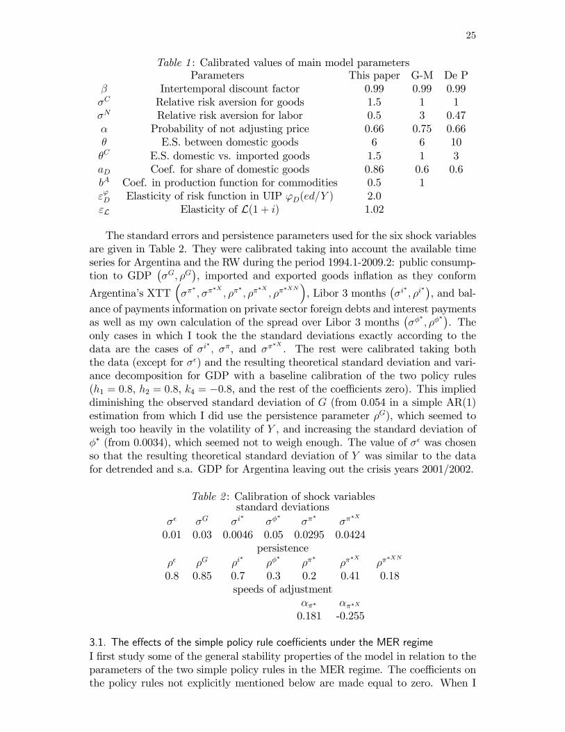
���� ���Xt�1����XN exp ����"��t � :3. Numerical solution in DynareA detailed calibration of the parameters and derivation of the NSS values of theendogenous variables can be found in Appendix 1. In this section I analyze thestabilizing role of the two policy rules under the di¤erent monetary and exchangerate regimes, mainly by studying the volatilities (standard deviations) of the mainendogenous variables in the model. I also explore the policy parameter ranges thatguarantee the Blanchard-Kahn (BK) stability conditions. Table 1 summarizes thecalibrated values of the main model parameters that are used throughout, and alsocontains some comparisons with parameter values used in two other relevant SOEmodels.17
17�E.S.�denotes �elasticity of substitution�, G_M stands for �Galí and Monacelli (2005)�, andDe P for �De Paoli (2006)�.
25
Table 1 : Calibrated values of main model parametersParameters This paper G-M De P
� Intertemporal discount factor 0.99 0.99 0.99�C Relative risk aversion for goods 1.5 1 1�N Relative risk aversion for labor 0.5 3 0.47� Probability of not adjusting price 0.66 0.75 0.66� E.S. between domestic goods 6 6 10�C E.S. domestic vs. imported goods 1.5 1 3aD Coef. for share of domestic goods 0.86 0.6 0.6bA Coef. in production function for commodities 0.5 1"'D Elasticity of risk function in UIP 'D(ed=Y ) 2.0"L Elasticity of L(1 + i) 1.02
The standard errors and persistence parameters used for the six shock variablesare given in Table 2. They were calibrated taking into account the available timeseries for Argentina and the RW during the period 1994.1-2009.2: public consump-tion to GDP
��G; �G
�, imported and exported goods in�ation as they conform
Argentina�s XTT���
�; ��
�X; ��
�; ��
�X; ��
�XN�, Libor 3 months
��i
�; �i
��, and bal-
ance of payments information on private sector foreign debts and interest paymentsas well as my own calculation of the spread over Libor 3 months
���
�; ��
��. The
only cases in which I took the the standard deviations exactly according to thedata are the cases of �i
�; ��, and ��
�X. The rest were calibrated taking both
the data (except for ��) and the resulting theoretical standard deviation and vari-ance decomposition for GDP with a baseline calibration of the two policy rules(h1 = 0:8, h2 = 0:8, k4 = �0:8, and the rest of the coe¢ cients zero). This implieddiminishing the observed standard deviation of G (from 0.054 in a simple AR(1)estimation from which I did use the persistence parameter �G), which seemed toweigh too heavily in the volatility of Y , and increasing the standard deviation of�� (from 0.0034), which seemed not to weigh enough. The value of �� was chosenso that the resulting theoretical standard deviation of Y was similar to the datafor detrended and s.a. GDP for Argentina leaving out the crisis years 2001/2002.
Table 2 : Calibration of shock variablesstandard deviations
�� �G �i�
���
���
���X
0.01 0.03 0.0046 0.05 0.0295 0.0424persistence
�� �G �i�
���
���
���X
���XN
0.8 0.85 0.7 0.3 0.2 0.41 0.18speeds of adjustment
��� ���X0.181 -0.255
3.1. The e¤ects of the simple policy rule coe¢ cients under the MER regimeI �rst study some of the general stability properties of the model in relation to theparameters of the two simple policy rules in the MER regime. The coe¢ cients onthe policy rules not explicitly mentioned below are made equal to zero. When I
26
say that a particular con�guration of parameters gives stability I mean that all therequirements for determinacy and non-explosiveness are met, including the rankcondition. In particular, there are no unit roots.1) A very general result is that if the coe¢ cient that makes the rate of nominal
appreciation respond to central bank deviations from target is zero (k4 = 0) themodel has a unit root for any value of the remaining coe¢ cients. Hence, from nowon k4 will always be di¤erent from zero in the MER regime. Let k4 = �0:8 untilfurther notice. Observe that with negative values for k4, when there are insu¢ cientreserves, and hence, etrt=Yt < R, i.e. bet + brt � bYt < 0, the CB tends to depreciatethe currency (more than in the NSS):
b�t = k4 �bet + brt � bYt� > 0:Since a purchase of IR (increase in rt) expands the money supply (ceteris paribus)one tends to associate it with a currency depreciation. But thins are more complex.First, it is the ratio between the real domestic value of IR (etrt) to GDP that mustincrease if in the initial period etrt=Yt < R. Second, that increase must takeplace in the long run, so the direction of movement may be the opposite duringa transition period. In fact, I show below that sometimes it is optimal to have apositive k4.2) I �rst look at very streamlined policy rules with no inertia, an interest rate
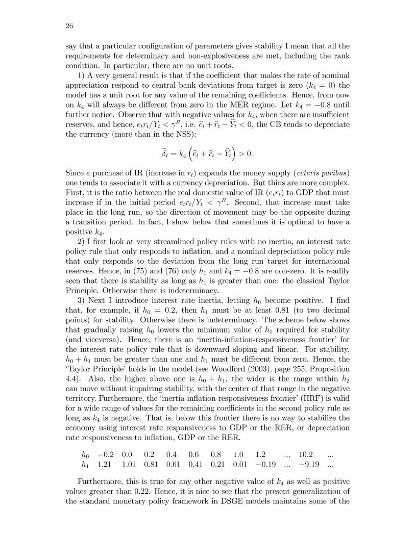
policy rule that only responds to in�ation, and a nominal depreciation policy rulethat only responds to the deviation from the long run target for internationalreserves. Hence, in (75) and (76) only h1 and k4 = �0:8 are non-zero. It is readilyseen that there is stability as long as h1 is greater than one: the classical TaylorPrinciple. Otherwise there is indeterminacy.3) Next I introduce interest rate inertia, letting h0 become positive. I �nd
that, for example, if h0 = 0:2, then h1 must be at least 0.81 (to two decimalpoints) for stability. Otherwise there is indeterminacy. The scheme below showsthat gradually raising h0 lowers the minimum value of h1 required for stability(and viceversa). Hence, there is an �inertia-in�ation-responsiveness frontier� forthe interest rate policy rule that is downward sloping and linear. For stability,h0 + h1 must be greater than one and h1 must be di¤erent from zero. Hence, the�Taylor Principle�holds in the model (see Woodford (2003), page 255, Proposition4.4). Also, the higher above one is h0 + h1, the wider is the range within h2can move without impairing stability, with the center of that range in the negativeterritory. Furthermore, the �inertia-in�ation-responsiveness frontier�(IIRF) is validfor a wide range of values for the remaining coe¢ cients in the second policy rule aslong as k4 is negative. That is, below this frontier there is no way to stabilize theeconomy using interest rate responsiveness to GDP or the RER, or depreciationrate responsiveness to in�ation, GDP or the RER.
h0 �0:2 0:0 0:2 0:4 0:6 0:8 1:0 1:2 ::: 10:2 :::h1 1:21 1:01 0:81 0:61 0:41 0:21 0:01 �0:19 ::: �9:19 :::
Furthermore, this is true for any other negative value of k4 as well as positivevalues greater than 0.22. Hence, it is nice to see that the present generalization ofthe standard monetary policy framework in DSGE models maintains some of the

27
key ingredients in the more limited, conventional, model. On the other hand, ifk4 has low positive values (less than or equal to 0.23), there is a reversal in theTaylor Principle: stability requires that h0 + h1 be less than one. Remarkably, apolicy with a positive k4 less than 0.24 (to two digits) and all the other coe¢ cientsin both policy rules equal to zero is stable. Positive values for k4 will come upbelow as optimal values for simple policy rules in the MER regime for certainCB styles. This illustrates the fact that the general model (with the MER) isconsiderably more complex (and richer) than the standard models (with either ofthe two �corner�regimes: FER or PER).4) Next I looked a little closer into the e¤ects of changing one of the two critical
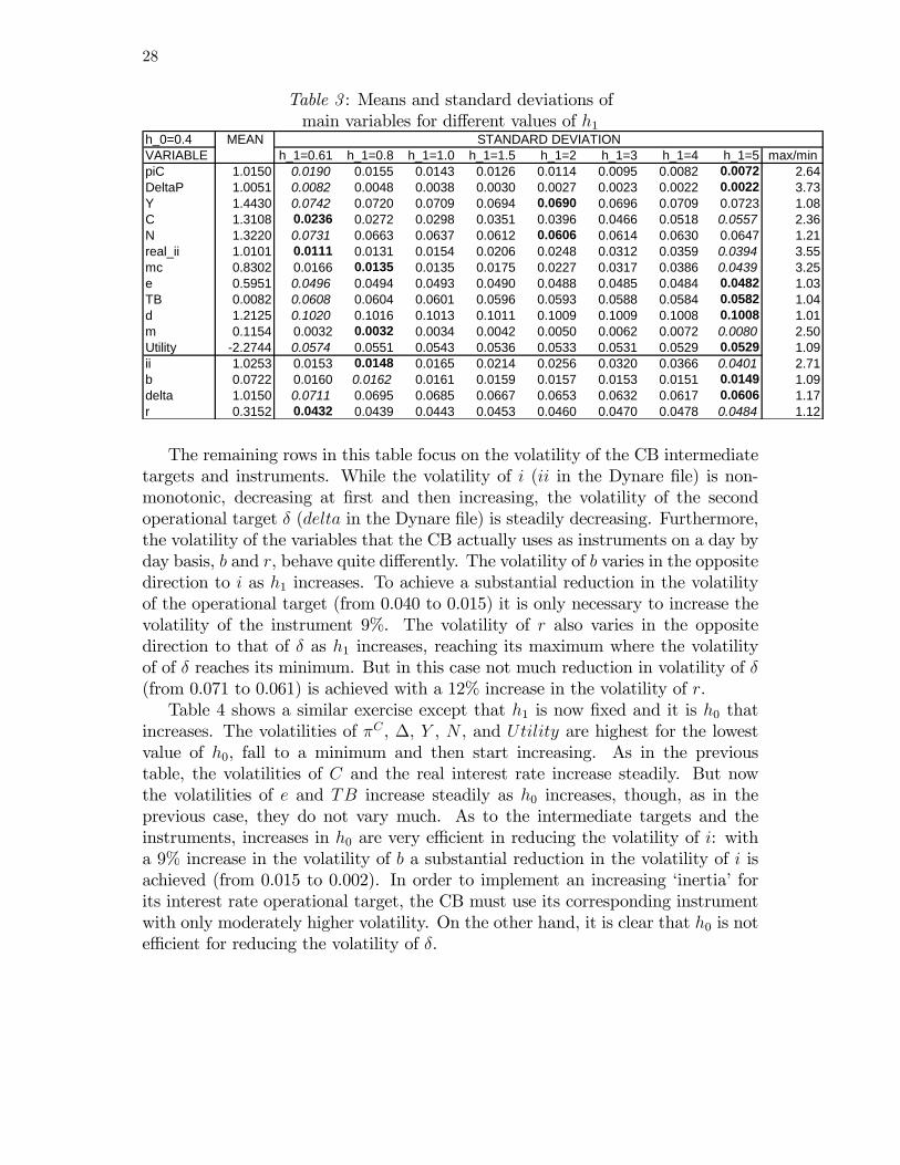
coe¢ cients h0 and h1 (keeping the rest at baseline values) on the standard devia-tions of some of the endogenous variables Central Banks typically care for.18 FirstI take a �xed value of h0 starting on the IIRF and �nd the volatilities (standarddeviations) for increasing values of h1. The results are in the Table 3, where theminimum value in each row is highlighted in bold and the maximum is in italics.The ratio between the maximum and minimum volatility is also shown in the lastcolumn. It is interesting to see that some of the volatilities of variables of interestdecrease steadily (in�ation -piC in the Dynare �le-, price dispersion -DeltaP -, theRER -e-, TB, Utility, d, �) while others increase steadily (C, real interest rate,r), and still others at �rst diminish, reach their minimum, and then increase (Y ,N , mc). Maximum volatilities are almost always in the extremes, but minimumvolatilities are more scattered.Although attention is usually focused on the volatility of Y , it is C and N
that enter the aggregate utility of households, and their volatilities respond quitedi¤erently to increases in h1. Indeed, while the volatility of C increases steadilywith h1, that of N falls up to h1 = 2 and then starts to increase. The volatilityof period utility (Utility), however, steadily diminishes as h1 increases, as does thevolatility of in�ation and price dispersion.
18Amato and Laubach (2003) do a similar analysis for the case of sticky prices and wages whenonly an interest rate rule is used.
28
Table 3 : Means and standard deviations ofmain variables for di¤erent values of h1
h_0=0.4 MEANVARIABLE h_1=0.61 h_1=0.8 h_1=1.0 h_1=1.5 h_1=2 h_1=3 h_1=4 h_1=5 max/minpiC 1.0150 0.0190 0.0155 0.0143 0.0126 0.0114 0.0095 0.0082 0.0072 2.64DeltaP 1.0051 0.0082 0.0048 0.0038 0.0030 0.0027 0.0023 0.0022 0.0022 3.73Y 1.4430 0.0742 0.0720 0.0709 0.0694 0.0690 0.0696 0.0709 0.0723 1.08C 1.3108 0.0236 0.0272 0.0298 0.0351 0.0396 0.0466 0.0518 0.0557 2.36N 1.3220 0.0731 0.0663 0.0637 0.0612 0.0606 0.0614 0.0630 0.0647 1.21real_ii 1.0101 0.0111 0.0131 0.0154 0.0206 0.0248 0.0312 0.0359 0.0394 3.55mc 0.8302 0.0166 0.0135 0.0135 0.0175 0.0227 0.0317 0.0386 0.0439 3.25e 0.5951 0.0496 0.0494 0.0493 0.0490 0.0488 0.0485 0.0484 0.0482 1.03TB 0.0082 0.0608 0.0604 0.0601 0.0596 0.0593 0.0588 0.0584 0.0582 1.04d 1.2125 0.1020 0.1016 0.1013 0.1011 0.1009 0.1009 0.1008 0.1008 1.01m 0.1154 0.0032 0.0032 0.0034 0.0042 0.0050 0.0062 0.0072 0.0080 2.50Utility 2.2744 0.0574 0.0551 0.0543 0.0536 0.0533 0.0531 0.0529 0.0529 1.09ii 1.0253 0.0153 0.0148 0.0165 0.0214 0.0256 0.0320 0.0366 0.0401 2.71b 0.0722 0.0160 0.0162 0.0161 0.0159 0.0157 0.0153 0.0151 0.0149 1.09delta 1.0150 0.0711 0.0695 0.0685 0.0667 0.0653 0.0632 0.0617 0.0606 1.17r 0.3152 0.0432 0.0439 0.0443 0.0453 0.0460 0.0470 0.0478 0.0484 1.12
STANDARD DEVIATION
The remaining rows in this table focus on the volatility of the CB intermediatetargets and instruments. While the volatility of i (ii in the Dynare �le) is non-monotonic, decreasing at �rst and then increasing, the volatility of the secondoperational target � (delta in the Dynare �le) is steadily decreasing. Furthermore,the volatility of the variables that the CB actually uses as instruments on a day byday basis, b and r, behave quite di¤erently. The volatility of b varies in the oppositedirection to i as h1 increases. To achieve a substantial reduction in the volatilityof the operational target (from 0.040 to 0.015) it is only necessary to increase thevolatility of the instrument 9%. The volatility of r also varies in the oppositedirection to that of � as h1 increases, reaching its maximum where the volatilityof of � reaches its minimum. But in this case not much reduction in volatility of �(from 0.071 to 0.061) is achieved with a 12% increase in the volatility of r.Table 4 shows a similar exercise except that h1 is now �xed and it is h0 that
increases. The volatilities of �C , �, Y , N , and Utility are highest for the lowestvalue of h0, fall to a minimum and then start increasing. As in the previoustable, the volatilities of C and the real interest rate increase steadily. But nowthe volatilities of e and TB increase steadily as h0 increases, though, as in theprevious case, they do not vary much. As to the intermediate targets and theinstruments, increases in h0 are very e¢ cient in reducing the volatility of i: witha 9% increase in the volatility of b a substantial reduction in the volatility of i isachieved (from 0.015 to 0.002). In order to implement an increasing �inertia�forits interest rate operational target, the CB must use its corresponding instrumentwith only moderately higher volatility. On the other hand, it is clear that h0 is note¢ cient for reducing the volatility of �.

29
Table 4 : Means and standard deviations ofmain variables for di¤erent values of h0
h_1=0.61 MEANVARIABLE h_0=0.4 h_0=0.6 h_0=0.8 h_0=1.0 h_0=2 h_0=3 h_0=4 h_0=5 max/minpiC 1.0150 0.0190 0.0142 0.0126 0.0118 0.0123 0.0137 0.0146 0.0152 1.61DeltaP 1.0051 0.0082 0.0033 0.0015 0.0007 0.0040 0.0056 0.0064 0.0070 11.71Y 1.4430 0.0742 0.0721 0.0710 0.0705 0.0705 0.0710 0.0713 0.0716 1.05C 1.3108 0.0236 0.0272 0.0298 0.0320 0.0381 0.0405 0.0417 0.0424 1.80N 1.3220 0.0731 0.0649 0.0620 0.0608 0.0612 0.0625 0.0633 0.0639 1.20real_ii 1.0101 0.0111 0.0119 0.0129 0.0137 0.0158 0.0165 0.0169 0.0171 1.54mc 0.8302 0.0166 0.0111 0.0094 0.0105 0.0198 0.0241 0.0263 0.0276 2.94e 0.5951 0.0496 0.0497 0.0500 0.0503 0.0512 0.0515 0.0517 0.0519 1.05TB 0.0082 0.0608 0.0610 0.0615 0.0620 0.0636 0.0643 0.0647 0.0649 1.07d 1.2125 0.1020 0.1031 0.1045 0.1058 0.1094 0.1107 0.1113 0.1117 1.10m 0.1154 0.0032 0.0027 0.0026 0.0025 0.0025 0.0025 0.0025 0.0025 1.28Utility 2.2744 0.0574 0.0543 0.0533 0.0529 0.0523 0.0523 0.0523 0.0523 1.10ii 1.0253 0.0153 0.0111 0.0096 0.0085 0.0051 0.0035 0.0027 0.0022 6.95b 0.0722 0.0160 0.0166 0.0168 0.0169 0.0172 0.0174 0.0174 0.0174 1.09delta 1.0150 0.0711 0.0698 0.0694 0.0692 0.0692 0.0695 0.0697 0.0699 1.03r 0.3152 0.0432 0.0440 0.0445 0.0447 0.0451 0.0451 0.0451 0.0452 1.05
STANDARD DEVIATION
5) Now I look at what happens when the CB changes the speed with which itseeks to attain its long run target for international reserves through its nominaldepreciation response. For this I keep h0 and h1 constant at values in the interiorof the IIRF (h0 = 0:4 and h1 = 0:8 ) while k4 gets increasingly negative, startingfrom -0.1.
Table 5 : Means and standard deviations ofmain variables for di¤erent values of k4
h_0=0.4, h_1=0.8VARIABLE MEAN k_4=0.1 k_4=0.4 k_4=0.7 k_4=1 k_4=2 k_4=3 k_4=4 k_4=5 max/minpiC 1.0150 0.0135 0.0148 0.0154 0.0157 0.0161 0.0162 0.0163 0.0163 1.21DeltaP 1.0051 0.0053 0.0049 0.0048 0.0048 0.0048 0.0048 0.0048 0.0048 1.10Y 1.4430 0.0778 0.0719 0.0720 0.0721 0.0724 0.0725 0.0725 0.0726 1.08C 1.3108 0.0282 0.0272 0.0272 0.0272 0.0273 0.0273 0.0273 0.0273 1.04N 1.3220 0.0689 0.0664 0.0663 0.0664 0.0664 0.0665 0.0665 0.0665 1.04real_ii 1.0101 0.0102 0.0121 0.0130 0.0134 0.0141 0.0144 0.0146 0.0147 1.44mc 0.8302 0.0182 0.0140 0.0136 0.0134 0.0132 0.0131 0.0131 0.0131 1.39e 0.5951 0.0496 0.0492 0.0494 0.0495 0.0497 0.0498 0.0499 0.0499 1.01TB 0.0082 0.0722 0.0593 0.0601 0.0608 0.0619 0.0624 0.0626 0.0628 1.22d 1.2125 0.1353 0.1101 0.1029 0.0997 0.0960 0.0948 0.0942 0.0938 1.44m 0.1154 0.0033 0.0032 0.0032 0.0032 0.0032 0.0032 0.0032 0.0032 1.03Utility 2.2744 0.0557 0.0549 0.0551 0.0552 0.0553 0.0554 0.0554 0.0554 1.01ii 1.0253 0.0151 0.0147 0.0148 0.0149 0.0149 0.0150 0.0150 0.0150 1.03b 0.0722 0.0919 0.0282 0.0178 0.0140 0.0110 0.0107 0.0108 0.0109 8.59delta 1.0150 0.0504 0.0640 0.0686 0.0709 0.0740 0.0751 0.0757 0.0761 1.51r 0.3152 0.1700 0.0645 0.0468 0.0397 0.0319 0.0295 0.0284 0.0278 6.12
STANDARD DEVIATION
Several of the variables of interest have minimum volatilities for k4 in the range�0:1= � 0:7 . On the other hand, �, mc, d, and m have lowest volatilities atk4 = �5. As k4 gets less negative (going from right to left in Table 5) an increas-ingly volatile use of the instrument (r) progressively reduces the volatility of theoperational target (�). It also has the e¤ect of reducing the volatility of in�ation.Surprisingly, it also implies a slight increase in the volatility of price dispersion.Furthermore, the volatility of the other instrument (b) also increases, without asigni�cant e¤ect on the volatility of the other operational target (i).

30
6) To get a feeling for the range within I could move each policy rule coe¢ cient,I started from a baseline calibration for the coe¢ cients in the two policy feedbackrules well within the IIRF frontier and looked for the intervals within which each ofthe coe¢ cients could be moved individually (leaving the rest at the baseline value)without impairing stability. I restricted my search to two decimal points accuracyand only checked for parameter values below 10 in absolute value. The followingis the baseline calibration for this exercise:
Baseline calibrationh0 h1 h2 h3 k0 k1 k2 k3 k40:8 0:8 0:0 0:0 0:0 0:0 0:0 0:0 �0:8
The results for the three policy regimes are in the Table 6. Starting with thegeneral MER regime, both of the inertial coe¢ cient intervals of stability are quitewide, both going into high superinertial levels (of 10 and 4.48 for the interest rateand depreciation rate rules, respectively). Because unity is included in the feasibleintervals for h0 and k0, one or both of the simple policy rules can be implemented asthe feedback response of the �rst di¤erence (in the interest rate or the depreciationrate, respectively) to the various arguments on the r.h.s. In the case of the interestrate rule, there are no upper bounds for the reactions to in�ation or the RER, but,perhaps surprisingly, there is an upper bound of only 1.04 for the response to GDP.There is much more room for an accommodating policy of diminishing (raising)the interest rate (up to -3.69) when GDP is high (low). In the case of the nominaldepreciation rule, there are no upper or lower bounds for the reactions to in�ationor GDP, and an upper bound of 9.12 for the reaction to the RER. In the case ofk4, the only restriction is that it must be outside of a small interval around zero,which is mostly on the positive side. The fact that there is a comparatively lowupper bound for the interest rate response to GDP while there is no bound for thenominal depreciation response to the same variable is quite interesting, since thestabilization of GDP is, of course, of primary interest in most CBs (along with thestabilization of in�ation).
Table 6 : Stability ranges for individual coe¢ cients of policy rulesMER FER PER
Interest rate ruleh0 2 [0:21; 10] [0:21; 10]h1 2 [0:21; 10] [0:21; 10]h2 2 [�3:69; 1:04] [�3:54; 1:03]h3 2 [�8:14; 10] [�6:89; 4:63]
Nominal depreciation rulek0 2 [�4:55; 4:48] [�1:32; 0:67]k1 2 [�10; 10] [�10; 10]k2 2 [�10; 10] [�1:16; 1:67]k3 2 [�10; 9:12] [�1:77; 2:82]k4 2 [�10;�0:01] [ [0:23; 10] [�0:95; 2:44]
The FER regime shows stability ranges that are very similar to those of the �rstpolicy rule of the MER regime. There is a narrowing of the range in the case of h3.
31
The narrowing of the range of stability is more signi�cant in the case of the PERregime, especially in the cases of k2, k3, and k4. On the other hand, in the PERregime the stability range for k4 includes 0, indicating that the need to respond toa target for international reserves is only valid in the more general MER regime.Because GDP is typically available with a signi�cant lag, it is of interest to see
how these stability ranges are altered when the policy rules respond to output witha one quarter lag. Hence, the exercise was repeated by replacing Yt with Yt�1 inboth simple policy rules (including the IRs ratio to GDP). The resulting stabilityranges are quite similar. For both the MER and FER regimes there is again noupper bound for h0 and h1, and in this case there is no lower bound for h2, whereasthe same upper bound subsists. There is no lower bound for h3 in the case of theMER regime, and an increase in the upper bound to 5:99 in the FER regime. Thestability ranges for the ki remain almost unaltered in the case of the MER regime.In the PER regime, however, k1 is bounded above (by 0:67) whereas k2 is not.Also, the stability range for k3 is widened to [�1:77; 2:82] and the lower bound fork4 becomes �2:45.Leaving behind the baseline calibration, it is interesting to verify that in the
PER case there is stability when all the coe¢ cients are zero (kj = 0; j = 0; 1; 2; 3; 4).In this case the policy rule is to intervene in the FX market su¢ ciently to maintainthe nominal exchange rate �xed at the existing level, letting the economy run itscourse, and not worrying about international reserves.19
7) The relatively narrow range of stability for the coe¢ cient on the interest rateresponse to GDP deviations (h2) in the MER case, along with the boundless rangeof stability for the corresponding coe¢ cient in the second policy rule (k2), naturallyraises the question of the e¤ects of the latter coe¢ cient on the volatilities. Table 7shows these e¤ects. Most the variables reach minimum volatilities for non-positivevalues of k2. And for a number of very signi�cant variables such as �, Y , C, N , m,and Utility, the minimum is reached for highly negative values of k2 (-10 or -8).Indeed, the lowest volatility of Y , N , and Utility is lower than the lowest volatilitythey achieve, respectively, in any of the analogous tables above. Hence, reducingthe rate of nominal depreciation (or perhaps even appreciating the currency) whenGDP is above its NSS level has a very important stabilizing role for most of thevariables of interest. Notice that this implies using both instruments with highvolatility.
19However, one must bear in mind that here the nominal and real exchange rates are (inspirit) multilateral. If we modeled a multicountry RW, the nominal exchange rate would be thedomestic currency price of a basket of the nominal exchange rates of the SOE�s trade partners,with weights equal to the shares in trade. Hence, our peg is completely di¤erent from peggingagainst the currency of a country with which only a small part of the SOE�s trade is done (aswas the case of Argentina�s ill fated �Convertibility�).
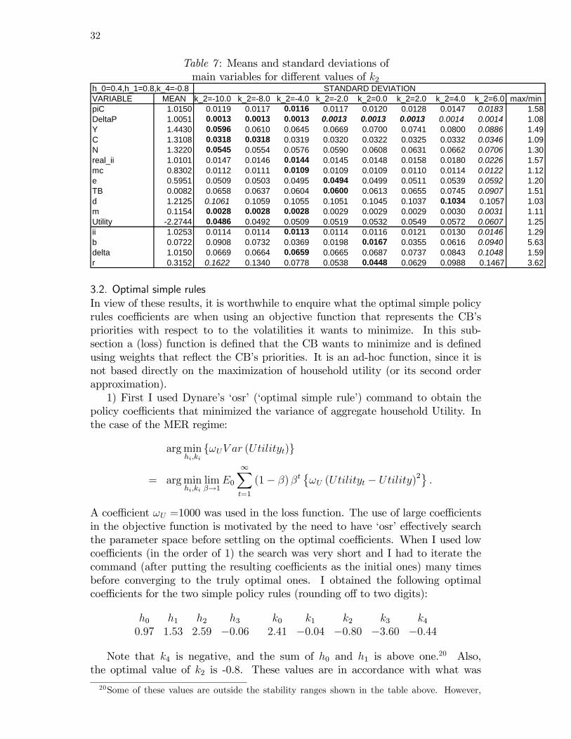
32
Table 7 : Means and standard deviations ofmain variables for di¤erent values of k2
h_0=0.4,h_1=0.8,k_4=0.8VARIABLE MEAN k_2=10.0 k_2=8.0 k_2=4.0 k_2=2.0 k_2=0.0 k_2=2.0 k_2=4.0 k_2=6.0 max/minpiC 1.0150 0.0119 0.0117 0.0116 0.0117 0.0120 0.0128 0.0147 0.0183 1.58DeltaP 1.0051 0.0013 0.0013 0.0013 0.0013 0.0013 0.0013 0.0014 0.0014 1.08Y 1.4430 0.0596 0.0610 0.0645 0.0669 0.0700 0.0741 0.0800 0.0886 1.49C 1.3108 0.0318 0.0318 0.0319 0.0320 0.0322 0.0325 0.0332 0.0346 1.09N 1.3220 0.0545 0.0554 0.0576 0.0590 0.0608 0.0631 0.0662 0.0706 1.30real_ii 1.0101 0.0147 0.0146 0.0144 0.0145 0.0148 0.0158 0.0180 0.0226 1.57mc 0.8302 0.0112 0.0111 0.0109 0.0109 0.0109 0.0110 0.0114 0.0122 1.12e 0.5951 0.0509 0.0503 0.0495 0.0494 0.0499 0.0511 0.0539 0.0592 1.20TB 0.0082 0.0658 0.0637 0.0604 0.0600 0.0613 0.0655 0.0745 0.0907 1.51d 1.2125 0.1061 0.1059 0.1055 0.1051 0.1045 0.1037 0.1034 0.1057 1.03m 0.1154 0.0028 0.0028 0.0028 0.0029 0.0029 0.0029 0.0030 0.0031 1.11Utility 2.2744 0.0486 0.0492 0.0509 0.0519 0.0532 0.0549 0.0572 0.0607 1.25ii 1.0253 0.0114 0.0114 0.0113 0.0114 0.0116 0.0121 0.0130 0.0146 1.29b 0.0722 0.0908 0.0732 0.0369 0.0198 0.0167 0.0355 0.0616 0.0940 5.63delta 1.0150 0.0669 0.0664 0.0659 0.0665 0.0687 0.0737 0.0843 0.1048 1.59r 0.3152 0.1622 0.1340 0.0778 0.0538 0.0448 0.0629 0.0988 0.1467 3.62
STANDARD DEVIATION
3.2. Optimal simple rulesIn view of these results, it is worthwhile to enquire what the optimal simple policyrules coe¢ cients are when using an objective function that represents the CB�spriorities with respect to to the volatilities it wants to minimize. In this sub-section a (loss) function is de�ned that the CB wants to minimize and is de�nedusing weights that re�ect the CB�s priorities. It is an ad-hoc function, since it isnot based directly on the maximization of household utility (or its second orderapproximation).1) First I used Dynare�s �osr�(�optimal simple rule�) command to obtain the
policy coe¢ cients that minimized the variance of aggregate household Utility. Inthe case of the MER regime:
argminhi;ki
f!UV ar (Utilityt)g
= argminhi;ki
lim�!1
E0
1Xt=1
(1� �) �t�!U (Utilityt � Utility)2
:
A coe¢ cient !U =1000 was used in the loss function. The use of large coe¢ cientsin the objective function is motivated by the need to have �osr�e¤ectively searchthe parameter space before settling on the optimal coe¢ cients. When I used lowcoe¢ cients (in the order of 1) the search was very short and I had to iterate thecommand (after putting the resulting coe¢ cients as the initial ones) many timesbefore converging to the truly optimal ones. I obtained the following optimalcoe¢ cients for the two simple policy rules (rounding o¤ to two digits):
h0 h1 h2 h3 k0 k1 k2 k3 k40:97 1:53 2:59 �0:06 2:41 �0:04 �0:80 �3:60 �0:44
Note that k4 is negative, and the sum of h0 and h1 is above one.20 Also,the optimal value of k2 is -0.8. These values are in accordance with what was
20Some of these values are outside the stability ranges shown in the table above. However,

33
obtained above. Under our simple rules, and assuming that the policymakers wishto reduce the variance of the utility of households, it is optimal to react stronglyand positively to in�ation and GDP in the interest rate rule and strongly andnegatively to the RER in the nominal depreciation rule. A deviation of 1% inin�ation above its target value here commands an increase of 1.5 p.p. in theinterest rate (assuming it was at the NSS level the previous period) and a slightreduction of 0.04 p.p. in the rate of nominal depreciation (assuming it was at theNSS level the previous period). And a deviation of 1% in GDP above its NSSvalue commands an increase in the interest rate of 2.6 p.p. and a reduction of 0.8p.p. in the rate of nominal depreciation. On the other hand, a deviation of 1%in the RER above its NSS value commands a tiny reduction in the interest rate(of 0.06 p.p.) and a signi�cant reduction in the rate of nominal depreciation of3.6 p.p. The latter seems quite natural: if the currency is weak in real terms (eis high), it is optimal to depreciate less. Finally, it is optimal to make strong useof policy inertia in both rules (superinertial in the case of the second policy rule)even though no CB preference for such policies has been assumed.Table 8 shows the standard deviations of the main endogenous variables when
using these optimal simple rules.
Table 8 : Means and standard deviations of main variables underoptimal simple rules that minimize the variance of Utility
VARIABLE MEAN Std.Dev. Std.Dev./MeanpiC 1.015 0.065 0.06DeltaP 1.005 0.044 0.04Y 1.443 0.052 0.04C 1.311 0.036 0.03N 1.322 0.033 0.02real_ii 1.010 0.020 0.02mc 0.830 0.037 0.04e 0.595 0.037 0.06TB 0.008 0.058 7.11d 1.213 0.131 0.11m 0.115 0.005 0.05Utility 2.274 0.032 0.01ii 1.025 0.053 0.05b 0.072 0.102 1.41delta 1.015 0.079 0.08r 0.315 0.182 0.58
First, notice how small the standard deviation of Utility is. While the fourtables above all had standard deviations above 0.0486, the �osr�routine reduced itto 0.032. Second, it is noteworthy that minimizing the volatility of Utility actuallyimplies having substantial volatilities in many of the variables that ad-hoc CB lossfunctions usually try to minimize. While the highest s.d. of consumer in�ation inthe above four tables was 0.019, it is 0.065 when this optimal simple policy rule is
that range was obtained keeping all the other coe¢ cients at their baseline levels, which is notdone here. Dynare�s osr search changes direction whenever it goes into parameter values that donot comply with the Blanchard and Kahn conditions. In some cases, the search engine tended toobtain minor gains in loss with exceedingly high coe¢ cients (in absolute value, in the hundredsor thousands) when using some initializations. I always ignored such gains and kept to the moremoderate coe¢ cient values.

34
used. The contrast with the price dispersion variable is even greater. The highestabove was 0.008 and now it is 0.044.2) Few CBs actually use models in which the explicit goal of the policymaker
has to do with household utility. This is probably due to the fact that mostmodels misrepresent reality in ways that CBs cannot take for granted: they assumehomogenous households (except possibly for the heterogeneity derived from wagesetting in a monopolistically competitive setting). The usual target variables ofCB loss functions are in�ation and GDP, and there is usually some explicit distastefor excessive movement in the operational target variable (the interest rate). This,of course, also brushes away, though in a di¤erent way, the incidence of CB actionson di¤erent sectors of the economy and di¤erent factor incomes. However, whereasaggregate household utility is an abstract concept because it is known that themodel is misspeci�ed in the dimension of household heterogeneity, variables likein�ation, GDP, or the RER, have clear empirical counterparts that are very presentin the minds of policymakers when they make decisions. Hence, I now repeatthe above exercise assuming that the CB minimizes a linear combination of thevariances of its target variables:
argminhi;ki
�!�V ar
��Ct�+ !Y V ar (Yt) + !eV ar (et) + !rV ar (rt)
+!�iV ar (�it) + !��V ar (��t)g
Aside from the usual terms (with weights !�, !Y , !�i), this loss function alsoallows for CB preferences with respect to the variances of the RER, of the CBsIRs, and of changes in the rate of nominal depreciation (with weights !e, !r, !��).In Table 9 I de�ne six di¤erent CB styles (or preferences: A-F) according to thecombinations of weights in each. In all of them I have given the same weight tothe changes in each of the operational targets (50), and avoided zeros giving aweight of 1 to target variables with no importance. Hence, in style A only in�ationmatters and in style B only GDP matters, whereas both matter equally in styleC. In style D (F) the real exchange rate (international reserves) matters as muchas in�ation and GDP. Finally, in style F in�ation, GDP, the RER and the IRs allmatter equally.
Table 9 : De�nition of CB stylesWeights Styles
A B C D E F!� 100 1 100 100 100 100!Y 1 100 100 100 100 100!e 1 1 1 100 1 100!r 1 1 1 1 100 100!�i 50 50 50 50 50 50!�� 50 50 50 50 50 50
With Dynare�s �osr�command I obtained the optimal simple policy rules foreach of the CB styles in each of the interest and exchange regimes. The coe¢ cientsare shown in Table 10:
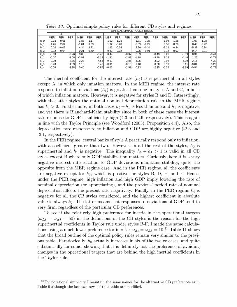
35
Table 10 : Optimal simple policy rules for di¤erent CB styles and regimes
MER FER PER MER FER PER MER FER PER MER FER PER MER FER PER MER FER PERh_0 0.33 0.01 1.86 1.17 1.63 1.28 1.71 1.28 1.94 1.28 1.97 1.28h_1 1.26 2.04 1.01 0.39 1.92 0.20 2.09 0.22 0.56 0.20 0.49 0.22h_2 0.02 0.05 4.34 3.72 1.43 0.34 2.56 0.34 5.24 0.34 5.37 0.34h_3 0.12 0.04 0.21 0.40 0.82 0.02 0.05 0.01 0.14 0.02 0.14 0.01k_0 0.03 0.26 3.08 0.47 0.44 0.37 3.39 0.43 0.26 0.39 0.34 0.41k_1 0.07 2.08 3.92 2.13 1.31 2.82 1.18 3.70 1.28 4.46 1.25 3.71k_2 0.08 2.36 2.28 4.66 0.12 3.85 3.05 3.92 2.04 5.09 2.16 4.32k_3 0.43 1.09 1.18 0.46 0.91 0.10 1.40 0.08 0.16 0.11 0.04 0.22k_4 0.08 2.18 0.40 0.87 0.06 2.57 0.13 2.35 0.74 3.29 0.84 2.74
E FOPTIMAL SIMPLE POLICY RULES
A B C D
The inertial coe¢ cient for the interest rate (h0) is superinertial in all stylesexcept A, in which only in�ation matters. In the MER regime, the interest rateresponse to in�ation deviations (h1) is greater than one in styles A and C, in bothof which in�ation matters. However, it is negative for styles B and D. Interestingly,with the latter styles the optimal nominal depreciation rule in the MER regimehas k4 > 0. Furthermore, in both cases h0+ h1 is less than one and h1 is negative,and yet there is Blanchard-Kahn stability since in both of these cases the interestrate response to GDP is su¢ ciently high (4.3 and 2.6, respectively). This is againin line with the Taylor Principle (see Woodford (2003), Proposition 4.4). Also, thedepreciation rate response to to in�ation and GDP are highly negative (-2.3 and-3.1, respectively).In the FER regime, central banks of style A practically respond only to in�ation,
with a coe¢ cient greater than two. However, in all the rest of the styles, h0 issuperinertial and h1 is negative. The inequality h0 + h1 > 1 is valid in all CBstyles except B where only GDP stabilization matters. Curiously, here it is a verynegative interest rate reaction to GDP deviations maintains stability, quite theopposite from the MER regime case. And in the PER regime, all the coe¢ cientsare negative except for k3, which is positive for styles B, D, E, and F. Hence,under the PER regime, high in�ation and high GDP imply lowering the rate ofnominal depreciation (or appreciating), and the previous�period rate of nominaldepreciation a¤ects the present rate negatively. Finally, in the PER regime k4 isnegative for all the CB styles considered, and the highest coe¢ cient in absolutevalue is always k2. The latter means that responses to deviations of GDP tend tovery �rm, regardless of the particular CB preferences.To see if the relatively high preference for inertia in the operational targets
(!�i = !�� = 50) in the de�nitions of the CB styles is the reason for the highsuperinertial coe¢ cients in Taylor rule under styles B-F, I made the same calcula-tions using a much lower preference for inertia: !�i = !�� = 10.21 Table 11 showsthat the broad outline of the optimal policy rules remain very similar to the previ-ous table. Paradoxically, h0 actually increases in six of the twelve cases, and quitesubstantially for some, showing that it is de�nitely not the preference of avoidingchanges in the operational targets that are behind the high inertial coe¢ cients inthe Taylor rule.
21For notational simplicity I maintain the same names for the alternative CB preferences as inTable 9 although the last two rows of that table are modi�ed.
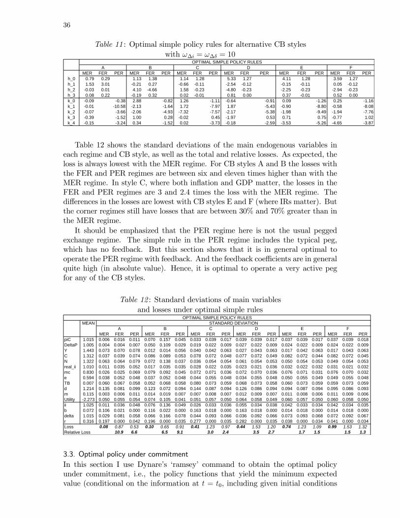
36
Table 11 : Optimal simple policy rules for alternative CB styleswith !�i = !�� = 10
MER FER PER MER FER PER MER FER PER MER FER PER MER FER PER MER FER PERh_0 0.79 0.29 1.13 1.38 1.14 1.28 5.33 1.27 4.11 1.28 3.59 1.27h_1 1.53 3.01 0.21 0.27 0.66 0.11 2.54 0.12 0.15 0.11 0.05 0.12h_2 0.03 0.01 4.10 4.66 1.58 0.23 4.80 0.23 2.25 0.23 2.94 0.23h_3 0.08 0.22 0.19 0.32 0.02 0.01 0.81 0.00 0.37 0.01 0.52 0.00k_0 0.09 0.38 2.88 0.82 1.26 1.11 0.64 0.91 0.09 1.26 0.25 1.16k_1 0.01 10.58 2.13 1.64 1.72 7.97 1.87 5.43 0.90 8.80 0.58 8.08k_2 0.07 3.66 2.06 4.93 7.32 7.57 2.17 5.38 1.98 9.49 1.94 7.76k_3 0.39 1.52 1.00 0.28 0.02 0.45 1.97 0.53 0.71 0.75 0.77 1.02k_4 0.15 3.24 0.34 1.52 0.02 3.73 0.18 2.59 3.53 5.26 4.65 3.87
E FA B C DOPTIMAL SIMPLE POLICY RULES
Table 12 shows the standard deviations of the main endogenous variables ineach regime and CB style, as well as the total and relative losses. As expected, theloss is always lowest with the MER regime. For CB styles A and B the losses withthe FER and PER regimes are between six and eleven times higher than with theMER regime. In style C, where both in�ation and GDP matter, the losses in theFER and PER regimes are 3 and 2.4 times the loss with the MER regime. Thedi¤erences in the losses are lowest with CB styles E and F (where IRs matter). Butthe corner regimes still have losses that are between 30% and 70% greater than inthe MER regime.It should be emphasized that the PER regime here is not the usual pegged
exchange regime. The simple rule in the PER regime includes the typical peg,which has no feedback. But this section shows that it is in general optimal tooperate the PER regime with feedback. And the feedback coe¢ cients are in generalquite high (in absolute value). Hence, it is optimal to operate a very active pegfor any of the CB styles.
Table 12 : Standard deviations of main variablesand losses under optimal simple rules
MEAN
MER FER PER MER FER PER MER FER PER MER FER PER MER FER PER MER FER PERpiC 1.015 0.006 0.016 0.011 0.070 0.157 0.045 0.033 0.039 0.017 0.039 0.039 0.017 0.037 0.039 0.017 0.037 0.039 0.018DeltaP 1.005 0.004 0.004 0.007 0.050 0.109 0.029 0.019 0.022 0.009 0.027 0.022 0.009 0.024 0.022 0.009 0.024 0.022 0.009Y 1.443 0.073 0.070 0.078 0.012 0.014 0.056 0.040 0.042 0.063 0.027 0.043 0.063 0.017 0.042 0.063 0.017 0.043 0.063C 1.312 0.037 0.039 0.074 0.086 0.089 0.053 0.078 0.072 0.048 0.077 0.072 0.049 0.082 0.072 0.044 0.082 0.072 0.045N 1.322 0.063 0.064 0.079 0.072 0.138 0.037 0.036 0.054 0.054 0.061 0.054 0.053 0.050 0.054 0.053 0.049 0.054 0.053real_ii 1.010 0.011 0.035 0.052 0.017 0.035 0.035 0.028 0.022 0.035 0.023 0.021 0.036 0.032 0.022 0.032 0.031 0.021 0.032mc 0.830 0.026 0.025 0.069 0.079 0.092 0.045 0.072 0.071 0.036 0.072 0.070 0.036 0.076 0.071 0.031 0.076 0.070 0.032e 0.594 0.038 0.052 0.048 0.037 0.052 0.048 0.044 0.055 0.048 0.034 0.055 0.048 0.050 0.055 0.049 0.049 0.055 0.048TB 0.007 0.060 0.067 0.058 0.052 0.068 0.058 0.080 0.073 0.059 0.068 0.073 0.058 0.060 0.073 0.059 0.059 0.073 0.059d 1.214 0.135 0.081 0.099 0.123 0.072 0.094 0.144 0.087 0.094 0.126 0.086 0.094 0.094 0.087 0.094 0.095 0.086 0.093m 0.115 0.003 0.006 0.011 0.014 0.019 0.007 0.007 0.008 0.007 0.012 0.009 0.007 0.011 0.008 0.006 0.011 0.009 0.006Utility 2.273 0.050 0.055 0.054 0.074 0.105 0.041 0.051 0.057 0.050 0.064 0.058 0.049 0.060 0.057 0.050 0.060 0.058 0.050ii 1.025 0.011 0.036 0.048 0.076 0.136 0.049 0.026 0.033 0.036 0.055 0.034 0.038 0.042 0.033 0.034 0.042 0.034 0.035b 0.072 0.106 0.021 0.000 0.116 0.022 0.000 0.163 0.018 0.000 0.163 0.018 0.000 0.014 0.018 0.000 0.014 0.018 0.000delta 1.015 0.029 0.081 0.058 0.066 0.166 0.078 0.044 0.093 0.066 0.036 0.092 0.066 0.073 0.093 0.068 0.072 0.092 0.067r 0.316 0.197 0.000 0.042 0.196 0.000 0.035 0.277 0.000 0.035 0.282 0.000 0.035 0.038 0.000 0.034 0.041 0.000 0.034Loss 0.08 0.87 0.53 0.10 0.65 0.91 0.41 1.23 0.97 0.44 1.53 1.20 0.74 1.23 1.09 0.99 1.53 1.32Relative Loss 10.9 6.6 6.5 9.1 3.0 2.4 3.5 2.7 1.7 1.5 1.5 1.3
OPTIMAL SIMPLE POLICY RULESSTANDARD DEVIATION
A B C D E F
3.3. Optimal policy under commitmentIn this section I use Dynare�s �ramsey� command to obtain the optimal policyunder commitment, i.e., the policy functions that yield the minimum expectedvalue (conditional on the information at t = t0, including given initial conditions
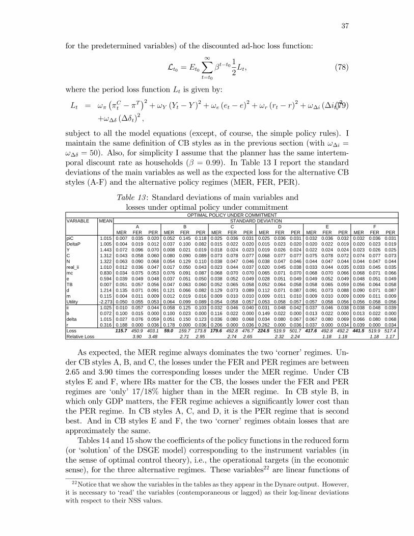
37
for the predetermined variables) of the discounted ad-hoc loss function:
Lt0 = Et01Xt=t0
�t�t01
2Lt, (78)
where the period loss function Lt is given by:
Lt = !���Ct � �T
�2+ !Y (Yt � Y )2 + !e (et � e)2 + !r (rt � r)2 + !�i (�it)2(79)
+!�� (��t)2 ;
subject to all the model equations (except, of course, the simple policy rules). Imaintain the same de�nition of CB styles as in the previous section (with !�i =!�� = 50). Also, for simplicity I assume that the planner has the same intertem-poral discount rate as households (� = 0:99). In Table 13 I report the standarddeviations of the main variables as well as the expected loss for the alternative CBstyles (A-F) and the alternative policy regimes (MER, FER, PER).
Table 13 : Standard deviations of main variables andlosses under optimal policy under commitment
VARIABLE MEAN
MER FER PER MER FER PER MER FER PER MER FER PER MER FER PER MER FER PERpiC 1.015 0.007 0.035 0.020 0.052 0.145 0.118 0.025 0.036 0.031 0.025 0.036 0.031 0.032 0.036 0.032 0.032 0.036 0.031DeltaP 1.005 0.004 0.019 0.012 0.037 0.100 0.082 0.015 0.022 0.020 0.015 0.023 0.020 0.020 0.022 0.019 0.020 0.023 0.019Y 1.443 0.072 0.096 0.070 0.008 0.021 0.019 0.018 0.024 0.023 0.019 0.026 0.024 0.022 0.024 0.024 0.023 0.026 0.025C 1.312 0.043 0.058 0.060 0.080 0.090 0.089 0.073 0.078 0.077 0.068 0.077 0.077 0.075 0.078 0.072 0.074 0.077 0.073N 1.322 0.063 0.090 0.068 0.054 0.129 0.110 0.038 0.047 0.046 0.038 0.047 0.046 0.044 0.047 0.044 0.044 0.047 0.044real_ii 1.010 0.012 0.036 0.047 0.017 0.050 0.043 0.023 0.044 0.037 0.020 0.045 0.038 0.033 0.044 0.035 0.033 0.045 0.035mc 0.830 0.034 0.075 0.053 0.076 0.091 0.087 0.068 0.070 0.070 0.065 0.071 0.070 0.068 0.070 0.066 0.068 0.071 0.066e 0.594 0.039 0.049 0.048 0.037 0.051 0.050 0.038 0.052 0.049 0.028 0.051 0.049 0.049 0.052 0.049 0.048 0.051 0.049TB 0.007 0.051 0.057 0.056 0.047 0.063 0.060 0.052 0.065 0.058 0.052 0.064 0.058 0.058 0.065 0.059 0.056 0.064 0.058d 1.214 0.135 0.071 0.091 0.121 0.066 0.082 0.129 0.073 0.089 0.112 0.071 0.087 0.091 0.073 0.088 0.090 0.071 0.087m 0.115 0.004 0.011 0.009 0.012 0.019 0.016 0.009 0.010 0.010 0.009 0.011 0.010 0.009 0.010 0.009 0.009 0.011 0.009Utility 2.273 0.050 0.055 0.053 0.064 0.099 0.089 0.054 0.058 0.057 0.053 0.058 0.057 0.057 0.058 0.056 0.056 0.058 0.056ii 1.025 0.010 0.057 0.044 0.058 0.125 0.103 0.032 0.046 0.040 0.031 0.048 0.042 0.037 0.046 0.038 0.038 0.048 0.039b 0.072 0.100 0.015 0.000 0.100 0.023 0.000 0.116 0.022 0.000 0.149 0.022 0.000 0.013 0.022 0.000 0.013 0.022 0.000delta 1.015 0.027 0.076 0.059 0.051 0.150 0.123 0.036 0.080 0.068 0.034 0.080 0.067 0.067 0.080 0.069 0.066 0.080 0.068r 0.316 0.188 0.000 0.036 0.178 0.000 0.036 0.206 0.000 0.036 0.262 0.000 0.036 0.037 0.000 0.034 0.039 0.000 0.034Loss 115.7 450.9 403.1 59.0 159.7 173.8 179.6 492.8 476.7 224.5 519.9 501.7 417.6 492.8 492.2 441.5 519.9 517.4Relative Loss 3.90 3.48 2.71 2.95 2.74 2.65 2.32 2.24 1.18 1.18 1.18 1.17
OPTIMAL POLICY UNDER COMMITMENTSTANDARD DEVIATION
A B C D E F
As expected, the MER regime always dominates the two �corner�regimes. Un-der CB styles A, B, and C, the losses under the FER and PER regimes are between2.65 and 3.90 times the corresponding losses under the MER regime. Under CBstyles E and F, where IRs matter for the CB, the losses under the FER and PERregimes are �only� 17/18% higher than in the MER regime. In CB style B, inwhich only GDP matters, the FER regime achieves a signi�cantly lower cost thanthe PER regime. In CB styles A, C, and D, it is the PER regime that is secondbest. And in CB styles E and F, the two �corner�regimes obtain losses that areapproximately the same.Tables 14 and 15 show the coe¢ cients of the policy functions in the reduced form
(or �solution�of the DSGE model) corresponding to the instrument variables (inthe sense of optimal control theory), i.e., the operational targets (in the economicsense), for the three alternative regimes. These variables22 are linear functions of
22Notice that we show the variables in the tables as they appear in the Dynare output. However,it is necessary to �read�the variables (contemporaneous or lagged) as their log-linear deviationswith respect to their NSS values.
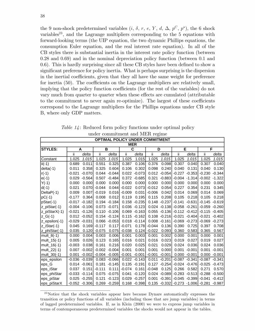
38
the 9 non-shock predetermined variables (i, �, r, e, Y , d, �, pC , p�), the 6 shockvariables23, and the Lagrange multipliers corresponding to the 5 equations withforward-looking terms (the UIP equation, the two dynamic Phillips equations, theconsumption Euler equation, and the real interest rate equation). In all of theCB styles there is substantial inertia in the interest rate policy function (between0.28 and 0.69) and in the nominal depreciation policy function (between 0.1 and0.6). This is hardly surprising since all these CB styles have been de�ned to show asigni�cant preference for policy inertia. What is perhaps surprising is the dispersionin the inertial coe¢ cients, given that they all have the same weight for preferencefor inertia (50). The coe¢ cients on the Lagrange multipliers are relatively small,implying that the policy function coe¢ cients (for the rest of the variables) do notvary much from quarter to quarter when these e¤ects are cumulated (attributableto the commitment to never again re-optimize). The largest of these coe¢ cientscorrespond to the Lagrange multipliers for the Phillips equations under CB styleB, where only GDP matters.
Table 14 : Reduced form policy functions under optimal policyunder commitment and MER regime
STYLES:ii delta ii delta ii delta ii delta ii delta ii delta
Constant 1.025 1.015 1.025 1.015 1.025 1.015 1.025 1.015 1.025 1.015 1.025 1.015ii(1) 0.689 0.011 0.551 0.325 0.387 0.106 0.376 0.098 0.307 0.040 0.307 0.040delta(1) 0.011 0.358 0.325 0.604 0.106 0.302 0.098 0.240 0.040 0.131 0.040 0.130r(1) 0.021 0.070 0.044 0.044 0.022 0.073 0.012 0.054 0.227 0.353 0.230 0.344e(1) 0.029 0.564 0.507 0.484 0.372 0.685 0.321 0.883 0.004 1.314 0.002 1.322Y(1) 0.000 0.000 0.000 0.000 0.000 0.000 0.000 0.000 0.000 0.000 0.000 0.000d(1) 0.021 0.070 0.044 0.044 0.022 0.073 0.012 0.054 0.227 0.354 0.231 0.345DeltaP(1) 0.009 0.007 0.019 0.016 0.009 0.031 0.006 0.042 0.014 0.069 0.014 0.069pC(1) 0.177 0.364 0.008 0.012 0.119 0.195 0.115 0.208 0.105 0.218 0.105 0.218pStar(1) 0.017 0.182 0.194 0.184 0.158 0.235 0.148 0.237 0.141 0.631 0.145 0.619z_piStar(1) 0.004 0.106 0.073 0.071 0.036 0.123 0.024 0.138 0.058 0.261 0.059 0.260z_piStarX(1) 0.021 0.126 0.110 0.106 0.069 0.163 0.055 0.136 0.112 0.412 0.115 0.405z_G(1) 0.012 0.052 0.154 0.124 0.115 0.162 0.108 0.216 0.021 0.404 0.021 0.402z_epsilon(1) 0.029 0.031 0.066 0.053 0.018 0.114 0.008 0.161 0.069 0.273 0.069 0.273z_iStar(1) 0.045 0.169 0.117 0.117 0.071 0.178 0.044 0.136 0.390 0.725 0.397 0.708z_phiStar(1) 0.035 0.120 0.075 0.075 0.038 0.124 0.022 0.093 0.360 0.583 0.365 0.567mult_8(1) 0.000 0.004 0.003 0.006 0.001 0.003 0.001 0.002 0.000 0.001 0.000 0.001mult_15(1) 0.005 0.026 0.123 0.165 0.016 0.021 0.016 0.023 0.019 0.027 0.019 0.027mult_16(1) 0.003 0.038 0.161 0.216 0.020 0.025 0.021 0.029 0.024 0.036 0.024 0.036mult_22(1) 0.007 0.002 0.002 0.004 0.001 0.001 0.001 0.000 0.001 0.001 0.001 0.001mult_30(1) 0.001 0.002 0.004 0.005 0.001 0.001 0.001 0.001 0.000 0.001 0.000 0.001eps_epsilon 0.036 0.039 0.083 0.066 0.022 0.143 0.011 0.201 0.087 0.341 0.087 0.341eps_G 0.014 0.061 0.181 0.145 0.135 0.191 0.127 0.254 0.024 0.476 0.025 0.473eps_iStar 0.037 0.151 0.111 0.111 0.074 0.161 0.048 0.125 0.266 0.582 0.271 0.570eps_phiStar 0.033 0.114 0.075 0.075 0.041 0.120 0.024 0.089 0.283 0.513 0.288 0.500eps_piStar 0.025 0.255 0.121 0.123 0.029 0.257 0.001 0.391 0.045 0.399 0.041 0.412eps_piStarX 0.052 0.306 0.269 0.259 0.168 0.398 0.135 0.332 0.273 1.006 0.281 0.987
E
OPTIMAL POLICY UNDER COMMITMENTMER
A B C D F
23Notice that the shock variables appear here because Dynare automatically expresses thetransition or policy functions of all variables (including those that are jump variables) in termsof lagged predetermined variables. If, as in Klein (2000) we were to express jump variables interms of contemporaneous predetermined variables the shocks would not appear in the tables.

39
In order to study the sensitivity of the expected discounted loss under Ram-sey to di¤erent parameter values, it is useful to know the structural parameterranges under which (under a MER regime and Ramsey optimal policy rules) thereis stability. A simple way to approach this is to start from the baseline set ofparameters used above, and vary each parameter individually using a speci�c CBstyle until stability is impaired. I used CB style C. Table 16 shows that there areremarkably wide ranges within which the parameters can be moved individuallywhile maintaining stability. Obviously, in some cases I did not bother to �nd theactual extremes.
Table 15 : Reduced form policy functions under optimal policyunder commitment and FER and PER regimes
Regimes:STYLES: A B C D E F A B C D E F
ii ii ii ii ii ii delta delta delta delta delta deltaConstant 1.025 1.025 1.025 1.025 1.025 1.025 1.015 1.015 1.015 1.015 1.015 1.015ii(1) 0.635 0.523 0.279 0.277 0.279 0.277 0.139 0.351 0.002 0.003 0.002 0.003delta(1) 0.086 0.352 0.015 0.016 0.015 0.016 0.185 0.571 0.105 0.105 0.104 0.104r(1) 0.178 0.014 0.342 0.354 0.342 0.354 0.378 0.056 0.376 0.375 0.379 0.379e(1) 0.322 0.514 0.156 0.153 0.156 0.153 1.259 0.593 1.448 1.450 1.452 1.453Y(1) 0.000 0.000 0.000 0.000 0.000 0.000 0.000 0.000 0.000 0.000 0.000 0.000d(1) 0.178 0.014 0.342 0.355 0.342 0.355 0.379 0.057 0.377 0.376 0.380 0.380DeltaP(1) 0.032 0.019 0.022 0.023 0.022 0.023 0.043 0.020 0.074 0.074 0.074 0.074pC(1) 0.176 0.008 0.102 0.102 0.102 0.102 0.404 0.013 0.216 0.216 0.215 0.215pStar(1) 0.237 0.153 0.273 0.288 0.273 0.288 0.599 0.229 0.676 0.675 0.681 0.680z_piStar(1) 0.084 0.065 0.098 0.100 0.098 0.100 0.249 0.088 0.272 0.273 0.272 0.273z_piStarX(1) 0.167 0.091 0.187 0.197 0.187 0.197 0.366 0.134 0.415 0.416 0.415 0.416z_G(1) 0.104 0.149 0.077 0.081 0.077 0.081 0.308 0.155 0.491 0.490 0.505 0.505z_epsilon(1) 0.112 0.068 0.101 0.102 0.101 0.102 0.165 0.068 0.290 0.290 0.292 0.292z_iStar(1) 0.352 0.023 0.600 0.622 0.600 0.622 0.737 0.151 0.745 0.745 0.745 0.746z_phiStar(1) 0.293 0.014 0.542 0.562 0.542 0.562 0.614 0.099 0.615 0.613 0.619 0.618mult_9(1) 0.001 0.004 0.000 0.000 0.000 0.000 0.002 0.006 0.001 0.001 0.001 0.001mult_16(1) 0.009 0.121 0.021 0.021 0.021 0.021 0.035 0.176 0.027 0.027 0.027 0.027mult_17(1) 0.003 0.158 0.026 0.026 0.026 0.026 0.052 0.232 0.036 0.036 0.036 0.036mult_23(1) 0.006 0.002 0.001 0.001 0.001 0.001 0.004 0.005 0.001 0.001 0.001 0.001mult_31(1) 0.001 0.004 0.000 0.000 0.000 0.000 0.002 0.006 0.001 0.001 0.001 0.001eps_epsilon 0.140 0.085 0.126 0.128 0.126 0.128 0.207 0.085 0.363 0.363 0.364 0.365eps_G 0.122 0.175 0.090 0.095 0.090 0.095 0.362 0.182 0.578 0.577 0.594 0.594eps_iStar 0.275 0.051 0.418 0.435 0.418 0.435 0.567 0.144 0.581 0.582 0.578 0.579eps_phiStar 0.256 0.013 0.426 0.442 0.426 0.442 0.515 0.103 0.526 0.526 0.528 0.528eps_piStar 0.053 0.127 0.076 0.066 0.076 0.066 0.445 0.145 0.452 0.453 0.451 0.451eps_piStarX 0.406 0.222 0.457 0.480 0.457 0.480 0.892 0.328 1.011 1.014 1.012 1.016
FER PEROPTIMAL POLICY UNDER COMMITMENT
The degree of price stickiness (�) in the New Keynesian Phillips equation isoften considered an important factor in determining the desirability of alternativeexchange regimes. Table 17 shows the losses under each CB style and exchangerate regime for six alternative degrees of price stickiness, which go from practicallyno price stickiness (�=0.01) to very high price stickiness (�=0.90). As expected,for each CB style and value of �, the MER regime does better and in most casesmuch better. CB styles E and F are the ones for which the advantage of the MERregime is smallest, especially when there is little price stickiness: for �=0.01, 0.10and 0.30, the PER regime has a loss which is only 3-5% higher than in the MERregime. This is probably because the CB preference for stabilizing IRs makes it

40
behave similarly in MER and PER regimes. In the FER regime the excess loss isin the 7-10% range for CB styles E and F. However, for CB styles A, B, and C,the corner regimes have losses between 20% and 260% higher. The highest relativeadvantage for the MER regime is obtained for high degrees of price stickiness. Ingeneral, the PER regime is second best for low degrees of price stickiness (� �0.30).For �=0.50, the FER regime is second best only for CB style B (where only GDPmatters). And for higher values of �, the FER regime is second best for CB stylesA, B, E, and F. Another interesting feature is that the (absolute) losses are notalways strictly increasing with �. For example, under CB style B and regimeMER, the loss reaches a peak for �=0.30. For the same CB style but regimes FERand PER, the loss does increase monotonously with �. But for CB style A, theseregimes reach a peak at �=0.70, while the MER regime has its loss increasingmonotonously throughout.
Table 16 : Stability ranges for individual non-policy parameters withoptimal policy under commitment, MER regime, and CB style C
Parameter Baseline value Stability range�T piT 1.015 <0.8 - 1.07� betta 0.99 <0.8 - 0.999999�C sigmaC 1.5 0.01 - 50�N sigmaN 0.5 0.01 - 50aD a_D 0.86 0.35 - 0.99� thetta 6 1.01 - 27�C thettaC 1.5 0.01 - 0.99 and 1.01 - 50bA bA 0.5 0.01 - 0.99� alpha 0.66 0.01 - 0.91"'D varepsvarphi_D 2 0.01 - 10000"L varepsilon_L 1.02 0.3 - 100 D gammaD 0.5 0.01 - 50
Summing up, with or without price stickiness there is a gain from interveningin the FX market in the sense that the CB can better stabilize its target variables.The advantage is greater when the CB only cares about stabilization in�ationand/or GDP (CB styles A, B, or C) and the degree of price stickiness is high(around 0.70 in CB style A, and around 0.90 in CB style B).
Table 17 : CB losses with optimal policy undercommitment for di¤erent values of �
STYLE
MER FER PER MER FER PER MER FER PER MER FER PER MER FER PER MER FER PERA 78.2 144.1 131.3 78.7 149.5 134.9 82.9 182.0 157.2 93.8 295.1 234.1 125.8 432.6 437.5 168.1 230.9 249.3B 50.0 74.7 64.7 52.8 75.4 65.6 74.3 97.7 89.0 73.3 139.6 141.8 57.4 163.5 179.8 60.6 193.5 218.4C 148.4 211.3 194.8 154.9 218.9 201.9 186.8 279.5 256.6 211.3 432.9 399.1 172.2 490.3 480.1 183.1 520.9 520.4D 162.1 242.8 221.8 169.0 250.0 228.6 202.9 309.7 282.4 238.9 462.7 425.0 219.4 516.6 504.6 235.9 545.7 543.6E 198.2 211.3 204.0 205.4 218.9 211.7 256.3 279.5 268.4 373.3 432.9 412.9 416.3 490.3 496.2 447.6 520.9 536.6F 225.2 242.8 231.1 232.4 250.0 238.5 282.8 309.7 294.3 398.7 462.7 439.0 439.9 516.6 520.9 470.7 545.7 559.8
A 1.84 1.68 1.90 1.71 2.19 1.90 3.15 2.50 3.44 3.48 1.37 1.48B 1.49 1.29 1.43 1.24 1.31 1.20 1.90 1.93 2.85 3.13 3.19 3.60C 1.42 1.31 1.41 1.30 1.50 1.37 2.05 1.89 2.85 2.79 2.84 2.84D 1.50 1.37 1.48 1.35 1.53 1.39 1.94 1.78 2.35 2.30 2.31 2.30E 1.07 1.03 1.07 1.03 1.09 1.05 1.16 1.11 1.18 1.19 1.16 1.20F 1.08 1.03 1.08 1.03 1.10 1.04 1.16 1.10 1.17 1.18 1.16 1.19
RELATIVE LOSS
SENSITIVITY TO PRICE STICKINESS UNDER OPTIMAL POLICY UNDER COMMITMENTLOSS
alpha=0.01 alpha=0.10 alpha=0.30 alpha=0.50 alpha=0.70 alpha=0.90
41
4. Monetary and exchange rate policy and capital �ows in the SOEWe have seen that in general the CB can better achieve its goals when it uses twopolicy rules instead of one. What aspects of the model explain this, and why thedi¤erences in losses can be so large, remain to be seen. I start by conjecturing thegain in using two policy rules is related to the CB�s ability to in�uence, to a certainextent, households�foreign debt ratio. The latter determines the endogenous riskpremium that foreign agents charge over the international interest rate, which is aprimary ingredient in determining the relation between the interest rate di¤erentialand the capital �ows in and out of the SOE (through the UIP equation). To getsome intuition as to why this may be so under simple policy rules, let us �rst takethe log-linear approximations of the UIP equation and the two simple policy rulesequations under the MER regime :
bit = Etb�t+1 +bi�t + b��t + "'D �bdt + bet � bYt� (80)bit = h0bit�1 + h1b�Ct + h2bYt + h3bet (81)b�t = k0b�t�1 + k1b�Ct + k2bYt + k3bet + k4 �brt + bet � bYt� : (82)
Leading the third equation, subtracting the resulting equation from the second,and using the �rst, gives the following equation:
bi�t + b��t + "'D �bdt + bet � bYt� = �h0bit�1 � k0b�t�+ �h1b�Ct � k1Etb�Ct+1� (83)
+�h2bYt � k2EtbYt+1�+ (h3bet � k3Etbet+1)� k4 �Etbrt+1 + Etbet+1 � EtbYt+1� :
On the l.h.s. is the log-linear deviation (from the NSS) of the risk/liquidity pre-mium in the UIP (both the exogenous and endogenous parts). On the r.h.s. is acomplex term that exclusively depends on the log-linear deviations of the variablesthe CB uses for its simple policy rules and the exogenous coe¢ cients in the simplepolicy rules. Changes in the coe¢ cients on the CB policy rules can thus modifya crucial relation between the (deviations in the) present and next (or preced-ing, in the case of the interest rate) period endogenous variables whose deviationsthe CB responds to and the deviation in the households�foreign debt ratio. Thepolicy coe¢ cients thus have an important role in determining what households�foreign debt is in each period, given the values of the international interest rateand risk/liquidity premium (bi�t + b��t ), both exogenous. For example, when one ofthe latter is shocked, the policy coe¢ cients help in determining the e¤ects on thehouseholds�foreign debt and, hence, international capital �ows. The constraintsthat the respective �corner�regimes impose (the constancy of one of the potentialCB instruments: either bt = b; 8t; or rt = r; 8t, each replacing one of the simplepolicy rules), imply that the CB has less leeway in a¤ecting international capital�ows in the direction that helps it stabilize the economy according to its preferences(or style).Under the FER regime, in which (82) is replaced by brt = 0, instead of (83) we
have:
bi�t + b��t + "'D �bdt + bet � bYt� = h0bit�1 + h1b�Ct + h2bYt + h3bet � Etb�t+1
42
and under the PER regime, in which (81) is replaced by bbt = 0, we have:bi�t + b��t + "'D �bdt + bet � bYt� = bit � k0b�t � Et hk1b�Ct+1 + k2bYt+1 + k3bet+1+k4
�brt+1 + bet+1 � bYt+1�i :In both of these corner cases, the CB a¤ects the foreign debt ratio through itsinterest rate or exchange rate policy, respectively. It therefore also a¤ects the theendogenous part of the risk/liquidity premium, and hence the (domestic) foreigncurrency interest rate that impinges on the economy. Note that in the particularPER regime in which there is no feedback, the r.h.s. of the last equation is simplybit� k0b�t, and in the �xed exchange rate policy it reduces to bit. The �exibility thatthe CB achieves by using two simultaneous policy rules generates gains that, atleast for the most usual CB styles, can be substantial. Such gains have been mea-sured above, in the context of this particular model, as the reductions in expectedloss obtained from using the MER regime instead of any of the corner regimes.Although this argument is more clearly valid in the case of optimal simple rules,in which the optimal coe¢ cients in the policy rules are obtained, given a CB style,through a search in the parameter space of the simple policy rules, it would seemto be also valid for the Ramsey case, since the additional constraints (either bt = b;8t; or rt = r; 8t) which the corner regimes impose also imply less leeway for CBoptimal action.To see if this conjecture can be validated (or refuted) I now use the optimal
policy under commitment framework to study the sensitivity of the expected in-tertemporal loss to the elasticity of 'D (ed=Y ), i.e., "
'D, for each CB style and
regime. This elasticity measures how much changes in the foreign debt ratio im-pact on the domestic interest rate through the arbitrage relation given by the UIP.(114) in Appendix 1 shows that it is linearly related to the elasticity of foreigninvestor�s risk premium function. Table 18 shows that, as conjectured, "'D is ex-tremely relevant in the determination of the relative excess loss which the twocorner regimes generate. For each CB style, 1) the corner regimes imply higherlosses than the MER regime; 2) the lower is "'D, the lower is the excess loss which thecorner regimes imply, and the losses are practically the same for all three regimeswhen the elasticity is very low ("'D = 0:01), at least for styles A-D, and also styleE in the FER regime; 3) when 'D
� D�is unit elastic or more, the losses under
the corner regimes are more than twice as high as in the MER regime under stylesA-D; 4) the e¤ect of changes in the elasticity on the expected loss is dramaticallydi¤erent for the two corner regimes in comparison to the MER regime. While inthe corner regimes the loss is monotonously decreasing with "'D, the expected lossis monotonously increasing in the MER regime for CB styles B-D, has a maximumat "'D = 0:5 for style A and a maximum at "'D = 1 for styles E and F.This exercise con�rms the conjecture that the ability of the CB to better a¤ect
household indebtedness behavior in order to get nearer to its objectives is consid-erably greater under the MER regime, at least for the most usual CB styles. Onthe other hand, there is a much smaller increase in the CB�s ability to achieveits objectives through a MER regime when a desired ratio of IRs is an importantdeterminant of CB preferences. In such cases (styles E and F), the excess loss forthe corner regimes is in the 17%-18% range when "'D = 2.

43
Table 18 : CB losses with optimal policy undercommitment for di¤erent values of "'D
STYLE
MER FER PER MER FER PER MER FER PER MER FER PER MER FER PER MER FER PERA 115.7 450.9 403.1 122.0 312.3 267.8 130.9 201.4 189.2 129.8 133.5 132.8 124.2 125.1 124.9 116.5 116.6 116.6B 59.0 159.7 173.8 67.1 143.5 154.0 83.4 134.9 142.5 120.9 128.0 131.2 124.9 127.2 129.5 126.8 127.0 128.1C 179.6 492.8 476.7 199.3 465.6 455.5 244.5 440.0 435.9 381.0 410.3 410.1 396.2 404.9 405.0 398.7 399.1 399.2D 224.5 519.9 501.7 237.1 489.9 478.1 270.9 460.8 455.8 393.8 425.6 425.2 409.1 419.0 419.0 411.3 411.9 412.0E 417.6 492.8 492.2 439.3 465.6 470.3 432.8 440.0 449.2 409.9 410.3 420.6 404.9 404.9 414.8 399.1 399.1 408.1F 441.5 519.9 517.4 461.8 489.9 493.1 453.1 460.8 469.3 425.2 425.6 435.8 418.9 419.0 428.8 411.9 419.0 420.7
A 3.897 3.483 2.560 2.196 1.539 1.446 1.028 1.023 1.007 1.006 1.000 1.001B 2.708 2.946 2.140 2.297 1.617 1.708 1.059 1.085 1.019 1.036 1.001 1.010C 2.744 2.655 2.336 2.286 1.799 1.783 1.077 1.076 1.022 1.022 1.001 1.001D 2.316 2.235 2.066 2.017 1.701 1.682 1.081 1.080 1.024 1.024 1.001 1.002E 1.180 1.179 1.060 1.071 1.017 1.038 1.001 1.026 1.000 1.025 1.000 1.022F 1.177 1.172 1.061 1.068 1.017 1.036 1.001 1.025 1.000 1.024 1.017 1.021
RELATIVE LOSS
SENSITIVITY OF LOSS TO ELASTICITY OF UIP UNDER OPTIMAL POLICY UNDER COMMITMENTLOSS
varepsvarphiD=2; varepsvarphiD=1; varepsvarphiD=0.5; varepsvarphiD=0.1; varepsvarphiD=0.05; varepsvarphiD=0.01;
For additional con�rmation of my conjecture I also studied the sensitivity of theexpected loss to the standard deviation of the RW risk/liquidity shock (��
�). The
results can be seen in Table 19. For a range of values of ���that go from 0.01 to 0.8,
I calculated the expected discounted intertemporal loss for the three alternativeregimes and six alternative CB styles. As expected, the losses are monotonouslyincreasing in ��
�. But so are the excess losses of the two corner regimes under
styles A-D and in the FER regime for all styles. The case of the excess loss in thePER regime is radically di¤erent under styles E and F: the excess loss is decreasingwith ��
�. The excess losses under styles A-D are all more than 400% (higher in
the corner regimes than in the MER regime) when the standard deviation is high(��
�= 0:8). Also, for standard deviations greater or equal to 0.1, the PER regime
is second best (shown in italics and red in the �relative loss�section) for all styles.The FER regime is second best only for style B and ��
� � 0:05 and for styles B,E and F and ��
�= 0:01.
Table 19 : CB losses with optimal policy undercommitment for di¤erent values of ��
�
STYLE
MER FER PER MER FER PER MER FER PER MER FER PER MER FER PER MER FER PERA 491.6 6528.0 4612.9 261.7 2810.3 2037.5 167.3 1285.0 980.9 120.1 522.4 452.6 115.7 450.9 403.1 114.3 428.1 387.2B 491.6 5446.0 3596.3 226.9 2212.0 1502.5 118.4 885.3 643.5 64.1 221.9 214.0 59.0 159.7 173.8 57.4 139.8 160.9C 708.3 8285.6 5157.2 384.8 3518.2 2293.9 252.1 1562.4 1119.1 185.8 584.4 531.8 179.6 492.8 476.7 177.6 463.4 459.1D 1240.3 10083.7 6674.9 618.8 4232.9 2898.4 363.9 1832.6 1349.0 236.4 632.4 574.4 224.5 519.9 501.7 220.7 483.9 478.5E 5950.1 8285.6 6191.9 2565.5 3518.2 2705.1 1176.9 1562.4 1274.5 482.7 584.4 559.3 417.6 492.8 492.2 396.7 463.4 470.8F 7438.6 10083.7 7716.8 3158.0 4232.9 3312.5 1401.9 1832.6 1505.6 523.8 632.4 602.1 441.5 519.9 517.4 415.2 483.9 490.3
A 13.279 9.383 10.740 7.787 7.681 5.863 4.349 3.767 3.897 3.483 3.745 3.388B 11.079 7.316 9.748 6.621 7.480 5.437 3.463 3.340 2.708 2.946 2.438 2.805C 11.698 7.281 9.142 5.961 6.196 4.438 3.146 2.862 2.744 2.655 2.610 2.585D 8.130 5.382 6.840 4.683 5.036 3.707 2.675 2.429 2.316 2.235 2.193 2.168E 1.393 1.041 1.371 1.054 1.327 1.083 1.211 1.159 1.180 1.179 1.168 1.187F 1.356 1.037 1.340 1.049 1.307 1.074 1.207 1.149 1.177 1.172 1.165 1.181
SENSITIVITY OF LOSS TO ST.DEV. OF EXOGENOUS RISK/LIQ. SHOCK UNDER OPTIMAL POLICY UNDER COMMITMENTLOSS
sterr(eps_phiStar)=0.8; sterr(eps_phiStar)=0.5; sterr(eps_phiStar)=0.3; sterr(eps_phiStar)=0.1; sterr(eps_phiStar)=0.05; sterr(eps_phiStar)=0.01;
RELATIVE LOSS
Finally, I illustrate the advantage of the MER regime by showing some of theIRFs corresponding to a positive shock to �� (i.e., an adverse liquidity/risk shock)in the case of optimal simple policy rules and CB style A (in which only stabilizingin�ation matters). The three graphs below show IRFs for each of the three policyregimes when the CB uses the optimal simple rules found in Table 10 for style A.Notice that under the MER regime the optimal policy achieves a signi�cantly
smaller volatility in in�ation, the only target variable in this CB style, than in any
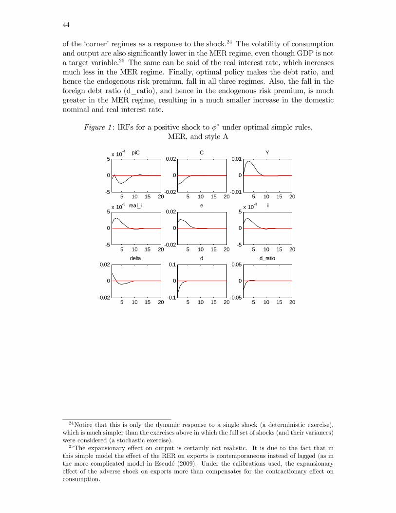
44
of the �corner�regimes as a response to the shock.24 The volatility of consumptionand output are also signi�cantly lower in the MER regime, even though GDP is nota target variable.25 The same can be said of the real interest rate, which increasesmuch less in the MER regime. Finally, optimal policy makes the debt ratio, andhence the endogenous risk premium, fall in all three regimes. Also, the fall in theforeign debt ratio (d_ratio), and hence in the endogenous risk premium, is muchgreater in the MER regime, resulting in a much smaller increase in the domesticnominal and real interest rate.
Figure 1 : lRFs for a positive shock to �� under optimal simple rules,MER, and style A
5 10 15 205
0
5x 10⁴ piC
5 10 15 200.02
0
0.02C
5 10 15 200.01
0
0.01Y
5 10 15 205
0
5x 10³ real_ii
5 10 15 200.02
0
0.02e
5 10 15 205
0
5x 10³ ii
5 10 15 200.02
0
0.02delta
5 10 15 200.1
0
0.1d
5 10 15 200.05
0
0.05d_ratio
24Notice that this is only the dynamic response to a single shock (a deterministic exercise),which is much simpler than the exercises above in which the full set of shocks (and their variances)were considered (a stochastic exercise).25The expansionary e¤ect on output is certainly not realistic. It is due to the fact that in
this simple model the e¤ect of the RER on exports is contemporaneous instead of lagged (as inthe more complicated model in Escudé (2009). Under the calibrations used, the expansionarye¤ect of the adverse shock on exports more than compensates for the contractionary e¤ect onconsumption.
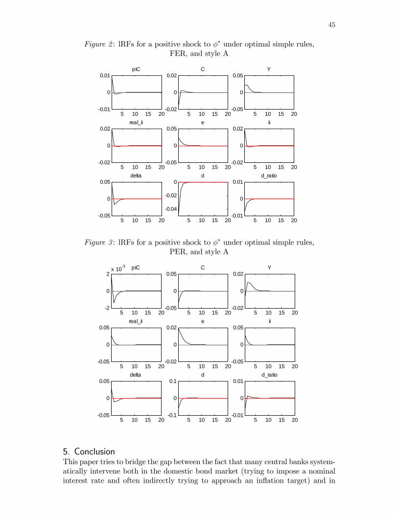
45
Figure 2 : lRFs for a positive shock to �� under optimal simple rules,FER, and style A
5 10 15 200.01
0
0.01piC
5 10 15 200.02
0
0.02C
5 10 15 200.05
0
0.05Y
5 10 15 200.02
0
0.02real_ii
5 10 15 200.05
0
0.05e
5 10 15 200.02
0
0.02ii
5 10 15 200.05
0
0.05delta
5 10 15 20
0.04
0.02
0d
5 10 15 200.01
0
0.01d_ratio
Figure 3 : lRFs for a positive shock to �� under optimal simple rules,PER, and style A
5 10 15 202
0
2x 10³ piC
5 10 15 200.05
0
0.05C
5 10 15 200.02
0
0.02Y
5 10 15 200.05
0
0.05real_ii
5 10 15 200.02
0
0.02e
5 10 15 200.05
0
0.05ii
5 10 15 200.05
0
0.05delta
5 10 15 200.1
0
0.1d
5 10 15 200.01
0
0.01d_ratio
5. ConclusionThis paper tries to bridge the gap between the fact that many central banks system-atically intervene both in the domestic bond market (trying to impose a nominalinterest rate and often indirectly trying to approach an in�ation target) and in
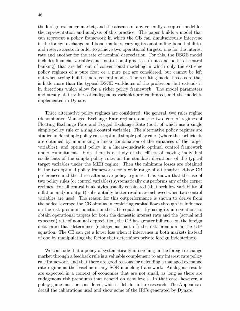
46
the foreign exchange market, and the absence of any generally accepted model forthe representation and analysis of this practice. The paper builds a model thatcan represent a policy framework in which the CB can simultaneously intervenein the foreign exchange and bond markets, varying its outstanding bond liabilitiesand reserve assets in order to achieve two operational targets: one for the interestrate and another for the rate of nominal depreciation. For this, the DSGE modelincludes �nancial variables and institutional practices (�nuts and bolts�of centralbanking) that are left out of conventional modeling in which only the extremepolicy regimes of a pure �oat or a pure peg are considered, but cannot be leftout when trying build a more general model. The resulting model has a core thatis little more than the typical DSGE workhorse of the profession, but extends itin directions which allow for a richer policy framework. The model parametersand steady state values of endogenous variables are calibrated, and the model isimplemented in Dynare.
Three alternative policy regimes are considered: the general, two rules regime(denominated Managed Exchange Rate regime), and the two �corner�regimes ofFloating Exchange Rate and Pegged Exchange Rate (both of which use a singlesimple policy rule or a single control variable). The alternative policy regimes arestudied under simple policy rules, optimal simple policy rules (where the coe¢ cientsare obtained by minimizing a linear combination of the variances of the targetvariables), and optimal policy in a linear-quadratic optimal control frameworkunder commitment. First there is a study of the e¤ects of moving individualcoe¢ cients of the simple policy rules on the standard deviations of the typicaltarget variables under the MER regime. Then the minimum losses are obtainedin the two optimal policy frameworks for a wide range of alternative ad-hoc CBpreferences and the three alternative policy regimes. It is shown that the use oftwo policy rules (or control variables) systematically outperforms any of the cornerregimes. For all central bank styles usually considered (that seek low variability ofin�ation and/or output) substantially better results are achieved when two controlvariables are used. The reason for this outperformance is shown to derive fromthe added leverage the CB obtains in exploiting capital �ows through its in�uenceon the risk premium function in the UIP equation. By using its interventions toobtain operational targets for both the domestic interest rate and the (actual andexpected) rate of nominal depreciation, the CB has greater in�uence on the foreigndebt ratio that determines (endogenous part of) the risk premium in the UIPequation. The CB can get a lower loss when it intervenes in both markets insteadof one by manipulating the factor that determines private foreign indebtedness.
We conclude that a policy of systematically intervening in the foreign exchangemarket through a feedback rule is a valuable complement to any interest rate policyrule framework, and that there are good reasons for defending a managed exchangerate regime as the baseline in any SOE modeling framework. Analogous resultsare expected in a context of economies that are not small, as long as there areendogenous risk premiums that depend on debt levels. In that case, however, apolicy game must be considered, which is left for future research. The Appendixesdetail the calibrations used and show some of the IRFs generated by Dynare.
47
ReferencesAguirre, Horacio, and Nicolás Grosman, �A note on managed �oating in a smallmacroeconomic model�, Asociación Argentina de Economía Política, XLV ReuniónAnual, November 2010.Adolfson, M., Stefan Laséen, Jesper Lindé, and Mattias Villani, �Evaluating
an Estimated New Keynesian Small Open Economy Model�, paper presented atthe joint IMF-ECB-Federal Reserve conference �DSGE Modeling at PolicymakingInstitutions: Progress & Prospects�, Washington D.C., December 2005.Agénor, Pierre-Richard, �Capital market imperfections and the macroeconomic
dynamics of small indebted economies�, Princeton Studies in International Finance,June 1997.Amato, J. D. and T. Laubach, �Estimation and control of an optimization-based
model with sticky prices and wages�, Journal of Economic Dynamics & Control 27(2003) 1181-1215.Bhandari, Jagdeep S., Nadeem Ul Haque, and Stephen J. Turnovsky, �Growth,
External Debt, and Sovereign Risk in a Small Open Economy�, International Mon-etary Fund Sta¤ Papers, 37, June 1990.Bo�nger, Peter, and Timo Wollmershaüser, �Managed Floating: understanding
the new international order�, CEPR Discussion Paper N� 3064, Nov. 2001.Calvo, Guillermo, �Staggered Prices in a Utility-Maximizing Framework�, Jour-
nal of Monetary Economics, 12 (1983), No. 3 (September):983-998.Caruana, Jaime, �Why central bank balance sheets matter�, Keynote address
at the Bank of Thailand-BIS conference on "Central bank balance sheets in Asiaand the Paci�c: the policy challeges ahead", December 2011.Christiano, Lawrence J., Martin Eichenbaum, Charles Evans, �Nominal rigidi-
ties and the dynamic e¤ects of a shock to monetary policy�, NBER Working Paper8403, July 2001.Clarida, Richard, Jordi Galí, and Mark Gertler, �The Science of Monetary Pol-
icy: A New Keynesian Perspective�, Journal of Economic Literature, Vol. XXXVII(December 1989), pp. 1661-1707.De Paoli, Bianca, �Monetary Policy and Welfare in a Small Open Economy�,
Centre for Economic Performance Discussion paper No. 639, 2006.Devereux, Michael B. and Phillip Lane, �Exchange rates and monetary policy
in emerging market economies�, unpublished manuscript, April 2003.Devereux, Michael B. and Charles Engel, �Expenditure Switching vs. Real
Exchange Rate Stabilization: Competing Objectives for Exchange Rate Policy�,unpublished manuscript, April 2004.Escudé, Guillermo J., �ARGEMmy: an intermediate DSGE model calibrated/
estimated for Argentina�, unpublished paper presented to the XIII meeting of theResearchers�Network, CEMLA , México, November 5-7, 2008.Escudé, Guillermo J. �ARGEM: a DSGEmodel with banks and monetary policy
regimes with two feedback rules, calibrated for Argentina�, Working Paper #21,Central Bank of Argentina, June 2007.Escudé, Guillermo J. �Alternative monetary regimes in a DSGE model of a
small open economy with sticky prices and wages�, Working Paper #12, CentralBank of Argentina, July 2006.
48
Gali, Jordi and Tommaso Monacelli. �Monetary Policy And Exchange RateVolatility In A Small Open Economy�, Review of Economic Studies, 2005.Giannoni, Marc P., and Michael Woodford, �Optimal Interest-Rate Rules: I.
General Theory�, NBER Working Paper No. 9419, december 2002.IMF, Regional Economic Outlook�Western Hemisphere: Watching Out for
Overheating, 2011.Juillard, M. (1996): �Dynare: a program for the resolution and simulation of
dynamic models with forward variables through the use of a relaxation algorithm�,CEPREMAP working papers 9602, CEPREMAP.Kim, Soyoung, �Monetary policy, foreign exchange intervention, and the ex-
change rate in a unifying framework�, Journal of International Economics 60 (2003)355-386.Klein, Paul, "Using the generalized Schur form to solve a multivariate linear
rational expectations model", Journal of Economic Dynamics & Control, 24 (2000)1405-1423.Kollman, Robert, �The exchange rate in a dynamic-optimizing business cycle
model with nominal rigidities: a quantitative investigation�, Journal of Interna-tional Economics 55 (2001) 243-262.Kydland, F. and E. Prescott �Rules rather than discretion: the inconsistency
of optimal plans�, Journal of Political Economy 87, 1977, 473-492.Levine, Paul, Peter McAdam and Joseph Pearlman, �Quantifying and sustain-
ing welfare gains from monetary commitment�, ECB Working Paper Series, No.709, January 2007.Mancini Gri¤oli, Tommaso, �An introduction to the solution & estimation of
DSGE models�, Dynare website, 2007McCallum, Bennett T., �A reconsideration of the uncovered interest parity re-
lationship�, Journal of Monetary Economics 33 (1994) 105-132.McCallum, Bennett T. and Edward Nelson, �Monetary policy for an open econ-
omy: an alternative framework with optimizing agents and sticky prices�, OxfordReview of Economic Policy, Vol. 16, No. 4, 2000.Montiel, Peter J., �Determinants of the Long-Run Equilibrium Real Exchange
Rate: An Analytical Treatment�. Chapter in Hinkle and Montiel (1999).Julio H. G. Olivera, �On Passive Money�, The Journal of Political Economy,
Vol. 78, No. 4, Jul.-Aug., 1970.Rotemberg, Julio J. and Michael Woodford, �Interest Rate Rules in an Esti-
mated Sticky Price Model�, in John B. Taylor (1999).Sarno, Lucio and Mark P. Taylor, �O¢ cial Intervention in the Foreign Exchange
Market: is it e¤ective and, if so, how does it work?�, Journal of Economic Litera-ture, Vol. XXXIX (September 2001), pp. 839-868.Schmitt-Grohé, S., Uribe, M., 2004 �Optimal �scal and monetary policy under
sticky prices�, Journal of Economic Theory, 114, 198-230.Schmitt-Grohé, S., Uribe, M., 2003. �Closing small open economy models�.
Journal of International Economics 61, 163-185.Schmitt-Grohé, S., Uribe, M., 2007, �Optimal In�ation Stabilization in a medium-
scale macroeconomic model�. In Mishkin, Frederic S., and Klaus-Schmidt-Hebbel(editors), �Monetary Policy under In�ation Targeting�, Banco Central de Chile.Smets Frank and RafWouters, �Openness, imperfect exchange rate pass-through,
49
and monetary policy�, European Central Bank Working Paper No. 128, March2002.Svensson, Lars E.O., �Open-economy in�ation targeting�, NBERWorking Paper
6545, May 1998.Svensson, Lars E.O�and Michael Woodford, �Optimal Policy with Partial In-
formation in a Forward-Looking Model: Certainty-Equivalence Redux�, June 2002.Taylor, John B. (editor),Monetary Policy Rules, NBER Business Cycles Series,
Volume 31, The University of Chicago Press 1999.Turnovsky, Stephen J., Methods of Macroeconomic Dynamics, second edition,
MIT Press, 2000.Walsh, Carl, Monetary Theory and Policy, second edition, The MIT Press,
2003.Williamson, John (2007), �Do development considerations matter for exchange
rate policy?�. InCurrent Account and External Financing, edited by Cowan, Kevin,Sebastián Edwards and Rodrigo O. Valdés, Central Bank of Chile.Wollmerhaüser, Timo, A Theory of Managed Floating, Inaugural-dissertation,
Würzburg, 2003.Woodford, Michael, Interest and Prices, 2003.Yun, T., �Nominal Price Rigidity, Money Supply Endogeneity, and Business
Cycles�, Journal of Monetary Economics, 37 (2) April 1996:345-370.

50
Appendix 1. Calibration of parameters and derivation of the correspond-ing non-stochastic steady stateIn this Appendix I obtain the calibrated values for the model�s parameters andthe corresponding non-stochastic steady state (NSS) values of the model variables.There are always many ways of doing this. I calibrate some of the parameters,some ratios and some NSS values of endogenous variables, and obtain the restsequentially from the static nonlinear equations so that a computer code can followthe same steps if one changes some of the calibrated values or estimates some ofthem from the data.
A.1.1. Calibration of the components of the external terms of tradeThe terms of trade is a particularly important variable for any SOE. Hence, I madea preliminary investigation of the data pertaining to Argentina. To confront (77)with the data, notice that the �rst two of these equations can be written in termsof the (logs of) price indexes:
� logP �Xt = ���X� logP �Xt�1 +
�1� ���X
�log ��X + ���X
�logP �Xt�1 � logP �Nt�1
�+��
�X"�
�X
t ;
� logP �Nt = ���� logP �Nt�1 + (1� ���) log ��N + ���
�logP �Xt�1 � logP �Nt�1
�+��
�"�
�
t :
A quick estimation for cointegration of Argentina�s trade price indexes during1993Q3-2009Q2 gave the results in the table below (the notation should be ob-vious). Although empirically I was not able to impose a coe¢ cient of negativeone for the second coe¢ cient in the cointegrating relation, I did impose it in thecalibration to be consistent with the de�nition of the terms of trade. I also ignoredthe small deterministic trend in the cointegrating relation, the two time dummies(�rst and fourth quarters of 2008) that made the residuals normal, homoscedasticand devoid of serial correlation, as well as the non-signi�cant coe¢ cients. Hence,I use the following speci�cation in the model:
� logP �Xt = 0:41� logP �Xt�1 + (1� 0:41) log ��X � 0:25�logP �Xt�1 � logP �Nt�1
�+0:0424"�
��
t ;
� logP �Nt = 0:20� logP �Nt�1 + (1� 0:20) log ��N + 0:18�logP �Xt�1 � logP �Nt�1
�+0:18� logP �Xt�1 + 0:0295"
��
t ;
where, using the notation in (77), ��� = 1, and ���XN = 0:18 is added for the e¤ect
of � logP �Xt�1 on � logP�Nt (which did not appear in the original speci�cation).
Hence, the �nal speci�cation of the XTT block (77) is:
��Xt =���Xt�1
�0:41 ���X
�1�0:41 �p�t�1
��0:25exp
�0:0424"�
��
t
�;
��t =���t�1
�0:20(��)1�0:20
�p�t�1
�0:18 ���Xt
�0:18exp
�0:0295"�
�
t
�;
p�t = p�t�1��Xt��t:
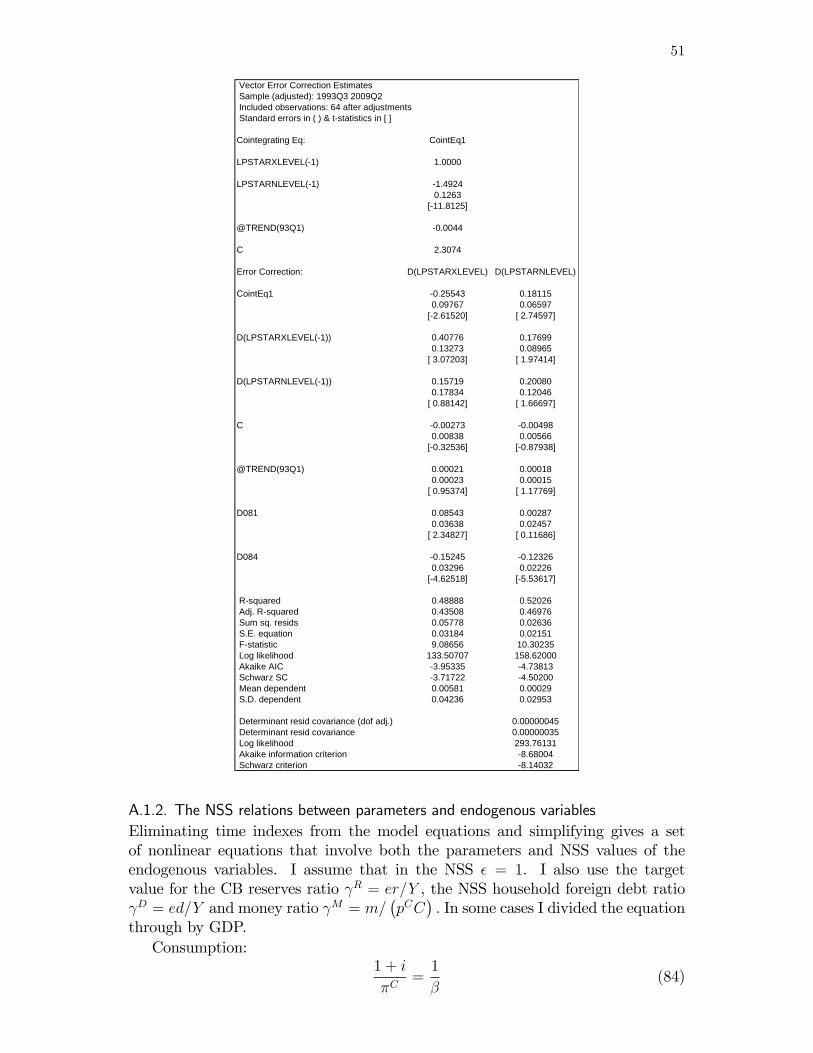
51
Vector Error Correction Estimates Sample (adjusted): 1993Q3 2009Q2 Included observations: 64 after adjustments Standard errors in ( ) & tstatistics in [ ]
Cointegrating Eq: CointEq1
LPSTARXLEVEL(1) 1.0000
LPSTARNLEVEL(1) 1.49240.1263
[11.8125]
@TREND(93Q1) 0.0044
C 2.3074
Error Correction: D(LPSTARXLEVEL) D(LPSTARNLEVEL)
CointEq1 0.25543 0.181150.09767 0.06597
[2.61520] [ 2.74597]
D(LPSTARXLEVEL(1)) 0.40776 0.176990.13273 0.08965
[ 3.07203] [ 1.97414]
D(LPSTARNLEVEL(1)) 0.15719 0.200800.17834 0.12046
[ 0.88142] [ 1.66697]
C 0.00273 0.004980.00838 0.00566
[0.32536] [0.87938]
@TREND(93Q1) 0.00021 0.000180.00023 0.00015
[ 0.95374] [ 1.17769]
D081 0.08543 0.002870.03638 0.02457
[ 2.34827] [ 0.11686]
D084 0.15245 0.123260.03296 0.02226
[4.62518] [5.53617]
Rsquared 0.48888 0.52026 Adj. Rsquared 0.43508 0.46976 Sum sq. resids 0.05778 0.02636 S.E. equation 0.03184 0.02151 Fstatistic 9.08656 10.30235 Log likelihood 133.50707 158.62000 Akaike AIC 3.95335 4.73813 Schwarz SC 3.71722 4.50200 Mean dependent 0.00581 0.00029 S.D. dependent 0.04236 0.02953
Determinant resid covariance (dof adj.) 0.00000045 Determinant resid covariance 0.00000035 Log likelihood 293.76131 Akaike information criterion 8.68004 Schwarz criterion 8.14032
A.1.2. The NSS relations between parameters and endogenous variablesEliminating time indexes from the model equations and simplifying gives a setof nonlinear equations that involve both the parameters and NSS values of theendogenous variables. I assume that in the NSS � = 1. I also use the targetvalue for the CB reserves ratio R = er=Y , the NSS household foreign debt ratio D = ed=Y and money ratio M = m=
�pCC
�: In some cases I divided the equation
through by GDP.Consumption:
1 + i
�C=1
�(84)

52
Risk-adjusted uncovered interest parity:
1 + i = (1 + i�)��'D� D�� (85)
Phillips in�ation equations:
� =Q=�pCC�
C�
1� �����1 (86)
=�
� � 1mcQ=�pCC�
C�
1� ���� (87)
�
=
�1� ����11� �
� 1��1
= ep (�)�1 (88)
Dynamics of price dispersion:
� =
�1� �1� ���
��1� ����11� �
� ���1
: (89)
Exports:X = �X (ep
�)bX Y (90)
Trade Balance:
TBe
Y=1
aD
��pCt�1��C X
Y� (1� aD) e1��
C
�(91)
Current Account:
CAe
Y=
�1 + i�
��� 1� R �
�1 + i�
�����D
� D�� 1� D + TB
e
Y(92)
Balance of Payments:CA = 0 (93)
Real marginal cost:mc = w (94)
Labor market clearing:
w = �NpCC�C
'M� M�N�N (95)
Hours worked:N = Q� (96)
Domestic goods market clearing:
Q
Y= 1�
�1� bA
� XY
(97)
GDP:
1 = aD�M� M�G
(pC)1��C
pCC
Y+X
Y(98)

53
Consumption relative price:
pC =�aD + (1� aD) e1��
C� 1
1��C (99)
Money market balance:m = L (1 + i) pCC; (100)
CB balance sheet:b
Y= R � M p
CC
Y(101)
Consumption in�ation:�C = � (102)
Real Exchange Rate:��� = � (103)
External terms of trade:��X = �� (104)
Tax collection:tax = GpCC � qf
Quasi-�scal surplus:
qf = (1 + i� � 1=�) er��� ((1 + i)� 1) b
�
Interest rate feedback rule:
1 =
��C
�T
�h1(105)
Nominal depreciation feedback rule:
1 =
��C
�T
�k1 �er=Y R
�k4(106)
Exports in�ation shock1 = (p�)���� (107)
Imported in�ation shock
1 = (p�)������X
����XN: (108)
I now show one way in which the EENE values of the model�s variables and thecalibrated values of parameters can be obtained sequentially.(105) implies �C = �T , since h1 6= 0 is assumed. Inserting this in (102) yields
� = �T . Also, (107) implies that the XTT is p� = 1, and hence (108) implies that��X = 1, and (104) that �� = 1. Therefore, (103) implies � = �T . Summing up,we have:
� = � = �C = �T ; and �� = ��X = p� = 1:
Hence, (84) gives the nominal interest rate: 1+ i = �T=� and (106) yields er=Y = R, since it is assumed that k4 6= 0, which implies that the CB�s target ratio ofinternational reserves to GDP is attained in the NSS.
54
I assume � = 0:99. For illustrative purposes I use as Argentina�s NSS GDP its2010 level (at 2010 prices and in trillions of pesos): Y = 1:443. The gross exogenousrisk/liquidity premium for households and the RW gross interest rate are assumedto be �� = 1:0050:25 and 1 + i� = 1:030:25, respectively. Also, the household ratiosare D � ed=Y = 0:5, M � m=pCC = 0:095522, and Government to householdconsumption ratio is assumed to be G = 1:19.The home bias parameter (or share of domestic goods) in household consump-
tion is calibrated to aD = 0:86. The constant relative risk aversion for labor (whichis also the inverse of the elasticity of labor supply with respect to the real wage)and consumption are: �N = 0:5 and �C = 1:5, respectively. Finally, I assume thatthe elasticity of substitution between varieties of domestic goods is � = 6 and theelasticity of substitution between the bundles of domestic and imported goods is�C = 1:5. Assuming that the exogenous parameter for exports demand is bA = 0:5,
yields bX ��1� bA
��1= 2 and �X �
�bA�bAbX
= 0:5.I now focus on the NSS values of the remaining endogenous variables and pa-
rameters.
A.1.2.1 The endogenous risk premium
Using (84), (102), and (103) in the UIP equation (85) gives the household foreigndebt to GDP ratio as a function of parameters which I have already calibrated:
D � ed
Y= '�1D
�1=�
�� (1 + i�) =��
�= '�1D
�1
��� (1 + i�)
�:
However, calculating this requires the values of the exogenous parameters �1 and�2 which help de�ne the function 'D. I now seek to calibrate them in terms of themore intuitive elasticity of the risk premium function in the UIP (which plays acritical role in the present research). First, notice that the elasticity "D of �D is
"D� Dt�� �2
Dt
1� �2 Dt: (109)
�D and 'D are related to "D by (see (67) and (69)):
�D� Dt�= �1
�1 + "D(
Dt )�; (110)
'D� Dt�= �1
�1 + "D(
Dt )�2:
Hence, if the NSS values of "D and D are calibrated, (109) gives the value of �2:
�2 =1
D�1"D+ 1� : (111)
Also, using (110), (66), and (84) in (85) yields:
'D� D�=
1 + i
(1 + i�)���� 1 = 1
� (1 + i�)��� 1 = �1 (1 + "D)2 ; (112)

55
which gives the value of �1:
�1 =1
(1 + "D)2
�1
� (1 + i�)��� 1�=�1� �2 D
�2� 1
� (1 + i�)��� 1�; (113)
where the second equality is derived from (111).However, because of the critical role of the derived function 'D in the UIP
equation (71) it is perhaps more intuitive in calibrations to start with the value ofthe elasticity of 'D, which I denote as "
'D, along with
D, and derive the value of"D. It is straightforward to prove that "
'D and "D are related by:
"'D = "D2
D'D
1 + 'D= "D
2
D[1� � (1 + i�)��] ; (114)
where the second equality uses (112). Hence, using (111), (113) and (109):
�2 =1
2"'D[1� � (1 + i�)��] + D
�1 =�1� �2 D
�2� 1
� (1 + i�)��� 1�:
If, say, "'D = 2 then
�2 =1
(1� 0:99 (1:030:25) 1:0050:25) + 0:5 = 1: 994 4
�1 = (1� 1: 994 4 � 0:5)2�
1
0:99 (1:030:25) 1:0050:25� 1�= 1: 109 2� 10�8
and hence:
�D =1: 1092� 10�81� 1:9944 � 0:5 = 3:9614� 10
�6
'D =1:1092� 10�8
(1� 1:994 4 � 0:5)2= 1:4148� 10�3:
A.1.2.2 The balance of payments
Using the previous calibrations, (93) and (92) give the trade balance to GDP rationecessary to sustain net interest payments abroad:
TBe
Y=
�1 + i�
�����D � 1
� D �
�1 + i�
��� 1� R�
1:030:25
11:0050:25 (1:0000039368)� 1
�0:5�
�1:030:25
1� 1�0:13
= 0:00337476
56
Then, using (91), (90), and (99), one can obtain the RER necessary to generatethis trade surplus:
�X (ep�)bX
haD + (1� aD) e1��
Ci� (1� aD) e1��
C
= aDTBe
Y0:5e2
�0:86 + (1� 0:86) e1�1:5
�� (1� 0:86) e1�1:5 = 0:86 (0:00337476)
e = 0:595055
and hence the exports to GDP ratio and pC :
X
Y= �X (ep
�)bX = 0:5 (0:595055)2 = 0:177 045;
pC =�0:86 + (1� 0:86) (0:595055)1�1:5
� 11�1:5 = 0:921915
A.1.2.3 The transactions cost function and money demand
The elasticity of L (1 + i) (see (70)) can be shown to satisfy the following relation:
"L� M�=
1
(�3 + 1) i
�1 +
1
�2 M
�; (115)
from which we obtain:
�2 =1
M1
(�3 + 1) "Li� 1:
Also, reshu ing (70) gives:
�1 =
�1 + �2
M��3+1
�2�3
�1� 1
1 + i
�:
So using the last two expressions in (68) to eliminate �1 and �2 gives:
�M� M�=
�1 +
1
�3
��1� 1
1 + i
�i"L� M� M : (116)
Since transaction costs are dependent on the in�ation rate (through the nominalinterest rate) I cannot calibrate the three parameters �1; �2; and �3 without �rstcalibrating the in�ation rate. I assume that the target in�ation rate is �T = 1:015.Hence, the nominal interest rate is given by (84): 1+i = 1:015=0:99 = 1:0253: Next,calibrate the value of the interest elasticity of money demand to, say, "L = 1:02. Wealso have M = 0:095522. Notice that to have �2 positive, �3 must be su¢ cientlyhigh (and hence �M su¢ ciently low):26
26Although this level of transaction costs may seem unrealistically low, we really do not caremuch about transaction costs per se but only their e¤ect on money demand. To have morerealistic levels of transaction costs we would need a di¤erent transaction costs function. As longas we are confortable with the resulting interest elasticity of money demand and the assumedstock of money, we can hold on to the present function.

57
�3 >1
"Li� 1 = 1
1:02 (1:015=0:99� 1) � 1 = 37:82352941
�M <
�1 +
1
37:82352941
��1� 1
1:015=0:99
��1:015
0:99� 1�0:095522 � 1:02
= 0:00006220357:
If, say, �3 = 160, then:
�2 =1
0:09553
1
(160 + 1) 1:02�1:0150:99
� 1�� 1
= 3:32635
�1 =(1 + 3:32635 � 0:095522)160+1
3:32635 � 160
�1� 0:99
1:015
�= 9:07697� 1014:
Hence:
�M =�1
(1 + �2 M)�3
=9:07697� 1014
(1 + 3:32635 � 0:095522)160= 6:0984� 10�5
'M = �M
�1 + �3
�2 M
1 + �2 M
�= 6:0984� 10�5
�1 + 160
3:32635 � 0:0955221 + 3:32635 � 0:095522
�= 2:41374� 10�3:
Finally, using (98), the consumption to GDP ratio is:
pCC
Y=
�pC�1��C
aD�M ( M)G
h1� �X (ep�)b
Xi
=(0:921915)1�1:5
0:86 � 1:00006098 � 1:19 (1� 0:177 045) = 0:837457:
Hence, C and Q can be obtained:
C =pCC
Y
Y
pC= 0:837457 � 1:443
0:921915= 1: 310 8
Q =
�1�
�1� bA
� XY
�Y = [1� (1� 0:5) 0:177 045] 1:443 = 1: 315 26:
A.1.2.4 In�ation, price dispersion and marginal cost
(89) shows NSS price dispersion as a function of the NSS in�ation rate. It is easyto check that this function has a local minimum at � = 1, where there is pricestability and no price dispersion (� = 1). Given the above calibrations, the NSSvalue of price dispersion is:
� =1� 0:66
1� 0:66 (1:015)6
1� 0:66 (1:015)6�1
1� 0:66
! 66�1
= 1:0051:
58
Hence, (97) gives the value of hours worked:
N = Q� = 1:31526 � 1:0051 = 1:32197;
(86) gives the value of �:
� =Q=�pCC�
C�
1� �����1 =1: 315 26= (0:921915 � 1: 310 81:5)1� 0:99 � 0:66 � 1:0156�1 = 3:210508;
(88) gives the value of :
= �
�1� �
1� ����1
� 1��1
= 3:210508
�1� 0:66
1� 0:66 � 1:0156�1
� 16�1
= 3:31659;
and (87) gives the value of mc:
mc =
,0@ �
� � 1Q=�pCC�
C�
1� ����
1A= 3: 316 59
��6
6� 11: 315 26= (0:921915 � 1: 310 81:5)
1� 0:99 � 0:66 � 1:0156
�= 0:830 17:
Finally, (94) and (95) give the value of �N :
�N = mc=�pCC�
C
'MN�N�
= 0:83017��0:921915 � 1:31081:51:0024137 � 1:321970:5
�= 0:520612;
and the NSS value of period aggregate utility is:
Utility =1: 31081�1:5
1� 1:5 � 0:5206121:321971+0:5
1 + 0:5= �2:2744:
The fact that it is negative is irrelevant, since utility has only ordinal, not cardinal,signi�cance.

59
Appendix 2. Impulse Response Functions for Optimal Policies in theMER regime under CB styles A, B, and CAll shocks in the IRFs below are positive and of 1 standard deviation. Shockvariables are in logs in the nonlinear model.
A.2.1 Optimal Simple Policy RulesA.2.1.1 Central Bank style A
!� = 100; !Y = 1; !e = 1; !r = 1; !�i = 50; !�� = 50
h0 h1 h2 h3 k0 k1 k2 k3 k40:33 1:26 0:02 0:12 �0:03 �0:07 �0:08 �0:43 �0:08Response to a positive shock to domestic sector productivity: �
5 10 15 202
1
0x 103 piC
5 10 15 201
0.5
0x 103 DeltaP
5 10 15 200
0.005
0.01Y
5 10 15 200
0.005
0.01C
5 10 15 202
1
0x 103 real_ii
5 10 15 202
0
2x 10⁴ e
5 10 15 205
0
5x 104 TB
5 10 15 200
1
2x 103 X
5 10 15 204
2
0x 103 mc
5 10 15 200.01
0.005
0N
5 10 15 204
2
0x 103 ii
5 10 15 202
1
0x 103 delta
5 10 15 200
2
4x 10³ b
5 10 15 200
0.005
0.01r
5 10 15 200
0.005
0.01d
5 10 15 200
0.5
1x 10³ m
5 10 15 200
0.005
0.01Utility
5 10 15 200
0.01
0.02z_epsilon

60
Response to a positive shock to government expenditures: G
5 10 15 202
0
2x 10⁴ piC
5 10 15 202
0
2x 10⁴ DeltaP
5 10 15 200
0.02
0.04Y
5 10 15 200.01
0.005
0C
5 10 15 201
0
1x 10³ real_ii
5 10 15 205
0
5x 10³ e
5 10 15 200.01
0
0.01TB
5 10 15 200
2
4x 103 X
5 10 15 205
0
5x 10³ mc
5 10 15 200
0.02
0.04N
5 10 15 201
0
1x 10³ ii
5 10 15 205
0
5x 10³ delta
5 10 15 200.02
0
0.02b
5 10 15 200.05
0
0.05r
5 10 15 200
0.02
0.04d
5 10 15 201
0.5
0x 103 m
5 10 15 200.04
0.02
0Utility
5 10 15 200
0.02
0.04z_G
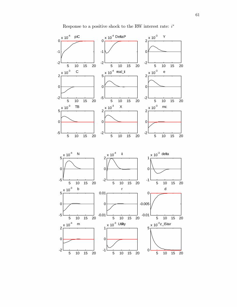
61
Response to a positive shock to the RW interest rate: i�
5 10 15 202
1
0x 104 piC
5 10 15 202
1
0x 104 DeltaP
5 10 15 202
0
2x 10³ Y
5 10 15 202
0
2x 10³ C
5 10 15 205
0
5x 10⁴ real_ii
5 10 15 202
0
2x 10³ e
5 10 15 205
0
5x 103 TB
5 10 15 202
0
2x 103 X
5 10 15 202
0
2x 10³ mc
5 10 15 205
0
5x 10⁴ N
5 10 15 202
0
2x 10⁴ ii
5 10 15 201
0
1x 10³ delta
5 10 15 205
0
5x 10³ b
5 10 15 200.01
0
0.01r
5 10 15 200.01
0.005
0d
5 10 15 202
0
2x 10⁴ m
5 10 15 201
0
1x 10³ Utility
5 10 15 200
5x 10³z_iStar

62
Response to a positive shock to the SOE�s exogenous risk/liquidity premium: ��
5 10 15 205
0
5x 10⁴ piC
5 10 15 201
0
1x 10³ DeltaP
5 10 15 200.01
0
0.01Y
5 10 15 200.02
0
0.02C
5 10 15 205
0
5x 10³ real_ii
5 10 15 200.02
0
0.02e
5 10 15 200.05
0
0.05TB
5 10 15 200.02
0
0.02X
5 10 15 200.01
0
0.01mc
5 10 15 205
0
5x 10³ N
5 10 15 205
0
5x 10³ ii
5 10 15 200.02
0
0.02delta
5 10 15 200.05
0
0.05b
5 10 15 200.1
0
0.1r
5 10 15 200.1
0
0.1d
5 10 15 201
0
1x 10³ m
5 10 15 200.01
0
0.01Utility
5 10 15 200
0.05
0.1z_phiStar

63
Response to a positive shock to imports in�ation: ��
5 10 15 205
0
5x 10³ piC
5 10 15 205
0
5x 10⁴ DeltaP
5 10 15 200.01
0
0.01Y
5 10 15 200.01
0
0.01C
5 10 15 200.01
0
0.01real_ii
5 10 15 200.02
0
0.02e
5 10 15 200.01
0
0.01TB
5 10 15 200.01
0
0.01X
5 10 15 200.01
0
0.01mc
5 10 15 200.01
0
0.01N
5 10 15 200.01
0
0.01ii
5 10 15 200.02
0
0.02delta
5 10 15 200.01
0
0.01b
5 10 15 200.02
0
0.02r
5 10 15 200.02
0
0.02d
5 10 15 202
0
2x 10³ m
5 10 15 205
0
5x 10³ Utility
5 10 15 200.05
0
0.05z_piStar

64
Response to a positive shock to exports in�ation: ��X
5 10 15 205
0
5x 10³ piC
5 10 15 202
0
2x 10³ DeltaP
5 10 15 200.05
0
0.05Y
5 10 15 200.02
0
0.02C
5 10 15 205
0
5x 10³ real_ii
5 10 15 200.02
0
0.02e
5 10 15 200.05
0
0.05TB
5 10 15 200.02
0
0.02X
5 10 15 200.02
0
0.02mc
5 10 15 200.02
0
0.02N
5 10 15 205
0
5x 10³ ii
5 10 15 200.02
0
0.02delta
5 10 15 200.1
0
0.1b
5 10 15 200.1
0
0.1r
5 10 15 200.1
0
0.1d
5 10 15 201
0
1x 10³ m
5 10 15 200.01
0
0.01Utility
5 10 15 200.01
0
0.01z_piStar

65
A.2.1.2 Central Bank style B
!� = 1; !Y = 100; !e = 1; !r = 1; !�i = 50; !�� = 50
h0 h1 h2 h3 k0 k1 k2 k3 k41:86 �1:01 4:34 �0:21 3:08 �3:92 �2:28 1:18 0:40Response to a positive shock to domestic sector productivity: �
5 10 15 205
0
5x 10³ piC
5 10 15 205
0
5x 10³ DeltaP
5 10 15 200
0.5
1x 10³ Y
5 10 15 201
0
1x 10³ C
5 10 15 205
0
5x 10⁴ real_ii
5 10 15 201
0
1x 10³ e
5 10 15 202
0
2x 103 TB
5 10 15 201
0
1x 103 X
5 10 15 200.02
0
0.02mc
5 10 15 200.02
0
0.02N
5 10 15 200
5x 10³ ii
5 10 15 200
5x 10³ delta
5 10 15 200
5x 10³ b
5 10 15 200
0.005
0.01r
5 10 15 202
0
2x 10³ d
5 10 15 201
0.5
0x 103 m
5 10 15 200.01
0
0.01Utility
5 10 15 200
0.01
0.02z_epsilon
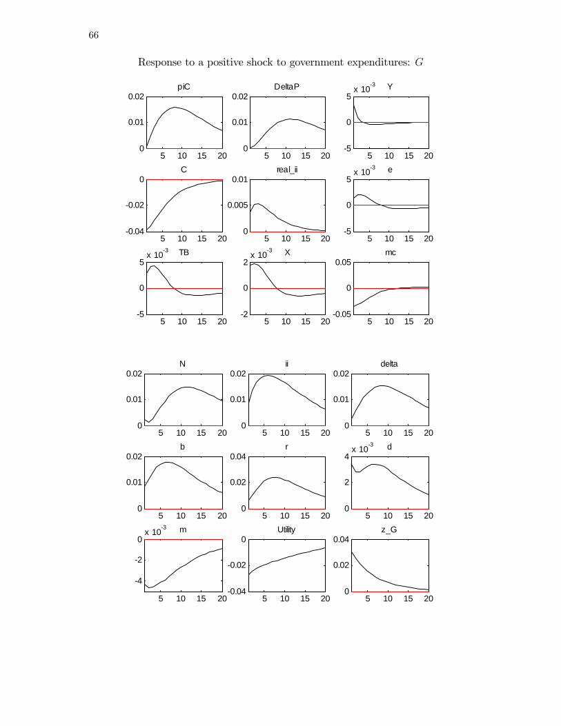
66
Response to a positive shock to government expenditures: G
5 10 15 200
0.01
0.02piC
5 10 15 200
0.01
0.02DeltaP
5 10 15 205
0
5x 10³ Y
5 10 15 200.04
0.02
0C
5 10 15 200
0.005
0.01real_ii
5 10 15 205
0
5x 10³ e
5 10 15 205
0
5x 103 TB
5 10 15 202
0
2x 103 X
5 10 15 200.05
0
0.05mc
5 10 15 200
0.01
0.02N
5 10 15 200
0.01
0.02ii
5 10 15 200
0.01
0.02delta
5 10 15 200
0.01
0.02b
5 10 15 200
0.02
0.04r
5 10 15 200
2
4x 10³ d
5 10 15 20
4
2
0x 103 m
5 10 15 200.04
0.02
0Utility
5 10 15 200
0.02
0.04z_G

67
Response to a positive shock to the RW interest rate: i�
5 10 15 202
0
2x 10³ piC
5 10 15 201
0
1x 10³ DeltaP
5 10 15 201
0
1x 10³ Y
5 10 15 202
0
2x 10³ C
5 10 15 205
0
5x 10⁴ real_ii
5 10 15 202
0
2x 10³ e
5 10 15 205
0
5x 103 TB
5 10 15 202
0
2x 103 X
5 10 15 205
0
5x 10³ mc
5 10 15 202
0
2x 10³ N
5 10 15 201
0
1x 10³ ii
5 10 15 201
0
1x 10³ delta
5 10 15 205
0
5x 10³ b
5 10 15 200.01
0
0.01r
5 10 15 200.01
0.005
0d
5 10 15 201
0.5
0x 104 m
5 10 15 201
0
1x 10³ Utility
5 10 15 200
5x 10³z_iStar

68
Response to a positive shock to the SOE�s exogenous risk/liquidity premium: ��
5 10 15 200.02
0.01
0piC
5 10 15 200.01
0.005
0DeltaP
5 10 15 200.01
0
0.01Y
5 10 15 200.02
0
0.02C
5 10 15 205
0
5x 10³ real_ii
5 10 15 200.02
0
0.02e
5 10 15 200.05
0
0.05TB
5 10 15 200.01
0
0.01X
5 10 15 200.02
0.01
0mc
5 10 15 200.02
0.01
0N
5 10 15 200.01
0.005
0ii
5 10 15 200.02
0.01
0delta
5 10 15 200.05
0
0.05b
5 10 15 200.1
0
0.1r
5 10 15 200.1
0
0.1d
5 10 15 205
0
5x 10⁴ m
5 10 15 205
0
5x 10³ Utility
5 10 15 200
0.05
0.1z_phiStar

69
Response to a positive shock to imports in�ation: ��
5 10 15 200
0.005
0.01piC
5 10 15 200
1
2x 10³ DeltaP
5 10 15 205
0
5x 10³ Y
5 10 15 205
0
5x 10³ C
5 10 15 205
0
5x 10³ real_ii
5 10 15 200.02
0
0.02e
5 10 15 200.01
0
0.01TB
5 10 15 205
0
5x 103 X
5 10 15 200
0.005
0.01mc
5 10 15 200
0.005
0.01N
5 10 15 200
2
4x 10³ ii
5 10 15 200.01
0
0.01delta
5 10 15 200.01
0
0.01b
5 10 15 200.02
0
0.02r
5 10 15 200.02
0
0.02d
5 10 15 201
0
1x 10³ m
5 10 15 204
2
0x 103 Utility
5 10 15 200.05
0
0.05z_piStar
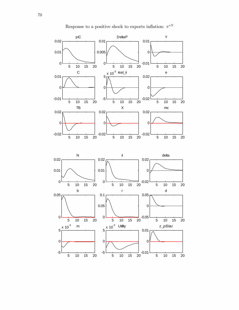
70
Response to a positive shock to exports in�ation: ��X
5 10 15 200
0.01
0.02piC
5 10 15 200
0.005
0.01DeltaP
5 10 15 200.01
0
0.01Y
5 10 15 200.01
0
0.01C
5 10 15 205
0
5x 10³ real_ii
5 10 15 200.02
0
0.02e
5 10 15 200.02
0
0.02TB
5 10 15 200.02
0
0.02X
5 10 15 200.02
0
0.02mc
5 10 15 200
0.01
0.02N
5 10 15 200
0.01
0.02ii
5 10 15 200.02
0
0.02delta
5 10 15 200
0.05b
5 10 15 200
0.05
0.1r
5 10 15 200.05
0
0.05d
5 10 15 205
0
5x 10³ m
5 10 15 205
0
5x 10³ Utility
5 10 15 200.01
0
0.01z_piStar
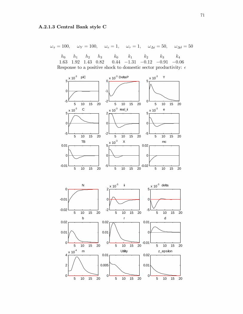
71
A.2.1.3 Central Bank style C
!� = 100; !Y = 100; !e = 1; !r = 1; !�i = 50; !�� = 50
h0 h1 h2 h3 k0 k1 k2 k3 k41:63 1:92 1:43 0:82 0:44 �1:31 �0:12 �0:91 �0:06Response to a positive shock to domestic sector productivity: �
5 10 15 205
0
5x 10³ piC
5 10 15 202
1
0x 103 DeltaP
5 10 15 200
5x 10³ Y
5 10 15 205
0
5x 10³ C
5 10 15 202
0
2x 10³ real_ii
5 10 15 205
0
5x 10³ e
5 10 15 200.01
0
0.01TB
5 10 15 205
0
5x 103 X
5 10 15 200.02
0
0.02mc
5 10 15 200.02
0.01
0N
5 10 15 202
0
2x 10³ ii
5 10 15 205
0
5x 10³ delta
5 10 15 200
0.01
0.02b
5 10 15 200
0.01
0.02r
5 10 15 200.01
0
0.01d
5 10 15 200
2
4x 10⁴ m
5 10 15 200
0.005
0.01Utility
5 10 15 200
0.01
0.02z_epsilon

72
Response to a positive shock to government expenditures: G
5 10 15 200.02
0.01
0piC
5 10 15 200.01
0.005
0DeltaP
5 10 15 200
0.01
0.02Y
5 10 15 20
0.04
0.02
0C
5 10 15 200.02
0
0.02real_ii
5 10 15 200.02
0
0.02e
5 10 15 200.05
0
0.05TB
5 10 15 200.02
0
0.02X
5 10 15 200.05
0
0.05mc
5 10 15 200
5x 10³ N
5 10 15 205
0
5x 10³ ii
5 10 15 200.02
0
0.02delta
5 10 15 200
0.05
0.1b
5 10 15 200
0.05
0.1r
5 10 15 200
0.02
0.04d
5 10 15 205
0
5x 10³ m
5 10 15 200.04
0.02
0Utility
5 10 15 200
0.02
0.04z_G

73
Response to a positive shock to the RW interest rate: i�
5 10 15 202
1
0x 103 piC
5 10 15 201
0.5
0x 103 DeltaP
5 10 15 205
0
5x 10⁴ Y
5 10 15 205
0
5x 10³ C
5 10 15 201
0
1x 10³ real_ii
5 10 15 200
1
2x 10³ e
5 10 15 200
2
4x 103 TB
5 10 15 200
1
2x 103 X
5 10 15 204
2
0x 103 mc
5 10 15 202
1
0x 103 N
5 10 15 201
0
1x 10³ ii
5 10 15 202
0
2x 10³ delta
5 10 15 205
0
5x 10³ b
5 10 15 200.01
0
0.01r
5 10 15 200.01
0.005
0d
5 10 15 202
0
2x 10⁴ m
5 10 15 201
0
1x 10³ Utility
5 10 15 200
5x 10³z_iStar

74
Response to a positive shock to the SOE�s exogenous risk/liquidity premium: ��
5 10 15 200.01
0
0.01piC
5 10 15 204
2
0x 103 DeltaP
5 10 15 205
0
5x 10³ Y
5 10 15 200.05
0
0.05C
5 10 15 200.01
0
0.01real_ii
5 10 15 200.02
0
0.02e
5 10 15 200.05
0
0.05TB
5 10 15 200.02
0
0.02X
5 10 15 200.05
0
0.05mc
5 10 15 200.02
0
0.02N
5 10 15 200.01
0
0.01ii
5 10 15 200.02
0
0.02delta
5 10 15 200.05
0
0.05b
5 10 15 200.1
0
0.1r
5 10 15 200.1
0
0.1d
5 10 15 202
0
2x 10³ m
5 10 15 200.01
0
0.01Utility
5 10 15 200
0.05
0.1z_phiStar
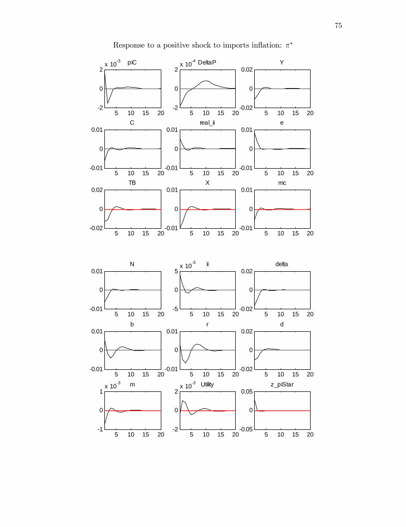
75
Response to a positive shock to imports in�ation: ��
5 10 15 202
0
2x 10³ piC
5 10 15 202
0
2x 10⁴ DeltaP
5 10 15 200.02
0
0.02Y
5 10 15 200.01
0
0.01C
5 10 15 200.01
0
0.01real_ii
5 10 15 200.01
0
0.01e
5 10 15 200.02
0
0.02TB
5 10 15 200.01
0
0.01X
5 10 15 200.01
0
0.01mc
5 10 15 200.01
0
0.01N
5 10 15 205
0
5x 10³ ii
5 10 15 200.02
0
0.02delta
5 10 15 200.01
0
0.01b
5 10 15 200.01
0
0.01r
5 10 15 200.02
0
0.02d
5 10 15 201
0
1x 10³ m
5 10 15 202
0
2x 10³ Utility
5 10 15 200.05
0
0.05z_piStar
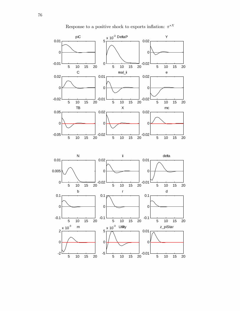
76
Response to a positive shock to exports in�ation: ��X
5 10 15 200.01
0
0.01piC
5 10 15 200
5x 10³ DeltaP
5 10 15 200.02
0
0.02Y
5 10 15 200.02
0
0.02C
5 10 15 200.01
0
0.01real_ii
5 10 15 200.02
0
0.02e
5 10 15 200.05
0
0.05TB
5 10 15 200.02
0
0.02X
5 10 15 200.02
0
0.02mc
5 10 15 200
0.005
0.01N
5 10 15 200.02
0
0.02ii
5 10 15 200.01
0
0.01delta
5 10 15 200.1
0
0.1b
5 10 15 200.1
0
0.1r
5 10 15 200.1
0
0.1d
5 10 15 202
0
2x 10³ m
5 10 15 205
0
5x 10³ Utility
5 10 15 200.01
0
0.01z_piStar
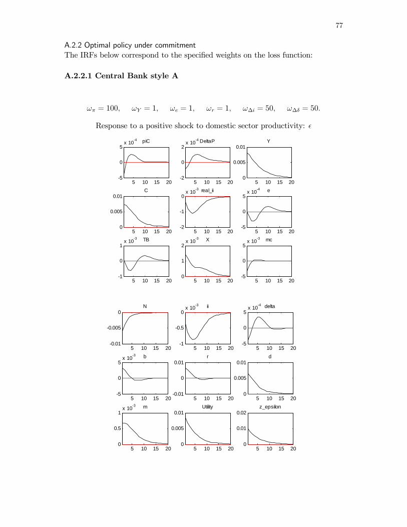
77
A.2.2 Optimal policy under commitmentThe IRFs below correspond to the speci�ed weights on the loss function:
A.2.2.1 Central Bank style A
!� = 100; !Y = 1; !e = 1; !r = 1; !�i = 50; !�� = 50:
Response to a positive shock to domestic sector productivity: �
5 10 15 205
0
5x 10⁴ piC
5 10 15 202
0
2x 10⁴ DeltaP
5 10 15 200
0.005
0.01Y
5 10 15 200
0.005
0.01C
5 10 15 202
1
0x 103 real_ii
5 10 15 205
0
5x 10⁴ e
5 10 15 201
0
1x 103 TB
5 10 15 200
1
2x 103 X
5 10 15 205
0
5x 10³ mc
5 10 15 200.01
0.005
0N
5 10 15 201
0.5
0x 103 ii
5 10 15 205
0
5x 10⁴ delta
5 10 15 205
0
5x 10³ b
5 10 15 200.01
0
0.01r
5 10 15 200
0.005
0.01d
5 10 15 200
0.5
1x 10³ m
5 10 15 200
0.005
0.01Utility
5 10 15 200
0.01
0.02z_epsilon
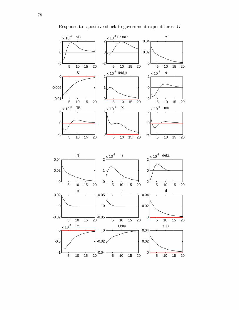
78
Response to a positive shock to government expenditures: G
5 10 15 205
0
5x 10⁴ piC
5 10 15 202
0
2x 10⁴ DeltaP
5 10 15 200
0.02
0.04Y
5 10 15 200.01
0.005
0C
5 10 15 200
1
2x 10³ real_ii
5 10 15 202
0
2x 10³ e
5 10 15 205
0
5x 103 TB
5 10 15 200
5x 103 X
5 10 15 202
0
2x 10³ mc
5 10 15 200
0.02
0.04N
5 10 15 200
1
2x 10³ ii
5 10 15 202
0
2x 10³ delta
5 10 15 200.02
0
0.02b
5 10 15 200.05
0
0.05r
5 10 15 200
0.02
0.04d
5 10 15 201
0.5
0x 103 m
5 10 15 200.04
0.02
0Utility
5 10 15 200
0.02
0.04z_G

79
Response to a positive shock to the RW interest rate: i�
5 10 15 205
0
5x 10⁴ piC
5 10 15 202
0
2x 10⁴ DeltaP
5 10 15 202
0
2x 10³ Y
5 10 15 202
0
2x 10³ C
5 10 15 205
0
5x 10⁴ real_ii
5 10 15 200
1
2x 10³ e
5 10 15 200
2
4x 103 TB
5 10 15 200
1
2x 103 X
5 10 15 202
0
2x 10³ mc
5 10 15 201
0
1x 10³ N
5 10 15 205
0
5x 10⁴ ii
5 10 15 201
0
1x 10³ delta
5 10 15 205
0
5x 10³ b
5 10 15 200.01
0
0.01r
5 10 15 200.01
0.005
0d
5 10 15 202
0
2x 10⁴ m
5 10 15 201
0.5
0x 103 Utility
5 10 15 200
5x 10³z_iStar

80
Response to a positive shock to the SOE�s exogenous risk/liquidity premium: ��
5 10 15 202
0
2x 10³ piC
5 10 15 201
0
1x 10³ DeltaP
5 10 15 200.01
0
0.01Y
5 10 15 200.02
0
0.02C
5 10 15 205
0
5x 10³ real_ii
5 10 15 200.01
0
0.01e
5 10 15 200.02
0
0.02TB
5 10 15 200.01
0
0.01X
5 10 15 200.02
0
0.02mc
5 10 15 200.01
0
0.01N
5 10 15 205
0
5x 10³ ii
5 10 15 200.01
0
0.01delta
5 10 15 200.05
0
0.05b
5 10 15 200.1
0
0.1r
5 10 15 200.1
0
0.1d
5 10 15 202
0
2x 10³ m
5 10 15 200.01
0
0.01Utility
5 10 15 200
0.05
0.1z_phiStar

81
Response to a positive shock to imports in�ation: ��
5 10 15 205
0
5x 10³ piC
5 10 15 200
5x 10⁴ DeltaP
5 10 15 202
0
2x 10³ Y
5 10 15 205
0
5x 10³ C
5 10 15 205
0
5x 10³ real_ii
5 10 15 200.02
0
0.02e
5 10 15 205
0
5x 103 TB
5 10 15 205
0
5x 103 X
5 10 15 202
0
2x 10³ mc
5 10 15 205
0
5x 10³ N
5 10 15 202
0
2x 10³ ii
5 10 15 200.01
0
0.01delta
5 10 15 200.02
0
0.02b
5 10 15 200.02
0
0.02r
5 10 15 200.02
0
0.02d
5 10 15 202
0
2x 10⁴ m
5 10 15 205
0
5x 10³ Utility
5 10 15 200.05
0
0.05z_piStar

82
Response to a positive shock to exports in�ation: ��X
5 10 15 200
2
4x 10³ piC
5 10 15 202
0
2x 10³ DeltaP
5 10 15 200.05
0
0.05Y
5 10 15 200.02
0
0.02C
5 10 15 205
0
5x 10³ real_ii
5 10 15 200.02
0
0.02e
5 10 15 200.02
0
0.02TB
5 10 15 200.02
0
0.02X
5 10 15 200.05
0
0.05mc
5 10 15 200.05
0
0.05N
5 10 15 205
0
5x 10³ ii
5 10 15 200.02
0
0.02delta
5 10 15 200.05
0
0.05b
5 10 15 200.1
0
0.1r
5 10 15 200.1
0
0.1d
5 10 15 202
0
2x 10³ m
5 10 15 200.01
0
0.01Utility
5 10 15 200.01
0
0.01z_piStar
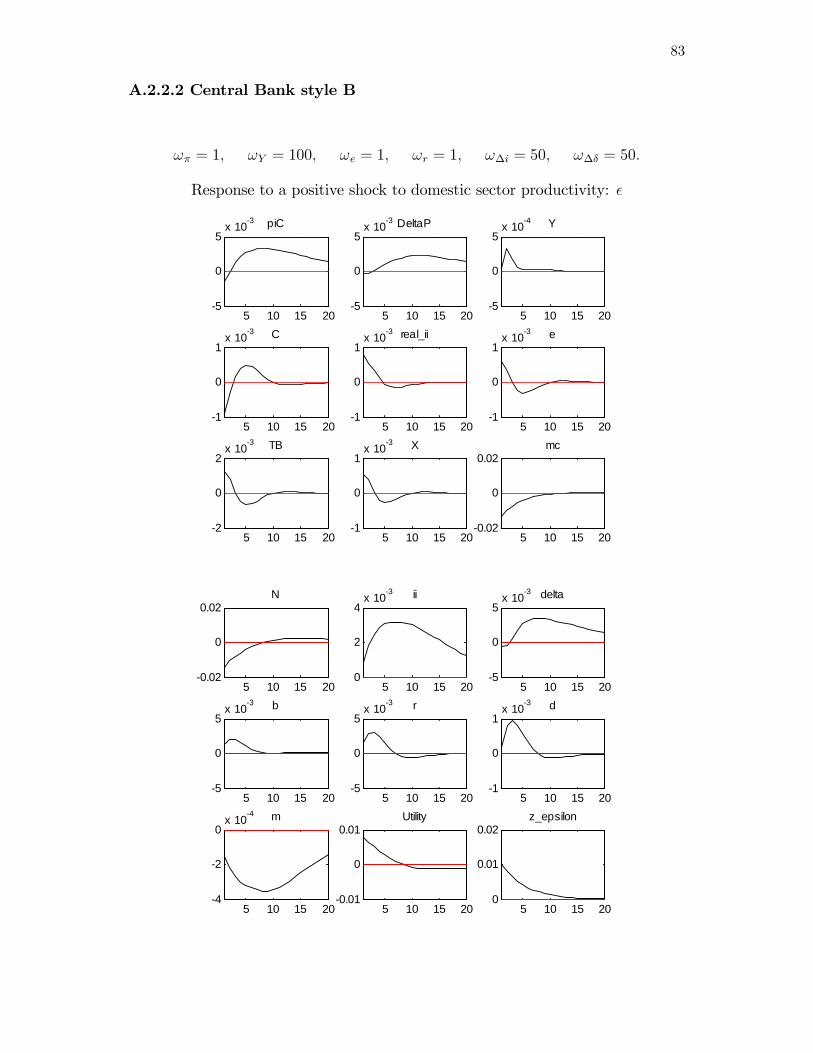
83
A.2.2.2 Central Bank style B
!� = 1; !Y = 100; !e = 1; !r = 1; !�i = 50; !�� = 50:
Response to a positive shock to domestic sector productivity: �
5 10 15 205
0
5x 10³ piC
5 10 15 205
0
5x 10³ DeltaP
5 10 15 205
0
5x 10⁴ Y
5 10 15 201
0
1x 10³ C
5 10 15 201
0
1x 10³ real_ii
5 10 15 201
0
1x 10³ e
5 10 15 202
0
2x 103 TB
5 10 15 201
0
1x 103 X
5 10 15 200.02
0
0.02mc
5 10 15 200.02
0
0.02N
5 10 15 200
2
4x 10³ ii
5 10 15 205
0
5x 10³ delta
5 10 15 205
0
5x 10³ b
5 10 15 205
0
5x 10³ r
5 10 15 201
0
1x 10³ d
5 10 15 204
2
0x 104 m
5 10 15 200.01
0
0.01Utility
5 10 15 200
0.01
0.02z_epsilon
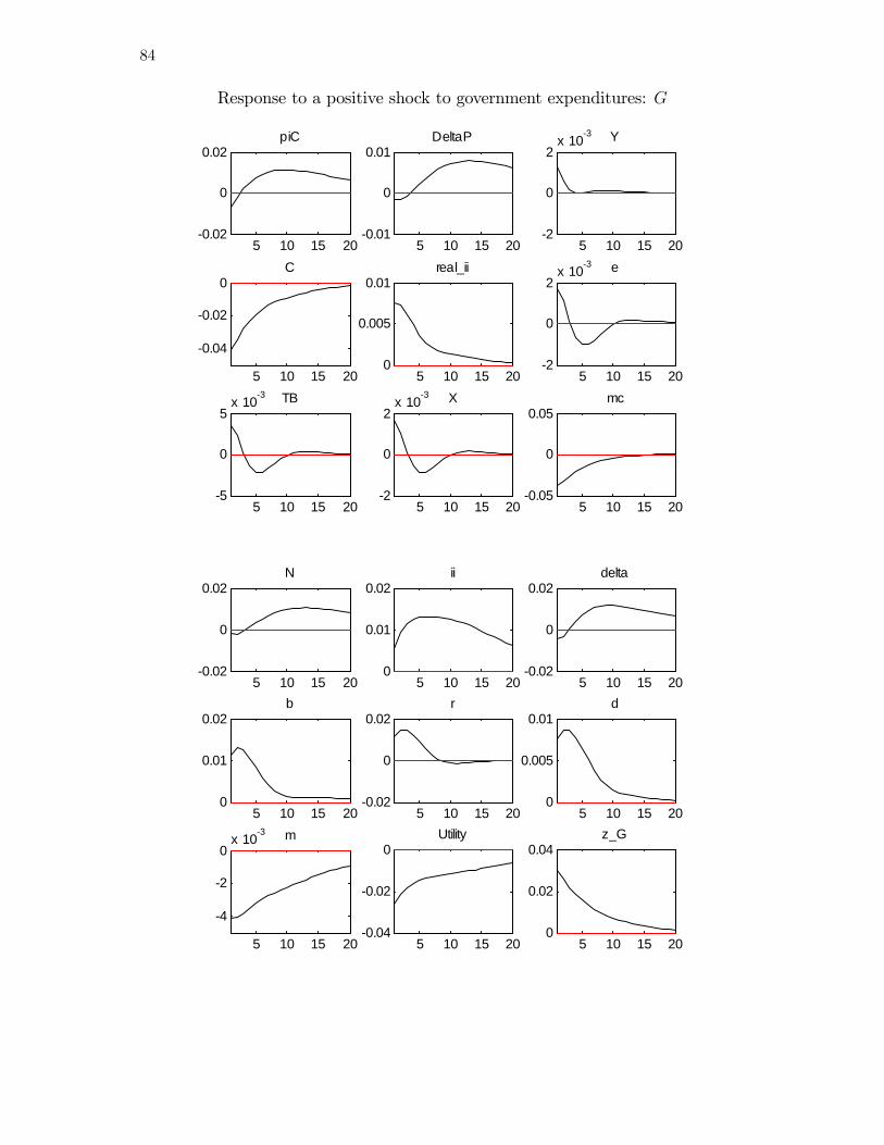
84
Response to a positive shock to government expenditures: G
5 10 15 200.02
0
0.02piC
5 10 15 200.01
0
0.01DeltaP
5 10 15 202
0
2x 10³ Y
5 10 15 20
0.04
0.02
0C
5 10 15 200
0.005
0.01real_ii
5 10 15 202
0
2x 10³ e
5 10 15 205
0
5x 103 TB
5 10 15 202
0
2x 103 X
5 10 15 200.05
0
0.05mc
5 10 15 200.02
0
0.02N
5 10 15 200
0.01
0.02ii
5 10 15 200.02
0
0.02delta
5 10 15 200
0.01
0.02b
5 10 15 200.02
0
0.02r
5 10 15 200
0.005
0.01d
5 10 15 20
4
2
0x 103 m
5 10 15 200.04
0.02
0Utility
5 10 15 200
0.02
0.04z_G

85
Response to a positive shock to the RW interest rate: i�
5 10 15 201
0
1x 10³ piC
5 10 15 205
0
5x 10⁴ DeltaP
5 10 15 205
0
5x 10⁴ Y
5 10 15 202
1
0x 103 C
5 10 15 205
0
5x 10⁴ real_ii
5 10 15 200
1
2x 10³ e
5 10 15 200
2
4x 103 TB
5 10 15 200
1
2x 103 X
5 10 15 202
0
2x 10³ mc
5 10 15 202
0
2x 10³ N
5 10 15 201
0
1x 10³ ii
5 10 15 201
0
1x 10³ delta
5 10 15 205
0
5x 10³ b
5 10 15 200.01
0
0.01r
5 10 15 200.01
0.005
0d
5 10 15 202
1
0x 104 m
5 10 15 201
0.5
0x 103 Utility
5 10 15 200
5x 10³z_iStar
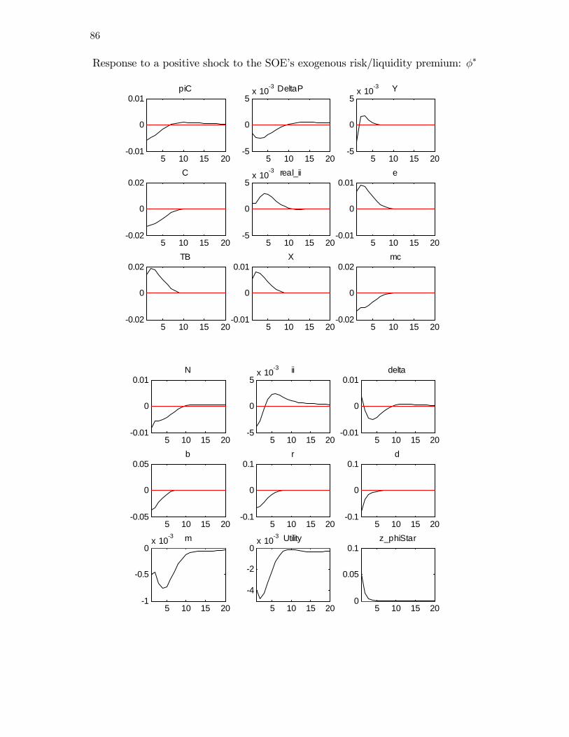
86
Response to a positive shock to the SOE�s exogenous risk/liquidity premium: ��
5 10 15 200.01
0
0.01piC
5 10 15 205
0
5x 10³ DeltaP
5 10 15 205
0
5x 10³ Y
5 10 15 200.02
0
0.02C
5 10 15 205
0
5x 10³ real_ii
5 10 15 200.01
0
0.01e
5 10 15 200.02
0
0.02TB
5 10 15 200.01
0
0.01X
5 10 15 200.02
0
0.02mc
5 10 15 200.01
0
0.01N
5 10 15 205
0
5x 10³ ii
5 10 15 200.01
0
0.01delta
5 10 15 200.05
0
0.05b
5 10 15 200.1
0
0.1r
5 10 15 200.1
0
0.1d
5 10 15 201
0.5
0x 103 m
5 10 15 20
4
2
0x 103 Utility
5 10 15 200
0.05
0.1z_phiStar
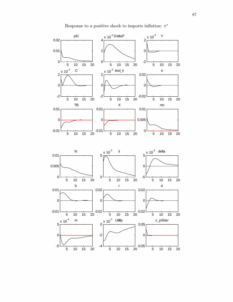
87
Response to a positive shock to imports in�ation: ��
5 10 15 200
0.01
0.02piC
5 10 15 200
2
4x 10³ DeltaP
5 10 15 202
0
2x 10³ Y
5 10 15 202
0
2x 10³ C
5 10 15 202
0
2x 10³ real_ii
5 10 15 200.02
0
0.02e
5 10 15 200.01
0
0.01TB
5 10 15 200.01
0
0.01X
5 10 15 200
0.005
0.01mc
5 10 15 200
0.005
0.01N
5 10 15 200
5x 10³ ii
5 10 15 205
0
5x 10³ delta
5 10 15 200.01
0
0.01b
5 10 15 200.02
0
0.02r
5 10 15 200.02
0
0.02d
5 10 15 205
0
5x 10⁴ m
5 10 15 204
2
0x 103 Utility
5 10 15 200.05
0
0.05z_piStar

88
Response to a positive shock to exports in�ation: ��X
5 10 15 200
0.01
0.02piC
5 10 15 200
0.005
0.01DeltaP
5 10 15 200.01
0
0.01Y
5 10 15 200.01
0
0.01C
5 10 15 205
0
5x 10³ real_ii
5 10 15 200.02
0
0.02e
5 10 15 200.02
0
0.02TB
5 10 15 200.02
0
0.02X
5 10 15 200.01
0
0.01mc
5 10 15 200
0.005
0.01N
5 10 15 200
0.01
0.02ii
5 10 15 200.02
0
0.02delta
5 10 15 200.05
0
0.05b
5 10 15 200.1
0
0.1r
5 10 15 200.05
0
0.05d
5 10 15 205
0
5x 10³ m
5 10 15 205
0
5x 10³ Utility
5 10 15 200.01
0
0.01z_piStar
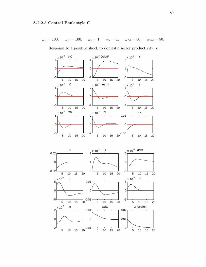
89
A.2.2.3 Central Bank style C
!� = 100; !Y = 100; !e = 1; !r = 1; !�i = 50; !�� = 50:
Response to a positive shock to domestic sector productivity: �
5 10 15 205
0
5x 10³ piC
5 10 15 201
0
1x 10³ DeltaP
5 10 15 200
1
2x 10³ Y
5 10 15 205
0
5x 10³ C
5 10 15 202
0
2x 10³ real_ii
5 10 15 202
0
2x 10³ e
5 10 15 205
0
5x 103 TB
5 10 15 202
0
2x 103 X
5 10 15 200.02
0
0.02mc
5 10 15 200.02
0
0.02N
5 10 15 200
1
2x 10³ ii
5 10 15 205
0
5x 10³ delta
5 10 15 205
0
5x 10³ b
5 10 15 200.01
0
0.01r
5 10 15 205
0
5x 10³ d
5 10 15 202
0
2x 10⁴ m
5 10 15 200.01
0
0.01Utility
5 10 15 200
0.01
0.02z_epsilon

90
Response to a positive shock to government expenditures: G
5 10 15 200.02
0
0.02piC
5 10 15 205
0
5x 10³ DeltaP
5 10 15 200
5x 10³ Y
5 10 15 20
0.04
0.02
0C
5 10 15 200
0.01
0.02real_ii
5 10 15 205
0
5x 10³ e
5 10 15 200.01
0
0.01TB
5 10 15 205
0
5x 103 X
5 10 15 200.05
0
0.05mc
5 10 15 200.01
0
0.01N
5 10 15 200
0.005
0.01ii
5 10 15 200.01
0
0.01delta
5 10 15 200.05
0
0.05b
5 10 15 200.05
0
0.05r
5 10 15 200
0.01
0.02d
5 10 15 20
4
2
0x 103 m
5 10 15 200.04
0.02
0Utility
5 10 15 200
0.02
0.04z_G

91
Response to a positive shock to the RW interest rate: i�
5 10 15 205
0
5x 10⁴ piC
5 10 15 202
0
2x 10⁴ DeltaP
5 10 15 205
0
5x 10⁴ Y
5 10 15 202
0
2x 10³ C
5 10 15 205
0
5x 10⁴ real_ii
5 10 15 200
1
2x 10³ e
5 10 15 200
2
4x 103 TB
5 10 15 200
1
2x 103 X
5 10 15 202
0
2x 10³ mc
5 10 15 201
0
1x 10³ N
5 10 15 201
0
1x 10³ ii
5 10 15 201
0
1x 10³ delta
5 10 15 204
2
0x 103 b
5 10 15 200.01
0.005
0r
5 10 15 200.01
0.005
0d
5 10 15 202
1
0x 104 m
5 10 15 201
0.5
0x 103 Utility
5 10 15 200
5x 10³z_iStar
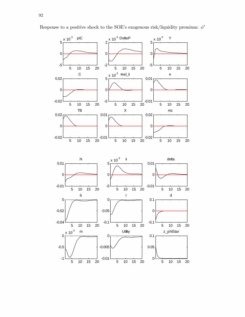
92
Response to a positive shock to the SOE�s exogenous risk/liquidity premium: ��
5 10 15 205
0
5x 10³ piC
5 10 15 202
0
2x 10³ DeltaP
5 10 15 205
0
5x 10³ Y
5 10 15 200.02
0
0.02C
5 10 15 205
0
5x 10³ real_ii
5 10 15 200.01
0
0.01e
5 10 15 200.02
0
0.02TB
5 10 15 200.01
0
0.01X
5 10 15 200.02
0
0.02mc
5 10 15 200.01
0
0.01N
5 10 15 205
0
5x 10³ ii
5 10 15 200.01
0
0.01delta
5 10 15 200.04
0.02
0b
5 10 15 200.1
0.05
0r
5 10 15 200.1
0
0.1d
5 10 15 201
0.5
0x 103 m
5 10 15 200.01
0.005
0Utility
5 10 15 200
0.05
0.1z_phiStar

93
Response to a positive shock to imports in�ation: ��
5 10 15 200.01
0
0.01piC
5 10 15 201
0
1x 10³ DeltaP
5 10 15 204
2
0x 104 Y
5 10 15 205
0
5x 10³ C
5 10 15 205
0
5x 10³ real_ii
5 10 15 200.02
0
0.02e
5 10 15 200.01
0
0.01TB
5 10 15 205
0
5x 103 X
5 10 15 205
0
5x 10³ mc
5 10 15 205
0
5x 10³ N
5 10 15 202
0
2x 10³ ii
5 10 15 200.01
0
0.01delta
5 10 15 200.02
0
0.02b
5 10 15 200.02
0
0.02r
5 10 15 200.02
0
0.02d
5 10 15 205
0
5x 10⁴ m
5 10 15 205
0
5x 10³ Utility
5 10 15 200.05
0
0.05z_piStar

94
Response to a positive shock to exports in�ation: ��X
5 10 15 205
0
5x 10³ piC
5 10 15 202
0
2x 10³ DeltaP
5 10 15 205
0
5x 10³ Y
5 10 15 200.01
0
0.01C
5 10 15 200.01
0
0.01real_ii
5 10 15 200.02
0
0.02e
5 10 15 200.05
0
0.05TB
5 10 15 200.02
0
0.02X
5 10 15 200.01
0
0.01mc
5 10 15 205
0
5x 10³ N
5 10 15 200.01
0
0.01ii
5 10 15 200.02
0
0.02delta
5 10 15 200.05
0
0.05b
5 10 15 200.1
0
0.1r
5 10 15 200.1
0
0.1d
5 10 15 202
0
2x 10³ m
5 10 15 200.01
0
0.01Utility
5 10 15 200.01
0
0.01z_piStar