a divide-and-merge methodology for clustering

A Divide-and-Merge Methodology for Clustering

DAVID CHENG

Massachusetts Institute of Technology

RAVI KANNAN

Yale University

SANTOSH VEMPALA


and

GRANT WANG


We present a divide-and-merge methodology for clustering a set of objects that combines a top-down “divide” phase with a bottom-up “merge” phase. In contrast, previous algorithms useeither top-down or bottom-up methods to construct a hierarchical clustering or produce a flatclustering using local search (e.g., k-means). For the divide phase, which produces a tree whoseleaves are the elements of the set, we suggest an efficient spectral algorithm. When the data isin the form of a sparse document-term matrix, we show how to modify the algorithm so that itmaintains sparsity and runs in linear space. The merge phase quickly finds the optimal partitionthat respects the tree for many natural objective functions, e.g., k-means, min-diameter, min-sum,correlation clustering, etc.. We present a thorough experimental evaluation of the methodology.We describe the implementation of a meta-search engine that uses this methodology to clusterresults from web searches. We also give comparative empirical results on several real datasets.

Categories and Subject Descriptors: H. Information Systems [H.3 Information Retrieval]:H.3.3 Information Search and Retreival

Additional Key Words and Phrases: Clustering, data mining, information retrieval

1. INTRODUCTION

The rapidly increasing volume of readily accessible data presents a challenge forcomputer scientists: find methods that can locate relevant information and organizeit in an intelligible way. This is different from the classical database problem inat least two ways: first, there may neither be the time nor (in the long term) thecomputer memory to store and structure all the data in a central location. Second,one would like to find interesting patterns in the data without knowing what tolook for in advance.

Clustering refers to the process of classifying a set of data objects into groupsso that each group consists of similar objects and objects from different groupsare dissimilar. The classification could either be flat (a partition of the data) orhierarchical [JD88]. Clustering has been proposed as a method to aid informationretrieval in many contexts (e.g. [CKPT92; VR79; SKK00; LA99; Dhi01]). Docu-ment clustering can help generate a hierarchical taxonomy efficiently (e.g. [Bol98;ZK02]) as well as organize the results of a web search (e.g. [ZEMK97; WF00]).It has also been used to learn (or fit) mixture models to datasets [Hof99] and forimage segmentation [TG97].

ACM Journal Name, Vol. V, No. N, July 2006, Pages 1–0??.

2 ·

merge

C2C1

C3

divide

Fig. 1. The Divide-and-Merge methodology

Most hierarchical clustering algorithms can be described as either divisive meth-ods (i.e. top-down) or agglomerative methods (i.e. bottom-up) [And73; JD88;JMF99]. Both methods create trees, but do not provide a flat clustering. A di-visive algorithm begins with the entire set and recursively partitions it into twopieces, forming a tree. An agglomerative algorithm starts with each object in itsown cluster and iteratively merges clusters. We combine top-down and bottom-uptechniques to create both a hierarchy and a flat clustering. In the divide phase,we can apply any divisive algorithm to form a tree T whose leaves are the objects.This is followed by the merge phase in which we start with each leaf of T in its owncluster and merge clusters going up the tree. The final clusters form a partition ofthe dataset and are tree-respecting clusters, i.e., they are subtrees rooted at somenode of T . For many natural objective functions, the merge phase can be executedoptimally, producing the best tree-respecting clustering. Figure 1 shows a depictionof the methodology.

For the divide phase we suggest using the theoretical spectral algorithm stud-ied in [KVV04]. The algorithm is well-suited for clustering objects with pairwisesimilarities – in [KVV04], the authors prove that the hierarchical tree formed bythe divide phase contains a “good clustering”. Unfortunately, the input to thatalgorithm is a matrix of pairwise similarities; for a dataset with n objects, the run-ning time could be O(n4). We describe an efficient implementation of the spectralalgorithm when the data is presented as a document-term matrix and the similarityfunction is the inner product. Note that the document-term matrix is often sparse,and thus is significantly smaller than the matrix of pairwise similarities; our im-plementation maintains the sparsity of the input. For a document-term matrix forn objects with M nonzeros, our implementation runs in O(Mn log n) in the worstcase and seems to perform much better in practice (see Figure 3(a)). The algorithmuses space linear in the number of nonzeros M . The data need not be text; all thatis needed is for the similarity of two objects to be the inner product between thetwo vectors representing the objects.

The class of functions for which the merge phase can find an optimal tree-respecting clustering include standard objectives such as k-means [HW79], min-diameter [CFM97], and min-sum [SG76], as well as correlation clustering, a for-mulation of clustering that has seen recent interest [BBC02; CGW03; DI03; EF03;ACM Journal Name, Vol. V, No. N, July 2006.

· 3

Swa04]. By optimal tree-respecting clustering, we mean that the clustering foundby the merge phase is optimal over the set of clusterings that respect the tree, i.e.clusterings whose clusters are nodes in the tree. Note that optimizing each of thestandard objective functions is NP-hard. Although approximation algorithms existfor these problems, many of them have impractical running times. Our methodol-ogy can be seen as an efficient alternative.

We conducted a thorough experimental evaluation for the methodology. Thefirst evaluation is in the form of a meta-search engine, EigenCluster [CKVW], thatclusters the results of a query to a standard web search engine. EigenClusterconsistently finds the natural clustering for queries that exhibit polysemy, e.g., forthe query monte carlo, EigenCluster finds clusters pertaining to the car model,the city in Monaco, and the simulation technique. We describe EigenCluster andshow results of example queries in Section 3.

We apply the methodology to clustering real-world datasets: text, gene expres-sion, and categorical data. In Section 4.2, we describe the results of a suite ofexperiments that test the effectiveness of the spectral algorithm as a procedure forthe divide phase. For these datasets, the “true” clustering is known in advance. Wecompare the “best” clustering in the tree built by the spectral algorithm to the trueclustering, where the “best” clustering in the tree is the one that most agrees withthe true clustering according to a variety of standard measures – f-measure, en-tropy, and accuracy. The results show that the spectral algorithm performs betterthan or competitively with several leading hierarchical clustering algorithms.

The results from Section 4.2 show that a good flat clustering exists in the treecreated by the divide phase. In Section 4.3, we give experimental results on theability of the merge phase to actually find this clustering that exists in the tree. Weexplore how some natural objective functions (k-means, min-sum, min-diameter)perform in practice on real-world data, and compare two flat clusterings: the clus-tering found by the objective function in the merge phase and the best clusteringthat exists in the tree. Our results show that the clustering found by the mergephase is only slightly worse than the best possible flat clustering in the tree.

2. DIVIDE-AND-MERGE METHODOLOGY

As mentioned in the introduction, there are two phases in our approach. The di-vide phase produces a hierarchy and can be implemented using any algorithm thatpartitions a set into two disjoint subsets. The input to this phase is a set of ob-jects whose pairwise similarities or distances are given, or can be easily computedfrom the objects themselves. The algorithm recursively partitions a cluster intotwo smaller sets until it arrives at singletons. The output of this phase is a treewhose leaves are the objects themselves; each internal node represents a subset ofthe objects, namely the leaves in the subtree below it. Divisive algorithms thatcan be applied in the divide phase are known for a variety of data representationssuch as graphs [Dhi01] and high-dimensional vectors [Bol98]. In Section 2.1, wesuggest a spectral algorithm analyzed in [KVV04] for the divide phase. We de-scribe an implementation that maintains sparsity of the data when the objects arerepresented as feature vectors and the similarity between the objects is the innerproduct between the corresponding vectors.

ACM Journal Name, Vol. V, No. N, July 2006.

4 ·

The merge phase is applied to the tree T produced by the divide phase. Theoutput of the merge phase is a partition C1, . . . , Ck of the set of objects and eachCi is a node of T . The merge phase uses a dynamic program to find the optimaltree-respecting clustering for a given objective function g. The optimal solutionsare computed bottom-up on T ; to compute the optimal solution for any interiornode C, we merge the optimal solutions for Cl and Cr, the children of C. Theoptimal solution for any node need not be just a clustering; an optimal solutioncan be parameterized in a number of ways. Indeed, we can view computing theoptimal solution for an interior node as computing a Pareto curve. A value on thecurve at a particular point is the optimal solution with the parameters describedby the point. A specific objective function g can be efficiently optimized on T ifthe Pareto curve for a cluster can be efficiently computed from the Pareto curves ofits children. The Pareto curve of the root node gives the tradeoff between the pa-rameters and the value of the objective function1. The choice of objective functionis up to the user and can be tailored to the specific application area. In Section2.2, we describe dynamic programs to compute optimal tree-respecting clusteringsfor several well-known objective functions: k-means, min-diameter, min-sum, andcorrelation clustering.

2.1 A spectral algorithm for the divide phase

In this section, we give an implementation of the spectral algorithm describedand analyzed in [KVV04]. The algorithm from [KVV04] takes as input a similaritymatrix encoding the similarity between objects and outputs a hierarchical clusteringtree. Our implementation deals with the common case where the objects are givenas feature vectors, and the similarity between the objects is defined to be the innerproduct of their feature vectors. Together, the objects form a sparse document-term matrix A ∈ Rn×m; the rows are the objects and the columns are the features.When A is sparse and n large, it is impractical to apply the spectral algorithm in[KVV04] as a black box. This is because explicitly computing the similarity matrixby computing the inner products takes n2 space, which can be much larger2 thanthe number of non-zeros M in the document-term matrix and thus infeasible tostore. The implementation we describe in this section takes as input the document-term matrix A and produces a hierarchical clustering tree with the same guaranteesas the algorithm from [KVV04]. The key benefit of our implementation is that ituses space linear in M and has a near-linear running time in M .

The algorithm constructs a hierarchical clustering of the objects by recursivelydividing a cluster C into two pieces through a cut (S, C \ S). To find the cut, wecompute v, an approximation of the second eigenvector of the similarity matrix AAT

normalized so that all row sums are 1. The ordering of the coordinates of v givesa set of n− 1 cuts, and we take the “best” cut (we describe what the “best” cut isin the next paragraph). The algorithm then recurses on the subparts. To computethe approximation of the second eigenvector, we use the power method, a technique

1For instance, the tradeoff might be between the number of clusters used and the amount of errorincurred – an example will be given for k-means in Section 2.2.2For instance, documents are often described in the bag-of-words model by their top-k distin-guishing features, with k < 500.


· 5

Input: An n×m matrix A.Output: A tree with the rows of A as leaves.

(1) Let ρ ∈ Rn be a vector of the row sums of AAT , and π = 1(P

i ρi)ρ.

(2) Let R, D be diagonal matrices with Rii = ρi, Dii =√

πi.

(3) Compute the second largest eigenvector v′ of Q = DR−1AAT D−1.

(4) Let v = D−1v′, and sort v so that vi ≤ vi+1.

(5) Find t such that the cut

(S, T ) = ({1, . . . , t}, {t + 1, . . . , n})

minimizes the conductance:

φ(S, T ) =c(S, T )

min(c(S), c(T ))

where c(S, T ) =P

i∈S,j∈T A(i) ·A(j), and c(S) = C(S, {1 . . . , n}).(6) Let AS , AT be the submatrices of A. Recurse (Steps 1-5) on AS and AT .

Table I. Divide phase

for which it is not necessary to explicitly compute the normalized similarity matrixAAT . We describe this in more detail in Section 2.1.1. The algorithm is given inTable I. There, we denote the ith object, a row vector in A, by A(i). The similarityof two objects is defined as the inner product of their term vectors: A(i) ·A(j).

In Step 5 of the algorithm, we consider n− 1 different cuts and use the cut withthe smallest conductance. Why should we think that the best cut is a cut of smallconductance? Why not just use the minimum cut (i.e. the cut with the minimumweight across it)? Consider Figure 2.1; the nodes are the objects and the edgesmean that two objects are very similar. Although both cut C1 and C2 have thesame number of edges crossing the cut, it is clear that C1 is a better cut – thisis because C1 partitions the set into two subsets of equal size, both of which havehigh weight. The measure of conductance formalizes this by normalizing a cut bythe smaller weight of the partition it induces. More intuition for why conductanceis a good measure for clustering can be found in [KVV04].

The cut (S, T ) we find using the second eigenvector in Step 5 is not the cut ofminimum conductance; finding such a cut is NP-hard. However, the conductance of(S, T ) is not much worse than the minimum conductance cut. Sinclair and Jerrumshowed that φ(S, T ) ≤

√2 · φOPT [SJ89; KVV04].

For a document-term matrix with n objects and M nonzeros, Steps 1-5 takeO(M log n) time. Theoretically, the worst-case time for the spectral algorithm tocompute a complete hierarchical clustering of the rows of A is O(Mn log n); thisoccurs if each cut the spectral algorithm makes only separates one object from therest of the objects. Experiments, however, show that the algorithm performs muchbetter (see Section 2.1.2). Indeed, if the spectral algorithm always makes balancedcuts, then the running time for creating a hierarchical clustering is O(M log2 n).We discuss this in more detail in Section 2.1.2.

Any vector or matrix that the algorithm uses is stored using standard data struc-tures for sparse representation. The main difficulty is to ensure that the similaritymatrix AAT is not explicitly computed; if it is, we lose sparsity and our runningtime could grow to n2. In the next section, we briefly describe how to avoid com-


6 ·

C1C2

Fig. 2. Minimum conductance cut vs. minimum cut

puting AAT in Steps 1 and 3. We also describe how to efficiently compute the n−1conductances in Step 5. By avoiding the computation of AAT , the algorithm runsin space O(M).

2.1.1 Details of the spectral algorithm.

2.1.1.1 Step 1: Computing row sums.. Observe that

ρi =n∑

j=1

A(i) ·A(j) =n∑

j=1

m∑k=1

AikAjk =m∑

k=1

Aik

n∑j=1

Ajk

.

Because∑n

j=1 Ajk does not depend on i, we can compute u =∑n

i=1 A(i) so wehave that ρi = A(i) · u. The total running time is O(M) and the additional spacerequired is O(n + m).

2.1.1.2 Step 3: Computing the eigenvector.. The algorithm described in [KVV04]uses the second largest eigenvector of B = R−1AAT , the normalized similarity ma-trix, to compute a good cut. To compute this vector efficiently, we compute thesecond largest eigenvector v of the matrix Q = DBD−1. The eigenvectors andeigenvalues of Q and B are related – if v is such that Bv = λv, then Q(Dv) = λDv.

The key property of Q is that it is a symmetric matrix. It is easy to see this fromthe fact that D2B = BT D2 and D is a diagonal matrix (so DT = D):

D2B = BT D2 → D−1D2B = D−1BT D2 → D−1D2BD−1 = D−1BT D2D−1 → Q = QT .

Since Q is symmetric, we can compute the second largest eigenvector of Q using thepower method, an iterative algorithm whose main computation is a matrix-vectormultiplication.

Power Method

(1) Let v ∈ Rn be a random vector orthogonal to πT D−1.ACM Journal Name, Vol. V, No. N, July 2006.

· 7

(2) Repeat(a) Normalize v, i.e. set v = v/||v||.(b) Set v = Qv.

Step 1 ensures that the vector we compute is the second largest eigenvector.Note that πT D−1Q = πT D−1, so πD−1 is a left eigenvector with eigenvalue 1.To evaluate Qv in Step 2, we only need to do four sparse matrix-vector multi-plications (v := D−1v, followed by v := AT v, v := Av, and v := DR−1v) sinceQ = (DR−1AAT D−1), and each of these matrices is sparse. Therefore, the spaceused is O(M), linear in the number of nonzeros in the document-term matrix A.

The following lemma shows that the power method takes O(log n) iterationsto converge to the top eigenvector. Although stated for the top eigenvector, thelemma and theorem still hold when the starting vector is chosen uniformly overvectors orthogonal to the top eigenvector πT D−1; in this case, the power methodwill converge to the second largest eigenvector (since the second eigenvector isorthogonal to the first). The analysis of the power method is standard and classical(see e.g. [GL96]). Our analysis differs in two respects. First, the classical analysisassumes that |λ1| > |λ2| – we do not need the assumption because if λ1 = λ2, the cutwe find partitions the graph into two pieces with no edges crossing the cut. Second,the classical analysis states convergence in terms of the size of the projection of thestarting vector on the first eigenvector; in our analysis, we quantify how large thisis for a random vector.

Lemma 1. Let A ∈ Rn×n be a symmetric matrix, and let v ∈ Rn be chosenuniformly at random from the unit n-dimensional sphere. Then for any positiveinteger k, the following holds with probability at least 1− δ:

||Ak+1v||||Akv||

≥(

n ln1δ

)− 12k

||A||2.

Proof. Since A is symmetric, we can write

A =n∑

i=1

λiuiuTi ,

where the λi ’s are the eigenvalues of A arranged in the order |λ1| ≥ |λ2| . . . |λn|and the ui are the corresponding eigenvectors. Note that, by definition, λ1 = ||A||2.Express v in this basis as v =

∑i αiui, where

∑i α2

i = 1. Since, v is uniformlyrandom over the unit-dimensional sphere, we have that with probability at least1 − δ, α2

1 ≥ 1/(n ln(1/δ)). It is easy to see that, in expectation, α21 = 1/n – this

follows from the symmetry of the sphere. The tail bound follows from the factthat the distribution of the projection of a point from the sphere to a random linebehaves roughly like a Gaussian random variable. Then, using Holder’s inequality(which says that for any p, q > 0 satisfying (1/p)+ (1/q) = 1 and any a, b ∈ Rn, wehave

∑i aibi ≤ (

∑i |ai|p)1/p (

∑i |bi|q)1/q), we have

||Akv||2 =∑

i

α2i λ

2ki ≤

(∑α2

i λ2k+2i

)k/(k+1)


8 ·

where the last inequality holds using Holder with p = 1 + (1/k) q = k + 1 ai =α

2k/(k+1)i λ2k

i bi = α2/(k+1)i . Note that ||Ak+1v|| =

∑i α2

i λ2k+2i . Combining this

with the previous inequality we have:

||Ak+1v||||Akv||

≥∑

i α2i λ

2k+2i(∑

α2i λ

2k+2i

)k/(k+1)≥(∑

α2i λ

2k+2i

)1/(k+1)

≥(α2

1λ2k+21

)1/(k+1).

As concluded above, with probability 1 − δ, α21 ≥ 1/(n ln(1/δ)). This gives us

the desired result.

The following corollary quantifies the number of steps to run the power methodto find a good approximation.

Corollary 1. If k ≥ 12ε ln(n ln( 1

δ )), then we have:

||Ak+1v||||Akv||

≥ (1− ε)λ1.

2.1.1.3 Step 5: Computing conductance of n − 1 cuts.. We choose the cut Cof the n − 1 cuts ({1, . . . , t}, {t + 1, . . . , n}) which has the smallest conductance.Recall that

φ({1, . . . , i}, {i + 1, . . . , n}) =

∑ik=1

∑nj=i+1 A(k) ·A(j)

min(∑i

k=1 ρk,∑n

k=i+1 ρk).

Let the numerator of this expression be ui, and the denominator be li.We can compute ui from ui−1 as follows. Let xi = A(1) + . . . + A(i) and yi =

A(i+1) + . . . + A(n). Then u1 = x1 · y1, and

ui = (xi−1 + A(i)) · (yi−1 −A(i)) = ui−1 − xi−1 ·A(i) + yi−1 ·A(i) + A(i) ·A(i).

The denominator, li can be computed in a similar fashion. Since we only requireone pass through A to compute the values of these n− 1 cuts, the time and spaceused is O(M).

2.1.2 Time and space requirements. In practice, the spectral algorithm does notrun in the worst-case O(Mn log n) time. If each cut made by the algorithm is bal-anced, then the spectral algorithm runs in O(M log2 n) time. By a balanced cut,we mean that both the number of nonzeros and number of rows on the larger sideof the cut are at most a constant fraction (say, 2/3) of the total number of nonze-ros and rows, respectively. If each cut is balanced, the depth of the hierarchicalclustering tree is at most O(log n). Since the running time at each level of thetree is M log n, the total running time when each cut is balanced is bounded aboveby O(M log2 n). On real world data, the algorithm seems to run in time roughlyO(M log5 n). Figures 3(a) and 3(b) show the results of a performance experiment.In this experiment, we computed a complete hierarchical clustering for N news-group articles in the 20 newsgroups dataset [Lan] and measured the running timeand memory used. The value of N ranged from 200 to 18,000. When we clustered18, 000 documents (for a total of 1.2 million nonzeros in the document-term ma-trix), we were able to compute a complete hierarchical clustering in 4.5 minutes onACM Journal Name, Vol. V, No. N, July 2006.

· 9

(a) Time vs. input size

(b) Space vs. input size

Fig. 3. Performance of spectral algorithm in experiments

commodity hardware (a 3.2 Ghz Pentium IV with 1 gigabyte of RAM). Note thatthe space used is linear in the size of the input.

In some applications, knowledge about the dataset can be used to halt the spectralalgorithm before a complete tree is constructed. For instance, if the number ofclusters k desired is small, the recursive step does not need to be applied afterdepth k, since all k-clusterings in the tree use nodes above depth k. Here is why– if a node t at depth k + 1 is a cluster, then no node along the path from t tothe root is also a cluster. Since each node along this path has two children, andeach leaf node must be covered by an interior node, there are at least k + 1 othernodes that need to be covered by distinct clusters, contradicting the use of only kclusters.


10 ·

2.2 Merge phase

The merge phase finds an optimal clustering in the tree produced by the dividephase. Recall that the tree produced by the divide phase has two properties: (1)each node in the tree is a subset of the objects, (2) the left and right children of anode form a partition of the parent subset. A clustering in the tree is thus a subsetS of nodes in the tree such that each leaf node is “covered”, i.e. the path from aleaf to root encounters exactly one node in S.

In this section, we give dynamic programs to compute the optimal clustering inthe tree for many standard objective functions. If we are trying to maximize theobjective function g, the dynamic program will find a clustering COPT-TREE inthe tree such that g(COPT-TREE) ≥ g(C), for any clustering C in the tree. Notethat the best clustering in the tree may not be the best possible clustering. Indeed,the best possible clustering may not respect the tree. In practice, we have foundthat good clusterings do exist in the tree created by the spectral algorithm andthat the merge phase, with appropriate objective functions, finds these clusterings(see Section 4.3).

In general, the running time of the merge phase depends on both the numberof times we must compute the objective function and the evaluation time of theobjective function itself. Suppose at each interior node we compute a Pareto curveof k points from the Pareto curves of the node’s children. Let c be the cost ofevaluating the objective function. Then the total running time is O(nk2 + nkc):linear in n and c, with a small polynomial dependence on k.

k-means: The k-means objective function seeks to find a k-clustering such thatthe sum of the squared distances of the points in each cluster to the centroid pi ofthe cluster is minimized:

g({C1, . . . , Ck}) =∑

i

∑u∈Ci

d(u, pi)2.

The centroid of a cluster is just the average of the points in the cluster. This problemis NP-hard; several heuristics (such as the k-means algorithm) and approximationalgorithms exist (e.g. [HW79; KSS04]). Let OPT-TREE(C, i) be the optimal tree-respecting clustering for C using i clusters. Let Cl and Cr be the left and rightchildren of C in T . Then we have the following recurrence:

OPT-TREE(C, 1) = {C}

since we are constrained to only use 1 cluster. When i > 1, we have:

OPT-TREE(C, i) = OPT-TREE(Cl, j) ∪ OPT-TREE(Cr, i− j)

where

j = argmin1≤j<i g(OPT-TREE(Cl, j) ∪ OPT-TREE(Cr, i− j)).

By computing the optimal clustering for the leaf nodes first, we can determinethe optimal clustering efficiently for any interior node. Then OPT-TREE(root, k)gives the optimal clustering. Note that in the process of finding the optimal clus-tering the dynamic program finds the Pareto curve OPT-TREE(root, ·); the curveACM Journal Name, Vol. V, No. N, July 2006.

· 11

describes the tradeoff between the number of clusters used and the “error” incurred.

Min-diameter: We wish to find a k-clustering for which the cluster with maximumdiameter is minimized:

g({C1, . . . , Ck}) = maxi

diam(Ci).

The diameter of any cluster is the maximum distance between any pair of objectsin the cluster. A similar dynamic program to that above can find the optimal tree-respecting clustering. This objective function has been investigated in [CFM97].

Min-sum: Another objective considered in the literature is minimizing the sum ofpairwise distances within each cluster:

g({C1, . . . , Ck}) =k∑

i=1

∑u,v∈Ci

d(u, v).

We can compute an optimal tree-respecting clustering in the tree T by a similardynamic program to the one above. Although approximation algorithms are knownfor this problem (as well as the one above), their running times seem too large tobe useful in practice [dlVKKR03].

Correlation clustering: Suppose we are given a graph where each pair of verticesis either deemed similar (red) or not (blue). Let R and B be the set of red and blueedges, respectively. Correlation clustering seeks to find a partition that maximizesthe number of agreements between a clustering and the edges – i.e. maximizing thenumber of red edges within clusters plus the number of blue edges between clusters:

g({C1 . . . Ck}) =∑

i

|{(u, v) ∈ R ∩ Ci}|+12|{(u, v) ∈ B : u ∈ Ci, v ∈ U \ Ci}|.

Let C be a cluster in the tree T , and let Cl and Cr be its two children. The dynamicprogramming recurrence for OPT-TREE(C) is:

OPT-TREE(C) = argmax {g(C), g(OPT-TREE(Cl) ∪ OPT-TREE(Cr)).

If, instead, we are given pairwise similarities in [0, 1], where 0 means dissimilar and 1means similar, we can define two thresholds t1 and t2. Edges with similarity greaterthan t1 are colored red and edges with similarity less than t2 are colored blue. Thesame objective function can be applied to these new sets of edges R(t1) and B(t2).Approximation algorithms have been given for this problem as well, although thetechniques used (linear and semidefinite programming) incur large computationaloverhead [BBC02; CGW03; DI03; EF03; Swa04].

2.3 Choice of algorithms for divide, merge steps

We have suggested a spectral algorithm for the divide phase and several differentobjective functions for the merge phase. A natural question is: how do these twophases interact, i.e. how does the choice of the algorithm for the divide phase affectthe performance of the merge phase?


12 ·

A natural approach is to use the same objective function for the divide phaseas the merge phase – that is, recursively find the optimal 2-clustering accordingto the objective function. This process results in a hierarchical clustering tree. Inthe merge phase, use the same objective function to find the best clustering. Inpractice, there can be difficulty with this approach because finding the optimal 2-clustering can be NP-hard as well (for instance, for the k-means, k-median objectivefunctions). Even if we could find the optimal 2-clustering, the hierarchical clusteringtree is not necessarily good for all k. This is the case for the min-diameter objectivefunction, where we seek a clustering that minimizes the maximum diameter betweentwo points in the same cluster. Consider the following four points on the realnumber line: 0, 1/2 − ε, 1/2 + ε, 1. The best 2-clustering is {0, 1/2 − ε}, {1/2 +ε, 1} with a maximum radius of 1/2 − ε. However, the optimal 3-clustering is{0}, {1/2 − ε, 1/2 + ε}, {1} with a maximum radius of 2ε, which does not respectthe initial partition. The best 3-clustering in the tree has maximum radius 1/2− ε,so the ratio of the best 3-clustering in the tree to the optimal 3-clustering cannotbe bounded by a constant. The situation is better for other objective functions.In the min k-cut objective function, we seek a k-clustering where the sum of thepairwise similarities across clusters is minimized. Saran and Vazirani show thatthe k-clustering obtained by greedily cutting the subset with the smallest min-cutk times is a factor 2 − 2/k approximation. The tree formed by recursively findingthe min-cut includes this greedy k-clustering, which gives the same factor 2− 2/kapproximation guarantee for the divide-and-merge methodology.

3. APPLICATION TO STRUCTURING WEB SEARCHES: EIGENCLUSTER

In a standard web search engine, the results for a given query are ranked in alinear order. Although suitable for some queries, the linear order fails to showthe inherent clustered structure of results for queries with multiple meanings. Forinstance, consider the query mickey. The query can refer to multiple people (MickeyRooney, Mickey Mantle) or the fictional character Mickey Mouse.

We have implemented the divide-and-merge methodology in a meta-search enginethat discovers the clustered structure for queries and identifies each cluster by itsthree most significant terms. The website is located at http://eigencluster.csail.mit.edu. The user inputs a query which is then used to find 400 results fromGoogle, a standard search engine. Each result contains the title of the webpage,its location, and a small snippet from the text of the webpage. We construct adocument-term matrix representation of the results; each result is a document andthe words in its title and snippet make up its terms. Standard text pre-processingsuch as TF/IDF, removal of stopwords, and removal of too frequent or infrequentterms is applied [VR79]. The similarity between two results is the inner productbetween their two term vectors.

The divide phase was implemented using our spectral algorithm. For the mergephase, we used the following objective function, which we refer to as relaxed corre-lation clustering:

∑i

α

∑u,v∈Ci

1−A(u) ·A(v)

+ β

∑u∈Ci,v /∈Ci

A(u) ·A(v)

.


· 13

We assume here that each row A(u) is normalized to have Euclidean length 1; thisis a standard preprocessing step that ensures that the maximum similarity betweenany pair of rows is 1. In EigenCluster, we use α = .2, and β = .8. The first term,α∑

u,v∈Ci(1 − A(u) · A(v)) measures the dissimilarity within a cluster, i.e. how

“far” a cluster is from a set in which every pair is as similar as possible (for all u, v,A(u) ·A(v) = 1). Note that the first term is a relaxed notion of the blue edges withina cluster from correlation clustering. The second term, β

∑u∈Ci,v /∈Ci

A(u) · A(v)

measures the amount of similarity the clustering fails to capture, since it occursacross clusters. Similarly, the second term is a relaxed notion of the red edgesoutside clusters. The benefit of using the relaxed correlation clustering objectivefunction is that it does not depend on a predefined number of clusters k. Thisis appropriate for our application, since the number of meanings or contexts of aquery could not possibly be known beforehand. We have seen in practice that theobjective function does a good job of picking out the large, interesting subsets ofthe data while putting unrelated results each in their own cluster.

Sample queries can be seen in Figures 4(a) and 4(c); in each example, EigenClus-ter identifies the multiple meanings of the query as well as keywords correspondingto those meanings. Furthermore, many results are correctly labeled as singletons.Figures 4(a) and 4(c) show screenshots of EigenCluster and Figures 4(b) and 4(d)are before and after depictions of the similarity matrix. The (i, j)th entry of thematrix represents the similarity between results i and j – the darker the pixel, themore similar i and j are. In the before picture, the results are arranged in theorder received from Google. In the after picture, the results are arranged accord-ing to the cuts made by the spectral algorithm. The cluster structure is apparent.EigenCluster takes roughly 0.7 seconds to fetch and cluster results on a PentiumIII 700 megahertz with 512 megabytes of RAM. Section 6 shows more exampleEigenCluster searches.

4. COMPARATIVE EXPERIMENTS ON STANDARD DATASETS

In this section, we conduct a thorough experimental evaluation of the divide-and-merge methodology. We work with real-world datasets (text, gene expression, andcategorical data) for which a labeling of data objects is known. In Section 4.2, weapply the spectral algorithm as a divide phase to the data. The results show thatthe tree the spectral algorithm constructs is good – there exists a clustering withinthe tree that “agrees” with the true clustering, i.e. the partition of data objectsinto sets whose members share the same label. This type of evaluation in whicha clustering algorithm is applied to data for which the true classification is knownis common. It is an appropriate evaluation because the true classification reflectsthe true structure of the data. Comparing the clustering found by the algorithmto the true classification measures the ability of a clustering algorithm to find truestructure in data, which is a primary use of clustering in practice. The results ofour experiments compare favorably to results obtained from leading hierarchicalclustering algorithms.

In Section 4.3, we proceed to experimentally evaluate the merge phase. Weevaluate how each of the objective functions k-means, min-sum, and min-diameterbehave on the tree constructed by the spectral algorithm. We find that the merge


14 ·

(a) Query: pods (b) Before/after: pods

(c) Query: mickey (d) Before/after: mickey

Fig. 4. Example EigenCluster searches

phase can indeed find a good clustering; it typically finds a clustering only slightlyworse than the “best” clustering that exists in the tree. The best clustering in thetree is the one that most closely matches the true clustering.

The next section describes how we compare a clustering (either hierarchical orflat) to the true clustering.ACM Journal Name, Vol. V, No. N, July 2006.

· 15

4.1 Comparative measures

Let the true classification of a dataset be C1, . . . , Ck. We refer to each Ci as aclass. Let C1, . . . , Cl be subsets of the universe U =

⋃i Ci. Note that C1, . . . , Cl

may have a non-empty intersection (for instance, when each Cl is the set of leavesunderneath a node of a hierarchical clustering tree). We will note when C1, . . . , Cl

is partition of U , rather than just a collection of subsets.

F -measure: For each class Ci, the F -measure of that class is:

F (i) =l

maxj=1

2PjRj

Pj + Rj

where:

Pj =|Ci ∩ Cj ||Ci|

, Rj =|Ci ∩ Cj ||Ci|

Pj is referred to as precision and Rj is referred to as recall. The F -measure of theclustering is defined as:

k∑i=1

F (i) · |Ci||C|

.

The F -measure score is in the range [0, 1] and a higher F -measure score implies abetter clustering. Note that the F -measure does not assume that C1, . . . , Cl is apartition of U ; indeed, it is often used to compare a hierarchical clustering to a trueclassification. For a more in-depth introduction and justification to the F -measure,see e.g. [VR79; LA99; BEX02; NJM01].

Entropy: We consider C1, . . . , Ck to be a partition of U . For each Cj , we definethe entropy of Cj as:

E(Cj) =k∑

i=1

−

(|Ci ∩ Cj ||Cj |

)log

(|Ci ∩ Cj ||Cj |

)The entropy of a subset is a measure of the disorder within the cluster. As such,a lower entropy score implies that a clustering is better; the best possible entropyscore is 0. Entropy was first introduced in [Sha48] and has been used as a measureof clustering quality in [Bol98; Dhi01; BLC02].

The entropy of a partition C1 . . . Ck is the weighted sum of the entropies of theclusters.

Accuracy: The accuracy of a partition C1, . . . , Ck is defined as:

maxπ∈Sk

∑ki=1 |Ci ∩ Cπ(i)|

|U |where Sk is the set of all permutations on k items. Note that the range of an accu-racy score is between 0 and 1; the higher the accuracy score, the better. Accuracy,which has been used as a measure of performance in supervised learning, has also


16 ·

dataset Spectral p-QR p-Kmeans K-meansalt.atheism 93.6 ± 2.6 89.3 ± 7.5 89.6 ± 6.9 76.3 ± 13.1

comp.graphicscomp.graphics 81.9 ± 6.3 62.4 ± 8.4 63.8 ± 8.7 61.6 ± 8.0

comp.os.ms-windows.miscrec.autos 80.3 ± 8.4 75.9 ± 8.9 77.6 ± 9.0 65.7 ± 9.3

rec.motorcyclesrec.sport.baseball 70.1 ± 8.9 73.3 ± 9.1 74.9 ± 8.9 62.0 ± 8.6rec.sport.hockey

alt.atheism 94.3 ± 4.6 73.7 ± 9.1 74.9 ± 8.9 62.0 ± 8.6sci.space

talk.politics.mideast 69.3 ± 11.8 63.9 ± 6.1 64.0 ± 7.2 64.9 ± 8.5talk.politics.misc

Table II. 20 Newsgroups dataset (Accuracy)

been used in clustering ([ST00], [ZDG+01]).

Confusion matrix: The confusion matrix for a partition C1, . . . , Ck shows thedistribution of the class of the objects in each Ci – it is a k×k matrix M where therows are the clusters Ci, and the columns are the classes Cj . The entry Mij denotesthe number of objects in Ci that belong to class Cj . The order of the clusters Ci

is chosen so as to maximize the number of elements on the diagonal.3

4.2 Spectral algorithm as the divide phase

We tested the spectral algorithm on three types of data: text, gene expression,and categorical data. In all experiments, we compare better than or favorably withthe known results. In each of the experiments, the known results come directlyas reported in the pertinent paper. To be precise, for each experiment, we ranthe same experiment as described in the pertinent paper, but with the spectralalgorithm instead of the algorithm given in the paper. In particular, we did nottry to validate the findings of each paper by rerunning the experiment with thealgorithm given in the paper.

4.2.1 Text data.

4.2.1.1 20 Newsgroups:. The 20 newsgroups resource [Lan] is a corpus of roughly20,000 articles that come from 20 specific Usenet newsgroups. We performed asubset of the experiments in [ZDG+01]. Each experiment involved choosing 50random newsgroup articles each from two newsgroups, constructing term vectorsfor them, and then applying the spectral algorithm to the document-term matrix.4

The term vectors were constructed exactly as in [ZDG+01]: words were stemmed,

3Maximizing the number of elements on the diagonal can be done via solving a maximum matchingproblem.4We used the BOW toolkit for processing the newsgroup data. More information on the BOWtoolkit can be found on http://www-2.cs.cmu.edu/∼mccallum/bow.


· 17

words that appear too few times were removed, and the TF/IDF weighting schemewas applied.

Since each experiment involved clustering documents from only two classes, wedid not need to form a complete hierarchical tree. The first cut made by the spectralalgorithm defines a partition into two clusters. Zha et al. also form two clustersusing their clustering algorithm. The results can be seen in Table II. Note thatwe perform better than p-QR, the algorithm proposed in [ZDG+01] on all but oneof the experiments. We also outperform K-means and a variation of the K-meansalgorithm, p-Kmeans. In each of these experiments, the measure of performance wasaccuracy. Since the experiment involved choosing 50 random newsgroup articles,the experiment was run 100 times and the mean and standard deviation of theresults were recorded.

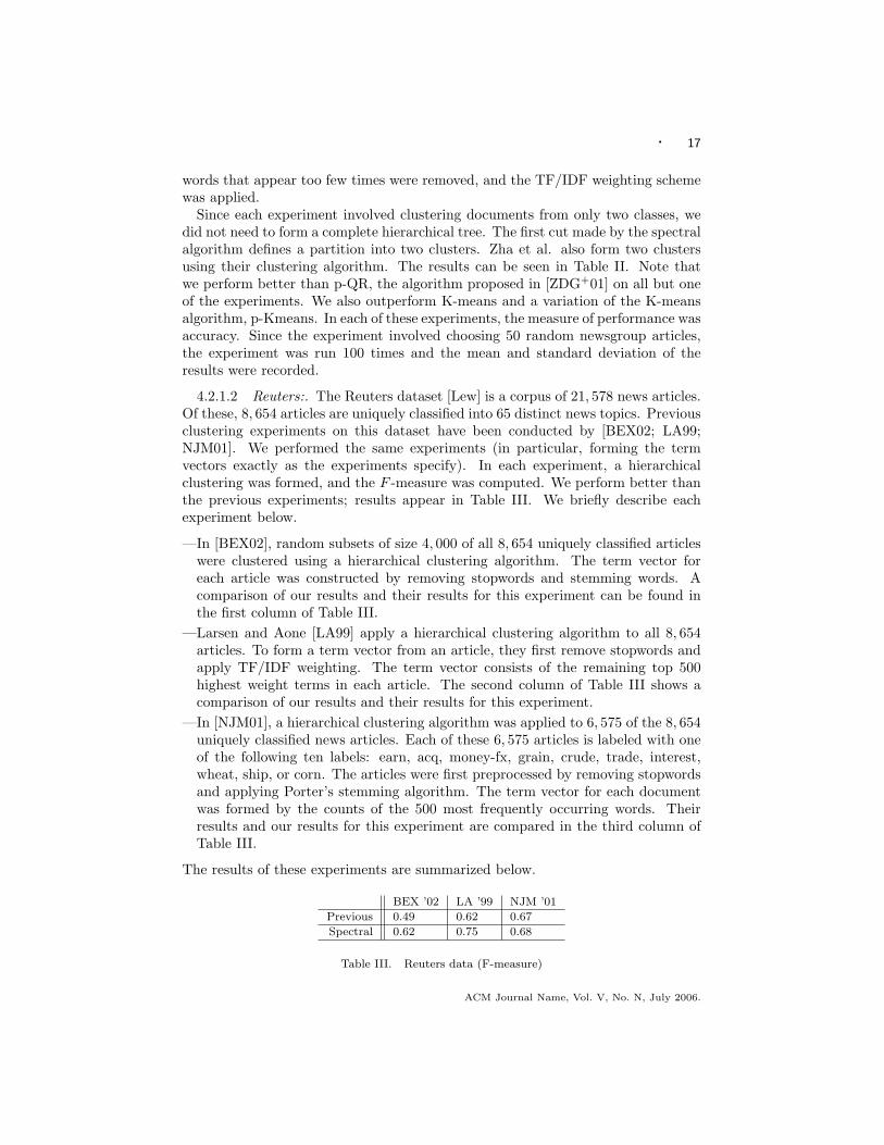
4.2.1.2 Reuters:. The Reuters dataset [Lew] is a corpus of 21, 578 news articles.Of these, 8, 654 articles are uniquely classified into 65 distinct news topics. Previousclustering experiments on this dataset have been conducted by [BEX02; LA99;NJM01]. We performed the same experiments (in particular, forming the termvectors exactly as the experiments specify). In each experiment, a hierarchicalclustering was formed, and the F -measure was computed. We perform better thanthe previous experiments; results appear in Table III. We briefly describe eachexperiment below.

—In [BEX02], random subsets of size 4, 000 of all 8, 654 uniquely classified articleswere clustered using a hierarchical clustering algorithm. The term vector foreach article was constructed by removing stopwords and stemming words. Acomparison of our results and their results for this experiment can be found inthe first column of Table III.

—Larsen and Aone [LA99] apply a hierarchical clustering algorithm to all 8, 654articles. To form a term vector from an article, they first remove stopwords andapply TF/IDF weighting. The term vector consists of the remaining top 500highest weight terms in each article. The second column of Table III shows acomparison of our results and their results for this experiment.

—In [NJM01], a hierarchical clustering algorithm was applied to 6, 575 of the 8, 654uniquely classified news articles. Each of these 6, 575 articles is labeled with oneof the following ten labels: earn, acq, money-fx, grain, crude, trade, interest,wheat, ship, or corn. The articles were first preprocessed by removing stopwordsand applying Porter’s stemming algorithm. The term vector for each documentwas formed by the counts of the 500 most frequently occurring words. Theirresults and our results for this experiment are compared in the third column ofTable III.

The results of these experiments are summarized below.

BEX ’02 LA ’99 NJM ’01

Previous 0.49 0.62 0.67

Spectral 0.62 0.75 0.68

Table III. Reuters data (F-measure)


18 ·

4.2.1.3 Web pages:. Boley [Bol98] performs a series of experiments on clustering185 webpages that fall into 10 distinct categories. In each of the 11 experiments (J1-J11), the term vector for each webpage was constructed in a slightly different way(the exact details can be found in [Bol98]5.). The algorithm from [Bol98] is also apartitional algorithm that constructs a hierarchical clustering. In each experiment,the quality of the clustering is measured by computing the entropy of the 16 clustersat depth 4 in the tree. We measured the entropy of the 16 clusters at depth 4 in ourtree as well as in an optimal partition into 16 clusters, allowing clusters at differentdepths. By an optimal partition into 16 clusters, we mean the 16-clustering in thetree that minimizes entropy. The results from [Bol98] appear in Table IV in therow “Boley ’98” and our results appear in the rows labeled “Fixed depth Spectral”(16 clusters at depth 4) and “Optimal Spectral” (optimal 16-clustering in the tree).

The results in Table IV show that the 16 clusters at depth 4 in our tree performbetter than the 16 clusters from [Bol98] in all but two experiments. The entropyof the best 16-clustering in the tree does markedly better than both “Fixed depthSpectral” and [Bol98]. This shows that a good clustering exists in the tree; we willsee that the merge phase can find a clustering almost as good as this in Section 4.3.

J1 J2 J3 J4 J5 J6 J7 J8 J9 J10 J11

Boley ’98 0.69 1.12 0.85 1.10 0.74 0.83 0.90 0.96 1.07 1.17 1.05

Fixed depth 0.77 0.92 0.72 0.94 0.76 0.72 0.84 0.88 0.89 1.04 0.88Spectral

Optimal 0.71 0.63 0.62 0.62 0.71 0.61 0.65 0.63 0.69 0.55 0.83Spectral

Table IV. Web page results (Entropy)

4.2.1.4 SMART dataset:. The SMART dataset is a set of abstracts originat-ing from Cornell University [Sal] that have been used extensively in informationretrieval experiments. The makeup of the abstracts is: 1,033 medical abstracts(Medline), 1,400 aeronautical systems abstracts (Cranfield), and 1,460 informationretrieval abstracts (Cisi). The term vector for each abstract was formed by remov-ing stopwords and words that occur in less than 0.2% or greater than 15% of theabstracts.

We performed the same four experiments as those found in [Dhi01]. In the firstthree experiments, the datasets were the mixture of abstracts from two classes. Inthe fourth experiment, the dataset was the set of all abstracts. In the first threeexperiments, we just apply the spectral algorithm once to obtain a 2-clustering ofthe data set. In the fourth experiment, we recurse with the spectral algorithmtwice, and select the better of the two 3-clusterings in the tree.

The results from performing the same experiments are listed in the column la-beled “Spectral” in Table V. We do much worse than [Dhi01]. The reason for thisis so many terms are removed in the construction of each term vector. As such,the similarity (inner product between two term vectors) may be very small, andthe best first conductance cut may separate just one or two objects from the rest

5The raw data can be found from ftp://ftp.cs.umn.edu/dept/users/boley/PDDPdata


· 19

dataset Spectral (TF/IDF) Spectral Dhillon ’01

MedCran 0.0172 0.027 0.026

MedCisi 0.0365 0.054 0.152

CisiCran 0.0426 0.490 0.046

Classic3 0.0560 0.435 0.089

Table V. SMART dataset (Entropy)

of the set. While the first cut may not separate the classes, we have found that oneof the next cuts often does separate the classes. When we applied TF/IDF weight-ing in the construction of term vectors, we found much better performance (seethe column labeled “Spectral (TF/IDF)” in Table V). Indeed, with TF/IDF termweighting, we perform better than [Dhi01]. The TF/IDF weighting increases theminimum similarity between any two abstracts, so that the best first conductancecut does not separate just one or two objects from the set.

4.2.2 Categorical data. Categorical data is similar in flavor to text data. How-ever, a data object is not a document containing terms, but rather a vector ofcharacteristics, each of which takes on non-numerical labels. A particular exam-ple is the Congressional voting dataset [UCI]. Each data object is a Congressman,and the vector of characteristics is how he voted on every bill or law put throughCongress. The true clustering of Congressmen is their political party affiliations.We show that our spectral algorithm can also be applied in this scenario. Again,only one cut is necessary as it defines a 2-clustering of the data. In Table VI, wesee that we do better than both COOLCAT [BLC02] and ROCK [GRS00].

Spectral COOLCAT ’02 ROCK ’000.480 0.498 0.499

Table VI. Congressional Voting Data (Entropy)

We also applied our algorithm to the Mushroom data set [UCI], which consistsof 8,124 mushrooms, each described by 22 features – such as odor (which takeson values such as almond, anise, creosote) and habitat (which takes on valuessuch as grasses, leaves, or meadows). We represented each mushroom as a vectorand each possible value as a coordinate. Thus, each mushroom is described by abinary vector. Each mushroom is labeled either poisonous or edible; we considerthis the true clustering of the data. The COOLCAT and ROCK algorithms havebeen applied to this dataset by [ATMS04], who also introduce LIMBO, a categoricalclustering algorithm, and apply it to this dataset. In Table VII, we show the resultsof the experiment. The precision and recall were measured; we perform better thanROCK and COOLCAT in both measures, but LIMBO outperforms us in bothmeasures.

4.2.3 Gene expression data. A microarray chip is a solid surface upon whichspots of DNA are attached in a matrix-like configuration. By exposing the chipto RNA, the expression level (roughly the activity of the gene) can be determined


20 ·Spectral COOLCAT ’02 ROCK ’00 LIMBO ’04

Precision 0.81 0.76 0.77 0.91Recall 0.81 0.73 0.57 0.89

Table VII. Mushroom Data

for each gene on the microarray chip. A seminal paper [GST+99] proposed anapproach to discovering new subtypes of cancer by clustering microarray data. Theapproach is to cluster gene expression data from several patients with a certaintype of cancer. If a strong clustering exists, the clustering might designate differentsubtypes of cancer. This relies on the the hypothesis that gene expression levelscan distinguish different subtypes of cancer.

They tested the validity of this approach by applying it to a known sub-classificationof leukemia. Two distinct subtypes of leukemia are: acute lymphoblastic leukemia(ALL) and acute myeloid leukemia (AML). Golub et al. asked: could the approachto cancer classification correctly find the two known subtypes of ALL and AML?To this end, they prepared microarray chips for 38 bone marrow samples. Eachchip contained roughly 7,000 human genes. Each bone marrow sample came fromeither one of 27 ALL patients or 11 AML patients. The gene expression data thuscan be described by a 38 by 7,000 matrix M . Golub et al. clustered the 38 rowvectors of this matrix using self-organizing maps [TSM+99]. The confusion matrixof their clustering is shown in Table VIII.

ALL AMLC1 26 1C2 1 10

Table VIII. Confusion matrix for Golub et al. clustering

The clustering (C1, C2) almost exactly obeys the ALL/AML distinction. Golubet al. also provide a list of genes that are highly expressed in C1, but not in C2, andvice versa – they posit that the expression level of these genes distinguish betweenAML and ALL.

We ran the spectral algorithm on the gene expression data [Gol], which we pre-processed as follows. First, the data was normalized: the expression level of eachgene was normalized over the 38 samples such that the mean was zero and thestandard deviation was one.6 Then, we created a 38 by 14,000 matrix N ; thejth column in the original gene expression matrix, M(·, j) corresponds to the twocolumns N(·, 2j−1) and N(·, 2j). The two columns in N separate the negative andpositive values in M : if M(i, j) < 0, then N(i, 2j−1) = |M(i, j)| and if M(i, j) > 0,then N(i, 2j) = M(i, j). The similarity between two samples (i.e. two rows of N)is just the inner product. Thus, if two samples have a large inner product, theyhave a similar gene expression profile. The confusion matrix for the first cut foundby the spectral algorithm is shown in Table IX.

6Golub et al. do the same normalization


· 21

ALL AMLC3 18 1C4 9 10

Table IX. Confusion matrix for Spectral 2-clustering

While C3 is almost a pure ALL cluster, the clustering (C3, C4) does not obeythe ALL/AML class boundary. Interestingly, recursing on the cluster C4 gives a3-clustering that does obey the ALL/AML class boundary. Table X shows theconfusion matrix for this 3-clustering.

ALL AMLC3 18 1C5 0 10C6 9 0

Table X. Confusion matrix for Spectral 3-clustering

A random 3-clustering does not obey the class boundary, so clearly the 3-clusteringfound by the spectral algorithm obeys the natural properties of the data. But whydoes the 2-clustering found by the spectral algorithm not respect this distinction?Preliminary investigations suggest that the 2-clustering finds distinguishing genesthat are more statistically significant than the Golub clustering; it seems worthwhileto fully investigate the biological significance of this finding.

4.3 Merge phase in practice

The experiments in Section 4.2 imply that a good clustering exists in the tree cre-ated by the spectral algorithm. When the number of desired clusters k is small (i.e.in the SMART dataset or the 20 newsgroups dataset), finding a good k-clusteringin the tree is not difficult. The only 2-clustering in a hierarchical clustering tree isthe first partition, and there are only two 3-clusterings to examine. However, whenthe number of desired clusters is high, there are an exponential number of possibleclusterings.

The Boley webpage dataset and Reuters dataset provide a good test for the mergephase, since the number of true clusters in these datasets is high. We show that forthese datasets, the objective functions find a good flat clustering in the tree.

4.3.0.1 Web pages:. Recall that the Boley dataset consists of 185 webpages, eachof which fall into 10 distinct classes. Section 4.2 showed that a good 16-clusteringof the dataset exists in the tree.

We ran the same experiments J1-J11 on this dataset, but after constructing thetree via the spectral algorithm in the divide phase, we applied dynamic programsfor three different objective functions (k-means, min-sum and min-diameter7) in the

7We did not apply the correlation clustering objective function, because we cannot control thenumber of clusters it finds. Any comparison to an objective function with a fixed number of


22 ·

merge phase. We set k, the number of clusters desired, to 10. We also determinedthe 10-clustering in the tree with the lowest entropy. The results appear in TableXI. We see that k-means and min-sum generally perform better than min-diameter.What is most interesting is that the clustering obtained by either min-sum or k-means is only slightly worse than the best clustering in the tree. Indeed, in 7of 11 experiments, the clustering obtained by min-sum or k-means was exactlythe best clustering in the tree. Table XII shows the confusion matrix from theclustering obtained in experiment J4. All classes except for C9 and C10 have aclear corresponding cluster Ci. The weight on the diagonal is 131, meaning that131/185 ≈ 71% of the articles are correctly classified.

J1 J2 J3 J4 J5 J6 J7 J8 J9 J10 J11

k-means 1.00 0.93 0.88 0.81 1.00 0.93 0.84 0.83 0.95 0.71 1.07

min-sum 0.98 0.93 0.88 0.78 0.98 0.92 0.84 0.83 0.94 0.71 1.10

min-diam 1.04 1.10 0.96 1.04 1.10 1.00 1.05 1.23 1.24 0.83 1.16

best in tree 0.98 0.93 0.88 0.78 0.96 0.91 0.84 0.83 0.92 0.71 1.05

Table XI. Webpage dataset: Objective function performance in the merge phase (Entropy)

C1 C2 C3 C4 C5 C6 C7 C8 C9 C10

C1 18 0 3 0 1 0 1 0 0 0

C2 0 17 0 0 0 2 0 0 0 0

C3 0 1 13 2 0 0 0 0 0 1

C4 0 0 0 10 0 0 0 1 7 1

C5 0 0 0 0 18 0 1 0 0 0

C6 0 1 0 0 0 13 1 0 0 0

C7 0 0 1 3 0 1 15 0 0 0

C8 0 0 1 0 0 0 0 12 0 0

C9 1 0 0 2 1 0 1 4 3 3

C10 0 0 1 2 0 0 0 2 8 12

Table XII. Webpage dataset: Confusion matrix for min-sum clustering on experiment J4

4.3.0.2 Reuters:. The Reuters dataset also contains a large number of classes –8, 654 of the 21, 578 articles are uniquely assigned to 65 labels. We chose all 1, 832articles that were assigned to the following 10 labels: coffee, sugar, trade, ship,money-supply, crude, interest, money-fx, gold, or gnp. We formed term vectorsby removing stopwords and stemming words. We also removed all words thatoccur in less than 2% of the articles or more than 50% of the articles. A completehierarchical tree was computed in the divide phase using the spectral algorithm,and we used dynamic programs in the merge phase to compute flat clusterings forthe k-means, min-sum, and min-diameter objective functions, for k = 10, 15 and20. The results appear in Table XIII. We do not perform as well as in the webpage

clusters would be unfair.


· 23

dataset. However, the entropy of the clusterings found by k-means and min-sumare not too far from the entropy of the best clustering in the tree.

We give the confusion matrix for the k-means clustering for k = 10 in Table XIV;only C4, C5, C7, and C10 do not clearly correspond to any class. The weight alongthe diagonal is 1068, meaning that 1068/1832 ≈ 58% of the articles are correctlyclassified.

k = 10 k = 15 k = 20

k-means 1.02 0.92 0.84

min-sum 1.05 0.90 0.79

min-diam 1.10 0.94 0.80

best in tree 0.99 0.84 0.76

Table XIII. Reuters dataset: Objective function performance in the merge phase (Entropy)

C1 C2 C3 C4 C5 C6 C7 C8 C9 C10

C1 96 4 3 19 0 0 0 0 0 1

C2 0 109 0 9 0 0 0 0 0 0

C3 4 1 203 29 0 4 1 8 0 2

C4 0 6 2 71 0 100 0 2 0 0

C5 2 2 59 3 75 13 11 11 2 15

C6 0 0 0 3 0 198 0 0 0 0

C7 1 0 55 5 7 14 160 148 0 49

C8 0 0 0 1 1 1 0 60 0 0

C9 3 4 1 5 0 5 0 1 90 0

C10 8 9 10 11 14 20 39 29 7 6

Table XIV. Reuters dataset: Confusion matrix for k-means experiment with k = 10

5. CONCLUSION

We have presented a divide-and-merge methodology for clustering, and shown anefficient and effective spectral algorithm for the divide phase. For the merge phase,we have described dynamic programming formulations that compute the optimaltree-respecting clustering for standard objective functions. A thorough experimen-tal evaluation of the methodology shows that the technique is effective on real-worlddata.

This work raises several additional questions: are the tree-respecting clusterings(for a suitable choice of objective function) provably good approximations to theoptimal clusterings? Does the tree produced by the spectral algorithm contain aprovably good clustering? Which objective functions are more effective at findingthe true clustering in the tree in practice?


24 ·

REFERENCES

M. Anderberg. Cluster Analysis for Applications. Academic Press, 1973.

Periklis Andritsos, Panayiotis Tsaparas, Rene J. Miller, and Kenneth C. Sevcik. Limbo: Scalableclustering of categorical data. In International Conference on Extending Database Technology,2004.

N. Bansal, A. Blum, and S. Chawla. Correlation clustering. In Proceedings of the 43rd IEEESymposium on Foundations of Computer Science, pages 238–247, 2002.

F. Beil, M. Ester, and X. Xu. Frequent term-based text clustering. In Proceedings of the eighthACM SIGKDD international conference on Knowledge discovery and data mining, pages 436–442, 2002.

D. Barbara, Y. Li, and J. Couto. Coolcat: an entropy-based algorithm for categorical cluster-ing. In Proceedings of the eleventh international conference on Information and knowledgemanagement, pages 582–589, 2002.

D. Boley. Principal direction divisive partitioning. Data Mining and Knowledge Discovery,2(4):325–344, 1998.

C. Chekuri, T. Feder, and R. Motwani. Incremental clustering and dynamic information retrieval.In Proceedings of the 29th Annual ACM Symposium on Theory of Computing, pages 626–635,1997.

M. Charikar, V. Guruswami, and A. Wirth. Clustering with qualitative information. In Pro-ceedings of the 44th Annual IEEE Symposium on Foundations of Computer Science, pages524–533, 2003.

D. R. Cutting, D. R. Karger, J. O. Pedersen, and J. W. Tukey. Scatter/gather: a cluster-basedapproach to browsing large document collections. In Proceedings of the 15th annual interna-tional ACM SIGIR conference on Research and development in information retrieval, pages318–329, 1992.

D. Cheng, R. Kannan, S. Vempala, and G. Wang. Eigencluster. http://eigencluster.csail.

mit.edu.

I. S. Dhillon. Co-clustering documents and words using bipartite spectral graph partitioning. InProceedings of the seventh ACM SIGKDD international conference on Knowledge discoveryand data mining, pages 269–274, 2001.

E.D. Demaine and N. Immorlica. Correlation clustering with partial information. In Proceedings ofthe 6th International Workshop on Approximation Algorithms for Combinatorial OptimizationProblems, pages 1–13, 2003.

W.F. de la Vega, M. Karpinski, C. Kenyon, and Y. Rabani. Approximation schemes for clusteringproblems. In Proceedings of the 35th Annual ACM Symposium on Theory of Computing, pages50–58, 2003.

D. Emanuel and A. Fiat. Correlation clustering–minimizing disagreements on arbitrary weightedgraphs. In Proceedings of the 11th European Symposium on Algorithms, pages 208–220, 2003.

G. H. Golub and C. F. Loan. Matrix Computations. Johns Hopkins, third edition, 1996.

T. R. Golub. Golub leukemia data.

Sudipto Guha, Rajeev Rastogi, and Kyuseok Shim. ROCK: A robust clustering algorithm forcategorical attributes. Information Systems, 25(5):345–366, 2000.

T. R. Golub, D. K. Slonim, P. Tamayo, C. Huard, M. Gaasenbeek, J. P. Mesirov, H. Coller,M. L. Loh, J. R. Downing, M. A. Caligiuri, C. D. Bloomfield, and E. S. Lander. Molecularclassification of cancer: Class discovery and class prediction by gene expression monitoring.Science, 286:531–537, 1999.

T. Hofmann. The cluster-abstraction model: Unsupervised learning of topic hierarchies from textdata. In International Joint Conference on Artificial Intelligence, pages 682–687, 1999.

J.A. Hartigan and M.A. Wong. A k-means clustering algorithm. In Applied Statistics, pages100–108, 1979.

A. Jain and R. Dubes. Algorithms for Clustering Data. Prentice Hall, 1988.

A. Jain, M. Murty, and P. Flynn. Data clustering: A review. ACM Computing Surveys, 31, 1999.


· 25

A. Kumar, S. Sen, and Y. Sabharwal. A simple linear time (1+ε)-approximation algorithm fork-means clustering in any dimensions. In Proceedings of the 45th Annual IEEE Symposium onFoundations of Computer Science, pages 454–462, 2004.

R. Kannan, S. Vempala, and A. Vetta. On clusterings: Good, bad, and spectral. Journal of theACM, 51(3):497–515, 2004.

B. Larsen and C. Aone. Fast and effective text mining using linear-time document clustering. InProceedings of the fifth ACM SIGKDD international conference on Knowledge discovery anddata mining, pages 16–22, 1999.

K. Lang. 20 newsgroups data set. http://www.ai.mit.edu/people/jrennie/20Newsgroups/.

D. Lewis. Reuters data set. http://www.daviddlewis.com/resources/testcollections/

reuters21578/.

A. Nickerson, N. Japkowicz, and E. Milios. Using unsupervised learning to guide re-samplingin imbalanced data sets. In Proceedings of the Eighth International Workshop on AI andStatitsics, pages 261–265, 2001.

G. Salton. SMART Data Set. ftp://ftp.cs.cornell.edu/pub/smart.

S. Sahni and T. Gonzalez. P-complete approximation problems. Journal of the ACM, 23(3):555–566, 1976.

C. E. Shannon. A mathematical theory of communication. Bell Systems Technical Journal,27:379–423, 1948.

A. Sinclair and M. Jerrum. Approximate counting, uniform generation, and rapidly mixing markovchains. Information and Computation, 82:93–133, 1989.

M. Steinbach, G. Karypis, and V. Kumar. A comparison of document clustering techniques. InKDD Workshop on Text Mining, 2000.

N. Slonim and N. Tishby. Document clustering using word clusters via the information bottleneckmethod. In Proceedings of the 23d Annual International ACM Conference on Research andDevelopment in Information Retrieval, pages 208–215, 2000.

C. Swamy. Correlation clustering: Maximizing agreements via semidefinite programming. InProceedings of ACM-SIAM Symposium on Discrete Algorithms, pages 519–520, 2004.

J. Theiler and G. Gisler. A contiguity-enhanced k-means clustering algorithm for unsupervisedmultispectral image segmentation. In Proceedings of the Society of Optical Engineering, pages108–111, 1997.

P. Tamayo, D. Slonim, J. Mesirov, Q. Zhu, S. Kitareewan, E. Dmitrovsky, E. Lander, andT. Golub. Interpreting patterns of gene expression with self-organizing maps; methods andapplication to hematopoietic differentiation. Proc. Nat. Acad. Sci, 96:2907–2912, 1999.

UCI. UCI Machine Learning Repository. http://www.ics.uci.edu/∼mlearn/MLRepository.html.

C. J. Van Rijsbergen. Information Retrieval, 2nd edition. Dept. of Computer Science, Universityof Glasgow, 1979.

W. Wong and A. Fu. Incremental document clustering for web page classification. In IEEEInternational Conference on Information Society in the 21st Century: Emerging Technologiesand New Challenges, 2000.

H. Zha, C. Ding, M. Gu, X. He, and H. Simon. Spectral relaxation for k-means clustering. InNeural Information Processing Systems, pages 1057–1064, 2001.

O. Zamir, O. Etzioni, O. Madani, and R. M. Karp. Fast and intuitive clustering of web documents.In Proceedings of the 3rd International Conference on Knowledge Discovery and Data Mining,pages 287–290, 1997.

Y. Zhao and G. Karypis. Evaluation of hierarchical clustering algorithms for document datasets.In Proceedings of the Eleventh International Conference on Information and Knowledge Man-agement, pages 515–524, 2002.

6. EIGENCLUSTER EXAMPLE SEARCHES


26 ·

(a) Query: trees (b) Before/after: trees

(c) Query: bears (d) Before/after: bears

Fig. 5. Example EigenCluster searches


a divide-and-merge methodology for clustering

Documents