a divergence-form wave-induced pressure inherent in the … · 2015-07-09 · a divergence-form...

A Divergence-Form Wave-Induced Pressure Inherent in the Extensionof the Eliassen–Palm Theory to a Three-Dimensional Framework

for All Waves at All Latitudes*

HIDENORI AIKI

Application Laboratory, Japan Agency for Marine-Earth Science and Technology, Yokohama, Japan

KOUTAROU TAKAYA

Department of Physics, Faculty of Science, Kyoto Sangyo University, Kyoto, Japan

RICHARD J. GREATBATCH

GEOMAR Helmholtz-Zentrum f€ur Ozeanforschung Kiel, Kiel, Germany

(Manuscript received 17 June 2014, in final form 20 January 2015)

ABSTRACT

Classical theory concerning theEliassen–Palm relation is extended in this study to allow for a unified treatment

of midlatitude inertia–gravity waves (MIGWs), midlatitude Rossby waves (MRWs), and equatorial waves

(EQWs). A conservation equation for what the authors call the impulse-bolus (IB) pseudomomentum is useful,

because it is applicable to ageostrophic waves, and the associated three-dimensional flux is parallel to the direction

of the group velocity of MRWs. The equation has previously been derived in an isentropic coordinate system or

a shallow-water model. The authors make an explicit comparison of prognostic equations for the IB pseudo-

momentum vector and the classical energy-based (CE) pseudomomentum vector, assuming inviscid linear waves

in a sufficiently weak mean flow, to provide a basis for the former quantity to be used in an Eulerian time-mean

(EM) framework. The authors investigate what makes the three-dimensional fluxes in the IB and CE pseudo-

momentum equations look in different directions. It is found that the two fluxes are linked by a gauge trans-

formation, previously unmentioned, associated with a divergence-form wave-induced pressureL. The quantityLvanishes for MIGWs and becomes nonzero for MRWs and EQWs, and it may be estimated using the virial

theorem. Concerning the effect of waves on the mean flow, L represents an additional effect in the pressure

gradient term of both (the three-dimensional versions of) the transformed EM momentum equations and the

merged form of the EMmomentum equations, the latter of which is associatedwith the nonacceleration theorem.

1. Introduction

Generalization of classical wave–mean flow interaction

theory concerning the Eliassen–Palm relation has attracted

significant attention in the past decades (Eliassen and Palm

1960; Bühler 2014). The theory was originally developedin a zonal-mean framework for mountain waves and

reformulated by Andrews and McIntyre (1976, hereafter

AM76) in the context of quasigeostrophic dynamics. Let A

and Ay [A2A be the zonal mean (at fixed latitude and

height) of an arbitrary quantityA and the deviation from it,

respectively. A zonal-mean quasigeostrophic expression for

the Taylor–Bretherton identity (Taylor 1915; Bretherton

1966; Dritschel and McIntyre 2008) may be written as

yyQy5›yFy1›zF

z , (1a)

Fy[ cxcy52yyuy, and (1b)

Fz[ 2(czcx= rz)f20 r0=g5 ry›xpy= rz5 f0r

yyy=rz ,(1c)

* Supplemental information related to this paper is available at the

Journals Online website: http://dx.doi.org/10.1175/JAS-D-14-0172.s1.

Corresponding author address: Hidenori Aiki, JAMSTEC,

3173-25, Showa-machi, Kanazawa-ku, Yokohama-city, Kana-

gawa 236-0001, Japan.

E-mail: [email protected]

2822 JOURNAL OF THE ATMOSPHER IC SC IENCES VOLUME 72

DOI: 10.1175/JAS-D-14-0172.1

� 2015 American Meteorological Society

http://dx.doi.org/10.1175/JAS-D-14-0172.s1

mailto:[email protected]

where Qy 5cxx 1cyy 2 (cz/ rz)zf20 r0/g is quasigeo-

strophic potential vorticity associated with waves;

py 5cf0 and ry 5cz(2f0r0/g) are the perturbations of

hydrostatic pressure and density, respectively; and

hhFy, Fzii is referred to as the (quasigeostrophic) Eliassen–Palm flux. The Cartesian coordinate system is repre-

sented by independent variables x, y, z, and t, where

x, y, and z each increase eastward, northward, and

vertically upward, respectively, with the corre-

sponding three-dimensional components of velocity

being written as hhu, y, wii and the Boussinesq ap-

proximation has been used. The other symbols are

mostly conventional and explained in both Table 1

and section 2. Combining (›t 1 u›x)Qy 1 yy›yQ5 0

with (1a) yields a zonal-mean quasigeostrophic ex-

pression for the Eliassen–Palm relation (Bretherton

1966; AM76):

›t[Qy2=(2Qy)]1 ›yF

y1 ›zFz5 0, (2)

which represents a conservation equation for (the linear

wave version of) the quasigeostrophic wave activity. In

the present paper, the term ‘‘wave activity’’ is always

associated with the variance of vorticity perturbations,

to be explained later. Noting that ›xp5 0 in a zonally

periodic domain, a standard Eulerian zonal-mean

equation for the zonal component of velocity is written

as ›tu2 f0ya 52›y(yyuy), where ya is the meridional

TABLE 1. List of symbols, where A is an arbitrary quantity.

hha, b, cii Three-dimensional vector with components a, b, and c

hha, bii Two-dimensional vector with components a and b

x, y, z, t Cartesian coordinates (hhAx, Ay, Azii5 hh›xA, ›yA, ›zAii and At 5 ›tA)

U[ hhu, y, wii Three-dimensional velocity vector

$[ hh›x, ›y, ›zii Three-dimensional gradient operator in Cartesian coordinates

p5

ðz

r dzg/r0 Hydrostatic pressure

r Density

r0 Reference density (constant)

g Gravity acceleration (constant)

f 5 f0 1by Coriolis parameter

A Eulerian zonal mean (at fixed latitude and height)

Ay [A2A Deviation from the zonal mean

c and hhuy, yyii5 hh2cy, cxii Quasigeostrophic streamfunction and velocity associated with waves

Q[2uy 1by Background potential vorticity based on zonal mean

Qy [cxx 1cyy 2 (cz/rz)zf20 r0/g Quasigeostrophic potential vorticity associated with waves

A Eulerian time mean (at fixed longitude, latitude, and height)

A0 [A2A Deviation from the time mean

hhj0, h0, z0ii Apparent displacement vector: hhj0t , h0t, z

0tii[ hhu0, y0, w0ii

q0 5 y0x 2u0y 2 f z0z Perturbation of Ertel’s potential vorticity (z0 52r0/rz)

p0 5ðz

r0 dzg/r0 Perturbation of hydrostatic pressure [p0z 52(g/r0)r0 52z 0N2]

p0 [ðtp0 dt Time integration of p0

L[ [(j0p0)x 1 (h0p0)y 1 (z0p0)z]/2 Divergence-form wave-induced pressure

E[K1G Wave energy

K[ (u02 1 y02)/2 Wave kinetic energy

G[N2z02/2 Wave potential energy

N[ffiffiffiffiffiffiffiffiffiffiffiffiffiffiffiffiffi2grz/r0

pBuoyancy frequency

hhuStokes, yStokesii Horizontal component of the Stokes-drift velocity [see (12a) and (12b)]

hhuqs, yqsii[ hh(z0u0)z, (z0y0)zii Horizontal component of the quasi-Stokes velocity [see (13a) and (13b)]

hhz0zu0, z0zy0ii Horizontal component of the bolus velocity

(17) CE pseudomomentum vector

hhz0zu0 1q0h0/2, z0zy0 2q0j0/2ii IB pseudomomentum vector [see (19)]

hhz0u0z 2q0h0/2, z0y0z 1q0j0/2ii DI wave activity vector [see (20a) and (20b)]

(49a) and (49b) GL pseudomomentum vector

hhk, l, mii Wavenumber vector

s Wave frequency

u Wave phase

JULY 2015 A I K I ET AL . 2823

component of the ageostrophic Eulerian zonal-mean

velocity. AM76 have suggested rewriting this equation

into an expression, which may be interpreted in terms of

the wave dynamics:

›tu2 f0y*5 ›yFy1 ›zF

z , (3)

which is referred to as the transformed Eulerian-mean

(TEM) momentum equation, and y*[ ya 1 (2ryyy/rz)zis the meridional component of the sum of the ageo-

strophic Eulerianl zonal-mean velocity and the wave-

induced velocity. Substitution of (2) into the TEM

momentum equation (3) yields

›t[u1Qy2/(2Qy)]2 f0y*5 0, (4)

which is closely related with the nonacceleration theo-

rem of Charney and Drazin (1961). Equation (4) is an

example of what is referred to as the ‘‘merged’’ form of

the Eulerian-mean (MEM) momentum equation in the

present study.

The important properties of the Eliassen–Palm flux, in

the context of a zonal-mean framework, have been

summarized in section 1 of Plumb (1986, hereafter P86),

as follows:

1) For small-amplitude waves on a zonal flow,

hhFy, Fzii appears as the flux of wave activity in

a conservation relation, relating ›yFy 1 ›zF

z to

wave transience and nonconservative effects, as

illustrated for wave transience in (2) of the present

paper.

2) In the Wentzel–Kramers–Brillouin (WKB) limit of

almost-plane waves on a slowly varying mean flow,

hhFy, Fzii is parallel to the group velocity (for

Rossby waves).

3) For quasigeostrophic flow, ›yFy 1 ›zF

z is propor-

tional to the northward eddy flux of quasigeostrophic

potential vorticity, as shown by (1a) of the present

paper.

4) The quasigeostrophic momentum and thermody-

namic equations may be transformed in such a way

that the only term describing eddy–mean flow in-

teraction is an effective zonal force, proportional to

2(›yFy 1 ›zF

z); thus, hhFy, Fzii may be regarded as

an effective flux of easterly momentum, as shown by

(3) of the present paper.

Various attempts have been made to extend the

above framework to (i) a three-dimensional frame-

work for diagnosing the interaction between waves

and the mean flow in the horizontal plane and

(ii) ageostrophic waves in both midlatitude and equa-

torial regions (Andrews and McIntyre 1978a, hereafter

AM78a; Ripa 1982; Hoskins et al. 1983; Held 1985;

Trenberth 1986; Haynes 1988; Scinocca and Shepherd

1992, hereafter SS92; Sassi and Garcia 1997; Sato and

Dunkerton 1997; Greatbatch 1998, 2001; Horinouchi and

Yoden 1998). On the other hand, an equivalent for the

time-mean and nonlinear version of the MEM momen-

tum equation (4) has been widely used in the community

of oceanic surface gravity waves as a basis for ocean cir-

culation models to include the effects of both the Craik

and Leibovich (1976) vortex force and also the transfer of

momentum from waves to circulation associated with the

dissipation of wave energy (Ardhuin et al. 2008; Aiki and

Greatbatch 2014, hereafter AG14).

The present study is aimed at unifying the above

framework to all midlatitude inertia–gravity waves

(MIGWs), midlatitude Rossby waves (MRWs), and

equatorial waves (EQWs; including equatorial inertia–

gravity, Kelvin, mixed Rossby–gravity, and Rossby

waves) in the atmosphere and ocean (Matsuno 1966;

Yanai and Maruyama 1966; Gill 1982; Holton

1992). To our knowledge, the concept of wave activity

(or pseudomomentum) has at least five kinds of

variants:

(i) Wave activity based on the variance of Ertel’s

potential vorticity (EPV), which has been used in

studies of quasigeostrophic Rossby waves (AM76,

P86), as explained above

(ii) Wave activity based on the variance of relative

vorticity associated with wave motions in the

vertical plane that has been used mainly in the

studies of nonhydrostatic gravity waves (SS92)

(iii) The so-called bolus velocity, which has been used

mainly in the studies of hydrostatic waves in either

an isentropic coordinate system or a shallow-water

model (Rhines 1982)

(iv) Wave energy divided by the apparent phase speed of

waves that has been used mainly in studies of both

gravity and planetary wave literatures (Whitham 1974)

(v) The generalized Lagrangian pseudomomentum of

AM78a that has been used mainly in studies of both

hydrostatic and nonhydrostatic gravity waves

(Bühler 2009),

where linear waves are assumed for simplicity [i.e.,

finite-amplitude wave versions of the quantities (i) and

(ii) are written in the forms of the integral (rather than

the variance) of vorticity]. Takaya and Nakamura (1997,

2001, hereafter TN01) have used the combination of the

quantities (i) and (iv) to consider the wave activity of

stationary MRWs in the context of a three-dimensional

framework. The quantity (iv) is fundamental but requires

a dispersion relation for each type of wave; thus, it is not

suitable for a unified treatment of MIGWs, MRWs, and


EQWs. The quantity (v) has not been widely used in

previous studies for planetary waves (the planetary b

effect is implicit in the original paper byAM78a). Solomon

and Nakamura (2012) have suggested using a gauge

transformation to understand the difference between the

quantities (i) and (v). On the other hand, Ripa (1982) and

Andrews (1983a) have suggested that the combination of

the quantities (i) and (iii) may be used as a wave activity

associated with ageostrophic waves. This approach has led

to a three-dimensional and ageostrophic version of the

Eliassen–Palm relation [shown in (2)] that has been de-

rived by Haynes (1988) using an isentropic coordinate

system. However, it has been a challenge in atmospheric

science to extend the basic result of Ripa (1982), Andrews

(1983a), andHaynes (1988) (specialized to a shallow-water

model or an isentropic coordinate system) to obtain the

three-dimensional and ageostrophic version of the TEM

and MEM momentum equations.

Given the cost to handle all MIGWs, MRWs, and

EQWs, the present study adopts an Eulerian time-mean

framework for small-amplitude waves in a hydrostatic

Boussinesq fluid with a sufficiently weak mean flow. The

present paper is organized as follows. In section 2, we ex-

plain what we call the impulse-bolus pseudomomentum

vector and its relationship to the classical energy-based

pseudomomentum vector. In section 3, by comparing

prognostic equations for the impulse-bolus and classical

energy-based pseudomomenta, we investigate whatmakes

the impulse-bolus and classical energy-based fluxes look in

different directions. It is found that the two fluxes are

linked by a gauge transformation, previously un-

mentioned, associated with a divergence-form wave-

induced pressureL.We investigate the characteristics ofLdepending on MIGWs, MRWs, and EQWs. In section 4,

we show that the quantity L is a cornerstone for ob-

taining the three-dimensional and ageostrophic versions

of the TEM and MEM momentum equations [see (3)

and (4)]. In section 5, we explain howL has been hidden

in previous formulations for the wave–mean flow in-

teraction. Section 6 presents a brief summary.

2. Mathematical development

We consider small-amplitude wave motions in a con-

tinuously stratified fluid in a rotating frame. In the rest of

the present paper, we use a low-pass temporal filter to

decompose an arbitrary quantity A into the mean and

perturbation components: A5A1A0, where the over-

bar and prime indicate the Eulerian time-mean (EM) at

fixed longitude, latitude, and height and the deviation

from it, respectively (not to be confused with A and Ay;see Table 1). The details of the derivations of some

equations are shown in the supplemental material.

a. Standard EM momentum equations

The EM momentum equations for a hydrostatic,

Boussinesq, inviscid fluid in a rotating frame are given by

ut 1$ � (U u)2 f y52px2$ � hhu0u0, y0u0,w0u0ii , (5a)

yt 1$ � (U y)1 f u52py 2$ � hhu0y0, y0y0,w0y0ii, and

(5b)

052pz2 (g/r0)r , (5c)

where f 5 f0 1by is the Coriolis parameter; p is hydro-

static pressure divided by the reference density r0 of air

(or seawater), with g being the acceleration due to

gravity; $[ hh›x, ›y, ›zii; and U[ hhu, y, wii. In (5a)

and (5b) the effect of waves on the mean flow has been

represented by the divergence of the three-dimensional

Reynolds stress. Throughout the present study (i) the

spatial scale for variations of the mean flow is assumed

to be sufficiently larger than the wavelength for the

WKB approximation to be valid; (ii) the mean flow is

assumed to be sufficiently weak,1 as explained below;

and (iii) r0 is assumed to be a three-dimensionally uni-

form constant (as in oceanic studies). The assumptions

(ii) and (iii) are for simplicity, given the cost to achieve

a unified treatment of MIGWs, MRWs, and EQWs.

b. Governing equations for linear hydrostatic waves

Letting � � 1 be a small nondimensional parameter

representing the amplitude of the waves, the present

study assumes that the magnitude of the velocity of both

themean flow and thewavemotions is one order, in terms

of �, smaller than the magnitude of the phase speed of the

waves. Governing equations for linear waves in a rotating

stratified fluid may be written using the Boussinesq, hy-

drostatic, and inviscid approximations:

u0t 2 f y0 52p0x , (6a)

y0t 1 fu052p0y , (6b)

r0t 1w0rz5 0, (6c)

p05 g

ðzr0 dz/r0, and (6d)

u0x 1 y0y1w0z5 0, (6e)

where the effect of the mean flow does not appear

because of the scaling mentioned above. Equations

1All the results of the present study are invariant under the

Galilean transformation associated with a uniform nonweak mean

flow in the zonal direction (not shown).


(6a)–(6e) are applicable to all MIGWs, MRWs, and

EQWs (Gill 1982; Holton 1992). For convenience, we

introduce an apparent displacement vector hhj0, h0, z0iiassociated with the perturbation velocity:

hhu0, y0,w0ii5 hhj0t,h0t, z

0tii , (7)

where 05 j0 5h0 5 z0 should be understood. The in-

compressible condition (6e) may be rewritten as

j0x1h0y1 z0z5 0. (8)

On the other hand, time integration of (6c) yields

z052r0/rz5 (g/r0)r0/N252p0z/N

2 , (9)

where (6d) and (7) have been used, and N[ffiffiffiffiffiffiffiffiffiffiffiffiffiffiffiffiffi2grz/r0

pis the buoyancy frequency, which is assumed to be uni-

form in the horizontal direction.

Taking the horizontal curl of (6a) and (6b) yields an

equation for the development of the perturbation of

EPV (q0 [ y0x 2 u0y 2 f z0z)2

q0t 1by0 5 0, (10)

where (6e) has been used. Time integration of (10) yields

q0 1bh0 5 0, (11)

where (7) has been used. Equations (10) and (11) are

applicable to all MIGWs, MRWs, and EQWs, with the

understanding that q0 5 0 (i.e., b5 0) and y0 6¼ 0 for

MIGWs, and q0 5 0 (i.e., y0 5 0) and b 6¼ 0 for equatorial

Kelvin waves (Gill 1982; Müller 1995). Hence,

h0 52q0/b is valid for both MRWs and EQWs but

should not be used for MIGWs (Table 2).

c. The Stokes-drift velocity and the quasi-Stokesvelocity

The Stokes-drift velocity is defined as the difference

between the Lagrangian-mean (LM) velocity and the

EMvelocity. AnEulerian approximation for the Stokes-

drift velocity may be written as

uStokes[ j0u0x1h0u0y1 z0u0z

5 (j0u0)x1 (h0u0)y1 (z0u0)z and (12a)

yStokes[ j0y0x1h0y0y1 z0y0z

5 (j0y0)x1 (h0y0)y1 (z0y0)z , (12b)

where a Taylor expansion in the three-dimensional di-

rection has been used and, as throughout this paper, � � 1

(Longuet-Higgins 1953). Equations (12a) and (12b) exclude

the effect of the shear of the mean flow under the assump-

tion of a sufficiently weak mean flow in the present study.

On the other hand, the wave-induced velocity in the

TEM theory of AM76 may be generalized to an Euler-

ian time-mean framework:

uqs [ (z0u0)z5 (2r0u0/rz)z and (13a)

yqs [ (z0y0)z5 (2r0y0/rz)z . (13b)

The mathematical expression in (13a) and (13b) is widely

known in the atmospheric literature.3 However, we could

not find an iconic name for this velocity that may be

comparable to the Stokes-drift velocity. Therefore, the

TABLE 2. Characteristics of midlatitude and equatorial waves. The third column (A0yy ’ 2l2A0) indicates whether waves are nearly

plane in themeridional direction, whereA0 is an arbitrary quantity and l is the wavenumber in themeridional direction. Symbols in the last

three columns are defined by q0 [ y0x 2u0y 2 f z0z, L[ [(j0p0)x 1 (h0p0)y 1 (z0p0)z]/2, K[ (u02 1 y02)/2, G[ (N2/2)z02, and E[K1G.

Type of waves Acronym A0yy ’ 2l2A0 h0 52q0/b L (y0j0 2u0h0)/2

Midlatitude inertia–gravity waves MIGWs Yes No (37) and 0 (B3) and (K2G)/f

Midlatitude Rossby waves MRWs Yes Yes (36), (37), and 2E (B2), (B3), and 2K/f

Equatorial Rossby waves EQWs No Yes (36) and (37) (B2) and (B3)

Equatorial mixed Rossby–gravity waves EQWs No Yes (36) and (37) (B2) and (B3)

Equatorial Kelvin waves EQWs No Yes (36) and (37) (B2) and (B3)

Equatorial inertia–gravity waves EQWs No Yes (36) and (37) (B2) and (B3)

2 The quantity z0z corresponds to (an Eulerian approximation

for) the perturbation of nondimensionalized thickness in shallow-

water equations. EPV may be approximated as (y0x 2u0y 1 yx 2

uy 1 f )/(11 z0z) ’ (y0x 2 u0y 1 yx 2uy 1 f )(12 z0z) 5 (yx 2uy 1 f ) 1

y0x2u0y2 (yx 2 uy 1 f )z0z, the perturbation component of which re-

duces to y0x 2u0y 2 fz0z [ q0 under the WKB approximation.

3AM76 have used the quasi-Stokes velocity rather than the

Stokes-drift velocity. Probably, this is because (i) both (j0y0)x and

(h0y0)y in (12b) vanish in a zonal-mean framework for ‘‘neutral’’

waves and (ii) AM76 have also considered a residual-mean for-

mulation for tracer equations in which the quasi-Stokes velocity

naturally appears. Some later studies have developed advanced

forms of residual-mean tracer equations that contain (variants of)

the Stokes-drift velocity or the asymmetric component of the

generalized diffusion tensor (Eden et al. 2007; Noda 2010).


present paper uses the term ‘‘the quasi-Stokes velocity’’ to

refer to the wave-induced velocity in (13a) and (13b). In-

deed, under the approximations adopted in the present

study (i.e., sufficientlyweakmeanflows and small-amplitude

linear waves), the vertical derivative of the quasi-Stokes

streamfunction in (4b) of McDougall and McIntosh (2001)

reduces to (13a) and (13b). A generalized expression for

thequasi-Stokes streamfunction is hhÐ z1z0z u dz,

Ð z1z0z y dzii,

which may be traced back to (12) of Hasselmann (1971)

and Fig. 2 of Longuet-Higgins (1969).

d. Energy equations

Wave energy is written as E[K1G, where K[(u02 1 y02)/2 is the wave kinetic energy andG[ (N2/2)z02

is the wave potential energy (Table 1). Multiplying (6a),

(6b), and (9) by u0, y0, and N2w0, respectively, and then

taking the sum of the three equations yields a conser-

vation equation for E:

Et 1$ � hhu0p0, y0p0,w0p0ii5 0, (14)

which has been written as an instantaneous expression.4

It is known that the three-dimensional pressure flux

hhu0p0, y0p0, w0p0ii in (14) looks, after application of

a low-pass time filter, in the direction of the group ve-

locity of MIGWs but not of MRWs (Longuet-Higgins

1964; Masuda 1978; Durran 1988; Chang and Orlanski

1994; Cai and Huang 2013). Using (7) and (9), we derive

another expression for the wave energy:

E[ (u021 y021N2z02)/25 (u0j0t 1 y0h0t 2 z0p0

zt)/2, (15)

where p0 [Ð tp0 dt. The quantity p0 is related to both the

velocity and the displacement as

u02 fh052p0x and (16a)

y01 f j0 52p0y , (16b)

which have been derived by taking the time integral of

(6a) and (6b). Equations (15)–(16b) prove useful in the

next subsection.

e. Two types of pseudomomentum vector

In the classical linear wave theory (Bretherton and

Garrett 1968; Uryu 1974; Whitham 1974), the pseudo-

momentum is defined as the vector with components

given by the phase average of E divided by s/k and s/l,

respectively (where s is the wave frequency and hhk, liiis the horizontal wavenumber vector), that is hereafter

referred to as the classical energy-based (CE) pseudo-

momentum. In the present study, we assume a transient

planar waveform so that a phase average is also a time

average. Thus, the phase average ofE is interpreted asE:

namely, a low-pass time-filtered wave energy. On the

other hand, for � � 1, basic quantities associated with

MIGWs and MRWs may be written in the form

AF(z) exp[i(kx1 ly2st)], while quantities associated

with EQWs may be written in the form

AF(y, z) exp[i(kx2st)]. Both forms allow for slow

variations in wave amplitude A, the horizontal wave-

numbers k and l, wave frequency s, and a vertically

varying N. It can be said that both MIGWs and MRWs

are nearly plane in the horizontal direction, while

EQWs are nonplane in the meridional direction (Table

2). It is rather difficult to define the meridional wave-

number l for EQWs. Furthermore, if the use of the

wave action and crest equations (to derive prognostic

equations for the pseudomomentum) is considered, it is

laborious to derive dispersion relations for all the types

of waves of interest.

To avoid the above problems, we introduce a gener-

alized expression5 for the CE pseudomomentum vector

by replacing the subscript t in (15) with x and y and then

applying a low-pass temporal filter, as follows:

hh2(u0j0x1 y0h0x2 z0p0

zx)/2,2(u0j0y1 y0h0y2 z0p0

zy)/2ii ,(17)

which does not explicitly contain the wavenumber, the

wave frequency, or the phase speed. A similar feature

may be found in the definition of the generalized La-

grangian pseudomomentum (not to be confused with

the generalized CE pseudomomentum of the present

study) in AM78a. See Bühler (2009) for details. The

4Key equations have been derived as instantaneous expressions

in the present study, following Andrews (1983b), Plumb (1985),

and SS92. There are at least three separate approaches to represent

the slow variations (in both the time space and the three-

dimensional space) of waves and mean flows (i.e., the WKB ap-

proximation). The first approach is to use an instantaneous

expression when writing wave energy and pseudomomentum

equations, as shown in Andrews (1983b), Plumb (1985), SS92, and

the present study. The second approach is to use the set of the wave

action and crest equations, which assumes wave amplitude, wave-

number, and wave frequency all have slow variations (Bretherton

and Garrett 1968; Uryu 1974; Whitham 1974). The third approach

is to systematically decompose an equation system for waves

based an asymptotic expansion (cf. Chu and Mei 1970; Aiki and

Greatbatch 2013). Both the second and third approaches require,

at least, a dispersion relation for the given type of waves to be

derived. Hence, the present study adopts the first approach to

achieve a unified treatment of the different types of waves.

5 Let an arbitrary quantity A0 be associated with monochromatic

waves so that A0 is proportional to cosu, where u5 kx2st is the

wave phase. For example, in order to obtain the expression for the

zonal component of the pseudomomentum vector in (17), we have

substitutedA0t/(s/k)52kA0

u 52A0x to each of j

0t , h

0t , andp

0zt in (15).


generalized CE pseudomomentum vector in (17) re-

duces to hhE/(s/k), E/(s/l)ii for waves that are nearly

plane in the horizontal direction.

Using (8) and (16), we expand the zonal and meridi-

onal components of the generalized CE pseudomo-

mentum vector in (17):

(2u0j0x2 y0h0x 1 z0p0

zx)/2|fflfflfflfflfflfflfflfflfflfflfflfflfflfflfflfflfflfflfflfflfflffl{zfflfflfflfflfflfflfflfflfflfflfflfflfflfflfflfflfflfflfflfflfflffl}CE pseudomomentum

5 z0zu0 1 q0h0/2|fflfflfflfflfflfflfflfflffl{zfflfflfflfflfflfflfflfflffl}

IB pseudomomentum

1 [(u0h0)y2 (y0h0)x1 (z0p0x)z]/2 and (18a)

(2u0j0y2 y0h0y1 z0p0

zy)/2|fflfflfflfflfflfflfflfflfflfflfflfflfflfflfflfflfflfflfflfflfflffl{zfflfflfflfflfflfflfflfflfflfflfflfflfflfflfflfflfflfflfflfflfflffl}CE pseudomomentum

5 z0zy02 q0j0/2|fflfflfflfflfflfflfflfflffl{zfflfflfflfflfflfflfflfflffl}

IB pseudomomentum

1 [(y0j0)x2 (u0j0)y1 (z0p0y)z]/2 , (18b)

which have been little mentioned in previous studies

(detailed derivation in the supplemental material). The

time average of the first two terms on the right-hand

sides of both (18a) and (18b) reads

hhz0zu01 q0h0/2, z0zy02 q0j0/2ii , (19)

which is referred to as the impulse-bolus (IB) pseudo-

momentum vector in the present study, with the un-

derstanding that hhq0h0/2, 2q0j0/2ii is a variant of the

wave-impulse vector based on EPV, and hhz0zu0, z0zy0ii isan Eulerian approximation for the bolus velocity

(Rhines 1982; Gent et al. 1995) (z0z may be interpreted

as nondimensionalized thickness; see footnote 2). The

bolus velocity hhz0zu0, z0zy0ii should not be confused with

the quasi-Stokes velocity hhuqs, yqsii5 hh(z0u0)z, (z0y0)ziiin (13a) and (13b). The zonal component of the IB

pseudomomentum vector z0zu0 1 q0h0/25 z0zu0 2h02/(2b)is identical to the pseudomomentum that has been sug-

gested in Ripa (1982) and Andrews (1983a). A finite-

amplitude wave version of this quantity has been

developed by Haynes (1988) and Brunet and Haynes

(1996) using the impulse-Casimir method assuming

a zonally symmetric mean flow. The meridional com-

ponent of the IB pseudomomentum vector has not been

defined in previous studies because it is not a conserved

quantity, as will be explained later in the paper (see

section 2h).

The explicit relationship between the CE pseudomo-

mentum vector and the IB pseudomomentum vector, as

given by (18a) and (18b), is a cornerstone of the present

study (Fig. 1). For example, (18a) and (18b) indicate that

the volume integral of the IB pseudomomentum vector

is identical to that of the CE pseudomomentum vector,

assuming appropriate conditions for waves (i.e., either

periodic or decaying) in the far field. It should also be

noted that u0j0 ’ 0 and y0h0 ’ 0, owing to the phase re-

lationship of neutral waves. This may provide a basis

for the pseudomomentum of meridionally trapped

EQWs to be understood using a cumulative sum in the

meridional direction (to be explained later in the paper;

see footnote 9).

f. Relating the IB pseudomomentum vector to thewave-activity vector

We have used the term wave activity in section 1 and

the term pseudomomentum in section 2. The IB pseu-

domomentum vector may be related to the sum of the

two types of wave activity associated with the gravity

wave literature and the planetary wave literature (sec-

tion 1), as follows. The difference between the quasi-

Stokes velocity and the IB pseudomomentum reads

(z0u0)z|fflfflffl{zfflfflffl}uqs

2 (z0zu0 1h0q0/2)|fflfflfflfflfflfflfflfflfflfflffl{zfflfflfflfflfflfflfflfflfflfflffl}

IB pseudomomentum

5 z0u0z 2h0q0/2|fflfflfflfflfflfflfflfflffl{zfflfflfflfflfflfflfflfflffl}DI wave activity

and (20a)

(z0y0)z|fflfflffl{zfflfflffl}yqs

2 (z0zy02 j0q0/2)|fflfflfflfflfflfflfflfflfflfflffl{zfflfflfflfflfflfflfflfflfflfflffl}

IB pseudomomentum

5 z0y0z1 j0q0/2|fflfflfflfflfflfflfflfflffl{zfflfflfflfflfflfflfflfflffl}DI wave activity

, (20b)

which is referred to as the double-impulse (DI) wave

activity in the present study (see also Fig. 1). This will be

useful in section 4c.

The DI wave activity consists of two parts:

d The first part of the DI wave activity hhz0u0z, z0y0ziimay

be interpreted as a hydrostatic approximation for

wave activity hhz0(u0z 2w0x), z

0(y0z 2w0y)ii that has been

used in the nonhydrostatic gravity wave literature (see

supplemental material). See (6.16) of SS92 for the

expression in the presence of the vertical shear of

mean flows. A generalized expression for this part is

hhÐ z1z0

z uz dz,Ð z1z0

z yz dzii for hydrostatic gravity wavesand hhÐ z1z0

z (uz 2wx) dz,Ð z1z0

z (yz 2wy) dzii for non-

hydrostatic gravity waves.d The second part hh2h0q0/2, j0q0/2ii, in particular the

zonal component, has been written at the second

order in terms of a Taylor expansion in the direc-

tion of the horizontal gradient of the background

EPV:2h0q0/252h0q0 2 (h02/2)qy ’2Ð y1h0

y q dy, where


q0 1h0qy 5 0 has been used [see (11)]. This is why there

is a factor of 2 in the denominator of this part (in contrast

to the first part) in (20a) and (20b). This part of the DI

wave activity has been used in the quasigeostrophic

literature associated with either unstable quasigeo-

strophic waves (Bretherton 1966) or MRWs (Uryu

1974; AM76; P86). The expression of the meridional

component j0q0/2 will prove useful in a future study in

the presence of nonzero qx.

Equations (20a) and (20b) reconcile the difference in

previous formulations between hydrostatic ageostrophic

waves and nonhydrostatic gravity waves. The previous

formulation of hydrostatic ageostrophic waves has

adopted a shallow-water model or an isentropic co-

ordinate system, which has led to the use of the bolus

velocity as the pseudomomentum of gravity waves (i.e.,

the gravity wave part of ageostrophic pseudomo-

mentum) (Ripa 1982; Andrews 1983a; Haynes 1988), as

in (19). The previous formulation of nonhydrostatic

gravity waves has adopted a vertical-slice model in

a height (or pressure) coordinate system, which has led

to the use of the impulse based on relative vorticity as

the wave activity of gravity waves (SS92).

Principles for the definition of pseudomomentum/

wave activity in previous studies and the present study

are summarized as follows. Most studies in atmospheric

dynamics have adopted a zonal-mean framework,

so pseudomomentum/wave activity may be regarded

as a conserved scalar quantity. Then the form of

pseudomomentum/wave activity has been determined

from either quasigeostrophic dynamics, the impulse-

Casimir method, Hamiltonian dynamics, or Kelvin’s

circulation theorem (AM76; Haynes 1988; SS92;

Ishioka and Yoden 1996; Bühler 2009; Nakamura and

Solomon 2011; Solomon and Nakamura 2012; Methven

2013). On the other hand, the present study assumes

that pseudomomentum/wave activity is a vector

quantity, with an intent to develop a three-dimensional

framework. Although we have not yet investigated its

conservation property, we have already determined the

form of the IB pseudomomentum vector from the ex-

plicit relationship in (18a) and (18b) with the CE

pseudomomentum vector. This approach is similar in

part to the definition of the generalized Lagrangian

(GL) pseudomomentum vector in AM78a.

g. Prognostic equations for the CEpseudomomentum

First, we note that taking the zonal derivative of (16a),

(16b), and (9) yields

j0xt 2 fh0x52p0

xx , (21a)

h0xt 1 f j0x52p0

yx, and (21b)

p0zxt 5 p0zx 52N2z0x , (21c)

where (N2)x 5 0 is understood. Likewise, taking the

meridional derivative of (16a), (16b), and (9) yields,

j0yt 2 fh0y 2bh052p0

xy , (22a)

h0yt 1 f j0y1bj052p0

yy, and (22b)

p0zyt 5 p0zy 52N2z0y , (22c)

where f 5 f0 1by and (N2)y 5 0 are understood.

We now derive a prognostic equation for the zonal

component of the CE pseudomomentum vector in (17).

Multiplying (6a), (6b), (21c), (21a), (21b), and z0t 5w0 by2j0x/2, 2h0

x/2, z0/2, 2u0/2, 2y0/2, and pzx

0 /2, respectively,and then taking the sum of the six equations yields

a prognostic equation for the zonal component of the

CE pseudomomentum:

[(2u0j0x2 y0h0x1 z0p0

zx)/2|fflfflfflfflfflfflfflfflfflfflfflfflfflfflfflfflfflfflfflffl{zfflfflfflfflfflfflfflfflfflfflfflfflfflfflfflfflfflfflfflffl}CE pseudomomentum

]t 52$ � hh2(j0xp01 u0p0

x)/2,2(h0xp

01 y0p0x)/2,2(z0xp

0 1w0p0x)/2ii|fflfflfflfflfflfflfflfflfflfflfflfflfflfflfflfflfflfflfflfflfflfflfflfflfflfflfflfflfflfflfflfflfflfflfflfflfflfflfflfflfflfflfflfflfflfflfflfflfflfflfflfflfflfflffl{zfflfflfflfflfflfflfflfflfflfflfflfflfflfflfflfflfflfflfflfflfflfflfflfflfflfflfflfflfflfflfflfflfflfflfflfflfflfflfflfflfflfflfflfflfflfflfflfflfflfflfflfflfflfflffl}

XCE flux

, (23a)

FIG. 1. Relationship of the pseudomomentum vectors, the wave-

activity vector, and the wave-induced velocities in the present study.


which indicates that (2u0j0x 2 y0h0x 1 z0p0

zx)/2 is a con-

served quantity (detailed derivation in the supplemental

material). The ‘‘three dimensional’’ flux that appears

inside the divergence operator in (23a) is herein referred

to as the XCE flux or the CE flux. Next, we derive

a prognostic equation for the meridional component of

the CE pseudomomentum vector in (17). Multiplying

(6a), (6b), (22c), (22a), (22b), and z0t 5w0 by 2j0y/2,2h0

y/2, z0/2, 2u0/2, 2y0/2, and p0

zy/2, respectively, and

then taking the sum of the six equations yields a prog-

nostic equation for the meridional component of the CE

pseudomomentum:

[(2u0j0y2 y0h0y1 z0p0

zy)/2|fflfflfflfflfflfflfflfflfflfflfflfflfflfflfflfflfflfflfflffl{zfflfflfflfflfflfflfflfflfflfflfflfflfflfflfflfflfflfflfflffl}CE pseudomomentum

]t 52$ � hh2(j0yp0 1u0p0

y)/2,2(h0yp

01 y0p0y)/2,2(z0yp

0 1w0p0y)/2ii|fflfflfflfflfflfflfflfflfflfflfflfflfflfflfflfflfflfflfflfflfflfflfflfflfflfflfflfflfflfflfflfflfflfflfflfflfflfflfflfflfflfflfflfflfflfflfflfflfflfflfflfflfflfflffl{zfflfflfflfflfflfflfflfflfflfflfflfflfflfflfflfflfflfflfflfflfflfflfflfflfflfflfflfflfflfflfflfflfflfflfflfflfflfflfflfflfflfflfflfflfflfflfflfflfflfflfflfflfflfflffl}

YCE flux

1b(y0j0 2 u0h0)/2,

(23b)

which indicates that (2u0j0y 2 y0h0y 1 z0p0

zy)/2 is not

a conserved quantity owing to the planetary b effect.6

The ‘‘three dimensional’’ flux that appears inside the

divergence operator in (23b) is herein referred to as the

YCE flux or the CE flux. So far, we have made no ap-

proximation specific to MIGWs, MRWs, and EQWs.

In the rest of this subsection, we investigate the di-

rection of the CE flux in both (23a) and (23b) by spe-

cializing to waves that are nearly plane in the horizontal

direction (such as MIGWs or MRWs; see Table 2). Let

A0 be an arbitrary quantity associated with (slowly

varying) monochromatic waves that reads

A0 } cosu , (24)

where u5kx1 ly2st is wave phase, hhk, lii is the

horizontal wavenumber vector, and s is wave frequency.

Equation (24) yields

A0x ’ kA0

u , (25a)

A0y ’ lA0

u , (25b)

A0t ’ 2sA0

u, and (25c)

A0uu 52A0 , (25d)

where the approximated equality is associated with the

slow variations of wave amplitude, k, l, and s (i.e., the

WKB approximation). It should be noted that (24) and

(25) provide no restriction for the vertical profile of

waves, which enables, if necessary, the buoyancy fre-

quency to vary in the vertical direction. Namely, it does

not matter whether waves are nearly plane or nonplane

in the vertical direction.

Substitution of both (25a)–(25d) and hhj0u, h0u, z

0uii ’

2hhu0, y0, w0ii/s to each of (23a) and (23b) yields,

(Ek/s)t 1$ � hhu0p0k/s, y0p0k/s,w0p0k/sii ’ 0 and

(26a)

(El/s)t1$ � hhu0p0l/s, y0p0l/s,w0p0l/sii ’ b(y0j02 u0h0)/2,(26b)

which indicate that Ek/s is a conserved quantity and

El/s is not a conserved quantity because of the plan-

etary b effect. Equations (26a) and (26b) allow for slow

variations (in both the three-dimensional space and

the time space) of the phase speeds s/k and s/l, re-

spectively. It should be noted that both (26a) and (26b)

have been derived without using either the quasigeo-

strophic approximation (Andrews 1983b; P86) or the

wave action and crest equations (Bretherton and

Garrett 1968; Uryu 1974; Whitham 1974). This is at-

tributed to the use of both the generalized expression of

the CE pseudomomentum [(17)] and the instantaneous

expression of prognostic equaions [(23a) and (23b)] (see

footnote 4).

In terms of physical interpretation, however, (26a)

and (26b) for the CE pseudomomentum have at least

two problems. First, the CE flux in both (26a) and (26b)

is proportional to the pressure flux hhu0p0, y0p0, w0p0ii in(14) and thus is not, after application of a low-pass time

filter, parallel to the group velocity of MRWs. Second,

the quantities j0, h0, and p0 in the CE pseudomomentum

equations (23a) and (23b) are not readily available from

model output. Likewise, s/k and s/l in (26a) and (26b)

are not readily available from model output.

h. Prognostic equations for the IB pseudomomentum

We now derive a prognostic equation for the zonal

component of the IB pseudomomentum in (19):

6 This is not surprising. Previous studies based on the quasigeo-

strophic dynamics (Andrews 1984; P86; Takaya and Nakamura

1997; TN01) show that, if the pseudomomentum vector is projected

onto the tangential and normal directions of the contours of EPV

(i.e., the ‘‘pseudoeastward’’ and ‘‘pseudonorthward’’ directions) in

the horizontal plane, only the tangential component is conserved,

and the normal component is not.


(z0zu0 1q0h0/2|fflfflfflfflfflfflfflfflffl{zfflfflfflfflfflfflfflfflffl}

IB pseudomomentum

)t 52$ � hh E2 y0y0zfflfflfflffl}|fflfflfflffl{u0u0 2K1G

, y0u0, z0p0xii|fflfflfflfflfflfflfflfflfflfflfflfflfflfflfflfflfflfflfflffl{zfflfflfflfflfflfflfflfflfflfflfflfflfflfflfflfflfflfflfflffl}XIB flux

,

(27a)

where (9)–(11) and E5K1G have been used (K and

G are defined in section 2d; see a detailed derivation in

the supplemental material). The ‘‘three dimensional’’

flux that appears inside the divergence operator in

(27a) is herein referred to as the XIB flux or the IB flux.

Equation (27a) indicates that (z0zu0 1 q0h0/2) is a con-

served quantity and represents a generalized expres-

sion for the Eliassen–Palm relation [see (2)]. The zonal

component of the IB pseudomomentum becomes, after

application of a low-pass time filter and the use of (11),

z0zu0 1 q0h0/25 (z0u0)z 2 z0u0z 2q02/(2b), where the first

two terms vanish7 under the combination of the qua-

sigeostrophic approximation and the WKB approxi-

mation, and the last term corresponds to minus the

wave activity Qy2 /(2Qy) in (2). Likewise the meridi-

onal and vertical components of the IB flux in

(27a) may be rewritten using (9) as hhy0u0, z0p0xii5hhy0u0, 2r0p0x/rzii, which corresponds, under the qua-

sigeostrophic approximation, to minus the Eliassen–

Palm flux hhFy, Fzii, as defined in (1b) and (1c). For all

of MIGWs, MRWs, and EQWs, the zonal component

of the IB pseudomomentum vector is conserved,

which is as expected (Ripa 1982; Andrews 1983a;

Haynes 1988). Indeed, both prototype and advanced

forms of (27a) have been derived in previous studies,

as listed in Table 3. In particular, the equations of

Haynes (1988) and Brunet and Haynes (1996) have

been derived using the impulse-Casimir method (as-

suming a zonally symmetric mean flow) and thus allow

for the finite-amplitude undulation of the contours

of EPV.

Next, we derive a prognostic equation for the me-

ridional component of the IB pseudomomentum in

(19), which has been little mentioned in previous

studies:

(z0zy0 2q0j0/2|fflfflfflfflfflfflfflfflffl{zfflfflfflfflfflfflfflfflffl}

IB pseudomomentum

)t52$ � hhu0y0, E2 u0u0zfflfflfflfflffl}|fflfflfflfflffl{y0y02K1G

, z0p0yii|fflfflfflfflfflfflfflfflfflfflfflfflfflfflfflfflfflfflffl{zfflfflfflfflfflfflfflfflfflfflfflfflfflfflfflfflfflfflffl}YIB flux

1b(y0j02 u0h0)/2, (27b)

where (9)–(11) and E5K1G have been used. The

‘‘three-dimensional’’ flux that appears inside the di-

vergence operator in (27b) is herein referred to as the

YIB flux or the IB flux. Equation (27b) indicates that

(z0zy0 2 q0j0/2) is not a conserved quantity owing to the

planetary b effect. Meteorologists and oceanographers

care whether a given expression for the pseudomo-

mentum flux is suitable for model diagnosis (i.e., the

expression being based on quantities that are readily

available from model output). This criterion has been

satisfied by the IB flux in each of (27a) and (27b). The

meridional component of the IB pseudomomentum

vector is not a conserved quantity but will be useful for

a future study to diagnose themeridional propagation of

equatorial inertia–gravity waves in the context of wave–

mean flow interaction.

Equations (27a) and (27b) may be rewritten using

q0 52bh0 [i.e., (11)] as

(z0zu0)t 1 q0y052$ � hhu0u0 2K1G, y0u0, z0p0xii and

(28a)

(z0zy0)t 2 q0u0 52$ � hhu0y0, y0y02K1G, z0p0yii, (28b)

which involve the horizontal flux of EPV and thus repre-

sent a generalized expression for the Taylor–Bretherton

identity (1a), including expressions used in (i) the mid-

latitude quasigeostrophic wave literature [Bretherton

(1966), first equation on p. 329; P86, (2.180)] and (ii) the

ageostrophic wave literature [Tung (1986); Hayashi and

Young (1987); McPhaden and Ripa (1990); Takehiro

and Hayashi (1992); see Table 3 of the present paper].

Both the IB pseudomomentum equations [(27a) and

(27b)] and the generalized Taylor–Bretherton identity

[(28a) and (28b)] are central to the present study and are

applicable to the various types of linear hydrostatic

neutral waves in a planetary fluid, such as MIGWs,

MRWs, and EQWs. Although MIGWs are character-

ized by no perturbation of EPV (q0 5 0;Gill 1982;Müller1995), the derivation of (27a) and (27b) remains the

same, but letting q0 5 0 and b5 0.

The direction of the horizontal component of the IB

flux may be explained as follows. For MIGWs, Miyahara

(2006, hereafter M06) has shown at his (20) that the

horizontal component of the IB flux in each of (27a) and

(27b) is, after application of a low-pass time filter, parallel

7With application of a low-pass time filter and under the quasigeo-

strophic approximation, (27a) may be rewritten as [(z0u0)z 1 (z0p0yz)/f0 2q02/(2b)]t 1 (E2 y0y0)x 1 (y0u0)y 1 (f0z

0y0)z ’ 0. The second

quantity in the tendency term vanishes as z0p0yz/f0 52p0zp0yz/(f0N2) ’

2p0zp0uzl/(f0N

2)5 0, where (9) and (25b) have been used. Then we

compare the sizes of (z0u0)zt and f0(z0y0)z, the difference between

which stems from the time scale of the slow variations of waves (not to

be confused with the phase cycle of waves) and the inertial period. The

former quantity scales out under the WKB approximation.


to the group velocity of the waves. For MRWs, P86 has

shown that the horizontal component of the XIB flux in

(27a) is, after application of a low-pass time filter, parallel

to the group velocity of the waves.8 For EQWs propagat-

ing in the zonal–vertical plane, substitution of both (25a)

and (25c) into (6e) yields ku0u 1 y0y 2sz0zu ’ 0, which in-

dicates either y0 } cosu or y0 5 0 if u0 } sinu. Thus, u0y0 ’ 0:

namely, themeridional component of theXIBflux in (27a)

averages to zero. Further explanation for the characteris-

tics of the IB flux associatedwith EQWs is given at the end

of section 3a (see footnote 9).

On the other hand, the vertical component of the IB

flux may be explained as follows for all of MIGWs,

MRWs, and EQWs. Substitution of z0 52z0uu ’ w0u/s

and (25a) into the vertical component of the XIB flux in

(27a) yields z0p0x ’ w0up

0uk/s5w0p0k/s, where sin2u5

cos2u has been used. Likewise, substitution of

z0 52z0uu ’ w0u/s and (25b) into the vertical component

of the YIB flux in (27b) yields z0p0y ’ w0up

0ul/s5w0p0l/s.

Thus each of z0p0x and z0p0y approximates to the vertical

component of the CE flux.

The results of sections 2g and 2hmay be summarized as

follows. For MIGWs, both the CE and IB fluxes are

parallel to the group velocity of waves. For MRWs, only

theXIB flux is parallel to the group velocity of waves. For

EQWs propagating in the zonal direction, the meridional

component of both the XCE and XIB fluxes vanishes.

3. Origin of the difference in the direction of theCE and IB fluxes

In this section, we investigate what makes the three-

dimensional fluxes in the CE pseudomomentum equa-

tions (23a) and (23b) and the IB pseudomomentum

equations (27a) and (27b) look in different directions.

We show that the CE and IB fluxes are linked by a gauge

transformation, previously unmentioned, associated

with the divergence-form wave-induced pressure L.Then, we present two approaches for estimating L to

understand how the characteristics of it vary depending

on MIGWs, MRWs, and EQWs.

a. Gauge transformation between the CE and IBpseudomomentum equations

It is of interest to identify the origin of the difference

in the direction of the CE flux (section 2g) and the IB

flux (section 2h). First, we rewrite each component of

the CE flux in each of the CE pseudomomentum equa-

tions (23a) and (23b):

2(j0xp01 u0p0

x)/25 (j0p0x 2 u0p0x)/22 (j0p0/2)x , (29a)

2(h0xp

0 1 y0p0x)/25 (h0p0x2 y0p0

x)/22 (h0p0/2)x , (29b)

2(z0xp0 1w0p0

x)/25 (z0p0x2w0p0x)/22 (z0p0/2)x , (29c)

2(j0yp0 1 u0p0

y)/25 (j0p0y2 u0p0y)/22 (j0p0/2)y , (29d)

2(h0yp

0 1 y0p0y)/25 (h0p0y2 y0p0

y)/22 (h0p0/2)y, and

(29e)

2(z0yp0 1w0p0

y)/25 (z0p0y 2w0p0y)/22 (z0p0/2)y . (29f)

We substitute (29a)–(29c) to the zonal component of the

CEpseudomomentum equation (23a) and then single out

the quantity L[ [(j0p0)x 1 (h0p0)y 1 (z0p0)z]/2 to yield

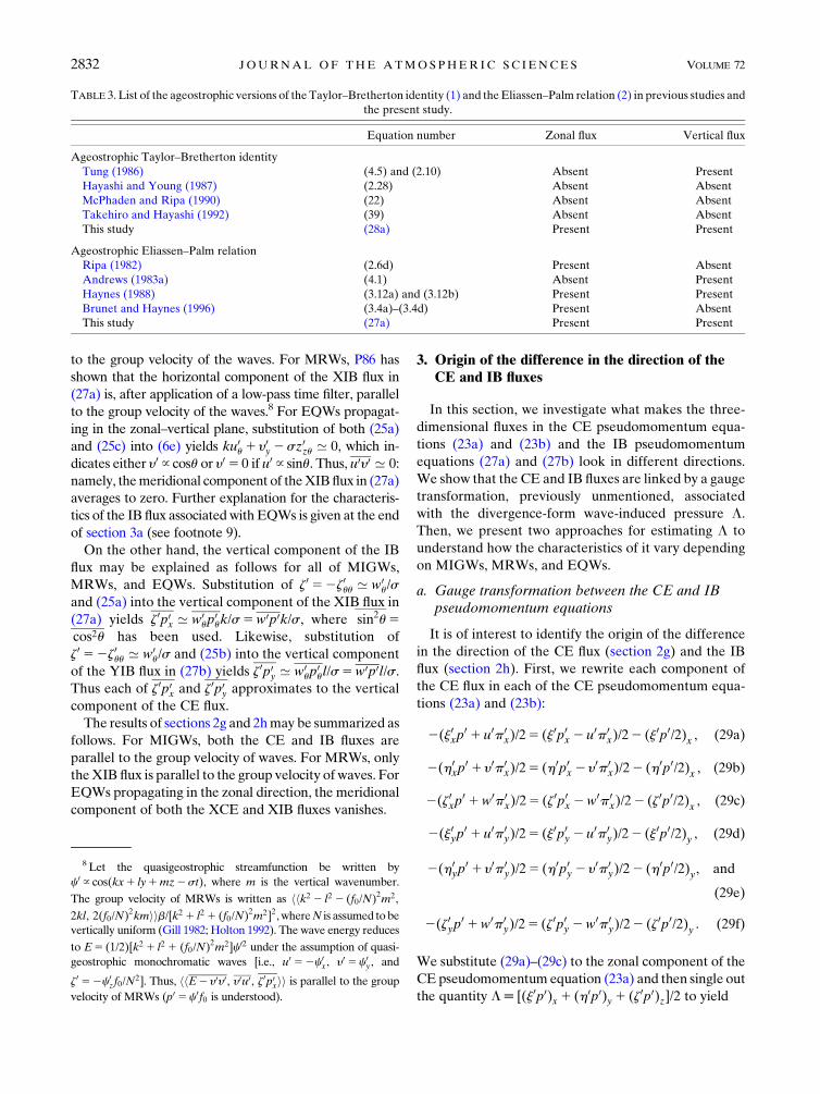
TABLE 3. List of the ageostrophic versions of the Taylor–Bretherton identity (1) and theEliassen–Palm relation (2) in previous studies and

the present study.

Equation number Zonal flux Vertical flux

Ageostrophic Taylor–Bretherton identity

Tung (1986) (4.5) and (2.10) Absent Present

Hayashi and Young (1987) (2.28) Absent Absent

McPhaden and Ripa (1990) (22) Absent Absent

Takehiro and Hayashi (1992) (39) Absent Absent

This study (28a) Present Present

Ageostrophic Eliassen–Palm relation

Ripa (1982) (2.6d) Present Absent

Andrews (1983a) (4.1) Absent Present

Haynes (1988) (3.12a) and (3.12b) Present Present

Brunet and Haynes (1996) (3.4a)–(3.4d) Present Absent

This study (27a) Present Present

8 Let the quasigeostrophic streamfunction be written by

c0 } cos(kx1 ly1mz2st), where m is the vertical wavenumber.

The group velocity of MRWs is written as hhk2 2 l2 2 (f0/N)2m2,

2kl, 2(f0/N)2kmiib/[k2 1 l2 1 (f0/N)2m2]2, whereN is assumed to be

vertically uniform (Gill 1982; Holton 1992). The wave energy reduces

to E5 (1/2)[k2 1 l2 1 (f0/N)2m2]c02 under the assumption of quasi-

geostrophic monochromatic waves [i.e., u0 52c0x, y0 5c0

y, and

z0 52c0zf0/N

2]. Thus, hhE2 y0y0, y0u0, z0p0xii is parallel to the group

velocity of MRWs (p0 5c0f0 is understood).


[(2u0j0x2 y0h0x1 z0p0

zx)/2|fflfflfflfflfflfflfflfflfflfflfflfflfflfflfflfflfflfflfflfflffl{zfflfflfflfflfflfflfflfflfflfflfflfflfflfflfflfflfflfflfflfflffl}CE pseudomomentum

]t 52$ � hh(j0p0x2 u0p0x)/22L, (h0p0x 2 y0p0

x)/2, (z0p0x2w0p0

x)/2ii , (30a)

where the direction of the three-dimensional flux (which

appears inside the divergence operator) has been

changed from that in (23a), although the divergence of

the flux remains the same. Likewise, we substitute (29d)–

(29f) to the meridional component of the CE pseudo-

momentum equation (23b) and then single out L to yield

[(2u0j0y2 y0h0y1 z0p0

zy)/2|fflfflfflfflfflfflfflfflfflfflfflfflfflfflfflfflfflfflfflfflffl{zfflfflfflfflfflfflfflfflfflfflfflfflfflfflfflfflfflfflfflfflffl}CE pseudomomentum

]t 52$ � hh(j0p0y2 u0p0y)/2, (h

0p0y2 y0p0y)/22L, (z0p0y2w0p0

y)/2ii1b(y0j02 u0h0) , (30b)

where the direction of the three-dimensional flux (which

appears inside the divergence operator) has been

changed from that in (23b), although, as before, the di-

vergence of the flux remains the same.

Below we show that the modified forms of the CE

pseudomomentum equations (30a) and (30b) are closely

related with the IB pseudomomentum (27a) and (27b).

First, we multiply (6a), (6b), and (9) by j0, h0, and N2z0,respectively, and then take the sum of the three equa-

tions to yield

(j0u0t 1h0y0t)2 f (j0y02h0u0)

1 j0p0x1h0p0y1 z0p0z1N2z02 5 0. (31)

Equation (31) may be written as

L52E1 (u0u0 2 j0u0t 1 y0y02h0y0t)/21 f (j0y0 2h0u0)/2,(32)

where E[ (u02 1 y02 1N2z02)/2 should be understood.

Using (32), we now investigate each component of

the three-dimensional flux in the modified forms

of the CE pseudomomentum equations (30a) and

(30b):

(j0p0x2 u0p0x)/22L5E2 y0y01 (y0h0)t/2 , (33a)

(h0p0x2 y0p0x)/25 y0u0 2 (u0h0)t/2 , (33b)

(z0p0x2w0p0x)/25 z0p0x2 (z0p0

x)t/2 , (33c)

(j0p0y2 u0p0y)/25 u0y02 (y0j0)t/2 , (33d)

(h0p0y2 y0p0y)/22L5E2 u0u01 (u0j0)t/2, and (33e)

(z0p0y2w0p0y)/25 z0p0y2 (z0p0

y)t/2 , (33f)

where (33a) and (33e) have been derived using (6a) and

(6b), (16a) and (16b), and (32) (detailed derivation in

the supplemental material). We now substitute (33a)–

(33f) into the modified forms of the CE pseudomo-

mentum equations (30a) and (30b) to yield

½(2u0j0x 2 y0h0x1 z0p0

zx)/2|fflfflfflfflfflfflfflfflfflfflfflfflfflfflfflfflfflfflfflfflfflffl{zfflfflfflfflfflfflfflfflfflfflfflfflfflfflfflfflfflfflfflfflfflffl}CE pseudomomentum

�t 52$ � hhE2 y0y01 (y0h0)t/2, y0u02 (u0h0)t/2, z

0p0x2 (z0p0x)t/2ii and (34a)

½(2u0j0y2 y0h0y 1 z0p0

zy)/2|fflfflfflfflfflfflfflfflfflfflfflfflfflfflfflfflfflfflfflfflfflffl{zfflfflfflfflfflfflfflfflfflfflfflfflfflfflfflfflfflfflfflfflfflffl}CE pseudomomentum

�t 52$ � hhu0y0 2 (y0j0)t/2,E2 u0u01 (u0j0)t/2, z0p0y 2 (z0p0

y)t/2ii1b(y0j0 2 u0h0)/2.

(34b)

It is clear that moving all terms with time derivatives

on the right-hand sides of (34a) and (34b) to the left-

hand side will lead to reproduction of the IB pseudo-

momentum equations (27a) and (27b), understanding

the explicit relationship between the CE pseudomo-

mentum and the IB pseudomomentum in (18a) and

(18b). We conclude that the quantity L[ [(j0p0)x 1(h0p0)y 1 (z0p0)z]/2 is at the heart of the difference in

the direction of the CE and IB fluxes, which has been

little mentioned in previous studies. It can be said that

the IB and CE fluxes are linked by a gauge trans-

formation associated with L. The quantity L is also


useful for understanding the characteristics of the XIB

flux associated with EQWs propagating in the zonal-

vertical plane.9

In the rest of this section, we investigate the character-

istics of L for MIGWs, MRWs, and EQWs. In particular,

we suggest two approaches for estimating L. The first ap-

proach is based on the combination of the virial theorem

and the potential vorticity equation (section 3b). The

second approach is based on the assumption of nearly

plane waves in the horizontal direction (section 3c).

b. First approach to estimate L: The combination ofthe virial theorem and the potential vorticityequation

For readers who are unfamiliar with the virial theo-

rem, we begin with noting a well-known equipartition

statement between the wave kinetic energy K and the

wave potential energyG associated with linear waves in

a nonrotating frame (Bühler 2009). The equipartition

statement may be shown by manipulating (31) to yield

[(j0u0 1h0y0)/2]t 2 f (j0y02h0u0)/2

1 [(j0p0)x1 (h0p0)y 1 (z0p0)z]/2|fflfflfflfflfflfflfflfflfflfflfflfflfflfflfflfflfflfflfflfflfflfflfflfflfflffl{zfflfflfflfflfflfflfflfflfflfflfflfflfflfflfflfflfflfflfflfflfflfflfflfflfflffl}[L

1G5K . (35)

If steady waves in a periodic nonrotating domain are con-

sidered, the first three terms on the left-hand side of (35)

vanish after application of a low-pass time filter. The result

is that G becomes equal to K. Equation (35) may be re-

ferred to as an Eulerian expression for the virial theorem.

For waves in a rotating frame, Andrews andMcIntyre

(1978b, hereafter AM78b) have used the virial theorem

to explain the concept of generalized wave action.

AM78b have eventually focused on three-dimensionally

homogeneous waves (i.e., waves other than planetary

waves) to ignore L. This may be confirmed by noting

that 2L in the present study corresponds to (1/r)(jjp0),j

in (B2) of AM78b. Likewise, 2(L1G) in the present

study corresponds to (1/~r)jiKij(pj),j in (4.10) of AM78b.

On the other hand, Eckart (1963) has used the virial

theorem to consider the stability problem of a mean

flow. He has eventually removed L by taking a volume

integral.

We suggest that the virial theorem, as expressed by

(35), is actually applicable to all waves at all latitudes as

long as L is retained. Substitution of the potential vor-

ticity equation (11) and (25c) and (25d) into (35) and

then application of a low-pass time filter yields

L ’ K2G1 (f /b)q0u0 , (36)

which allows us to estimate L analytically and numeri-

cally. Because h0 52q0/b has been used, (36) is applica-

ble to bothEQWsandMRWs, but notMIGWs (Table 2).

It should be noted that (36) provides no restriction for

the vertical profile of waves, which enables, if necessary,

the buoyancy frequency to vary in the vertical direction.

Namely, it does not matter whether waves are nearly

plane or nonplane in the vertical direction. For EQWs

(which have a trappedmodal structure in the meridional

direction), one may easily expect that (h0p0)y 6¼ 0 and

thus anticipate that L is nonzero. On the other hand, for

MRWs, L must be nonzero in order for the CE and IB

fluxes to look in different directions, but this is not ob-

vious from (36). To summarize, while (36) will be useful

for the model diagnosis of L in a future study, it is not so

useful for interpreting L.

c. Second approach to estimate L: The assumption ofnearly plane waves in the horizontal direction

We develop another equation to diagnose L:

L5 (j0p0x1h0p0y 1 z0p0z)/2

5 (j0p0x1h0p0y)/22 (N2/2)z02

5 [2(p0y 1 y0)p0x 1 (p0

x1 u0)p0y]/(2f )2 (N2/2)z02

5 [2p0yp

0x1p0

xp0y]/(2f )

1 [y0(2p0x 1 f y0)1 u0(p0y1 fu0)]/(2f )2E , (37)

where the first line has been derived using (8), the sec-

ond line has been derived using (9), the third line has

been derived using (16a) and (16b), and the last line has

been derived using E[ (u02 1 y02 1N2z02)/2. It shouldbe noted that (37) provides no restriction for the vertical

profile of waves, which enables, if necessary, the buoy-

ancy frequency N to vary in the vertical direction.

Namely, it does not matter whether waves are nearly

plane or nonplane in the vertical direction.

9 Substitution of (33a) to the zonal component of the XIB flux in

(27a) yields E2 y0y0 52L1 (j0p0x 2u0p0x)/22 (h0y0)t 52(j0xp

0 1u0p0

x)/22 [(h0p0)y 1 (z0p0)z 1 (h0y0)t]/2, where the 2(j0xp0 1u0p0

x)/2

part is identical to the zonal component of the XCE flux in

(23a) and thus approximates to u0p0k/s, as in (26a). The time

average of the remaining part [(h0p0)y 1 (z0p0)z 1 (h0y0)t]/2 ’[(h0p0)y 1 (z0p0)z]/2 vanishes after taking an areal integral in the

meridional–vertical plane, assuming meridionally and vertically

trapped waves. To summarize, for EQWs propagating in the

zonal–vertical plane, an areal integral in the meridional and

vertical section is understood when discussing the relationship

between the XIB flux and the group velocity of the waves, via the

pressure flux in the wave energy equation (14). This feature

originates from (18a), where the difference between the CE

pseudomomentum and the IB pseudomomentum is defined as

a flux divergence form.


An expression for L that is suitable for analytical in-

terpretation may be obtained by substituting (6a) and

(6b) into the right-hand side of (37) and then applying

a low-pass time filter to yield

L5 (2p0yp

0x1p0

xp0y)/(2f )|fflfflfflfflfflfflfflfflfflfflfflfflfflfflfflfflfflffl{zfflfflfflfflfflfflfflfflfflfflfflfflfflfflfflfflfflffl}

’0 for plane waves

1 (u0ty02 u0y0t)/(2f )

zfflfflfflfflfflfflfflfflfflfflfflfflffl}|fflfflfflfflfflfflfflfflfflfflfflfflffl{’E for MIGWs

|fflfflfflfflfflfflfflfflfflfflfflfflfflffl{zfflfflfflfflfflfflfflfflfflfflfflfflfflffl}’0 for MRWs

2E .

(38)

The first term on the right-hand side of (38) vanishes for

both MIGWs and MRWs (but it is nonzero for EQWs, as

will be explained later in the next paragraph). This is be-

cause the assumption of nearly plane waves allows (25a)–

(25d) to be used to yield (2p0yp

0x 1p0

xp0y)/(2f ) ’

(p0up

0uu 2p0

up0uu)kls/(2f )5 0. The characteristics of

the second term on the right-hand side of (38) vary

depending on MIGWs and MRWs. For MIGWs,

substitution of a standard analytical solution for three-

dimensional plane waves (wherein N is assumed to be

a vertically uniform constant; see appendix A) to

the term leads to (u0ty 0 2u0y0t)/(2f ) ’ E. On the other

hand, for MRWs, (u0ty0 2 u0y 0t)/(2f ) ’ (2p0ytp0x 1 p0yp0xt)/(2f 2) ’ (p0uup

0u 2p0up

0uu)kls/(2f

2)5 0, where both geo-

strophic velocity and (25a)–(25d) have been used. To

summarize, (38) yields L ’ 0 for MIGWs and L ’ 2E

for MRWs (Table 2). In section 3a, we have explained

that L is at the heart of the difference in the direction of

the CE flux in (23a) and (23b) and the IB flux in (27a)

and (27b), referencing (30) and (33a)–(33f). That L ’ 0

for MIGWs (at least for uniform N) is surely important

and worth emphasizing. This is why the CE flux in (23a)

and (23b) and the IB flux in (27a) and (27b) both are

parallel to the direction of the group velocity for

MIGWs. That L is nonzero for MRWs means that these

two fluxes point in different directions in that case, and

since the IB flux in (27a) is parallel to the direction of the

group velocity forMRWs (see footnote 8), theCE flux in

(23a) cannot be.

On the other hand, for EQWs, the characteristics of

both the first and second terms on the right-hand side of

(38) are unclear. Nevertheless, for EQWs (and MRWs),

we have already explained that (36) may be used. See

also footnote 9. The above-mentioned approaches [i.e.,

the set of (36) and (37)] to estimate L are complemen-

tary to each other and have been developed for the

understanding of the difference in the direction of the

CE and IB fluxes. The two approaches are also useful,

via the virial theorem (35), for the estimation of the

quantity (j0y0 2h0u0)/2 ’ j0y0 ’ 2h0u0 associated with

the Stokes-drift velocity in (12a) and (12b) (appendix B

and Table 2).

To summarize this section, we have investigated what

makes the CE and IB fluxes look in different directions.

Since the CE and IB pseudomomenta only differ by

divergence of a vector [see (18a) and (18b)], their

prognostic equations are related through the gauge

transformation associated with the divergence-form

wave-induced pressure L, which is the most important

result of the present study (section 3a). Then we have

investigated the characteristics of L for MIGWs,

MRWs, and EQWs, with two approaches for estimating

L. The first approach is based on the combination of the

virial theorem and the potential vorticity equation and is

applicable to MRWs and EQWs (section 3b). The sec-

ond approach is based on the assumption of nearly plane

waves in the horizontal direction and is applicable to

MIGWs and MRWs (section 3c).

One of the reasons why we have used the CE flux as

a reference for affirming the direction of the IB flux is

that the CE flux is proportional to not only the pressure

flux in the wave energy equation, but also the three-

dimensional form stress in the three-dimensional LM

momentum equations (see section 4a). Namely, the

three-dimensional form stress is parallel to the direction

of the group velocity of MIGWs, but not for MRWs, as

explained in the next section.

4. The effect of waves on the mean flow

Using analytical solutions for MIGWs and MRWs,

M06 and Kinoshita and Sato (2013, hereafter KS13)

have derived three-dimensional versions of the TEM

momentum equation (3) and then examined whether

the wave-inducedmomentumflux on the right-hand side

of their TEM momentum equations is parallel to the

group velocity of waves. In both studies, the Coriolis

term of their TEM momentum equations has been

written in terms of the LM velocity: namely, the sum of

the EM velocity and the Stokes-drift velocity [see (12a)

and (12b)]. Noda (2010) has shown, in a general way,

a basis for writing the Coriolis term using the LM ve-

locity, which is revisited in section 4a as a preliminary

discussion for this section.

In section 4b, we derive a generalized version of the

TEM momentum equation (3), in which the effect of

waves on the mean flow is found to be represented

by the set of the Coriolis–Stokes force, the three-

dimensional divergence of the IB flux, and the hori-

zontal gradient of L. This indicates another utility of Lthat has been little mentioned in previous studies. In

section 4c, we derive a generalized version of theMEM

momentum equation (4), in which the prognostic

quantity is found to be the sum of the EM velocity and

the DI wave activity in (20a) and (20b). All equations in


sections 4b and 4c are applicable to MIGWs, MRWs,

and EQWs.

a. Low-pass-filtered momentum equations based onthe three-dimensional form stress

In the standard EM momentum equations (5a)

and (5b), the effect of waves on the mean flow has

been represented by the three-dimensional Reynolds

stress, which we wish to transform using (6a), (6b),

and (7):

u0u0 5 (j0u0)t 2 j0u0t 5 (j0u0)t 1 j0p0x 2 f j0y0 , (39a)

y0u0 5 (h0u0)t 2h0u0t 5 (h0u0)t 1h0p0x2 fh0y0 , (39b)

w0u0 5 (z0u0)t 2 z0u0t 5 (z0u0)t 1 z0p0x2 f z0y0 , (39c)

u0y05 (j0y0)t 2 j0y0t 5 (j0y0)t 1 j0p0y1 f j0u0 , (39d)

y0y05 (h0y0)t 2h0y0t 5 (h0y0)t 1h0p0y1 fh0u0, and

(39e)

w0y0 5 (z0y0)t 2 z0y0t 5 (z0y0)t 1 z0p0y1 f z0u0 . (39f)

Substitution of (39a)–(39f) to the standard EM mo-

mentum equations (5a) and (5b) yields (Fig. 2)

(u1 uStokes)t 1$ � (U u)2 f (y1 yStokes)2b(h0y0)

52px2$ � hhj0p0x,h0p0x, z0p0xii and

(40a)

(y1 yStokes)t 1$ � (U y)1 f (u1 uStokes)1b(h0u0)

52py2$ � hhj0p0y,h0p0y, z0p0yii ,

(40b)

where the last terms of each of (40a) and (40b) represents

the divergence of three-dimensional form stress (i.e., the

residual effect of pressure perturbations). Both the Cori-

olis term and the tendency term of (40a) and (40b) have

been written in terms of the sum of the EM velocity and

the Stokes-drift velocity: namely, the LM velocity. The

Coriolis term of (40a) and (40b) may be interpreted as

2f (y1 yStokes)2b(h0y0)

52f y2 (j0f y 0)x2 (h0f y0)y 2 (z0f y0)z and

(41a)

1 f (u1 uStokes)1b(h0u0)

51fu1 (j0fu0)x1 (h0fu0)y1 (z0fu0)z. (41b)

FIG. 2. Relationship of the seven sets of low-pass time-filtered momentum equations in

the present study: SEM is the standard EM momentum equations (5a) and (5b), DLM is

(an Eulerian approximation for) the direct expression of the three-dimensional LM mo-

mentum equations (40a) and (40b), WIM is (an Eulerian approximation for) the thickness-

weighted isopycnal-mean momentum equations (43a) and (43b), TEM is the generalized

transformed EM momentum equations (44a) and (44b), MEM is the merged form of the

EM momentum equations (45a) and (45b), UIM is (an Eulerian approximation for) the

unweighted isopycnal-mean momentum equations (46a) and (46b) in a vector-invariant

form, and TLM is (an Eulerian approximation for) the transformed expression of the

three-dimensional LM momentum equations (51a) and (51b). The set of TEM and MEM

originates from the Eliassen–Palm theory, as noted by thick boxes. The set of WIM and

UIM originates from the isopycnal-mean theory. The set of DLM and TLM originates from

the generalized LM theory. The quantity L is found in each of the TEM, MEM, and TLM

momentum equations.


Thus, the set of (40a) and (40b), combined with

(41a) and (41b), represents an Eulerian approximation

for the three-dimensional LM momentum equations.10

In the rest of this subsection, we specialize for, as

in section 2g, waves that are nearly plane in the hor-

izontal direction (such as MIGWs or MRWs; see

Table 2). Using (25a)–(25d), we rewrite each com-

ponent of the three-dimensional form stress in (40a)

and (40b) as

j0p0x ’ u0up0uk/s5 u0p0k/s , (42a)

h0p0x ’ y0up0uk/s5 y0p0k/s , (42b)

z0p0x ’ w0up

0uk/s5w0p0k/s , (42c)

j0p0y ’ u0up0ul/s5 u0p0l/s , (42d)

h0p0y ’ y0up0ul/s5 y0p0l/s, and (42e)

z0p0y ’ w0up

0ul/s5w0p0l/s , (42f)

where both hhj0, h0, z0ii5 hh2j0uu, 2h0uu, 2z0uuii ’ hhu0u,

y0u, w0uii/s and (sinu)2 5 (cosu)2 have been used. The set

of (42a)–(42f) allows us to interpret the three-dimensional

form stress in (40a) and (40b) as the CE flux in (26a) and

(26b), which has already been suggested, for example, in

(20) of Noda (2010).

To summarize, replacing the EM velocity in the

Coriolis term of (5a) and (5b) with the LM velocity

leads to two consequences. First, the Reynolds stress in

(5a) and (5b) is replaced by the form stress, as in (40a)

and (40b). Second, the tendency term of (40a) and

(40b) is written in terms of the LM velocity. Both

consequences are implicit in M06 and KS13, who have

used analytical solutions for waves (where wave

amplitude, wavenumber, and wave frequency are

practically constant; see footnote 4).

The CE flux in (42a)–(42f) is proportional to the

pressure flux hhu0p0, y0p0, w0p0ii in (14), and thus is not,

after application of a low-pass filter, parallel to the group

velocity of MRWs (sections 2d and 2g). Moreover s/k

and s/l in (42a)–(42f) are not readily available from

model output. For these reasons, the Eulerian approxi-

mation for the LM momentum equations (40a) and

(40b) with the three-dimensional form stress are not

used in the rest of this paper. Likewise, the CE pseu-

domomentum equations (23a) and (23b) are not used in

the rest of this paper.

b. Low-pass-filtered momentum equations based onthe IB flux

We shall seek a more useful expression for low-pass

time-filteredmomentumequations concerning the effect of

waves on themeanflow.Asmentioned in section 2h, the IB

pseudomomentum vector is useful because (i) the XIB flux

in (27a) is parallel to the group velocity of MRWs, (ii) the

XIB andYIB fluxes in (27a) and (27b) are in an expression

that is suitable for model diagnosis (i.e., k, l,s, j0, and h0

are absent), (iii) it does not matter whether waves are

nearly plane or nonplane in the horizontal direction, and

(iv) there is a clear relationship [(20a) and (20b)] between

the IB pseudomomentum vector and the DI wave activity.

All equations shown below are applicable to the various

types of linear hydrostatic neutral waves in a planetary

fluid, such as MIGWs, MRWs, and EQWs.

Substitution of only the vertical component of the

Reynolds stress (39c) and (39f) to the standard EM

momentum equations (5a) and (5b) yields (Fig. 2)

(u1uqs)t 1$ � (U u)2 f (y1 yqs)

52px 2$ � hhu0u0, y0u0, z0p0xii52(p2G1K)x2$ � hhE2 y0y0, y0u0, z0p0xii and

(43a)

(y1 yqs)t 1$ � (U y)1 f (u1 uqs)

52py 2$ � hhu0y0, y0y0, z0p0yii52(p2G1K)y2$ � hhu0y0,E2u0u0, z0p0yii , (43b)

where the last line of each of (43a) and (43b) has been

written in such a way as to single out the three-

dimensional divergence of the IB flux in each of (27a)

and (27b), respectively. It should be noted that the

tendency term as well as the Coriolis term of (43a) and

(43b) has been written in terms of the sum of the EM

velocity and the quasi-Stokes velocity. Thus, the set of

(43a) and (43b) represents an Eulerian approximation

10 The tendency, Coriolis, and pressure gradient terms of (40a)

and (40b) consist of quantities that may be written using the same

operatorA1 (j0A0)x 1 (h0A0)y 1 (z0A0)z forA5 u, y, px, py, fy, and

fu (i.e., an Eulerian approximation for the LM operator). Note that

only the linear terms (i.e., the tendency, Coriolis, and pressure

gradient terms) of the standard EMmomentum equations (5a) and

(5b) may be expressed using this operator in (40a) and (40b). The

mean-flow advection term of (40a) and (40b) is out of the effect of

this operator. This is because both sufficiently weakmean flows and

small-amplitude linear waves have been assumed in the present

study. The set of (40a) and (40b) is closely related to a type of LM

momentum equation in the previous literature that has been

written for the development of the LM velocity (not to be confused

with another type of LM momentum equation that is written for

the development of the LM velocity minus the GL pseudomo-

mentum vector). See AM78a and AG14 (see their Table 1) for

details. A related explanation appears in footnote 14.


for the thickness-weighted isopycnal-mean momentum

equations.11

The first term on the right-hand sides of (43a)

and (43b) contains the quantity 2G1K, which is

the wave kinetic energy minus the wave potential

energy. To manipulate this quantity, we substitute the

virial theorem (35) into (43a) and (43b) to yield

(Fig. 2)

[u1 uqs 1 (j0u01h0y0|fflfflfflfflfflffl{zfflfflfflfflfflffl}’0

) x/2]t 1$ � (Uu)2 f [y1 yqs 1 (j0y0 2h0u0)x/2]

52(p1L)x2$ � hhE2 y0y0, y0u0, z0p0xii and (44a)

[y1 yqs 1 (j0u0 1h0y0|fflfflfflfflfflffl{zfflfflfflfflfflffl}’0

) y/2]t 1$ � (U y)1 f [u1 uqs 2 (j0y02h0u0)y/2]1b(h0u02 j0y0)/2

52(p1L)y2$ � hhu0y0,E2 u0u0, z0p0yii , (44b)

where the quantity j0u0 1h0y0 in the tendency term of

each equation averages to zero because of the phase

relationship of neutral waves satisfying the WKB

approximation. Nevertheless, this term shall be kept

in what follows (thus, all equations in this section are

written using an equal sign), since retaining this term

will prove useful in a future study for nonneutral

waves.

Equations (44a) and (44b) represent a skeleton model

for the generalized TEMmomentum equations that have

been targeted in the atmospheric literature. Indeed, the

sum of the EM velocity and the quasi-Stokes velocity,

y1 yqs, in the Coriolis term of (44a) corresponds to the

velocity y*5 ya 1 (2ryyy /rz)z in the classical TEM

momentum equation (3). Likewise, the meridional and

vertical components of the XIB flux in (44a) correspond

to hhFy, Fzii in the classical TEM momentum equation

(3). The set of (44a) and (44b) represents a unified

expression for the effect of the various types of linear

hydrostatic neutral waves in a planetary fluid, such as

MIGWs, MRWs, and EQWs, on mean flows. As in (43a)

and (43b), the last term on the right-hand sides of (44a)

and (44b) represents the divergence of the IB flux in

(27a) and (27b). Substitution of L ’ 0 and L ’ 2E (asso-

ciated withMIGWs andMRWs, respectively; see section 3c

and Table 2) to the generalized TEMmomentum equations

(44a) and (44b) yields an equation system that is consistent

with the systems of M06 and TN01, respectively.12

c. Low-pass-filtered momentum equations based onthe tendency of the DI wave activity

Subtraction of the IB pseudomomentum equations

(27a) and (27b) from the generalized TEM momentum

equations (44a) and (44b) yields (Fig. 2)


and (43b) consist of quantities that may be written using the same

operator A1 (z0A0)z for A5u, y, px, and py (i.e., an Eulerian ap-

proximation for the thickness-weighted-mean operator). Note that

only the linear terms (i.e., the tendency, Coriolis, and pressure

gradient terms) of the standard EMmomentum (5a) and (5b) may

be expressed using this operator in (43a) and (43b). The mean-flow

advection term and the horizontal Reynolds stress term (see the

second line of each equation) of (43a) and (43b) are out of the

effect of this operator. This is because both sufficiently weak mean

flows and small-amplitude linear waves have been assumed in the

present study. The set of (43a) and (43b) is closely related with the

mass-weighted isentropic-mean momentum equations in Andrews

(1983a), Bleck (1985), Tung (1986), and Iwasaki (1989, 2001), as

well as the thickness-weighted isopycnal-mean momentum equa-

tions in Greatbatch and McDougall (2003), Jacobson and Aiki

(2006), Aiki and Richards (2008), and Young (2012).

12 In the limit of a sufficiently weak mean flow, the quasigeo-

strophic wave activity flux associated with MRWs (that has been

symbolized by W) in TN01 corresponds to minus the XIB flux

hhE2 y0y0, y0u0, z0p0xii in the present study. Likewise, in the limit of

a sufficiently weak mean flow, another flux Ws 52CUM1W in

TN01 (where CU is the apparent phase velocity and M is their

quasigeostrophic wave activity associated with MRWs) corre-

sponds to minus the combined wave-induced momentum flux

hhL1E2 y0y0, y0u0, z0p0xii on the right-hand side of the generalizedTEM momentum equation in (44a) of the present study. See also

(8), (31), and (45)–(51) of TN01. This indicates that L in (44a) and

(44b) of the present study is closely related with CUM in TN01 in

the limit of a sufficiently weak mean flow. Indeed, after application

of an Eulerian time average (and also in the limit of a sufficiently

weak mean flow), M in (26) of TN01 reduces to

M ’ E/(jUj2Cp) ’ 2E/Cp, where the symbols U and Cp are

adapted from TN01. Thus, CUM ’ 2ECU /Cp 52EU/jUj, whichcorresponds to hhL, 0, 0ii ’ hh2E, 0, 0ii in the present study.


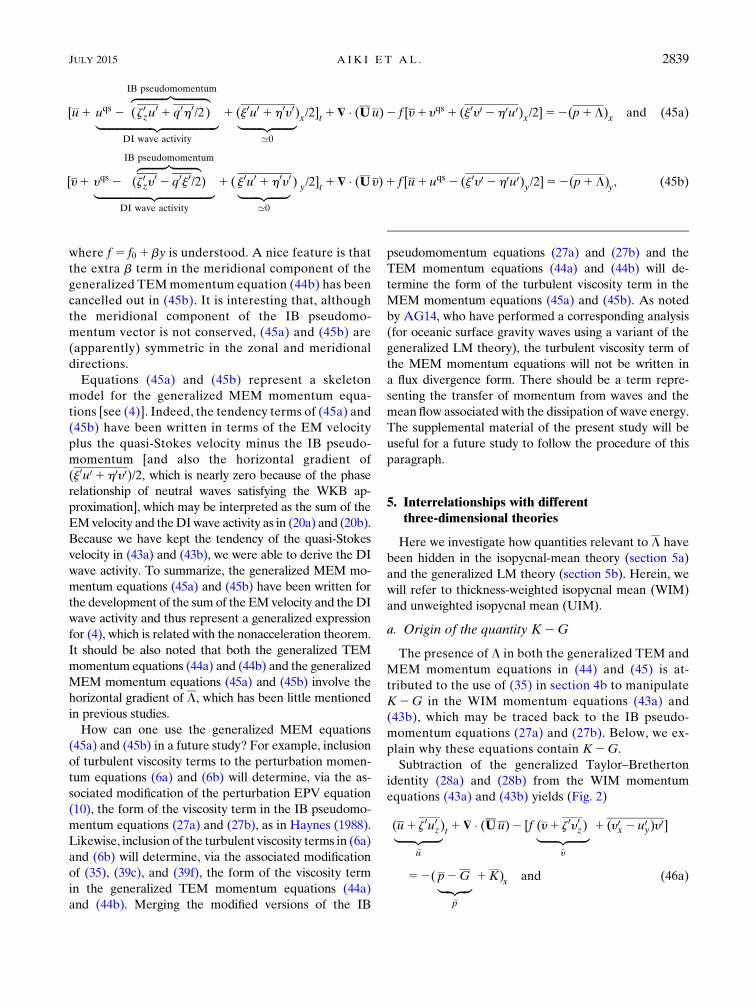
[u1 uqs 2 (z0zu01 q0h0/2)

zfflfflfflfflfflfflfflfflfflfflffl}|fflfflfflfflfflfflfflfflfflfflffl{IB pseudomomentum

|fflfflfflfflfflfflfflfflfflfflfflfflfflfflfflfflfflfflfflffl{zfflfflfflfflfflfflfflfflfflfflfflfflfflfflfflfflfflfflfflffl}DI wave activity

1 (j0u01h0y0)|fflfflfflfflfflfflffl{zfflfflfflfflfflfflffl}’0

x/2]t 1$ � (U u)2 f [y1 yqs 1 (j0y02h0u0)x/2]52(p1L)x and (45a)

[y1 yqs 2 (z0zy02 q0j0/2

zfflfflfflfflfflfflfflffl}|fflfflfflfflfflfflfflffl{)

IB pseudomomentum

|fflfflfflfflfflfflfflfflfflfflfflfflfflfflfflfflfflfflffl{zfflfflfflfflfflfflfflfflfflfflfflfflfflfflfflfflfflfflffl}DI wave activity

1 ( j0u01h0y0|fflfflfflfflfflffl{zfflfflfflfflfflffl}’0

) y/2]t 1$ � (U y)1 f [u1 uqs 2 (j0y0 2h0u0)y/2]52(p1L)y, (45b)

where f 5 f0 1by is understood. A nice feature is that

the extra b term in the meridional component of the

generalized TEMmomentum equation (44b) has been

cancelled out in (45b). It is interesting that, although

the meridional component of the IB pseudomo-

mentum vector is not conserved, (45a) and (45b) are

(apparently) symmetric in the zonal and meridional

directions.

Equations (45a) and (45b) represent a skeleton

model for the generalized MEM momentum equa-

tions [see (4)]. Indeed, the tendency terms of (45a) and

(45b) have been written in terms of the EM velocity

plus the quasi-Stokes velocity minus the IB pseudo-

momentum [and also the horizontal gradient of

(j0u0 1h0y0)/2, which is nearly zero because of the phase

relationship of neutral waves satisfying the WKB ap-

proximation], which may be interpreted as the sum of the

EMvelocity and theDIwave activity as in (20a) and (20b).

Because we have kept the tendency of the quasi-Stokes

velocity in (43a) and (43b), we were able to derive the DI

wave activity. To summarize, the generalized MEM mo-

mentum equations (45a) and (45b) have been written for

the development of the sum of the EMvelocity and theDI

wave activity and thus represent a generalized expression

for (4), which is related with the nonacceleration theorem.

It should be also noted that both the generalized TEM

momentum equations (44a) and (44b) and the generalized

MEM momentum equations (45a) and (45b) involve the

horizontal gradient of L, which has been little mentioned

in previous studies.

How can one use the generalized MEM equations

(45a) and (45b) in a future study? For example, inclusion

of turbulent viscosity terms to the perturbation momen-

tum equations (6a) and (6b) will determine, via the as-

sociated modification of the perturbation EPV equation

(10), the form of the viscosity term in the IB pseudomo-

mentum equations (27a) and (27b), as in Haynes (1988).

Likewise, inclusion of the turbulent viscosity terms in (6a)

and (6b) will determine, via the associated modification

of (35), (39c), and (39f), the form of the viscosity term

in the generalized TEM momentum equations (44a)

and (44b). Merging the modified versions of the IB

pseudomomentum equations (27a) and (27b) and the

TEM momentum equations (44a) and (44b) will de-

termine the form of the turbulent viscosity term in the

MEM momentum equations (45a) and (45b). As noted

by AG14, who have performed a corresponding analysis

(for oceanic surface gravity waves using a variant of the

generalized LM theory), the turbulent viscosity term of

the MEM momentum equations will not be written in

a flux divergence form. There should be a term repre-

senting the transfer of momentum from waves and the

mean flow associated with the dissipation of wave energy.

The supplemental material of the present study will be

useful for a future study to follow the procedure of this

paragraph.

5. Interrelationships with differentthree-dimensional theories

Here we investigate how quantities relevant to L have

been hidden in the isopycnal-mean theory (section 5a)

and the generalized LM theory (section 5b). Herein, we

will refer to thickness-weighted isopycnal mean (WIM)

and unweighted isopycnal mean (UIM).

a. Origin of the quantity K2G

The presence of L in both the generalized TEM and

MEM momentum equations in (44) and (45) is at-

tributed to the use of (35) in section 4b to manipulate

K2G in the WIM momentum equations (43a) and

(43b), which may be traced back to the IB pseudo-

momentum equations (27a) and (27b). Below, we ex-

plain why these equations contain K2G.

Subtraction of the generalized Taylor–Bretherton

identity (28a) and (28b) from the WIM momentum

equations (43a) and (43b) yields (Fig. 2)

(u1 z0u0z)|fflfflfflfflffl{zfflfflfflfflffl}~u

t 1$ � (Uu)2 [f (y1 z0y0z)|fflfflfflfflfflffl{zfflfflfflfflfflffl}~y

1 (y0x2 u0y)y0]

52( p2G|fflfflffl{zfflfflffl}~p

1K)x and (46a)


( y1 z0y0z|fflfflfflffl{zfflfflfflffl}~y

) t 1$ � (U y)1 [f (u1 z0u0z)|fflfflfflfflfflfflffl{zfflfflfflfflfflfflffl}~u

1 (y0x2 u0y)u0]

52( p2G|fflfflffl{zfflfflffl}~p

1K)y , (46b)

which has been derived using q0 5 y0x 2 u0y 2 f z0z. Equa-tion (46a) contains 2(y0x 2 u0y)y0 on the left-hand side

and 2Kx on the right-hand side, which is a vector-

invariant form of the horizontal advection term

u0u0x 1 y0u0y. Likewise, (46b) contains 1(y0x 2 u0y)u0 on theleft-hand side and 2Ky on the right-hand side, which is

a vector-invariant form of the horizontal advection term

u0y0x 1 y0y0y. This explains whyK has the same status as p.

However, it is still unclear why the sign in front of G is

negative in (46a) and (46b), a topic we shall discuss in

what follows.

We seek to understand the tendency, the Coriolis, and

the pressure gradient terms of (46a) and (46b) using an

approximate expression for the UIM (denoted by the

tilde) of an arbitrary quantity A, as follows:

~A[A1 z0Az1 (z02/2)Azz 1⋯

5A1 z0A0z1 (z02/2)Azz 1⋯ , (47)

which has been written up to the second order in terms

of a Taylor expansion in the vertical direction; the

second line omits the triple and higher product of

perturbation quantities. The right-hand side of (47) has

been written in terms of quantities averaged in Euler-

ian coordinates. Equation (47) allows us to interpret

both the tendency term and the Coriolis term of (46a)

and (46b) in terms of ~u and ~y. An exception is that the

second-order derivative term on the last line of (47)

(viz., Azz 5 uzz and yzz) is absent in (46a) and (46b).

This is because the IB pseudomomentum equations

(27a) and (27b), as well as the generalized Taylor–

Bretherton identity (28a) and (28b), have been derived

from the equation system (6a)–(11) for linear waves

with no mean flow. On the other hand, substitution of

A 5 p to (47) yields

~p5 p1 z0p0z1 (z02/2)pzz1⋯

5 p2 z02N21 (z02/2)N21⋯

5 p2 (z02/2)N2|fflfflfflfflfflffl{zfflfflfflfflfflffl}G

1⋯ , (48)

where both (9) and N2 [2rzg/r0 (i.e., hydrostatic re-

lation for the wave and mean fields, respectively) have

been used to derive the second line, and the last line

indicates that the EM pressure p is always greater than

the UIM pressure ~p on the left-hand side. The differ-

ence between p and ~p is illustrated in Fig. 3, where the

density of fluid particles in regions A–F increases in an

alphabetical order. The EM pressure partially in-

cludes particles in the region D (of greater density)

and also partially excludes particles in the region C (of

smaller density). The gain of mass for p from the re-

gion D is greater than the loss of mass for p from the

region C, which indicates that p is always greater than

~p compared at a given reference height and is consis-

tent with (48). The above interpretation is also con-

sistent with a generalized expression for the wave

potential energy:Ð z1z0z r dzg/r0, as given by Holliday

and McIntyre (1981).

FIG. 3. A time series for the vertical profile of density in a con-

tinuously stratified fluid (contour). The shading shows the area of

density that is used to calculate (a) the Eulerian-mean hydrostatic

pressure and (b) the isopycnal-mean hydrostatic pressure. The

density of fluid particles in regions A–F increases in an alpha-

betical order. Fluid particles in region D are counted in the Eu-

lerian-mean pressure but not the isopycnal-mean pressure, which

explains why the Eulerian-mean pressure is always greater than

the isopycnal-mean pressure compared at the same reference

height.


Substitution of A5 px into (47) yields g(px)5 (px)1z0p0xz 5 (px)2 z0z0xN

2 5 ›x(p2G)5 ›x(~p), where both

the subscript x and the symbol ›x refer to the same

zonal gradient operator at fixed height. Namely, con-

cerning the treatment of hydrostatic pressure, the

UIM operator and the fixed-height zonal gradient

operator commute. This can be also confirmed with-

out using the Taylor expansion in (47) but using den-

sity coordinates (to be explained in detail in our future

study). The result is that the pressure gradient term of

(46a) may be interpreted as ›x(p2G)5 ›x(~p)5 g(px).The same analysis holds for the pressure gradient term

in (46b). Thus, the set of (46a) and (46b) represents an

Eulerian approximation for the UIM momentum

equations in a vector-invariant form.13 This explains

why the sign in front ofG in (46a) and (46b) is opposite

to the sign in front of K. To summarize, the general-

ized Taylor–Bretherton identity (28a) and (28b) may

be interpreted as the difference of the WIM momen-

tum equations (43a) and (43b) and the UIM momen-

tum equations (46a) and (46b) in a vector-invariant

form. This explains the origin of 2K1G in (28a) and

(28b) and thus in the IB pseudomomentum equations

(27a) and (27b).

Additional results may be obtained if the UIM ve-

locity is interpreted as the sum of the EM velocity and

the gravity wave part of the DI wave-activity vector in

(20a) and (20b): hh~u, ~yii5 hhu1 z0u0z, y1 z0y0zii. Thisindicates that the UIM momentum equations (46a)

and (46b) are closely related with the MEM mo-

mentum equations (45a) and (45b), concerning the

treatment of hydrostatic gravity waves. Without the

above recognitions (one is associated with the Tay-

lor–Bretherton identity, mentioned in the previous

paragraph, and one is associated with the gravity

wave part of the wave activity, mentioned in the

present paragraph), previous studies have not paid

a significant attention to the UIM momentum equa-

tions (46a) and (46b), except for Tung (1986) and

Greatbatch (1998). Probably the UIM velocity has

been thought not to be a robust quantity because its

volume integral does not become identical to that of

the EM velocity. It is the WIM velocity for which the

volume integral becomes identical to that of the EM

velocity [see the pileup rule in Aiki and Yamagata

(2006)]. See also Fig. 2 to note that what is missing in

both WIM and UIM is the virial theorem (35), which

is why L is absent in the WIM and UIM momentum

equations.

b. Prototype of the quantity p1L

The right-hand side of the MEM momentum equa-

tions (45a) and (45b) has been written as minus the

horizontal gradient of p1L, where p is the EM of hy-

drostatic pressure. As shown below, the transformed

expression of the LM (TLM)14 momentum equations of

AM78a contains a set of terms that may be interpreted

as the prototype of p1L.Equations (45a) and (45b) have been written for the

development of the sum of the EM velocity and the DI

wave-activity vector. Each component of the DI wave-

activity vector may be expanded as

z0u0z2h0q0/2|fflfflfflfflfflfflfflfflffl{zfflfflfflfflfflfflfflfflffl}DI wave activity

52(j0u01h0y0)x2 (f j0h0)x/22 (fh02)y/2

1 (j0u0x1h0u0y1 z0u0z)|fflfflfflfflfflfflfflfflfflfflfflfflfflfflfflfflffl{zfflfflfflfflfflfflfflfflfflfflfflfflfflfflfflfflffl}uStokes

2 [2u0j0x2 y0h0x1 f (j0xh02 j0h0x)/2]|fflfflfflfflfflfflfflfflfflfflfflfflfflfflfflfflfflfflfflfflfflfflfflfflfflfflfflfflffl{zfflfflfflfflfflfflfflfflfflfflfflfflfflfflfflfflfflfflfflfflfflfflfflfflfflfflfflfflffl}

GL pseudomomentum

and

(49a)


and (46b) consist of quantities that may be written using the

same operator [(47)] for A5 u, y, and p (i.e., an Eulerian ap-

proximation for the unweighted isopycnal-mean operator). Note

that only the linear terms (i.e., the tendency, Coriolis, and

pressure gradient terms) of the standard EM momentum equa-

tions (5a) and (5b) may be expressed using this operator in (46a)

and (46b). The mean-flow advection term and the term in

a vector-invariant form of (46a) and (46b) are out of the effect of

this operator. This is because both sufficiently weak mean flows

and small-amplitude linear waves have been assumed in the

present study. The set of (43a) and (43b) is closely related with

the unweighted isopycnal-mean momentum equations in Tung

(1986) and Greatbatch (1998).

14 In general, the LM framework allows for low-pass-filtered

momentum equations to be written in two separate expressions

(Lagrange 1788), referred to as the direct and transformed ex-

pressions in AG14. AM78a have shown that (i) the direct ex-

pression of the LM momentum equations is written for the de-

velopment of the three-dimensional LM velocity [see (8.7a) of

AM78a], which corresponds to (40a) and (40b) in the present

study, and (ii) the transformed expression of the LM momentum

equations is written for the development of the three-dimensional

LM velocity minus the GL pseudomomentum vector [see (3.8) of

AM78a], which corresponds to (51a) and (51b) in the present

study. The transformed expression of the LM momentum equa-

tions has been widely used in the literature of oceanic surface

gravity waves to rederive the Craik and Leibovich (1976) vortex

force and to explain the transfer of momentum from waves to

circulation associated with the dissipation of waves. See AG14

and references therein.


z0y0z1 j0q0/2|fflfflfflfflfflfflfflfflffl{zfflfflfflfflfflfflfflfflffl}DI wave activity

52(j0u01h0y0)y1 (f j02)x/21 (f j0h0)y/2

1 (j0y0x1h0y0y1 z0y0z)|fflfflfflfflfflfflfflfflfflfflfflfflfflfflffl{zfflfflfflfflfflfflfflfflfflfflfflfflfflfflffl}yStokes

2 [2u0j0y2 y0h0y 1 f (j0yh

02 j0h0y)/2]|fflfflfflfflfflfflfflfflfflfflfflfflfflfflfflfflfflfflfflfflfflfflfflfflfflfflfflfflfflffl{zfflfflfflfflfflfflfflfflfflfflfflfflfflfflfflfflfflfflfflfflfflfflfflfflfflfflfflfflfflffl}

GL pseudomomentum

,

(49b)

where (11) and q0 [ y0x 2 u0y 2 f z0z have been used, and

uStokes and yStokes on the last lines have been defined in

(12a) and (12b) (detailed derivation in the supplemental

material). The last term of each equation may be in-

terpreted as an Eulerian approximation for the GL

pseudomomentum in (3.1) of AM78a.

We now expand p1L on the right-hand sides of

(45a) and (45b):

p1L5 p1 j0p0x 1h0p0y1 z0p0z2L

5 p1 j0p0x 1h0p0y2 z02N21G2K

2 f (j0y02h0u0)/21 [(j0u0 1h0y0)/2]t

5 (~p1 j0p0x1h0p0y)|fflfflfflfflfflfflfflfflfflfflfflfflfflffl{zfflfflfflfflfflfflfflfflfflfflfflfflfflffl}LM pressure

2K2 f (j0y0 2h0u0)/2|fflfflfflfflfflfflfflfflfflfflfflfflfflfflfflfflfflfflffl{zfflfflfflfflfflfflfflfflfflfflfflfflfflfflfflfflfflfflffl}Bernoulli head

1 [(j0u01h0y0)/2]t ,

(50)

where the second line has been derived using (9) and

(35), and the last line has been derived using (48). The

first term on the last line of (50) represents an Eu-

lerian approximation for the three-dimensional LM

of hydrostatic pressure. Substitution of (49a)–(50) to

the MEM momentum equations (45a) and (45b)

yields

fu1 uStokes 2 [2u0j0x2 y0h0x1 f (j0xh

02 j0h0x)/2]|fflfflfflfflfflfflfflfflfflfflfflfflfflfflfflfflfflfflfflfflfflfflfflfflfflfflfflfflfflffl{zfflfflfflfflfflfflfflfflfflfflfflfflfflfflfflfflfflfflfflfflfflfflfflfflfflfflfflfflfflffl}

GL pseudomomentum

gt 1$ � (U u)2 f (y1 yStokes)2b(h0y0)

52[(~p1 j0p0x1h0p0y)|fflfflfflfflfflfflfflfflfflfflfflfflfflffl{zfflfflfflfflfflfflfflfflfflfflfflfflfflffl}LM pressure

2K2 f (j0y02h0u0)/2|fflfflfflfflfflfflfflfflfflfflfflfflfflfflfflfflfflffl{zfflfflfflfflfflfflfflfflfflfflfflfflfflfflfflfflfflffl}Bernoulli head

]x and (51a)

fy1 yStokes2 [2u0j0y2 y0h0y1 f (j0yh

0 2 j0h0y)/2]|fflfflfflfflfflfflfflfflfflfflfflfflfflfflfflfflfflfflfflfflfflfflfflfflfflfflfflfflfflffl{zfflfflfflfflfflfflfflfflfflfflfflfflfflfflfflfflfflfflfflfflfflfflfflfflfflfflfflfflfflffl}

GL pseudomomentum

gt 1$ � (Uu)1 f (u1 uStokes)1b(h0u0)1b(j0y02h0u0)/2

52[(~p1 j0p0x1h0p0y)|fflfflfflfflfflfflfflfflfflfflfflfflfflffl{zfflfflfflfflfflfflfflfflfflfflfflfflfflffl}LM pressure

2K2 f (j0y0 2h0u0)/2|fflfflfflfflfflfflfflfflfflfflfflfflfflfflfflfflfflffl{zfflfflfflfflfflfflfflfflfflfflfflfflfflfflfflfflfflffl}Bernoulli head

]y , (51b)

which represent an Eulerian approximation for the

TLM momentum equations of AM78a. Equations

(51a) and (51b) are consistent with (3.8) of AM78a

(except that the planetary b effect is implicit in the

original paper by AM78a). Indeed, (51a) and (51b)

have been written for the development of the three-

dimensional LM velocity minus the GL pseudomo-

mentum vector. A known feature for the TLM

momentum equations of AM78a is that the horizontal

gradient term on the right-hand sides of (51a) and (51b)

contain 2K, in contrast to 1K in the vector-invariant

form of momentum equations (46a) and (46b). The

quantity 2K2 f (j0y0 2h0u0)/2 in (51a) and (51b) has

sometimes been referred to as the Bernoulli head. In

terms of both characterization (depending onMIGWs,

MRWs, and EQWs) and physical interpretation,

understanding of the LM pressure and the Bernoulli

head has been thought to be formidable in previous

studies for the generalized LM theory of AM78a.

Equation (50) herein allows us to replace the problem

through our understanding of p1L. We have already

investigated the characteristics of L for MIGWs,

MRWs, and EQWs and have also explained how to

estimate L analytically and numerically (sections 3b

and 3c).

The TLM equations (51a) and (51b) have some extra

b terms, whereas the MEM equations (45a) and (45b)

have no extra b term. Furthermore theMEMequations

have been written for the development of the sum of

the EM velocity and the DI wave-activity vector. These

features of MEM are more appropriate for a model

diagnosis than the TLM momentum equations (51a)


and (51b). SinceMEM represents the compilation of all

four aspects of the Eliassen–Palm theory (section 1),

future studies should develop advanced versions of

(45a) and (45b) to account for finite-amplitude waves

in a sheared mean flow and also for the dissipation of

wave energy, which will be relevant to parallel progress

in the study of oceanic surface gravity waves (see

footnote 14).

6. Summary

Classical wave–mean flow interaction theory con-

cerning the Eliassen–Palm relation is extended in the

present study to allow for a unified treatment of mid-

latitude inertia–gravity waves (MIGWs), midlatitude

Rossby waves (MRWs), and equatorial waves (EQWs).

In the present study, the form of what we call the

impulse-bolus (IB) pseudomomentum vector has been

determined from the explicit relationship (18a) and

(18b) with the classical energy-based (CE) pseudo-

momentum vector (section 2e), prior to examining

conservation properties. This approach, toward a three-

dimensional formulation for waves at all latitudes, is

similar in part to the definition of the generalized La-

grangian (GL) pseudomomentum vector in AM78a.

Given the cost to handle all MIGWs, MRWs, and EQWs

in a three-dimensional framework, the present study has

adopted

(i) An Eulerian time-mean (EM) framework for

small-amplitude waves in a hydrostatic Boussinesq

fluid with a sufficiently weak mean flow. See also

footnote 1.

(ii) An approach to extend the basic result of Ripa

(1982), Andrews (1983a), and Haynes (1988),

who have derived the ageostrophic version of

the Eliassen–Palm relation [see (2)] using a layer

model or an isentropic coordinate system, to

account for the other three aspects of the

Eliassen–Palm theory (i.e., the Taylor–Bretherton

identity and the TEM and MEM momentum

equations).

(iii) An approach to derive prognostic equations for

the pseudomomentum as instantaneous expressions

without using either the set of the wave action

and crest equations or an analytical solution for a

given type of wave (sections 2g and 2h; see also

footnote 4).

For MIGWs, both the CE and IB fluxes are parallel

to the group velocity of waves. For MRWs, only the

XIB flux is parallel to the group velocity of waves.

For EQWs propagating in the zonal direction, the

meridional components of both the XCE and XIB

fluxes vanish. In addition, the XIB and YIB fluxes

in (27a) and (27b) are in an expression that is suit-

able for model diagnosis (i.e., k, l,s, j0, and h0 are

absent).

In section 3, we have investigated what makes the

three-dimensional fluxes in the CE and IB pseudomo-

mentum equations look in different directions. Since

the CE and IB pseudomomenta only differ by di-

vergence of a vector [see (18a) and (18b)], their prog-

nostic equations are related through the gauge

transformation associated with the divergence-form

wave-induced pressure L, which is the most impor-

tant result of the present study (section 3a). Then we

have investigated the characteristics of L for MIGWs,

MRWs, and EQWs, with two approaches for estimat-

ing L. The first approach is based on the combination

of the virial theorem and the potential vorticity equa-

tion and is applicable to both MRWs and EQWs

(section 3b). The second approach is based on the as-

sumption of nearly plane waves in the horizontal di-

rection and is applicable to both MIGWs and MRWs

(section 3c). We have used the CE flux as a reference

for affirming the direction of the IB flux, because the

CE flux is proportional to (not only the pressure flux

in the wave energy equation but also) the three-

dimensional form stress in the three-dimensional LM

momentum equations (see DLM below). Namely, the

three-dimensional form stress is parallel to the di-

rection of the group velocity of MIGWs, but not for

MRWs.

As illustrated in Fig. 2, we have compared the

different versions of low-pass time-filtered momen-

tum equations that have been suggested in the liter-

ature (in either a prototype form or an advanced

form) and also derived some of the following in the

present study:

d SEM: the standardEMmomentum equations (5a) and

(5b) with the divergence of the three-dimensional

Reynolds stressd DLM: (an Eulerian approximation for the direct

expression of) the three-dimensional LM momentum

equations (40a) and (40b) with the divergence of the

three-dimensional form stress (which is parallel to the

CE flux)d WIM: (an Eulerian approximation for) the

thickness-weighted isopycnal-mean momentum

equations (43a) and (43b) with the divergence of

the horizontal Reynolds stress and the vertical

form stressd TEM: the generalized TEM momentum equations

(44a) and (44b) with the horizontal gradient of Land the divergence of the IB flux


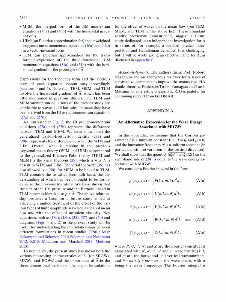
d MEM: the merged form of the EM momentum

equations (45a) and (45b) with the horizontal gradi-

ent of Ld UIM: (an Eulerian approximation for) the unweighted

isopycnal-mean momentum equations (46a) and (46b)

in a vector-invariant formd TLM: (an Eulerian approximation for the trans-

formed expression of) the three-dimensional LM

momentum equations (51a) and (51b) with the hori-

zontal gradient of the prototype of L.

Expressions for the tendency term and the Coriolis

term of each equation system vary accordingly

(sections 4 and 5). Note that TEM, MEM, and TLM

involve the horizontal gradient of L, which has been

little mentioned in previous studies. The TEM and

MEM momentum equations of the present study are

applicable to waves at all latitudes, because they have

been derived from the IB pseudomomentum equations

(27a) and (27b).

As illustrated in Fig. 2, the IB pseudomomentum

equations (27a) and (27b) represent the difference

between TEM and MEM. We have shown that the

generalized Taylor–Bretherton identity (28a) and

(28b) represents the difference between the WIM and

UIM. Overall, what is missing in the previous

isopycnal-mean theory (WIM and UIM) as compared

to the generalized Eliassen–Palm theory (TEM and

MEM) is the virial theorem (35), which is why L is

absent in WIM and UIM. The virial theorem (35) has

also allowed, via (50), for MEM to be linked to TLM.

TLM contains the so-called Bernoulli head, the un-

derstanding of which has been thought to be formi-

dable in the previous literature. We have shown that

the sum of the LM pressure and the Bernoulli head in

TLM becomes identical to p1L. The above relation-

ship provides a basis for a future study aimed at

achieving a unified treatment of the effect of the var-

ious types of finite-amplitude waves on a sheared mean

flow and with the effect of turbulent viscosity. Key

equations, such as (18a), (18b), (35), (37), and (50) and

diagrams (Figs. 1 and 2) in the present study will be

useful for understanding the interrelationships between

different formulations in recent studies (TN01; M06;

Nakamura and Solomon 2011; Solomon and Nakamura

2012; KS13; Maddison and Marshall 2013; Methven

2013).

To summarize, the present study has shown both the

various interesting characteristics of L (for MIGWs,

MRWs, and EQWs) and the importance of L in the

three-dimensional version of the major formulations

for the effect of waves on the mean flow (see TEM,

MEM, and TLM in the above list). These abundant

results, previously unmentioned, suggest a future

study dedicated to an independent investigation for Lin terms of, for example, a detailed physical inter-

pretation and Hamiltonian dynamics. It is challenging,

but it will be worth giving an effective name for L, asdiscussed in appendix C.

Acknowledgments. The authors thank Prof. Noboru

Nakamura and an anonymous reviewer for a series of

constructive comments to improve the manuscript. HA

thanks Emeritus Professors Toshio Yamagata and Taroh

Matsuno for interesting discussions. RJG is grateful for

continuing support from GEOMAR.

APPENDIX A

An Alternative Expression for the Wave EnergyAssociated with MIGWs

In this appendix, we assume that the Coriolis pa-

rameter f is a uniform constant (i.e., f 5 f0 and b5 0)

and the buoyancy frequencyN is a uniform constant (in

particular, with no variation in the vertical direction).

We shall show that the quantity (u0ty0 2 u0y0t)/(2f ) on the

right-hand side of (38) is equal to the wave energy as-

sociated with MIGWs.

We consider a Fourier integral in the form

p0(x, y, z, t)5ðP(k, l,m, u) d3k , (A1a)

u0(x, y, z, t)5ðU(k, l,m, u) d3k , (A1b)

y0(x, y, z, t)5ðV(k, l,m, u) d3k , (A1c)

w0(x, y, z, t)5ðW(k, l,m, u) d3k, and (A1d)

z0(x, y, z, t)5ðZ(k, l,m, u) d3k , (A1e)

where P, U, V, W, and Z are the Fourier constituents

associated with p0, u0, y0, w0 and z0, respectively; (k, l)and m are the horizontal and vertical wavenumbers;

and u5 kx1 ly1mz2st is the wave phase, with s

being the wave frequency. The Fourier integral is


Ðd3k[

Ð Ð Ðdk dl dm. An analytical solution for the

equation system (6a)–(6e) may be written as

P[A cosu , (A2a)

U[ (Psk1Puf l)/(s22 f 2) , (A2b)

V[ (2Pufk1Psl)/(s22 f 2) , (A2c)

W[2Psm/N2 , and (A2d)

Z[2Pum/N2 , (A2e)

where A5A(k, l, m) is wave amplitude for each

Fourier constituent, and Pu 52A sinu is understood

(Gill 1982; Holton 1992). A dispersion relation for

MIGWs is written as

k21 l2

s22 f 25

m2

N2. (A3)

Using the analytical solution (A2a)–(A2e), we calculate

the time average of the wave energy associated with

MIGWs with a general spectrum:

E5 (1/2)

ð[U2 1V21N2Z2] d3k

5 (1/2)

ð[(P2s21P2

uf2)(k2 1 l2)/(s2 2 f 2)21P2

um2/N2] d3k

5 (1/2)

ð[(P2s21P2

uf2)1P2

u(s2 2 f 2)]m2/[N2(s22 f 2)] d3k5

ðP2s2m2/[N2(s22 f 2)] d3k , (A4)

where both PPu 5 2A2 cosu sinu 5 0 and P2 5A2 cos2u5A2 sin2u5P2

u have been used, and the third

line of (A4) has been derived using the dispersion re-

lation (A3).

On the other hand, substitution of the analytical so-

lution (A2a)–(A2e) to the quantity (u0ty0 2 u0y0t)/(2f ) onthe right-hand side of (38) yields

(u0ty02 u0y0t)/(2f )

5 (1/2)

ð(P21P2

u)s2(k2 1 l2)/(s22 f 2)2 d3k

5 (1/2)

ð(P21P2

u)s2m2/[N2(s22 f 2)]d3k , (A5)

which has been written in an instantaneous expres-

sion, and the second line has been derived using

the dispersion relation (A3). Comparing the last line

of each of (A4) and (A5), one can easily see that

the time average of (A5) becomes equal to the

wave energy in (A4), with the understanding that

(1/2)(P2 1P2u)5P2 [i.e., (1/2)( cos2u1 sin2u)5 cos2u].

We conclude that (u0ty0 2 u0y0t)/(2f )5E for MIGWs

with a general spectrum. This result applies only

to MIGWs, not to MRWs or EQWs. Additional

features of the quantity (u0ty0 2 u0y0t)/f will be ex-

plained in a future study (Aiki et al. 2015, un-

published manuscript).

APPENDIX B

The Vertical Component of the VectorStreamfunction Associated with the Stokes-Drift

Velocity

For neutral waves, both j0y0 ’ 2h0u0 ’ (y0j0 2 u0h0)/2and j0u0 ’ 0 ’ h0y0 hold. Substitution of these relation-

ships to the approximated expression of the Stokes-drift

velocity in (12a) and (12b) yields

hhuStokes, yStokes,wStokesii’ 2$3 hh2z0y0, z0u0, (y0j02 u0h0)/2ii , (B1)

which includes the definition of the vertical compo-

nent of the Stokes-drift velocity wStokes. The quantity

hh2z0y0, z0u0, (y0j0 2 u0h0)/2ii is herein referred to as

the vector streamfunction associated with the Stokes-

drift velocity. Because j0 and h0 are not easily avail-

able from model output, it will be useful to rewrite

the vertical component of the streamfunction associ-

ated with the Stokes-drift velocity in terms of basic

quantities, such as u0, y0, z0, p0, q0, and N2. We shall

suggest two separate expressions. The first expression

is given by

(y0j02 u0h0)/2 ’ 2u0h05 u0q0/b , (B2)


where (11), (25c), and (25d) have been used.

Because (11) has been used, this expression is ap-

plicable to both EQWs and MRWs, but not to

MIGWs.

The second expression for the vertical component of the

vector streamfunction associated with the Stokes-drift

velocity may be obtained by applying a low-pass filter to

the virial theorem (35) and then substituting (37) to yield

(y0j02 u0h0)/25 [2K1G1L]/f 1 [(j0u01h0y0)|fflfflfflfflfflfflfflffl{zfflfflfflfflfflfflfflffl}’0

/(2f )]t

5 (2p0yp

0x1p0

xp0y)/(2f

2)|fflfflfflfflfflfflfflfflfflfflfflfflfflfflfflfflfflfflffl{zfflfflfflfflfflfflfflfflfflfflfflfflfflfflfflfflfflfflffl}’0 for plane waves

2K/f 1 (2y0p0x1 u0p0y)/(2f2)1 [(j0u01h0y0)|fflfflfflfflfflfflfflffl{zfflfflfflfflfflfflfflffl}

’0

/(2f )]t , (B3)

where the first line may be compared with the expressions

of M06 and TN01. For MIGWs, substitution of L ’ 0

(Table 2) to the first line of (B3) yields (y0j0 2 u0h0)/2 ’2K1G, which is the expression ofM06 that has originally

been derived from an analytical solution for the waves. For

MRWs, substitution of L ’ 2E (Table 2) to the first line

of (B3) yields (y0j0 2u0h0)/2 ’ 2K/f , which is consistent

with the expression of TN01 [see the third line in their

(49)] that has originally been derived from the quasi-

geostrophic equations.

The second line of (B3) may be compared with the

expression of KS13. The sum of the second and third

terms on the second line of (B3) corresponds to (2.15) of

KS13, which has originally been derived froma combined

analytical solution for MIGWs and MRWs. Kinoshita

and Sato (2014, hereafterKS14) have shown that (2.15) of

KS13 is not applicable to EQWs,B1 which we are able

to attribute to the first term on the second line of

(B3). We note that this term is nonzero for EQWs and

automatically vanishes for both MRWs and MIGWs

[see discussion after (38)]. Nevertheless, it would be

sometimes difficult in the model diagnosis to distin-

guish whether waves are nearly plane (i.e., MIGWs and

MRWs) or nonplane (i.e., EQWs) in the horizontal di-

rection, particularly at low latitudes (Brunet and Haynes

1996). Moreover, the quantity p0 [Ð tp0 dt is not easily

available from model output. Hence we shall seek an al-

ternative expression for the first term on the last line

of (B3):

(2p0yp

0x1p0

xp0y)/(2f

2)|fflfflfflfflfflfflfflfflfflfflfflfflfflfflfflfflfflfflffl{zfflfflfflfflfflfflfflfflfflfflfflfflfflfflfflfflfflfflffl}’0 for plane waves

5 (2p0yp

0tx1p0

xp0ty)/(2f

2)

’ (p0yp

0uu 2p0

up0uy)sk/(2f

2)

’ 2p0yp

0sk/f 2 ’ p0yp0x/f

2

52p0y(u02 fh0)/f 2

5 2p0y(u0/f 1 q0/b)/f|fflfflfflfflfflfflfflfflfflfflfflfflfflfflffl{zfflfflfflfflfflfflfflfflfflfflfflfflfflfflffl}

Excluded for MIGWs

,

(B4)

where the expression on the last line consists of quantities,

such as u0, p0, and q0, that are easily available from model

output. The second line of (B4) has been derived using

(25a) and (25c), the penultimate line has been derived

using (16a), and the last line has been derived using (11),

which is valid for both MRWs and EQWs (h0 52q0/b is

appropriate), but not for MIGWs (h0 52q0/b is not ap-

propriate).We suggest distinguishingwaves depending on

whether h0 6¼ 2q0/b (i.e., MIGWs) or h0 52q0/b (i.e.,

MRWs and EQWs) in the model diagnosis. For the type

of waves with h0 52q0/b, either (B2) or the combination

of (B3) and (B4) may be used.

To summarize, the two separate expressions (B2)

and (B3) are complementary to each other for the

understanding of the characteristics of the Stokes-drift

B1 KS14 did not extend (2.15) of KS13 to EQWs but presented

a separate expression for the Stokes-drift velocity associated with

zonally propagating EQWs. This is shown in (2.28) of KS14:

2u0h0 ’ (y0y0 2K1G)y/b5 (E2u0u0)y/b, a result that has been

derived from an analytical solution based on the Hermite poly-

nomials (Matsuno 1966). We suggest that a clearer way to rederive

their expression is to use the meridional component of the IB

pseudomomentum equation (27b) in the present paper and then

assume zonally propagating steady waves (u0y0 ’ 0 has already

been explained in the third-to-last paragraph of section 2h). The

assumption of vertically homogeneous waves is also necessary to

exclude the last term of (27b), which is implicit in the analytical

solution used in KS14. It is an open question what motivated them

to address their (2.28), because another expression for the

streamfunction2u0h0 ’ u0q0/b in (B2) is easily derived from fewer

assumptions and is applicable to all types of EQWs (including

meridionally propagating equatorial inertia–gravity waves) as well

as MRWs (Table 2).


velocity associated with MIGWs, MRWs, and EQWs

(Table 2). See also Constantin (2013) and references

therein for literature concerning the Stokes-drift veloc-

ity associated with EQWs.

APPENDIX C

How to Refer to the Quantity L in a Future Study

In the present study, the quantity L5 [(j0p0)x 1(h0p0)y 1 (z0p0)z]/2 has been referred to as a divergence-

form wave-induced pressure. It will be useful to find

a more appropriate name for L. The name should in-

dicate for what type of waves the quantity L becomes

nonzero. As explained below, L may become nonzero

for a type of wave that contains, in any direction, either

an ‘‘asymmetric velocity’’ structure or a ‘‘trapped

modal’’ structure.

The term ‘‘asymmetric velocity’’ is intended to de-

scribe, for example, the meridional structure of the

ageostrophic velocity associated with MRWs. The per-

turbation velocity may be decomposed as hhu0, y0, w0ii5hh2c0

y, c0x, 0ii1 hhua, ya, waii, where c0 5 p0/f0 is the

geostrophic streamfunction (see footnote 8) and

hhua, ya, waii is the ageostrophic component of velocity

associated with MRWs. Under the quasigeostrophic ap-

proximation, themomentumequations (6a) and (6b)may

be rewritten as

2c0yt 2 f0y

a2byc0x 5 0 and (C1a)

c0xt 1 f0u

a 2byc0y5 0. (C1b)

These equations indicate that, owing to the presence of

the b term, the ageostrophic velocity cannot be written

in the form of the linear combination of sine and cosine

functions in the meridional direction, even if the geo-

strophic streamfunction is written in the form of nearly

plane waves in the horizontal direction. A related dis-

cussion appears in AM78b (footnote, p. 654), which may

be traced back to Longuet-Higgins (1964). It can be said

that nonzero L for MRWs is attributed mostly to the

meridional gradient (h0p0)y, where h0 includes the effect

of the ageostrophic component of velocity ya.

The term ‘‘trappedmodal’’ is intended to describe, for

example, the meridional structure of EQWs. It can be

said that nonzero L for EQWs is attributed mostly to

(h0p0)y. On the other hand, if the buoyancy frequency N

varies in the vertical direction, waves may contain

a trapped modal structure in the vertical direction, as

has been noted for some types of oceanic internal

waves in previous studies. For simplicity, let’s consider

horizontally homogeneous waves (which may be ap-

propriate for MIGWs but not for EQWs and MRWs).

Then L ’ (z0p0)z/252(p0zp0/N2)z/2, where (9) has been

used. There is a possibility that (p0zp0/N2)z 6¼ 0 for ver-

tically trapped modal waves, although details of this will

be investigated in a future study. This remark is in

contrast to the statement ‘‘L5 0 for MIGWs and

L52E for MRWs,’’ which frequently appears in the

present paper, aimed at highlighting the difference in

the direction of the CE and IB fluxes. Careful readers

should be aware that the statement ‘‘L5 0 for MIGWs’’

is actually based on the analytical solution of vertically

plane waves, wherein N is assumed to be a vertically

uniform constant, as noted in both section 3c and

appendix A.

Taking together the asymmetric-velocity structure

and the trapped-modal structure mentioned above, Lmight be referred to as, for example, ‘‘wavecline pres-

sure’’ where ‘‘cline’’ indicates gradient in any direction

for basic wave structures. Although it is beyond the

scope of the present study, we have confirmed that Lbecomes nonzero for oceanic surface gravity waves (not

shown) and is closely related to the depth-dependent

expression of the radiation stress as formulated by Aiki

and Greatbatch (2013). Indeed, the vertical structure of

oceanic surface gravity waves is written (at the leading

order in terms of an asymptotic expansion) using an

exponential or hyperbolic function andmay be regarded

as a vertically trapped mode.

An alternative option is to refer to L as either ‘‘wave-

anisotropy pressure’’ or ‘‘guided-wave pressure,’’ ref-

erencing the directional properties of wave propagation

in a three-dimensional space.

REFERENCES

Aiki, H., and T. Yamagata, 2006: Energetics of the layer-thickness

form drag based on an integral identity.Ocean Sci., 2, 161–171,

doi:10.5194/os-2-161-2006.

——, and K. J. Richards, 2008: Energetics of the global ocean: The

role of layer-thickness form drag. J. Phys. Oceanogr., 38, 1845–

1869, doi:10.1175/2008JPO3820.1.

——, and R. J. Greatbatch, 2013: The vertical structure of the

surface wave radiation stress for circulation over a sloping

bottom as given by thickness-weighted-mean theory. J. Phys.

Oceanogr., 43, 149–164, doi:10.1175/JPO-D-12-059.1.

——, and ——, 2014: A new expression for the form stress term in

the vertically Lagrangian mean framework for the effect of

surface waves on the upper-ocean circulation. J. Phys. Oce-

anogr., 44, 3–23, doi:10.1175/JPO-D-12-0228.1.

Andrews, D. G., 1983a: A finite-amplitude Eliassen–Palm theorem

in isentropic coordinates. J. Atmos. Sci., 40, 1877–1883,

doi:10.1175/1520-0469(1983)040,1877:AFAEPT.2.0.CO;2.

——, 1983b: A conservation law for small-amplitude quasi-

geostrophic disturbances on a zonally asymmetric basic flow.

J. Atmos. Sci., 40, 85–90, doi:10.1175/1520-0469(1983)040,0085:

ACLFSA.2.0.CO;2.


http://dx.doi.org/10.5194/os-2-161-2006

http://dx.doi.org/10.1175/2008JPO3820.1

http://dx.doi.org/10.1175/JPO-D-12-059.1


http://dx.doi.org/10.1175/1520-0469(1983)040<1877:AFAEPT>2.0.CO;2

http://dx.doi.org/10.1175/1520-0469(1983)040<0085:ACLFSA>2.0.CO;2

http://dx.doi.org/10.1175/1520-0469(1983)040<0085:ACLFSA>2.0.CO;2

——, 1984: On the existence of nonzonal flows satisfying sufficient

conditions for instability.Geophys. Astrophys. Fluid Dyn., 28,

243–256, doi:10.1080/03091928408230366.

——, and M. E. McIntyre, 1976: Planetary waves in horizontal and

vertical shear: The generalized Eliassen–Palm relation and the

mean zonal acceleration. J. Atmos. Sci., 33, 2031–2048,

doi:10.1175/1520-0469(1976)033,2031:PWIHAV.2.0.CO;2.

——, and ——, 1978a: An exact theory of nonlinear waves on

a Lagrangian-mean flow. J. Fluid Mech., 89, 609–646,

doi:10.1017/S0022112078002773.

——, and ——, 1978b: On wave-action and its relatives. J. Fluid

Mech., 89, 647–664, doi:10.1017/S0022112078002785.Ardhuin, F., N. Rascle, and K. Belibassakis, 2008: Explicit

wave-averaged primitive equations using a generalized

Lagrangian mean. Ocean Modell., 20, 35–60, doi:10.1016/j.ocemod.2007.07.001.

Bleck, R., 1985: On the conversion between mean and eddy

components of potential and kinetic energy in isentropic and

isopycnic coordinates. Dyn. Atmos. Oceans, 9, 17–37,

doi:10.1016/0377-0265(85)90014-4.

Bretherton, F. P., 1966: Critical layer instability in baroclinic flows.

Quart. J. Roy. Meteor. Soc., 92, 325–334, doi:10.1002/

qj.49709239302.

——, and C. J. R. Garrett, 1968: Wavetrains in inhomogeneous

moving media. Proc. Roy. Soc. London, A302, 529–554,

doi:10.1098/rspa.1968.0034.

Brunet, G., and P. H. Haynes, 1996: Low-latitude reflection of

Rossby wave trains. J. Atmos. Sci., 53, 482–496, doi:10.1175/

1520-0469(1996)053,0482:LLRORW.2.0.CO;2.

Bühler, O., 2009: Waves and Mean Flows. Cambridge University

Press, 341 pp.

——, 2014: A gentle stroll through EP flux theory. Eur. J. Mech.,

47B, 12–15, doi:10.1016/j.euromechflu.2014.01.010.

Cai, M., and B. Huang, 2013: A dissection of energetics of the

geostrophic flow: Reconciliation of Rossby wave energy flux

and group velocity. J. Atmos. Sci., 70, 2179–2196, doi:10.1175/

JAS-D-12-0249.1.

Chang, E. K. M., and I. Orlanski, 1994: On energy flux and group ve-

locity of waves in baroclinic flows. J. Atmos. Sci., 51, 3823–3828,

doi:10.1175/1520-0469(1994)051,3823:OEFAGV.2.0.CO;2.

Charney, J., and P. Drazin, 1961: Propagation of planetary-scale

disturbances from the lower into the upper atmosphere.

J. Geophys. Res., 66, 83–109, doi:10.1029/JZ066i001p00083.

Chu, V. H., and C. C. Mei, 1970: On slowly-varying Stokes waves.

J. Fluid Mech., 41, 873–887, doi:10.1017/S0022112070000988.Constantin, A., 2013: Some three-dimensional nonlinear equatorial

flows. J. Phys.Oceanogr., 43, 165–175, doi:10.1175/JPO-D-12-062.1.

Craik, A. D. D., and S. Leibovich, 1976: A rational model for

Langmuir circulations. J. Fluid Mech., 73, 401–426,

doi:10.1017/S0022112076001420.

Dritschel, D. G., and M. E. McIntyre, 2008: Multiple jets as PV

staircases: ThePhillips effect and the resilience of eddy-transport

barriers. J. Atmos. Sci., 65, 855–873, doi:10.1175/2007JAS2227.1.

Durran, D. R., 1988: On a physical mechanism for Rossby wave

propagation. J. Atmos. Sci., 45, 4020–4022, doi:10.1175/

1520-0469(1988)045,4020:OAPMFR.2.0.CO;2.

Eckart, C., 1963: Extension of Howard’s circle theorem to adia-

batic jets. Phys. Fluids, 6, 1042–1047, doi:10.1063/1.1706860.

Eden, C., R. J. Greatbatch, and J. Willebrand, 2007: A diagnosis of

thickness fluxes in an eddy-resolving model. J. Phys. Ocean-

ogr., 37, 727–742, doi:10.1175/JPO2987.1.

Eliassen, A., and E. Palm, 1960: On the transfer of energy in sta-

tionary mountain waves. Geofys. Publ., 22, 1–23.

Gent, P. R., J. Willebrand, T. J. McDougall, and J. C. McWilliams,

1995: Parameterizing eddy-induced tracer transports in ocean

circulation models. J. Phys. Oceanogr., 25, 463–474,

doi:10.1175/1520-0485(1995)025,0463:PEITTI.2.0.CO;2.

Gill, A. E., 1982: Atmosphere–Ocean Dynamics. International

Geophysics Series, Vol. 30, Academic Press, 662 pp.

Greatbatch, R. J., 1998: Exploring the relationship between

eddy-induced transport velocity, vertical momentum trans-

fer, and the isopycnal flux of potential vorticity. J. Phys.

Oceanogr., 28, 422–432, doi:10.1175/1520-0485(1998)028,0422:

ETRBEI.2.0.CO;2.

——, 2001: A framework for mesoscale eddy parameterization

based on density-weighted averaging at fixed height. J. Phys.

Oceanogr., 31, 2797–2806, doi:10.1175/1520-0485(2001)031,2797:

AFFMEP.2.0.CO;2.

——, and T. J. McDougall, 2003: The non-Boussinesq temporal

residual mean. J. Phys. Oceanogr., 33, 1231–1239, doi:10.1175/

1520-0485(2003)033,1231:TNTRM.2.0.CO;2.

Hasselmann, K., 1971: On the mass and momentum transfer be-

tween short gravity waves and larger-scale motions. J. Fluid

Mech., 50, 189–205, doi:10.1017/S0022112071002520.

Hayashi, Y.-Y., and W. R. Young, 1987: Stable and unstable shear

modes of rotating parallel flows in shallow water. J. Fluid

Mech., 184, 477–504, doi:10.1017/S0022112087002982.

Haynes, P. H., 1988: Forced, dissipative generalizations of finite-

amplitude wave-activity conservation relations for zonal and

nonzonal basic flows. J. Atmos. Sci., 45, 2352–2362,

doi:10.1175/1520-0469(1988)045,2352:FDGOFA.2.0.CO;2.

Held, I. M., 1985: Pseudomomentum and the orthogonality of

modes in shear flows. J. Atmos. Sci., 42, 2280–2288,

doi:10.1175/1520-0469(1985)042,2280:PATOOM.2.0.CO;2.

Holliday, D., and M. E. McIntyre, 1981: On potential energy

density in an incompressible, stratified fluid. J. Fluid Mech.,

107, 221–225, doi:10.1017/S0022112081001742.Holton, J. R., 1992: An Introduction to Dynamic Meteorology. 3rd

ed. Academic Press, 511 pp.

Horinouchi, T., and S. Yoden, 1998: Wave–mean flow interaction

associated with a QBO-like oscillation simulated in a simpli-

fied GCM. J. Atmos. Sci., 55, 502–526, doi:10.1175/

1520-0469(1998)055,0502:WMFIAW.2.0.CO;2.

Hoskins, B. J., I. N. James, and G. H. White, 1983: The

shape, propagation and mean-flow interaction of large-scale

weather systems. J. Atmos. Sci., 40, 1595–1612, doi:10.1175/

1520-0469(1983)040,1595:TSPAMF.2.0.CO;2.

Ishioka, K., and S. Yoden, 1996: Numerical methods of estimating

bounds on the non-linear saturation of barotropic instability.

J. Meteor. Soc. Japan, 74, 167–174.

Iwasaki, T., 1989: A diagnostic formulation for wave-mean flow

interactions and Lagragian-mean circulation with a hybrid

vertical coordinate of pressure and isentropes. J. Meteor. Soc.

Japan, 67, 293–312.

——, 2001: Atmospheric energy cycle viewed from wave–mean-

flow interaction and Lagrangian mean circulation. J. Atmos.

Sci., 58, 3036–3052, doi:10.1175/1520-0469(2001)058,3036:

AECVFW.2.0.CO;2.

Jacobson, T., and H. Aiki, 2006: An exact energy for TRM theory.

J. Phys. Oceanogr., 36, 558–564, doi:10.1175/JPO2872.1.

Kinoshita, T., and K. Sato, 2013: A formulation of three-

dimensional residual mean flow applicable both to inertia–

gravity waves and to Rossby waves. J. Atmos. Sci., 70,1577–1602, doi:10.1175/JAS-D-12-0137.1.

——, and ——, 2014: A formulation of three-dimensional residual

mean flow and wave activity flux applicable to equatorial


http://dx.doi.org/10.1080/03091928408230366

http://dx.doi.org/10.1175/1520-0469(1976)033<2031:PWIHAV>2.0.CO;2

http://dx.doi.org/10.1017/S0022112078002773

http://dx.doi.org/10.1017/S0022112078002785

http://dx.doi.org/10.1016/j.ocemod.2007.07.001

http://dx.doi.org/10.1016/j.ocemod.2007.07.001

http://dx.doi.org/10.1016/0377-0265(85)90014-4

http://dx.doi.org/10.1002/qj.49709239302

http://dx.doi.org/10.1002/qj.49709239302

http://dx.doi.org/10.1098/rspa.1968.0034

http://dx.doi.org/10.1175/1520-0469(1996)053<0482:LLRORW>2.0.CO;2

http://dx.doi.org/10.1175/1520-0469(1996)053<0482:LLRORW>2.0.CO;2

http://dx.doi.org/10.1016/j.euromechflu.2014.01.010

http://dx.doi.org/10.1175/JAS-D-12-0249.1


http://dx.doi.org/10.1175/1520-0469(1994)051<3823:OEFAGV>2.0.CO;2

http://dx.doi.org/10.1029/JZ066i001p00083

http://dx.doi.org/10.1017/S0022112070000988


http://dx.doi.org/10.1017/S0022112076001420

http://dx.doi.org/10.1175/2007JAS2227.1

http://dx.doi.org/10.1175/1520-0469(1988)045<4020:OAPMFR>2.0.CO;2

http://dx.doi.org/10.1175/1520-0469(1988)045<4020:OAPMFR>2.0.CO;2

http://dx.doi.org/10.1063/1.1706860

http://dx.doi.org/10.1175/JPO2987.1

http://dx.doi.org/10.1175/1520-0485(1995)025<0463:PEITTI>2.0.CO;2

http://dx.doi.org/10.1175/1520-0485(1998)028<0422:ETRBEI>2.0.CO;2

http://dx.doi.org/10.1175/1520-0485(1998)028<0422:ETRBEI>2.0.CO;2

http://dx.doi.org/10.1175/1520-0485(2001)031<2797:AFFMEP>2.0.CO;2

http://dx.doi.org/10.1175/1520-0485(2001)031<2797:AFFMEP>2.0.CO;2

http://dx.doi.org/10.1175/1520-0485(2003)033<1231:TNTRM>2.0.CO;2

http://dx.doi.org/10.1175/1520-0485(2003)033<1231:TNTRM>2.0.CO;2

http://dx.doi.org/10.1017/S0022112071002520

http://dx.doi.org/10.1017/S0022112087002982

http://dx.doi.org/10.1175/1520-0469(1988)045<2352:FDGOFA>2.0.CO;2

http://dx.doi.org/10.1175/1520-0469(1985)042<2280:PATOOM>2.0.CO;2

http://dx.doi.org/10.1017/S0022112081001742

http://dx.doi.org/10.1175/1520-0469(1998)055<0502:WMFIAW>2.0.CO;2

http://dx.doi.org/10.1175/1520-0469(1998)055<0502:WMFIAW>2.0.CO;2

http://dx.doi.org/10.1175/1520-0469(1983)040<1595:TSPAMF>2.0.CO;2

http://dx.doi.org/10.1175/1520-0469(1983)040<1595:TSPAMF>2.0.CO;2

http://dx.doi.org/10.1175/1520-0469(2001)058<3036:AECVFW>2.0.CO;2

http://dx.doi.org/10.1175/1520-0469(2001)058<3036:AECVFW>2.0.CO;2

http://dx.doi.org/10.1175/JPO2872.1


waves. J. Atmos. Sci., 71, 3427–3438, doi:10.1175/

JAS-D-13-0161.1.

Lagrange, J. L., 1788: Méchanique Analitique. Chez la Veuve De-

saint, 512 pp.

Longuet-Higgins, M. S., 1953: Mass transport in water waves. Philos.

Trans.Roy. Soc.London,A245,535–581, doi:10.1098/rsta.1953.0006.

——, 1964: On group velocity and energy flux in planetary wave

motions. Deep-Sea Res. Oceanogr. Abstr., 11, 35–42,

doi:10.1016/0011-7471(64)91080-0.

——, 1969: On the transport of mass by time-varying ocean

currents. Deep-Sea Res. Abstr., 16, 431–447, doi:10.1016/

0011-7471(69)90031-X.

Maddison, J. R., and D. P. Marshall, 2013: The Eliassen–Palm flux

tensor. J. Fluid Mech., 729, 69–102, doi:10.1017/jfm.2013.259.

Masuda, A., 1978: Group velocity and energy transport by Rossby

waves. J.Oceanogr. Soc. Japan, 34, 1–7, doi:10.1007/BF02109610.

Matsuno, T., 1966: Quasi-geostrophic motions in the equatorial

area. J. Meteor. Soc. Japan, 44, 25–43.

McDougall, T. J., and P. C.McIntosh, 2001: The temporal-residual-

mean velocity. Part II: Isopycnal interpretation and the tracer

and momentum equations. J. Phys. Oceanogr., 31, 1222–1246,

doi:10.1175/1520-0485(2001)031,1222:TTRMVP.2.0.CO;2.

McPhaden, M. J., and P. Ripa, 1990: Wave–mean flow interactions

in the equatorial ocean. Annu. Rev. Fluid Mech., 22, 167–205,

doi:10.1146/annurev.fl.22.010190.001123.

Methven, J., 2013: Wave activity for large-amplitude disturbances

described by the primitive equations on the sphere. J. Atmos.

Sci., 70, 1616–1630, doi:10.1175/JAS-D-12-0228.1.

Miyahara, S., 2006: A three dimensional wave activity flux appli-

cable to inertio-gravity waves. SOLA, 2, 108–111, doi:10.2151/sola.2006-028.

Müller, P., 1995: Ertel’s potential vorticity theorem in physical

oceanography.Rev.Geophys., 33, 67–97, doi:10.1029/94RG03215.

Nakamura, N., and A. Solomon, 2011: Finite-amplitude wave ac-

tivity and mean flow adjustments in the atmospheric general

circulation. Part II: Analysis in the isentropic coordinate.

J. Atmos. Sci., 68, 2783–2799, doi:10.1175/2011JAS3685.1.

Noda,A., 2010: A general three-dimensional transformed Eulerain

mean formulation. SOLA, 6, 85–88, doi:10.2151/sola.2010-022.

Plumb, R. A., 1985: On the three-dimensional propagation of sta-

tionary waves. J. Atmos. Sci., 42, 217–229, doi:10.1175/

1520-0469(1985)042,0217:OTTDPO.2.0.CO;2.

——, 1986: Three-dimensional propagation of transient quasi-

geostrophic eddies and its relationship with the eddy forcing

of the time–mean flow. J. Atmos. Sci., 43, 1657–1678,

doi:10.1175/1520-0469(1986)043,1657:TDPOTQ.2.0.CO;2.

Rhines, P., 1982: Basic dynamics of the large-scale geostrophic

circulation. 1982 summer study program in geophysical fluid

dynamics, Woods Hole Oceanographic Institution Tech Rep.

WHOI-82-45, 1–4, doi:10.1575/1912/2895.

Ripa, P., 1982: Nonlinear wave–wave interactions in a one-layer

reduced-gravity model on the equatorial b plane. J. Phys.

Oceanogr., 12, 97–111, doi:10.1175/1520-0485(1982)012,0097:

NWIIAO.2.0.CO;2.

Sassi, F., and R. R. Garcia, 1997: The role of equatorial waves forced

by convection in the tropical semiannual oscillation. J. Atmos.

Sci., 54, 1925–1942, doi:10.1175/1520-0469(1997)054,1925:

TROEWF.2.0.CO;2.

Sato, K., and T. J. Dunkerton, 1997: Estimates of momentum flux

associated with equatorial Kelvin and gravity waves. J. Geo-

phys. Res., 102, 26 247–26 261, doi:10.1029/96JD02514.

Scinocca, J. F., and T. G. Shepherd, 1992: Nonlinear wave-activity

conservation laws and Hamiltonian structure for the two-

dimensional anelastic equations. J. Atmos. Sci., 49, 5–28,

doi:10.1175/1520-0469(1992)049,0005:NWACLA.2.0.CO;2.

Solomon, A., and N. Nakamura, 2012: An exact Lagrangian-mean

wave activity for finite-amplitude disturbances to barotropic flow

on a sphere. J. FluidMech., 693, 69–92, doi:10.1017/jfm.2011.460.

Takaya, K., and H. Nakamura, 1997: A formulation of a wave-

activity flux for stationary Rossby waves on a zonally varying

basic flow. Geophys. Res. Lett., 24, 2985–2988, doi:10.1029/

97GL03094.

——, and ——, 2001: A formulation of a phase-independent

wave-activity flux for stationary and migratory quasigeo-

strophic eddies on a zonally varying basic flow. J. Atmos.

Sci., 58, 608–627, doi:10.1175/1520-0469(2001)058,0608:

AFOAPI.2.0.CO;2.

Takehiro, S.-I., and Y.-Y. Hayashi, 1992: Over-reflection and shear

instability in a shallow-water model. J. Fluid Mech., 236, 259–

279, doi:10.1017/S0022112092001411.

Taylor, G. I., 1915: Eddy motion in the atmosphere. Philos. Trans.

Roy. Soc. London, A215, 1–23, doi:10.1098/rsta.1915.0001.

Trenberth, K. E., 1986: An assessment of the impact of transient

eddies on the zonal flow during a blocking episode using

localized Eliassen–Palm flux diagnostics. J. Atmos. Sci.,

43, 2070–2087, doi:10.1175/1520-0469(1986)043,2070:

AAOTIO.2.0.CO;2.

Tung, K. K., 1986: Nongeostrophic theory of zonally averaged

circulation. Part I: Formulation. J. Atmos. Sci., 43, 2600–2618,

doi:10.1175/1520-0469(1986)043,2600:NTOZAC.2.0.CO;2.

Uryu, M., 1974: Mean zonal flows induced by a vertically propa-

gating Rossby wave packet. J. Meteor. Soc. Japan, 52, 481–490.

Whitham, G. B., 1974: Linear and Nonlinear Waves. John Wiley &

Sons, Inc., 636 pp.

Yanai, M., and T. Maruyama, 1966: Stratospheric wave distur-

bances propagating over the equatorial Pacific. J. Meteor. Soc.

Japan, 44, 291–294.

Young, W. R., 2012: An exact thickness-weighted average formu-

lation of the Boussinesq equations. J. Phys. Oceanogr., 42,692–707, doi:10.1175/JPO-D-11-0102.1.




http://dx.doi.org/10.1098/rsta.1953.0006

http://dx.doi.org/10.1016/0011-7471(64)91080-0

http://dx.doi.org/10.1016/0011-7471(69)90031-X

http://dx.doi.org/10.1016/0011-7471(69)90031-X

http://dx.doi.org/10.1017/jfm.2013.259

http://dx.doi.org/10.1007/BF02109610

http://dx.doi.org/10.1175/1520-0485(2001)031<1222:TTRMVP>2.0.CO;2

http://dx.doi.org/10.1146/annurev.fl.22.010190.001123


http://dx.doi.org/10.2151/sola.2006-028


http://dx.doi.org/10.1029/94RG03215

http://dx.doi.org/10.1175/2011JAS3685.1


http://dx.doi.org/10.1175/1520-0469(1985)042<0217:OTTDPO>2.0.CO;2

http://dx.doi.org/10.1175/1520-0469(1985)042<0217:OTTDPO>2.0.CO;2

http://dx.doi.org/10.1175/1520-0469(1986)043<1657:TDPOTQ>2.0.CO;2

http://dx.doi.org/10.1575/1912/2895

http://dx.doi.org/10.1175/1520-0485(1982)012<0097:NWIIAO>2.0.CO;2

http://dx.doi.org/10.1175/1520-0485(1982)012<0097:NWIIAO>2.0.CO;2

http://dx.doi.org/10.1175/1520-0469(1997)054<1925:TROEWF>2.0.CO;2

http://dx.doi.org/10.1175/1520-0469(1997)054<1925:TROEWF>2.0.CO;2

http://dx.doi.org/10.1029/96JD02514

http://dx.doi.org/10.1175/1520-0469(1992)049<0005:NWACLA>2.0.CO;2

http://dx.doi.org/10.1017/jfm.2011.460

http://dx.doi.org/10.1029/97GL03094

http://dx.doi.org/10.1029/97GL03094

http://dx.doi.org/10.1175/1520-0469(2001)058<0608:AFOAPI>2.0.CO;2

http://dx.doi.org/10.1175/1520-0469(2001)058<0608:AFOAPI>2.0.CO;2

http://dx.doi.org/10.1017/S0022112092001411

http://dx.doi.org/10.1098/rsta.1915.0001

http://dx.doi.org/10.1175/1520-0469(1986)043<2070:AAOTIO>2.0.CO;2

http://dx.doi.org/10.1175/1520-0469(1986)043<2070:AAOTIO>2.0.CO;2

http://dx.doi.org/10.1175/1520-0469(1986)043<2600:NTOZAC>2.0.CO;2


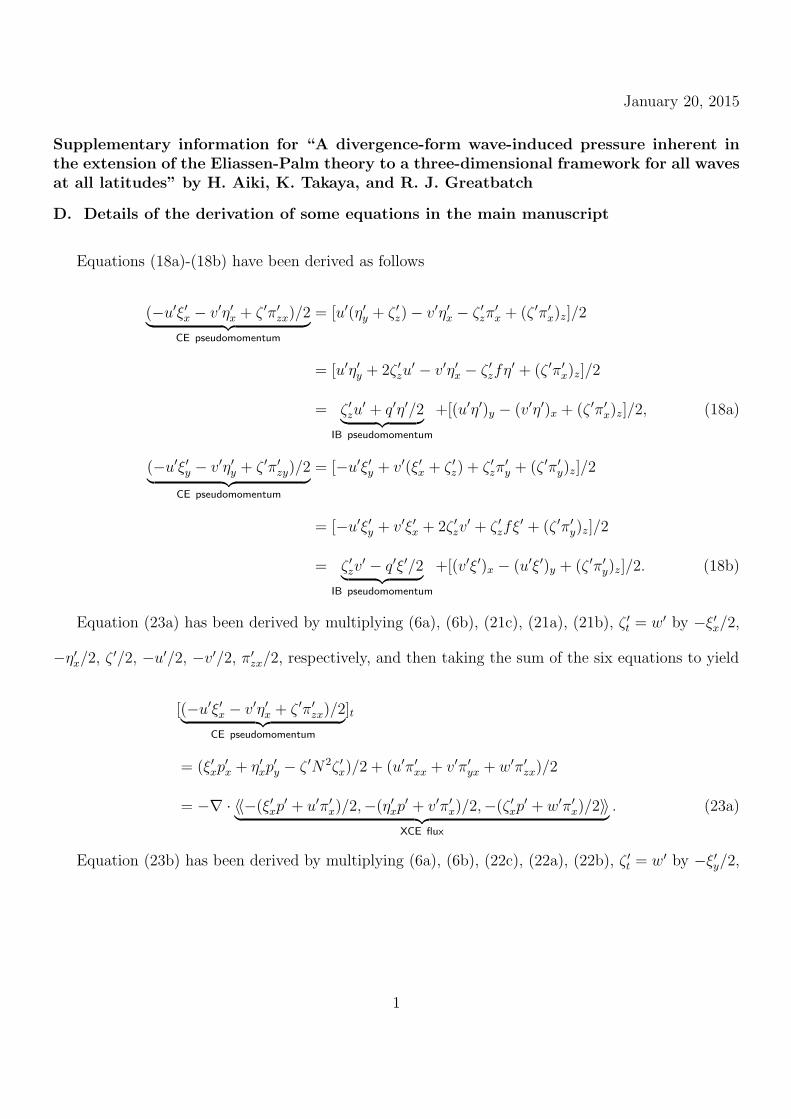
January 20, 2015

Supplementary information for “A divergence-form wave-induced pressure inherent inthe extension of the Eliassen-Palm theory to a three-dimensional framework for all wavesat all latitudes” by H. Aiki, K. Takaya, and R. J. Greatbatch

D. Details of the derivation of some equations in the main manuscript

Equations (18a)-(18b) have been derived as follows

(−u′ξ′x − v′η′x + ζ ′π′

zx)/2︸︷︷︸CE pseudomomentum

= [u′(η′y + ζ ′

z) − v′η′x − ζ ′

zπ′x + (ζ ′π′

x)z]/2

= [u′η′y + 2ζ ′

zu′ − v′η′

x − ζ ′zfη′ + (ζ ′π′

x)z]/2

= ζ ′zu

′ + q′η′/2︸︷︷︸IB pseudomomentum

+[(u′η′)y − (v′η′)x + (ζ ′π′x)z]/2, (18a)

(−u′ξ′y − v′η′y + ζ ′π′

zy)/2︸︷︷︸CE pseudomomentum

= [−u′ξ′y + v′(ξ′x + ζ ′z) + ζ ′

zπ′y + (ζ ′π′

y)z]/2

= [−u′ξ′y + v′ξ′x + 2ζ ′zv

′ + ζ ′zfξ′ + (ζ ′π′

y)z]/2

= ζ ′zv

′ − q′ξ′/2︸︷︷︸IB pseudomomentum

+[(v′ξ′)x − (u′ξ′)y + (ζ ′π′y)z]/2. (18b)

Equation (23a) has been derived by multiplying (6a), (6b), (21c), (21a), (21b), ζ ′t = w′ by −ξ′x/2,

−η′x/2, ζ ′/2, −u′/2, −v′/2, π′

zx/2, respectively, and then taking the sum of the six equations to yield

[(−u′ξ′x − v′η′x + ζ ′π′

zx)/2︸︷︷︸CE pseudomomentum

]t

= (ξ′xp′x + η′

xp′y − ζ ′N2ζ ′

x)/2 + (u′π′xx + v′π′

yx + w′π′zx)/2

= −∇ · ⟨⟨−(ξ′xp′ + u′π′

x)/2,−(η′xp

′ + v′π′x)/2,−(ζ ′

xp′ + w′π′

x)/2⟩⟩︸︷︷︸XCE flux

. (23a)

Equation (23b) has been derived by multiplying (6a), (6b), (22c), (22a), (22b), ζ ′t = w′ by −ξ′y/2,

1

−η′y/2, ζ ′/2, −u′/2, −v′/2, π′

zy/2, respectively, and then taking the sum of the six equations to yield,

[(−u′ξ′y − v′η′y + ζ ′π′

zy)/2︸︷︷︸CE pseudomomentum

]t

= (ξ′yp′x + η′

yp′y − ζ ′N2ζ ′

y)/2 + (u′π′xy + v′π′

yy + w′π′zy)/2 + β(v′ξ′ − u′η′)/2

= −∇ · ⟨⟨−(ξ′yp′ + u′π′

y)/2,−(η′yp

′ + v′π′y)/2,−(ζ ′

yp′ + w′π′

y)/2⟩⟩︸︷︷︸YCE flux

+β(v′ξ′ − u′η′)/2. (23b)

Equations (27a) has been derived as follows.

( ζ ′zu

′ + q′η′/2︸︷︷︸IB pseudomomentum

)t = ζ ′ztu

′ + ζ ′z(−p′x + fv′) + q′t︸︷︷︸

−βv′

η′/2 + q′︸︷︷︸−βη′

v′/2

= w′zu

′ − ζ ′zp

′x + (fζ ′

z − βη′︸︷︷︸v′

x−u′y

)v′

= −(u′x + v′

y)u′ − ζ ′

zp′x + (v′

x − u′y)v

′

= −(u′u′)x − (v′u′)y + Kx − ζ ′zp

′x

= −(u′u′)x − (v′u′)y + Kx + ζ ′p′xz − (ζ ′p′x)z

= −∇ · ⟨⟨u′u′−K+G︷︸︸︷E − v′v′, v′u′, ζ ′p′x⟩⟩︸︷︷︸

XIB flux

, (27a)

where K ≡ (u′2 + v′2)/2 is the wave kinetic energy and G ≡ (N2/2)ζ ′2 is the wave potential energy.

The second line of (27a) has been derived using (10)-(11), and the last line has been derived using

both (9) and E = K + G.

2

Equation (27b) has been derived as follows,

( ζ ′zv

′ − q′ξ′/2︸︷︷︸IB pseudomomentum

)t = ζ ′ztv

′ + ζ ′z(−p′y − fu′) − q′t︸︷︷︸

−βv′

ξ′/2 − q′︸︷︷︸−βη′

u′/2

= w′zv

′ − ζ ′zp

′y − (fζ ′

z − βη′︸︷︷︸v′

x−u′y

)u′ + β(v′ξ′ − u′η′)/2

= −(u′x + v′

y)v′ − ζ ′

zp′y − (v′

x − u′y)u

′ + β(v′ξ′ − u′η′)/2

= −(u′v′)x − (v′v′)y + Ky − ζ ′zp

′y + β(v′ξ′ − u′η′)/2

= −(u′v′)x − (v′v′)y + Ky + ζ ′p′yz − (ζ ′p′y)z + β(v′ξ′ − u′η′)/2

= −∇ · ⟨⟨v′u′,

v′v′−K+G︷︸︸︷E − u′u′, ζ ′p′y⟩⟩︸︷︷︸

YIB flux

+β(v′ξ′ − u′η′)/2, (27b)

where the second line has been derived using (10)-(11), and the last line has been derived using both

(9) and E = K + G.

Equations (33a)-(33f) have been derived as follows.

(ξ′p′x − u′π′x)/2 − Λ = [u′(u′ − fη′) − ξ′(u′

t − fv′)]/2 − Λ

= E − (v′v′ − η′v′t)/2

= E − v′v′ + (v′η′)t/2, (33a)

(η′p′x − v′π′x)/2 = [v′(fη′ − π′

x) − η′(fv′ − p′x)]/2

= (v′u′ − η′u′t)/2

= v′u′ − (u′η′)t/2, (33b)

(ζ ′p′x − w′π′x)/2 = ζ ′p′x − (ζ ′π′

x)t/2, (33c)

3

(ξ′p′y − u′π′y)/2 = [u′(−fξ′ − π′

y) − ξ′(−fu′ − p′y)]/2

= (u′v′ − ξ′v′t)/2

= u′v′ − (v′ξ′)t/2, (33d)

(η′p′y − v′π′y)/2 − Λ = [v′(v′ + fξ′) − η′(v′

t + fu′)]/2 − Λ

= E − (u′u′ − ξ′u′t)/2

= E − u′u′ + (u′ξ′)t/2, (33e)

(ζ ′p′y − w′π′y)/2 = ζ ′p′y − (ζ ′π′

y)t/2, (33f)

where the first line of each of (33a) and (33e) has been derived using the set of (6a)-(6b) and (16a)-

(16b), and the second line of each of (33a) and (33e) has been derived using (32).

Equations (49a)-(49b) have been derived as follows,

ζ ′u′z − η′q′/2︸︷︷︸

DI wave activity

= ζ ′u′z + η′q′/2 − η′q′

= ζ ′u′z − βη′2/2 − η′(v′

x − u′y − fζ ′

z)

= −(ξ′u′ + η′v′)x − (fξ′η′)x/2 − (fη′2)y/2

+ (ξ′u′x + η′u′

y + ζ ′u′z)︸︷︷︸

uStokes

− [−u′ξ′x − v′η′x + f(ξ′xη

′ − ξ′η′x)/2]︸︷︷︸

GL pseudomomentum

, (49a)

ζ ′v′z + ξ′q′/2︸︷︷︸

DI wave activity

= ζ ′v′z − ξ′q′/2 + ξ′q′

= ζ ′v′z + βξ′η′/2 + ξ′(v′

x − u′y − fζ ′

z)

= −(ξ′u′ + η′v′)y + (fξ′2)x/2 + (fξ′η′)y/2

+ (ξ′v′x + η′v′

y + ζ ′v′z)︸︷︷︸

vStokes

− [−u′ξ′y − v′η′y + f(ξ′yη

′ − ξ′η′y)/2]︸︷︷︸

GL pseudomomentum

, (49b)

where the second line of each equation has been derived using both (11) and q′ ≡ v′x − u′

y − fζ ′z, and

uStokes and vStokes on the last line have been defined in (12a)-(12b).

4

E. Nonhydrostatic IB pseudomomentum and wave-activity

This section investigates the first part of the DI wave-activity in (20a)-(20b). Below we show that

⟨⟨ζ ′u′z, ζ

′v′z⟩⟩ represents a hydrostatic approximation for ⟨⟨ζ ′(u′

z − w′x), ζ

′(v′z − w′

y)⟩⟩ that has been used

in the nonhydrostatic gravity wave literature, in the limit of no vertical shear of mean flows. See Eq.

(6.16) of SS92 for the expression in the presence of the vertical shear of mean flows.

An equation system for nonhydrostatic linear waves in a rotating stratified fluid may be written

as,

u′t − fv′ = −(p′ + pn)x, (E1a)

v′t + fu′ = −(p′ + pn)y, (E1b)

w′t = −pn

z , (E1c)

where p′ is hydrostatic pressure, which is defined by (6d), and pn is nonhydrostatic pressure. The

Coriolis parameter is f = f0 + βy. Using (8) and nonhydrostatic versions of (16a)-(16b), we expand

the zonal and meridional components of the nonhydrostatic version of the CE pseudomomentum in

(17) to read,

(−u′ξ′x − v′η′x − w′ζ ′

x + ζ ′π′zx)/2︸︷︷︸

nonhydrostatic CE pseudomomentum

= [u′(η′y + ζ ′

z) − v′η′x − w′ζ ′

x − ζ ′zπ

′x + (ζ ′π′

x)z]/2

= [u′η′y + 2ζ ′

zu′ − v′η′

x − w′ζ ′x + ζ ′

z(−fη′ + πnx) + (ζ ′π′

x)z]/2

= ζ ′zu

′ + ζ ′w′x + q′η′/2︸︷︷︸

nonhydrostatic IB pseudomomentum

+[(u′η′)y − (v′η′ + w′ζ ′)x + (ζ ′π′x + ζ ′πn

x)z]/2, (E2a)

5

(−u′ξ′y − v′η′y − w′ζ ′

y + ζ ′π′zy)/2︸︷︷︸

nonhydrostatic CE pseudomomentum

= [−u′ξ′y + v′(ξ′x + ζ ′z) − w′ζ ′

y − ζ ′zπ

′y + (ζ ′π′

y)z]/2

= [−u′ξ′y + v′ξ′x + 2ζ ′zv

′ − w′ζ ′y + ζ ′

z(fξ′ + πny ) + (ζ ′π′

y)z]/2

= ζ ′zv

′ + ζ ′w′y − q′ξ′/2︸︷︷︸


+[(v′ξ′)x − (u′ξ′ + w′ζ ′)y + (ζ ′π′y + ζ ′πn

y )z]/2, (E2b)

where (8) and the nonhydrostatic version of (16a)-(16b) have been used with πn ≡∫ t

pndt. Equations

(E2a)-(E2b) correspond to (18a)-(18b). As in (20a)-(20b), we suggest to refer the difference of the

quasi-Stokes velocity and the nonhydrostatic IB pseudomomentum as the nonhydrostatic DI wave-

activity,

(ζ ′u′)z︸︷︷︸uqs

− (ζ ′zu

′ + ζ ′w′x + η′q′/2)︸︷︷︸


= ζ ′(u′z − w′

x) − η′q′/2︸︷︷︸nonhydrostatic DI wave−activity

, (E3a)

(ζ ′v′)z︸︷︷︸vqs

− (ζ ′zv

′ + ζ ′w′y − ξ′q′/2)︸︷︷︸


= ζ ′(v′z − w′

y) + ξ′q′/2︸︷︷︸nonhydrostatic DI wave−activity

, (E3b)

where the first term on the right hand side is indeed the same as the wave-activity used in the gravity

wave literature except that the vertical shear of mean flows is assumed to be absent in the present

study. We conclude that ⟨⟨ζ ′u′z, ζ

′v′z⟩⟩, which is the first part of the DI wave-activity in (20a)-(20b),

represents a hydrostatic approximation for ⟨⟨ζ ′(u′z − w′

x), ζ′(v′

z − w′y)⟩⟩.

For readers who might be interested, we show prognostic equations for the nonhydrostatic IB

pseudomomentum to read,

[ ζ ′zu

′ + ζ ′w′x + q′η′/2︸︷︷︸


]t

= −[u′u′ − (u′2 + v′2 + w′2 − N2ζ ′2)/2]x − [v′u′]y − [ζ ′(p′ + pn)x]z, (E4a)

[ ζ ′zv

′ + ζ ′w′y − q′ξ′/2︸︷︷︸


]t

= −[v′u′]x − [v′v′ − (u′2 + v′2 + w′2 − N2ζ ′2)/2]y − [ζ ′(p′ + pn)y]z + β(v′ξ′ − u′η′)/2. (E4b)

Equations (E4a)-(E4b) have been derived using (10)-(11) and (E1a)-(E1c). We have omitted the

6

details of the derivation of (E4b)-(E4b), because it is essentially the same as that in the hydrostatic

IB pseudomomentum equations (27a)-(27b).

7

a divergence-form wave-induced pressure inherent in the … · 2015-07-09 · a divergence-form...

Documents