a discrete theory of connections on principal bundles

A DISCRETE THEORY OF CONNECTIONS ON PRINCIPAL BUNDLES

MELVIN LEOK, JERROLD E. MARSDEN, AND ALAN D. WEINSTEIN

Abstract. Connections on principal bundles play a fundamental role in expressing the equations of motion

for mechanical systems with symmetry in an intrinsic fashion. A discrete theory of connections on principal

bundles is constructed by introducing the discrete analogue of the Atiyah sequence, with a connectioncorresponding to the choice of a splitting of the short exact sequence. Equivalent representations of a discrete

connection are considered, and an extension of the pair groupoid composition, that takes into account the

principal bundle structure, is introduced. Computational issues, such as the order of approximation, arealso addressed. Discrete connections provide an intrinsic method for introducing coordinates on the reduced

space for discrete mechanics, and provide the necessary discrete geometry to introduce more general discrete

symmetry reduction. In addition, discrete analogues of the Levi-Civita connection, and its curvature, areintroduced by using the machinery of discrete exterior calculus, and discrete connections.

Contents

1. Introduction 12. General Theory of Bundles 63. Connections and Bundles 74. Discrete Connections 105. Geometric Structures Derived from the Discrete Connection 246. Computational Aspects 287. Applications 328. Conclusions and Future Work 37References 37

1. Introduction

One of the major goals of geometric mechanics is the study of symmetry, and its consequences. Animportant tool in this regard is the non-singular reduction of mechanical systems under the action of freeand proper symmetries, which is naturally formulated in the setting of principal bundles.

The reduction procedure results in the decomposition of the equations of motion into terms involving theshape and group variables, and the coupling between these are represented in terms of a connection on theprincipal bundle.

Connections and their associated curvature play an important role in the phenomena of geometric phases.A discussion of the history of geometric phases can be found in Berry [1990]. Shapere and Wilczek [1989]is a collection of papers on the theory and application of geometric phases to physics. In the rest of thissection, we will survey some of the applications of geometric phases and connections to geometric mechanicsand control, some of which were drawn from Marsden [1994, 1997], Marsden and Ratiu [1999].

1

2 MELVIN LEOK, JERROLD E. MARSDEN, AND ALAN D. WEINSTEIN

The simulation of these phenomena requires the construction of a discrete notion of connections onprincipal bundles that is compatible with the approach of discrete variational mechanics, and it towards thisend that this chapter is dedicated.

Falling Cat. Geometric phases arise in nature, and perhaps the most striking example of this is the fallingcat, which is able to reorient itself by 180◦, while remaining at zero angular momentum, as show in Figure 1.

The key to reconciling this with the constancy of the angular momentum is that angular momentumdepends on the moment of inertia, which in turn depends on the shape of the cat. When the cat changes itshape by curling up and twisting, its moment of inertia changes, which is in turn compensated by its overallorientation changing to maintain the zero angular momentum condition. The zero angular momentumcondition induces a connection on the principal bundle, and the curvature of this connection is what allowsthe cat to reorient itself.

A similar experiment can be tried on Earth, as described on page 10 of Vedral [2003]. This involvesstanding on a swivel chair, lifting your arms, and rotating them over your head, which will result in the chairswivelling around slowly.

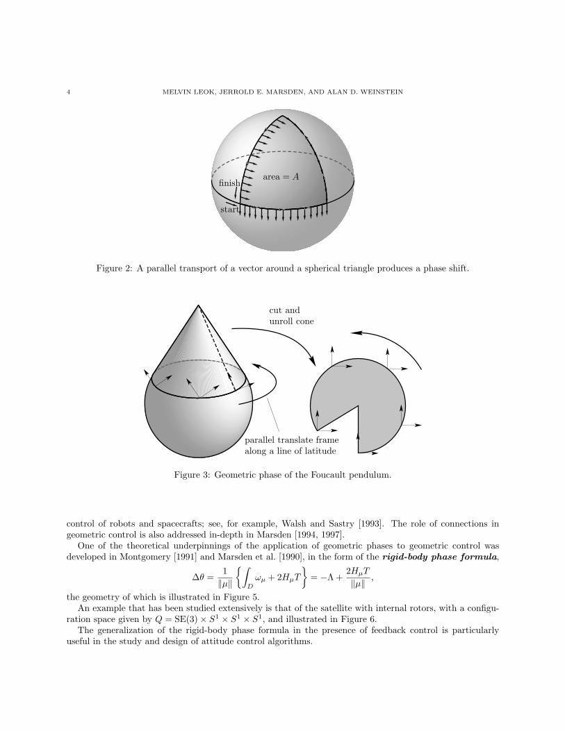
Holonomy. The sense in which curvature is related to geometric phases is most clearly illustrated byconsidering the parallel transport of a vector around a curve on the sphere, as shown in Figure 2.

Think of the point on the sphere as representing the shape of the cat, and the vector as representing itsorientation. The fact that the vector experiences a phase shift when parallel transported around the sphereis an example of holonomy. In general, holonomy refers to a situation in geometry wherein an orthonormalframe that is parallel transported around a closed loop, back to its original position, is rotated with respectto its original orientation.

Curvature of a space is critically related to the presence of holonomy. Indeed, curvature should be thoughtof as being an infinitesimal version of holonomy, and this interpretation will resurface when considering thediscrete analogue of curvature in the context of a discrete exterior calculus.

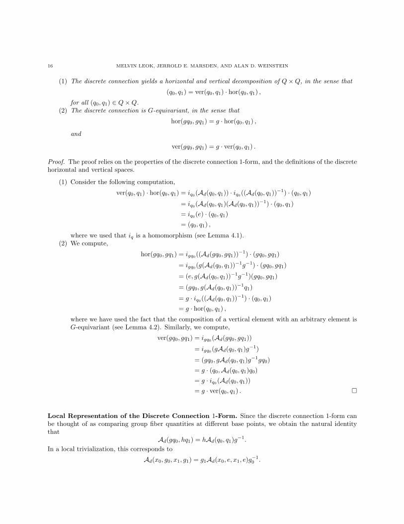
Foucault Pendulum. Another example relating geometric phases and holonomy is that of the Foucaultpendulum. As the Earth rotates about the Sun, the Foucault pendulum exhibits a phase shift of ∆θ =2π cos α (where α is the co-latitude). This phase shift is geometric in nature, and is a consequence ofholonomy. If one parallel transports an orthonormal frame around the line of constant latitude, it exhibitsa phase shift that is identical to that of the Foucault pendulum, as illustrated in Figure 3.

True Polar Wander. A particular striking example of the consequences of geometric phases and theconservation of angular momentum is the phenomena of true polar wander, that was studied by Goldreichand Toomre [1969], and more recently by Leok [1998]. It is thought that some 500 to 600 million years ago,during the Vendian–Cambrian transition, the Earth, over a 15-million-year period, experienced an inertialinterchange true polar wander event. This occurred when the intermediate and maximum moments of inertiacrossed due to the redistribution of mass anomalies, associated with continental drift and mantle convection,thereby causing a catastrophic shift in the axis of rotation.

This phenomena is illustrated in Figure 4, wherein the places corresponding to the North and South polesof the Earth migrate towards the equator as the axis of rotation changes.

Geometric Control Theory. Geometric phases also have interesting applications and consequences ingeometric control theory, and allow, for example, astronauts in free space to reorient themselves by changingtheir shape. By holding one of their legs straight, swivelling at the hip, and moving their foot in a circle,they are able to change their orientation. Since the reorientation only occurs as the shape is being changed,this allows the reorientation to be done with extremely high precision. Such ideas have been applied to the

A DISCRETE THEORY OF CONNECTIONS ON PRINCIPAL BUNDLES 3

c© Gerard Lacz/Animals Animals

Figure 1: Reorientation of a falling cat at zero angular momentum.


start

finisharea = A

Figure 2: A parallel transport of a vector around a spherical triangle produces a phase shift.

parallel translate framealong a line of latitude

cut andunroll cone

Figure 3: Geometric phase of the Foucault pendulum.

control of robots and spacecrafts; see, for example, Walsh and Sastry [1993]. The role of connections ingeometric control is also addressed in-depth in Marsden [1994, 1997].

One of the theoretical underpinnings of the application of geometric phases to geometric control wasdeveloped in Montgomery [1991] and Marsden et al. [1990], in the form of the rigid-body phase formula,

∆θ =1‖µ‖

{∫D

ωµ + 2HµT

}= −Λ +

2HµT

‖µ‖,

the geometry of which is illustrated in Figure 5.An example that has been studied extensively is that of the satellite with internal rotors, with a configu-

ration space given by Q = SE(3)× S1 × S1 × S1, and illustrated in Figure 6.The generalization of the rigid-body phase formula in the presence of feedback control is particularly

useful in the study and design of attitude control algorithms.


Figure 4: True Polar Wander. Red axis corresponds to the original rotational axis, and the gold axiscorresponds to the instantaneous rotational axis.

Pµ

geometric phase

dynamic phase

true trajectory

horizontal lift

reduced trajectory

πµ

Pµ

D

Figure 5: Geometry of rigid-body phase.


spinning rotors

rigid carrier

Figure 6: Rigid body with internal rotors.

2. General Theory of Bundles

Before considering the discrete analogue of connections on principal bundles, we will review some basicmaterial on the general theory of bundles, fiber bundles, and principal fiber bundles. A more in-depthdiscussion of fiber bundles can be found in Steenrod [1951] and Kobayashi and Nomizu [1963].

A bundle Q consists of a triple (Q,S, π), where Q and S are topological spaces, respectively referred to asthe bundle space and the base space, and π : Q → S is a continuous map called the projection. We mayassume, without loss of generality, that π is surjective, by considering the bundle over the image π(Q) ⊂ S.

The fiber over the point x ∈ S, denoted Fx, is given by, Fx = π−1(x). In most situations of practicalinterest, the fiber at every point is homeomorphic to a common space F , in which case, F is the fiber of thebundle, and the bundle is a fiber bundle. The geometry of a fiber bundle is illustrated in Figure 7.

Fx Q

π

Sx

Figure 7: Geometry of a fiber bundle.

A bundle (Q,S, π) is a G-bundle if G acts on Q by left translation, and it is isomorphic to (Q,Q/G, πQ/G),where Q/G is the orbit space of the G action on Q, and πQ/G is the natural projection.

If G acts freely on Q, then (Q,S, π) is called a principal G-bundle, or principal bundle, and G is itsstructure group. G acting freely on Q implies that each orbit is homeomorphic to G, and therefore, Q isa fiber bundle with fiber G.

To make the setting for the rest of this chapter more precise, we will adopt the following definition of aprincipal bundle,


Definition 2.1. A principal bundle is a manifold Q with a free left action, ρ : G×Q → Q, of a Lie groupG, such that the natural projection, π : Q → Q/G, is a submersion. The base space Q/G is often referred toas the shape space S, which is a terminology originating from reduction theory.

We will now consider a few standard techniques for combining bundles together to form new bundles.These methods include the fiber product, Whitney sum, and the associated bundle construction.

Fiber Product. Given two bundles with the same base space, we can construct a new bundle, referred toas the fiber product, which has the same base space, and a fiber which is the direct product of the fibersof the original two bundles. More formally, we have,

Definition 2.2. Given two bundles πi : Qi → S, i = 1, 2, the fiber product is the bundle,

π1 ×S π2 : Q1 ×S Q2 → S,

where Q1 ×S Q2 is the set of all elements (q1, q2) ∈ Q1 × Q2 such that π1(q1) = π2(q2), and the projectionπ1 ×S π2 is naturally defined by π1 ×S π2(q1, q2) = π1(q1) = π2(q2). The fiber is given by (π1 ×Q π2)−1(x) =π−1

1 (x)× π−12 (x).

Whitney Sum. The Whitney sum combines two vector bundles using the fiber product construction.

Definition 2.3. Given two vector bundles τi : Vi → Q, i = 1, 2, with the same base, their Whitney sumis their fiber product, and it is a vector bundle over Q, and is denoted V1 ⊕ V2. This bundle is obtained bytaking the fiberwise direct sum of the fibers of V1 and V2.

Associated Bundle. Given a principal bundle, π : Q → Q/G, and a left action, ρ : G ×M → M , of theLie group G on a manifold M , we can construct the associated bundle.

Definition 2.4. An associated bundle M with standard fiber M is,

M = Q×G M = (Q×M)/G,

where the action of G on Q × M is given by g(q, m) = (gq, gm). The class (or orbit) of (q, m) is denoted[q, m]G or simply [q, m]. The projection πM : Q×G M → Q/G is given by,

πM : ([q, m]G) = π(q) ,

and it is easy to check that it is well-defined and is a surjective submersion.

3. Connections and Bundles

Before formally introducing the precise definition of a connection, we will attempt to develop some intuitionand motivation for the concept. As alluded to in the introduction to this chapter, a connection describes thecurvature of a space. In the classical Riemannian setting used by Einstein in his theory of general relativity,the curvature of the space is constructed out of the connection, in terms of the Christoffel symbols thatencode the connection in coordinates.

In the context of principal bundles, the connection provides a means of decomposing the tangent spaceto the bundle into complementary spaces, as show in Figure 8. Directions in the bundle that project tozero on the base space are called vertical directions, and a connection specifies a set of directions, calledhorizontal directions, at each point, which complements the space of vertical directions.


vertical directionhorizontal direction

geometric phase

bundle projection

bundle

base space

Figure 8: Geometric phase and connections.

In the rest of this section, we will formally define connections on principal bundles, and in the next section,discrete connections will be introduced in a parallel fashion.

Short Exact Sequence. This decomposition of the tangent space TQ into horizontal and vertical subspacesyields the following short exact sequence of vector bundles over Q,

0 // V Q // TQπ∗ // π∗TS // 0 ,

where V Q is the vertical subspace of TQ, and π∗TS is the pull-back of TS by the projection π : Q → S.

Atiyah Sequence. When the short exact sequence above is quotiented modulo G, we obtain an exactsequence of vector bundles over S,

0 // gi // TQ/G

π∗ // TS // 0 ,

which is called the Atiyah sequence (see, for example Atiyah [1957], Almeida and Molino [1985], Mackenzie[1995]). Here, g is the adjoint bundle, which is a special case of an associated bundle (see Definition 2.4).In particular,

g = Q×G g = (Q× g)/G ,

where the action of G on Q×g is given by g(q, ξ) = (gq,Adgξ), and πg : g → S is given by πg([q, ξ]G) = π(q).The maps in the Atiyah sequence, i : (Q× g)/G → TQ/G and π∗ : TQ/G → TS, are given by

i([q, ξ]G) = [ξQ(q)]G,

andπ∗([vq]G) = Tπ(vq).

Connection 1-form. Given a connection on a principal fiber bundle π : Q → Q/G, we can represent this asa Lie algebra-valued connection 1-form, A : TQ → g, constructed as follows (see, for example, Kobayashiand Nomizu [1963]). Given an element of the Lie algebra ξ ∈ g, the infinitesimal generator map ξ 7→ ξQ

yields a linear isomorphism between g and VqQ for each q ∈ Q. For each vq ∈ TqQ, we define A(vq) to bethe unique ξ ∈ g such that ξQ is equal to the vertical component of vq.

Proposition 3.1. The connection 1-form, A : TQ → g, of a connection satisfies the following conditions.


(1) The 1-form is G-equivariant, that is,

A ◦ TLg = Adg ◦A ,

for every g ∈ G, where Ad denotes the adjoint representation of G in g.(2) The 1-form induces a splitting of the Atiyah sequence, that is,

A(ξQ) = ξ ,

for every ξ ∈ g.Conversely, given a g-valued 1-form A on Q satisfying conditions 1 and 2, there is a unique connection inQ whose connection 1-form is A.

Proof. See page 64 of Kobayashi and Nomizu [1963]. �

Horizontal Lift. The horizontal lift of a vector field X ∈ X(S) is the unique vector field Xh ∈ X(Q)which is horizontal and which projects onto X, that is, Tπq(Xh

q ) = Xπ(q) for all q ∈ Q. The horizontal liftis in one-to-one correspondence with the choice of a connection on Q, as the following proposition states.

Proposition 3.2. Given a connection in Q, and a vector field X ∈ X(S), there is a unique horizontal liftXh of X. The lift Xh is left-invariant under the action of G. Conversely, every horizontal vector field Xh

on Q that is left-invariant by G is the lift of a vector field X ∈ X(S).

Proof. See page 65 of Kobayashi and Nomizu [1963]. �

Connection as a Splitting of the Atiyah Sequence. Consider the continuous Atiyah sequence,

0 // gi //

oo(π1,A)

___ TQ/Gπ∗ //

oo

Xh

___ TS // 0

We see that the connection 1-form, A : TQ → g, induces a splitting of the continuous Atiyah sequence, since

(π1,A) ◦ i([q, ξ]G) = (π1,A)([ξQ(q)]g) = [q,A(ξQ(q))]G = [q, ξ]G, for all q ∈ Q, ξ ∈ g,

which is to say that (π1,A) ◦ i = 1g. Conversely, given a splitting of the continuous Atiyah sequence, we canextend the map, by equivariance, to yield a connection 1-form.

The horizontal lift also induces a splitting on the continuous Atiyah sequence, since, by definition, thehorizontal lift of a vector field X ∈ X(S) projects onto X, which is to say that π∗ ◦Xh = 1TS . The horizontallift and the connection are related by the fact that

1TQ/G = i ◦ (π1,A) + Xh ◦ π∗,

which is a simple consequence of the fact that the two splittings are part of the following commutativediagram,

0 // g

1g

i //oo(π1,A)

___ TQ/Gπ∗ //

oo

Xh

___

αA

��

TS

1T S

// 0

0 // gi1 //

ooπ1

___ g⊕ TSπ2 //

ooi2

___ TS // 0

where αA is an isomorphism. The isomorphism is given in the following lemma.

Lemma 3.3. The map αA : TQ/G → g⊕ TS defined by

αA([q, q]G) = [q,A(q, q)]G ⊕ Tπ(q, q),

is a well-defined vector bundle isomorphism. The inverse of αA is given by

α−1A ([q, ξ]G ⊕ (x, x)) = [(x, x)h

q + ξq]G.


Proof. See page 15 of Cendra et al. [2001]. �

This lemma, and its higher-order generalization, that identifies T (2)Q/G with T (2)S ×S 2g, is critical inallowing us to construct the Lagrange–Poincare operator, which is an intrinsic method of expressing thereduced equations arising from Lagrangian reduction.

In the next section, we will develop the theory of discrete connections on principal bundles in a parallelfashion to the way we introduced continuous connections.

4. Discrete Connections

Discrete variational mechanics is based on the idea of approximating the tangent bundle TQ of Lagrangianmechanics with the pair groupoid Q×Q. As such, the purpose of a discrete connection is to decompose thesubset of Q×Q that projects to a neighborhood of the diagonal of S×S into horizontal and vertical spaces.

The reason why we emphasize that the construction is only valid for the subset of Q × Q that projectsto a neighborhood of the diagonal of S × S is that there are topological obstructions to globalizing theconstruction to all of Q×Q except in the case that Q is a trivial bundle.

One of the challenges of dealing with the discrete space modelled by the pair groupoid Q × Q is that itis not a linear space, in contrast to TQ. As we shall see, the standard pair groupoid composition is notsufficient to make sense of the notion of an element (q0, q1) ∈ Q ×Q being the composition of a horizontaland a vertical element. We will propose a natural notion of composing an element with a vertical elementthat makes sense of the horizontal and vertical decomposition.

In the subsequent sections, we will use the discrete connection to extend the pair groupoid compositioneven further, and explore its applications to the notion of curvature in discrete geometry.

Intrinsic Representation of the Tangent Bundle. The intuition underlying our construction of discretehorizontal and vertical spaces is best developed by considering the intrinsic representation of the tangentbundle. This representation is obtained by identifying a tangent vector at a point on the manifold with theequivalence class of curves on the manifold going through the point, such that the tangent to the curve atthe point is given by the tangent vector. This notion is illustrated in Figure 9.

Figure 9: Intrinsic representation of the tangent bundle.

Given a vector vq ∈ TQ, we identify it with the family of curves q : R → Q, such that q(0) = q, andq(0) = v. The equivalence class [ · ] identifies curves with the same basepoint, and the same velocity at thebasepoint.

With this representation, it is natural to consider (q0, q1) ∈ Q×Q to be an approximation of [q(·)] = vq ∈TQ, in the sense that,

q0 = q(0), q1 = q(h),


for some fixed time step h, and where q(·) is a representative curve corresponding to vq in the intrinsicrepresentation of the tangent bundle.

4.1. Horizontal and Vertical Subspaces of Q×Q. Recall that the vertical subspace at a point q, denotedVq, is given by

Vq = {vq ∈ TQ | π∗(vq) = 0} = {ξQ | ξ ∈ g}.Notice that the vertical space is precisely that subspace of TQ which maps under the lifted projection mapto the embedded copy of S in TS. We proceed in an analogous fashion to define a discrete vertical subspaceat a point q.

The natural discrete analogue of the lifted projection map π∗ is the diagonal action of the projection mapon Q×Q, (π, π) : Q×Q → Q×Q, where (q0, q1) 7→ (πq0, πq1). This is because

π∗(vq) = π∗([q(·)]) = [π(q(·))].In the same way that we embed S into TS by the map x 7→ [x] = 0x, S naturally embeds itself into thediagonal of S × S, x 7→ (x, x) = eS×S , which we recall is the identity subspace of the pair groupoid.

The alternative description of the vertical space is in terms of the embedding of Q × g into TQ, by(q, ξ) 7→ ξQ(q), using the infinitesimal generator construction,

ξQ(q) = [exp(ξt)q].

In an analogous fashion, we construct a discrete generator map, which is given in the following definition.

Definition 4.1. The discrete generator is the map i : Q×G → Q×Q, given by

i(q, g) = (q, gq),

which we also denote by iq(g) = i(q, g) = (q, gq).

Then, we have the following definition of the discrete vertical space.

Definition 4.2. The discrete vertical space is given by

Verq = {(q, q′) ∈ Q×Q | (π, π)(q, q′) = eS×S}= {iq(g) | g ∈ G}.

This is the discrete analogue of the statement Verq = {vq ∈ TQ | π∗(vq) = 0} = {ξQ | ξ ∈ g}.

Since the pair groupoid composition is only defined on the space of composable pairs, we need to extendthe composition to make sense of how the discrete horizontal space is complementary to the discrete verticalspace. In particular, we define the composition of a vertical element with an arbitrary element of Q×Q asfollows.

Definition 4.3. The composition of an arbitrary element (q0, q1) ∈ Q ×Q with a vertical element is givenby

iq0(g) · (q0, q1) = (e, g)(q0, q1) = (q0, gq1).

An elementary consequence of this definition is that it makes the discrete generator map a homomorphism.

Lemma 4.1. The discrete generator, iq, is a homomorphism. This is a discrete analogue of the statementin the continuous theory that (ξ + χ)Q = ξQ + χQ.

Proof. We compute,

iq(g) · iq(h) = iq(g) · (q, hq)

= (e, g)(q, hq)

= (q, ghq)

= iq(gh).


Therefore, iq is a homomorphism. �

If we define the G action on Q×G to be h(q, g) = (hq, hgh−1), we find that the composition of a verticalelement with an arbitrary element is G-equivariant.

Lemma 4.2. The composition of a vertical element with an arbitrary element of Q×Q is G-equivariant,

ihq0(hgh−1) · (hq0, hq1) = h · iq0(g) · (q0, q1) .

Proof. Consider the following computation,

ihq0(hgh−1) · (hq0, hq1) = (hq0, hgh−1hq1)

= (hq0, hgq1)

= h(q0, gq1)

= h · iq0(g) · (q0, q1) . �

Having made sense of how to compose an arbitrary element of Q×Q with a vertical element, we are in aposition to introduce the notion of a discrete connection.

A discrete connection is a G-equivariant choice of a subset of Q × Q called the discrete horizontalspace, that is complementary to the discrete vertical space. In particular, given (q0, q1) ∈ Q×Q, a discreteconnection decomposes this into the horizontal component, hor(q0, q1), and the vertical component,ver(q0, q1), such that

ver(q0, q1) · hor(q0, q1) = (q0, q1) ,

in the sense of the composition of a vertical element with an arbitrary element we defined previously.Furthermore, the G-equivariance condition states that

hor(gq0, gq1) = g · hor(q0, q1) ,

and

ver(gq0, gq1) = g · ver(q0, q1) .

4.2. Discrete Atiyah Sequence. Recall that we obtain a short exact sequence corresponding to the de-composition of TQ into horizontal and vertical spaces. Due to the equivariant nature of the decomposition,quotienting this short exact sequence yields the Atiyah sequence. In this subsection, we will introduce theanalogous discrete objects.

Short Exact Sequence. The decomposition of the pair groupoid Q × Q, into discrete horizontal andvertical spaces, yields the following short exact sequence of bundles over Q.

0 // VerQi // Q×Q

(π,π)// (π, π)∗S × S // 0,

where VerQ is the discrete vertical subspace of Q × Q, and (π, π)∗S × S is the pull-back of S × S by theprojection (π, π) : Q×Q → S × S.

Discrete Atiyah Sequence. When the short exact sequence above is quotiented modulo G, we obtain anexact sequence of bundles over S,

0 // Gi // (Q×Q)/G

(π,π)// S × S // 0 ,

which we call the discrete Atiyah sequence. Here, G is an associated bundle (see Definition 2.4). Inparticular,

G = Q×G G = (Q×G)/G ,


where the action of G on Q×G is given by g(q, h) = (gq, ghg−1), which is the natural discrete analogue ofthe adjoint action of g on Q× g. Furthermore, πG : G → S is given by πG([q, g]G) = π(q).

The maps in the discrete Atiyah sequence i : G → (Q×Q)/G, and (π, π) : (Q×Q)/G] → S×S, are givenby

i([q, g]G) = [q, gq]G = [iq(g)]G ,

and(π, π)([q0, q1]g) = (πq0, πq1) .

4.3. Equivalent Representations of a Discrete Connection. In addition to the discrete connectionwhich arises from a G-equivariant decomposition of the pair groupoid Q×Q into a discrete horizontal andvertical space, we have equivalent representations in terms of splittings of the discrete Atiyah sequence, aswell as maps on the unreduced short exact sequence.

Maps on the Unreduced Short Exact Sequence. These correspond to discrete analogues of theconnection 1-form, and the horizontal lift.

• Discrete connection 1-form, Ad : Q×Q → G.• Discrete horizontal lift, (·, ·)h

q : S ×Q → Q×Q.

Maps That Yield a Splitting of the Discrete Atiyah Sequence.

• (π1,Ad) : (Q×Q)/G → G, which is related to the discrete connection 1-form.• (·, ·)h : S × S → (Q×Q)/G, which is related to the discrete horizontal lift.

Relating the Two Sets of Representations. These two sets of representations are related in the followingway:

• The maps on the unreduced short exact sequence are equivariant, and hence drop to the discreteAtiyah sequence, where they induce splittings of the short exact sequence.

• The maps that yield splittings of the discrete Atiyah sequence can be extended equivariantly torecover the maps on the unreduced short exact sequence.

Furthermore, standard results from homological algebra yield an equivalence between the two splittings ofthe discrete Atiyah sequence.

In the rest of this section, we will also discuss in detail the method of moving between the variousrepresentations of the discrete connection. The organization of the rest of the section, and the subsections


in which we relate the various representations are given in the following diagram.

§4.1discrete connectionhor : Q×Q → Horq

ver : Q×Q → Verq

§4.4discrete connection 1-form

Ad : Q×Q → G

zz

§4.4::uuuuuuuuuuu

§4.5discrete horizontal lift(·, ·)h

q : S × S → Q×Q

$$

§4.5ddIIIIIIIIIII

//§4.5

oo

§4.6splitting (connection 1-form)

(π,Ad) : (Q×Q)/G → G

��

§4.6

OO

§4.7splitting (horizontal lift)

(·, ·)h : S × S → (Q×Q)/G

��

§4.7

OO

4.4. Discrete Connection 1-Form. Given a discrete connection on a principal fiber bundle π : Q → Q/G,we can represent this as a Lie group-valued discrete connection 1-form, Ad : Q × Q → G, which is anatural generalization of the Lie algebra-valued connection 1-form on tangent bundles, A : TQ → g, to thediscrete context.

Discrete Connection 1-Forms from Discrete Connections. The discrete connection 1-form is con-structed as follows. Given an element of the Lie group g ∈ G, the discrete generator map g 7→ iq(g) yields anisomorphism between G and Verq for each q ∈ Q. For each (q0, q1) ∈ Q×Q, we define Ad(q0, q1) to be theunique g ∈ G such that iq(g) is equal to the vertical component of (q0, q1). In particular, this is equivalentto the condition that the following statement holds,

(q0, q1) = iq0(Ad(q0, q1)) · hor(q0, q1).

Remark 4.1. It follows from the above identity that the discrete horizontal space can also be expressed as

Horq0 = {(q0, q1) ∈ Q×Q | hor(q0, q1) = (q0, q1)}= {(q0, q1) ∈ Q×Q | Ad(q0, q1) = e} .

We will now establish a few properties of the discrete connection 1-form.

Proposition 4.3. The discrete connection 1-form, Ad : Q×Q → G, satisfies the following properties.(1) The 1-form is G-equivariant, that is,

Ad ◦ Lg = Ig ◦ Ad,

which is the discrete analogue of the G-equivariance of the continuous connection, A◦TLg = Adg◦A.(2) The 1-form induces a splitting of the Discrete Atiyah sequence, that is,

Ad(iq(g)) = Ad(q0, gq0) = g,

which is the discrete analogue of A(ξQ) = ξ.

Proof. The proof relies on the properties of a discrete connection, and the definition of the discrete connection1-form.


(1) The discrete connection 1-form satisfies the condition

(q0, q1) = iq0(Ad(q0, q1)) · hor(q0, q1) .

If we denote hor(q0, q1) by (q0, q1), we have that

(q0, q1) = (q0,Ad(q0, q1)q1) .

Similarly, we have,

(gq0, gq1) = igq0(Ad(gq0, gq1)) · hor(gq0, gq1)

= igq0(Ad(gq0, gq1)) · g · hor(q0, q1)

= (e,Ad(gq0, gq1))(gq0, gq1)

= (gq0,Ad(gq0, gq1)gq1) ,

where we have used the G-equivariance of the discrete horizontal space. By looking at the expressionsfor gq1 and q1, we conclude that

Ad(gq0, gq1)gq1 = gq1

= gAd(q0, q1)q1 ,

Ad(gq0, gq1)g = gAd(q0, q1) ,

Ad(gq0, gq1) = gAd(q0, q1)g−1 ,

which is precisely the statement that Ad ◦ Lg = Ig ◦ Ad, that is to say that Ad is G-equivariant.(2) Recall that iq(g) is an element of the discrete vertical space. Since the discrete horizontal space

is complementary to the discrete vertical space, it follows that ver(iq(g)) = iq(g). Then, by theconstruction of the discrete connection 1-form, Ad(iq(g)) is the unique element of G such that

iq(Ad(iq(g))) = ver(iq(g)) = iq(g) .

Since iq is an isomorphism between G and the discrete vertical space, we conclude that Ad(iq(g)) = g,as desired. �

The second result is equivalent to the map recovering the discrete Euler–Poincare connection when re-stricted to a G-fiber, that is, Ad(x, g0, x, g1) = g1g

−10 . In particular, it follows that the map is trivial when

restricted to the diagonal space, that is, Ad(q, q) = e.The properties of a discrete connection are discrete analogues of the properties of a continuous connection

in the sense that if a discrete connection has a given property, the corresponding continuous connectionwhich is induced in the infinitesimal limit has the analogous continuous property. The precise sense in whicha discrete connection induces a continuous connection will be discussed in §5.2.

Discrete Connections from Discrete Connection 1-Forms. Having shown how to obtain a discreteconnection 1-form from a discrete connection, let us consider the converse case of obtaining a discreteconnection from a discrete connection 1-form with the properties above. We do this by constructing thediscrete horizontal and vertical components as follows.

Definition 4.4. Given a discrete connection 1-form, Ad : Q×Q → G that is G-equivariant and induces asplitting of the discrete Atiyah sequence, we define the horizontal component to be

hor(q0, q1) = iq0((Ad(q0, q1))−1) · (q0, q1) .

The vertical component is given by

ver(q0, q1) = iq0(Ad(q0, q1)) .

Proposition 4.4. The discrete connection we obtain from a discrete connection 1-form has the followingproperties.


(1) The discrete connection yields a horizontal and vertical decomposition of Q×Q, in the sense that

(q0, q1) = ver(q0, q1) · hor(q0, q1) ,

for all (q0, q1) ∈ Q×Q.(2) The discrete connection is G-equivariant, in the sense that

hor(gq0, gq1) = g · hor(q0, q1) ,

and

ver(gq0, gq1) = g · ver(q0, q1) .

Proof. The proof relies on the properties of the discrete connection 1-form, and the definitions of the discretehorizontal and vertical spaces.

(1) Consider the following computation,

ver(q0, q1) · hor(q0, q1) = iq0(Ad(q0, q1)) · iq0((Ad(q0, q1))−1) · (q0, q1)

= iq0(Ad(q0, q1)(Ad(q0, q1))−1) · (q0, q1)

= iq0(e) · (q0, q1)

= (q0, q1) ,

where we used that iq is a homomorphism (see Lemma 4.1).(2) We compute,

hor(gq0, gq1) = igq0((Ad(gq0, gq1))−1) · (gq0, gq1)

= igq0(g(Ad(q0, q1))−1g−1) · (gq0, gq1)

= (e, g(Ad(q0, q1))−1g−1)(gq0, gq1)

= (gq0, g(Ad(q0, q1))−1q1)

= g · iq0((Ad(q0, q1))−1) · (q0, q1)

= g · hor(q0, q1) ,

where we have used the fact that the composition of a vertical element with an arbitrary element isG-equivariant (see Lemma 4.2). Similarly, we compute,

ver(gq0, gq1) = igq0(Ad(gq0, gq1))

= igq0(gAd(q0, q1)g−1)

= (gq0, gAd(q0, q1)g−1gq0)

= g · (q0,Ad(q0, q1)q0)

= g · iq0(Ad(q0, q1))

= g · ver(q0, q1) . �

Local Representation of the Discrete Connection 1-Form. Since the discrete connection 1-form canbe thought of as comparing group fiber quantities at different base points, we obtain the natural identitythat

Ad(gq0, hq1) = hAd(q0, q1)g−1.

In a local trivialization, this corresponds to

Ad(x0, g0, x1, g1) = g1Ad(x0, e, x1, e)g−10 .


We defineA(x0, x1) = Ad(x0, e, x1, e),

which yields the local representation of the discrete connection 1-form.

Definition 4.5. Given a discrete connection 1-form, Ad : Q × Q → G, its local representation is givenby

Ad(x0, g0, x1, g1) = g1A(x0, x1)g−10 ,

whereA(x0, x1) = Ad(x0, e, x1, e) .

Lemma 4.5. The local representation of a discrete connection is G-equivariant.

Proof. Consider the following computation,

Ad(g(x0, g0), g(x1, g1)) = Ad((x0, gg0), (x1, gg1))

= gg1A(x0, x1)(gg0)−1

= g(g1A(x0, x1)g−10 )g−1

= gAd((x0, g0), (x1, g1))g−1 ,

which shows that the local representation is G-equivariant, as expected. �

Notice also that in the pure group case, where Q = G, this recovers the discrete Euler–Poincare connection,as we would expect, since the shape space is trivial. In particular, x0 = x1 = e, which implies thatA(x0, x1) = Ad(e, e, e, e) = e, and Ad(g0, g1) = g1g

−10 .

Example 4.1. As an example, we construct the natural discrete analogue of the mechanical connection,A : TQ → g, by the following procedure, which yields a discrete connection 1-form, Ad : Q×Q → G.

(1) Given the point (q0, q1) ∈ Q ×Q, we construct the geodesic path q01 : [0, 1] → Q with respect to thekinetic energy metric, such that q01(0) = q0, and q01(1) = q1.

(2) Project the geodesic path to the shape space, x01(t) ≡ πq01(t), to obtain the curve x01 on S.(3) Taking the horizontal lift of x01 to Q using the connection A yields q01.(4) There is a unique g ∈ G such that q01(1) = g · q01(1).(5) Define Ad(q0, q1) = g.

This discrete connection is consistent with the classical notion of a connection in the limit that q1 approachesq0, in the usual sense in which discrete mechanics on Q×Q converges to continuous Lagrangian mechanicson TQ. As mentioned before, this statement is made more precise in §5.2.

4.5. Discrete Horizontal Lift. The discrete horizontal lift of an element (x0, x1) ∈ S×S is the subsetof Q × Q that are horizontal elements, and project to (x0, x1). Once we specify the base point q ∈ Q, thediscrete horizontal lift is unique, and we introduce the map (·, ·)h

q : S × S → Q×Q.

Discrete Horizontal Lifts from Discrete Connections. The discrete horizontal lift can be constructedonce the discrete horizontal space is defined by a choice of discrete connection.

Definition 4.6. The discrete horizontal lift is the unique map (·, ·)hq : S × S → Q×Q, such that

(π, π) · (x0, x1)hq = (x0, x1) ,

and(x0, x1)h

q ∈ Horq .

Lemma 4.6. The discrete horizontal lift is G-equivariant, which is to say that

(x0, x1)hgq = g · (x0, x1)h

q .


Proof. Given (x0, x1) ∈ S×S, denote (x0, x1)hq0

by (q0, q1). Then, by the definition of the discrete horizontallift, we have that

(π, π) · (q0, q1) = (x0, x1) ,

and it follows that

(π, π) · (gq0, gq1) = (x0, x1) .

Also, from the definition of the discrete horizontal lift,

(q0, q1) ∈ Horq0 ,

and by the G-equivariance of the horizontal space,

(gq0, gq1) ∈ g ·Horq0 = Horgq0 .

This implies that (gq0, gq1) satisfies the conditions for being the discrete horizontal lift of (x0, x1) withbasepoint gq0. Therefore, (x0, x1)h

gq0= (gq0, gq1) = g · (q0, q1) = g · (x0, x1)h

q0, as desired. �

Discrete Connections from Discrete Horizontal Lifts. Conversely, given a discrete horizontal lift, wecan recover a discrete connection.

Definition 4.7. Given a discrete horizontal lift, we define the horizontal component to be

hor(q0, q1) = (π(q0, q1))hq0

,

and the vertical component is given by

ver(q0, q1) = iq0(g) ,

where g is the unique group element such that

(q0, q1) = iq0(g) · hor(q0, q1) .

The last expression simply states that the discrete horizontal and vertical space are complementary withrespect to the composition we defined between a vertical element and an arbitrary element of Q×Q.

Discrete Horizontal Lifts from Discrete Connection 1-Forms. We wish to construct a discretehorizontal lift (·, ·)h : S × S → (Q × Q)/G, given a discrete connection Ad : Q × Q → G. We state theconstruction of such a discrete horizontal lift as a proposition.

Proposition 4.7. Given a discrete connection 1-form, Ad : Q×Q → G, the discrete horizontal lift is givenby

(x0, x1)h = [π−1(x0, x1) ∩ A−1d (e)]G.

Furthermore, the discrete horizontal lift satisfies the following identity,

iq0(Ad(q0, q1)) · (π(q0, q1))hq0

= (q0, q1),

which implies that the discrete connection 1-form and the discrete horizontal lift induces a horizontal andvertical decomposition of Q×Q.

The horizontal lift can be expressed in a local trivialization, where q0 = (x0, g0), using the local expressionfor the discrete connection,

(x0, x1)hq0

= (x0, g0, x1, g0(A(x0, x1))−1).

Proof. We will show that this operation is well-defined on the quotient space. Using the local representationof the discrete connection in the local trivialization (see Definition 4.5), we have,

A−1d (e) ∩ π−1(x0, x1)

= {(x0, g, x1, g · (A(x0, x1))−1) | x0, x1 ∈ S, g ∈ G}


∩ {(x0, h0, x1, h1) | h0, h1 ∈ G}= {(x0, g, x1, g · (A(x0, x1))−1) | h ∈ G}= G · (x0, e, x1, (A(x0, x1))−1),

which is a well-defined element of (Q × Q)/G. Since this is true in a local trivialization, and both thediscrete connection and projection operators are globally defined, this inverse coset is globally well-definedas an element of (Q×Q)/G.

In particular, the computation above allows us to obtain a local expression for the discrete horizontal liftin terms of the local representation of the discrete connection. That is,

(x0, x1)h(x0,e) = (x0, e, x1, (A(x0, x1))−1),

(x0, x1)h = [(x0, e, x1, (A(x0, x1))−1)]G.

By the properties of the discrete horizontal lift, this extends to π−1(x0, x1) ⊂ Q×Q,

(x0, x1)h(x0,g) = (x0, x1)h

g(x0,e)

= g · (x0, x1)h(x0,e)

= g(x0, e, x1, (A(x0, x1))−1)

= (x0, g, x1, g(A(x0, x1))−1).

To prove the second claim, we have in the local trivialization of Q × Q, (q0, q1) = (x0, g0, x1, g1). Then,by the result above,

(π(q0, q1))hq0

= (π(q0, q1))h(x0,g0)

= (x0, g0, x1, g0(A(x0, x1))−1).

Also, by the local representation of the discrete connection,

Ad(q0, q1) = g1A(x0, x1)g−10 .

Therefore,

iq0(Ad(q0, q1) · (π(q0, q1))hq0

= (e,Ad(q0, q1)) · (π(q0, q1))hq0

= (e, g1A(x0, x1)g−10 ) · (x0, g0, x1, g0(A(x0, x1))−1)

= (x0, g0, x1, (g1A(x0, x1)g−10 )(g0(A(x0, x1))−1))

= (x0, g0, x1, g1)

= (q0, q1),

as claimed. �

Discrete Connection 1-Forms from Discrete Horizontal Lifts. Given a horizontal lift (·, ·)hq : S×S →

Q×Q, we wish to construct a discrete connection 1-form, Ad : Q×Q → G.

Lemma 4.8. Given a discrete horizontal lift, (·, ·)hq : S × S → Q × Q, the discrete connection 1-form,

Ad : Q×Q → G, is uniquely defined by the following identity,

iq0(Ad(q0, q1)) · (π(q0, q1))hq0

= (q0, q1).

Proof. To show that this construction is well-defined, we note that π1(q0, q1) = π1(π(q0, q1))hq0

, by theconstruction of (·, ·)h

q0from (·, ·)h : S × S → (Q × Q)/G. Furthermore, π2(q0, q1) and π2(π(q0, q1))h

q0are in

the same fiber of the principal bundle π : Q → Q/G and are therefore related by a unique element g ∈ G.Since this element is unique, Ad(q0, q1) is uniquely defined by the identity. �


4.6. Splitting of the Discrete Atiyah Sequence (Connection 1-Form). Consider the discrete Atiyahsequence,

0 // G(q,gq)

//oo(π1,Ad)

___ (Q×Q)/G(π,π)

//oo

(·,·)h

___ S × S // 0 .

Given a short exact sequence

0 // A1

f//

ook

___ Bg

//oo

h___ A2

// 0 ,

there are three equivalent conditions under which the exact sequence is split. They are as follows,(1) There is a homomorphism h : A2 → B with g ◦ h = 1A2 ;(2) There is a homomorphism k : B → A1 with k ◦ f = 1A1 ;(3) The given sequence is isomorphic (with identity maps on A1 and A2) to the direct sum short exact

sequence,

0 // A1i1 // A1 ⊕A2

π2 // A2// 0 ,

and in particular, B ∼= A1 ⊕A2.We will address all three conditions in this and the next two subsections.

Splittings from Discrete Connection 1-Forms. A discrete connection 1-form, Ad : Q×Q → G, inducesa splitting of the discrete Atiyah sequence, in the sense that

(π1,Ad) ◦ i = 1G .

Lemma 4.9. Given a discrete connection 1-form, Ad : Q × Q → G, we obtain a splitting of the discreteAtiyah sequence, ϕ : (Q×Q)/G → G, which is given by

ϕ([q0, q1]G) = [q0,Ad(q0, q1)]G.

We denote this map by (π1,Ad).

Proof. This expression is well-defined, as the following computation shows,

ϕ([gq0, gq1]G) = [gq0,Ad(gq0, gq1)]G

= [gq0, gAd(q0, q1)g−1]G= ϕ([q0, q1]G).

Furthermore, since

(π1,Ad) ◦ i([q, g]G) = (π1,Ad)([q, gq]G)

= [π1(q, gq),Ad(q, gq)]G= [q, g]G,

it follows that we obtain a splitting of the discrete Atiyah sequence. �

Discrete Connection 1-Forms from Splittings. Given a splitting of the discrete Atiyah sequence, wecan obtain a discrete connection 1-form using the following construction.

Given [q0, q1]G ∈ (Q × Q)/G, we obtain from the splitting of the discrete Atiyah sequence an element,[q, g]G ∈ G. Viewing [q, g]G as a subset of Q×G, consider the unique g such that (q0, g) ∈ [q, g]G ⊂ Q×G.Then, we define

Ad(x0, e, x1, g−10 g1) = g.

We extend this definition to the whole of Q×Q by equivariance,

Ad(x0, g0, x1, g1) = g0gg−10 .


Lemma 4.10. Given a splitting of the discrete Atiyah sequence, the construction above yields a discreteconnection 1-form with the requisite properties.

Proof. To show that the Ad satisfies the properties of a discrete connection 1-form, we first note thatequivariance follows from the construction.

Since we have a splitting, it follows that ϕ([q, gq]G) = [q, g]G, as ϕ composed with the map from G to(Q×Q)/G is the identity on G. Using a local trivialization, we have,

[q0, g]G = ϕ([q0, gq0]G)

= ϕ([(x0, e), (x0, g−10 gg0)]G)

= [(x0, e), g]G

= [(x0, g0), g0gg−10 ]G.

Then, by definition,Ad((x0, e), (x0, g

−10 gg0)) = g,

and furthermore, g = g0gg−10 . From this, we conclude that

Ad(q0, gq0) = Ad((x0, g0), (x0, gg0))

= g0Ad((x0, e), (x0, g−10 gg0))g−1

0

= g0gg−10

= g.

Therefore, we have that Ad(q0, gq0) = g, which together with equivariance implies that Ad is a discreteconnection 1-form. �

4.7. Splitting of the Discrete Atiyah Sequence (Horizontal Lift). As was the case with the discreteconnection 1-form, the discrete horizontal lift is in one-to-one correspondence with splittings of the discreteAtiyah sequence, and they are related by taking the quotient, or extending by G-equivariance, as appropriate.Splittings from Discrete Horizontal Lifts. Given a discrete horizontal lift, we obtain a splitting by

taking its quotient.

Lemma 4.11. Given a discrete horizontal lift, (·, ·)hq : S×S → Q×Q, the map (·, ·)h : S×S → (Q×Q)/G,

which is given by(x0, x1)h = [(x0, x1)h

(x0,e)]G ,

induces a splitting of the discrete Atiyah sequence.

Proof. We compute,

(π, π) ◦ (x0, x1)h = (π, π)([(x0, x1)h(x0,e)]G)

= (x0, x1) ,

where we used the G-equivariance of the discrete horizontal lift, and the property that (π, π) · (x0, x1)hq =

(x0, x1) for any q ∈ Q. This implies that (π, π) ◦ (·, ·)h = 1S×S , as desired. �

Discrete Horizontal Lifts from Splittings. Given a splitting, (·, ·)h : S × S → (Q×Q)/G, we obtain adiscrete horizontal lift, (·, ·)h

q : S × S → Q×Q, using the following construction.We denote by (x0, x1)h

q0the unique element in (x0, x1)h, thought of as a subset of Q ×Q, such that the

first component is q0. This is the discrete horizontal lift of the point (x0, x1) ∈ S × S where the base pointis specified.


Lemma 4.12. Given a splitting of the discrete Atiyah sequence, the construction above yields a discretehorizontal lift with the requisite properties.

Proof. Since the quotient space (Q × Q)/G is obtained by the diagonal action of G on Q × Q, it followsthat if (x0, x1)h

q0∈ (x0, x1)h ⊂ Q×Q, then g · (x0, x1)h

q0∈ (x0, x1)h ⊂ Q×Q. Since the first component of

G · (x0, x1)hq0

is gq0, and g · (x0, x1)hq0∈ (x0, x1)h ⊂ Q×Q, we have that

(x0, x1)hgq0

= g · (x0, x1)hq0

,

which is to say that the discrete horizontal lift constructed above is G-equivariant.Since (·, ·)h is a splitting of the discrete Atiyah sequence, we have that (π, π) ◦ (·, ·)h = 1S×S , and this

implies that any element in (x0, x1)h, viewed as a subset of Q × Q, projects to (x0, x1). Therefore, thediscrete horizontal lift we constructed above has the requisite properties. �

4.8. Isomorphism between (Q×Q)/G and (S×S)⊕G. The notion of a discrete connection is motivatedby the desire to construct a global diffeomorphism between (Q × Q)/G → S and (S × S) ⊕ G → S. Thisis the discrete analogue of the identification between TQ/G → Q/G and T (Q/G) ⊕ g → Q/G which is thecontext for Lagrangian Reduction in Cendra et al. [2001]. Since a choice of discrete connection correspondsto a choice of splitting of the discrete Atiyah sequence, we have the following commutative diagram, whereeach row is a short exact sequence.

0 // G

1G

(q,gq)//

oo(π1,Ad)

___ (Q×Q)/G(π,π)

//oo

(·,·)h

___

αAd

��

S × S

1S×S

// 0

0 // Gi1 //

ooπ1

___ G⊕ (S × S)π2 //

ooi2

___ S × S // 0

Here, we see how the identification between (Q×Q)/G and (S×S)⊕ G are naturally related to the discreteconnection and the discrete horizontal lift.

Recall that the discrete adjoint bundle G is the associated bundle one obtains when M = G, and ρg actsby conjugation. Furthermore, the action of G on Q×Q is by the diagonal action, and the action of G×Gon Q×Q is component-wise.

Proposition 4.13. The map αAd: (Q×Q)/G → (S × S)⊕ G defined by

αAd([q0, q1]G) = (πq0, πq1)⊕ [q0,Ad(q0, q1)]G,

is a well-defined bundle isomorphism. The inverse of αAdis given by

α−1Ad

((x0, x1)⊕ [q, g]G) = [(e, g) · (x0, x1)hq ]G,

for any q ∈ Q such that πq = x0.

Proof. To show that αAdis well-defined, note that for any g ∈ G, we have that

(πgq0, πgq1) = (πq0, πq1),

and also,

[gq0,Ad(gq0, gq1)]G = [gq0, gAd(q0, q1)g−1]G= [q0,Ad(q0, q1)]G.

Then, we see thatαAd

([gq0, gq1]G) = αAd([q0, q1]G).

To show that α−1Ad

is well-defined, note that for any k ∈ G,

(x0, x1)hkq = k · (x0, x1)h

q ,


and that

α−1Ad

((x0, x1)⊕ [kq, kgk−1]G) = [(e, kgk−1) · (x0, x1)hkq]G

= [(e, kgk−1) · k · (x0, x1)hq ]G

= [(ek, kgk−1k) · (x0, x1)hq ]G

= [(ke, kg) · (x0, x1)hq ]G

= [k · (e, g) · (x0, x1)hq ]G

= [(e, g) · (x0, x1)hq ]G

= α−1Ad

((x0, x1)⊕ [q, g]G). �

Example 4.2. It is illustrative to consider the notion of a discrete connection, and the isomorphism, inthe degenerate case when Q = G, which is the context of discrete Euler–Poincare reduction. Here, theisomorphism is between (G×G)/G and G, and the connection Ad : G×G → G is given by

Ad(g0, g1) = g1 · g−10 .

Then, we have that

αAd([g0, g1]G) = (πg0, πg1)⊕ [g0,Ad(q0, q1)]G

= (e, e)⊕ [g0, g1g−10 ]G .

Taking the inverse, we have,

α−1Ad

([g0, g1g−10 ]G) = [(e, g1g

−10 ] · (e, e)h

g0]G

= [(e, g1g−10 ] · (g0, g0)]G

= [eg0, g1g−10 g0]G

= [g0, g1]G ,

as expected.

4.9. Discrete Horizontal and Vertical Subspaces Revisited. Having now fully introduces all the equiv-alent representations of a discrete connection, we can revisit the notion of discrete horizontal and verticalsubspaces in light of the new structures we have introduced.

Consider the following split exact sequence,

0 // A1

f//

ook

___ Bg

//oo

h___ A2

// 0 .

We can decompose any element in B into a A1 and A2 term by considering the following isomorphism,

B ∼= f ◦ k(B)⊕ h ◦ g(B).

Similarly, in the discrete Atiyah sequence, we can decompose an element of (Q×Q)/G into a horizontal andvertical piece by performing the analogous construction on the split exact sequence

0 // G(q,gq)

//oo(π1,Ad)

___ (Q×Q)/G(π,π)

//oo

(·,·)h

___ S × S // 0 .

This allows us to define horizontal and vertical spaces associated with the pair groupoid Q×Q, in terms ofall the structures we have introduced.

Definition 4.8. The horizontal space is given by

Horq = {(q, q′) ∈ Q×Q | Ad(q, q′) = e}


= {(πq, x1)hq ∈ Q×Q | x1 ∈ S}.

This is the discrete analogue of the statement Horq = {vq ∈ TQ | A(vq) = 0} = {(vπq)hq ∈ TQ | vπq ∈ TS}.

Definition 4.9. The vertical space is given by

Verq = {(q, q′) ∈ Q×Q | (π, π)(q, q′) = eS×S}= {iq(g) | g ∈ G}.

This is the discrete analogue of the statement Verq = {vq ∈ TQ | π∗(vq) = 0} = {ξQ | ξ ∈ g}.

In particular, we can decompose an element of Q×Q into a horizontal and vertical component.

Definition 4.10. The horizontal component of (q0, q1) ∈ Q×Q is given by

hor(q0, q1) = ((·, ·)h ◦ (π, π))(q0, q1) = (πq0, πq1)hq0

.

Definition 4.11. The vertical component of (q0, q1) ∈ Q×Q is given by

ver(q0, q1) = (i ◦ (π1,Ad))(q0, q1) = (q0,Ad(q0, q1)q0) = iq0(Ad(q0, q1)).

Lemma 4.14. The horizontal component can be expressed as

hor(q0, q1) = iq0((Ad(q0, q1))−1) · (q0, q1).

Proof.

iq0(Ad(q0, q1)−1) · (q0, q1) = (q0, (Ad(q0, q1))−1q0) · (q0, q1)

= (e, (Ad(q0, q1))−1)(q0, q1)

= (q0, (Ad(q0, q1))−1q1).

Clearly, (π, π)(q0, (Ad(q0, q1))−1q1) = (π, π)(q0, q1). Furthermore,

Ad(q0, (Ad(q0, q1))−1q1) = (Ad(q0, q1))−1Ad(q0, q1) = e.

Therefore, by definition, (q0, (Ad(q0, q1))−1q1) = hor(q0, q1). �

Lemma 4.15. The horizontal and vertical operators satisfy the following identity,

ver(q0, q1) · hor(q0, q1) = (q0, q1).

Proof.

ver(q0, q1) · hor(q0, q1) = iq0(Ad(q0, q1)) · (iq0((Ad(q0, q1))−1) · (q0, q1))

= (e,Ad(q0, q1))(e, (Ad(q0, q1))−1)(q0, q1)

= (e,Ad(q0, q1))(q0, (Ad(q0, q1))−1q1)

= (q0,Ad(q0, q1)(Ad(q0, q1))−1q1)

= (q0, q1),

as desired. �

5. Geometric Structures Derived from the Discrete Connection

In this section, we will introduce some of the additional geometric structures that can be derived from achoice of discrete connection. These structures include an extension of the pair groupoid composition to takeinto account the principal bundle structure, continuous connections that are a limit of a discrete connection,and higher-order connection-like structures.


5.1. Extending the Pair Groupoid Composition. Recall that the composition of a vertical element(q0, gq0) with an element (q0, q1) is given by

(q0, gq0) · (q0, q1) = (q0, gq1).

The choice of a discrete connection allows us to further extend the composition, in a manner that is relevantin describing the curvature of a discrete connection. The decomposition of an element of Q × Q into ahorizontal and vertical piece naturally suggests a generalization of the composition operation on Q × Q(viewed as a pair groupoid), by using the discrete connection, and the principal bundle structure of Q.

We wish to define a composition on Q × Q such that the composition of (q0, q1) · (q0, q1) is definedwhenever πq1 = πq0. Furthermore, we require that the extended composition be consistent with the verticalcomposition we introduced previously, as well as the pair groupoid composition, whenever their domains ofdefinition coincide.

The extended composition is obtained by left translating (q0, q1) by a group element h, such that q1 = hq0,and then using the pair groupoid composition on (q0, q1) and the left translated term h(q0, g1). This yieldsthe following intrinsic definition of the extended composition.

Definition 5.1. The extended pair groupoid composition of (q0, q1), (q0, q1) ∈ Q×Q is defined wheneverπq1 = πq0, and it is given by

(q0, q1) · (q0, q1) = (q0,Ad(q0, q1)q1).

As the following lemmas show, this extended composition is consistent with the vertical composition andthe pair groupoid composition.

Lemma 5.1. The extended pair groupoid composition is consistent with the composition of a vertical elementwith an arbitrary element.

Proof. Consider the composition of a vertical element with an arbitrary element,

(q0, gq0) · (q0, q1) = (q0, gq1).

This is consistent with the result using the extended composition,

(q0, gq0) · (q0, q1) = (q0,Ad(q0, gq0)q1)

= (q0, gq1) ,

where we used that the discrete connection yields a splitting of the Atiyah sequence. �

Lemma 5.2. The extended pair groupoid composition is consistent with the pair groupoid composition.

Proof. The pair groupoid composition is given by

(q0, q1) · (q1, q2) = (q0, q2) .

This is consistent with the extended composition,

(q0, q1) · (q1, q2) = (q0,Ad(q1, q1)q2)

= (q0, eq2)

= (q0, q2) . �

The extended composition is G-equivariant, and is well-defined on the quotient space, as the followinglemma shows.

Lemma 5.3. The composition · : (Q×Q)× (Q×Q) → (Q×Q) is G-equivariant, that is,

(gq0, gq1) · (gq0, gq1) = g · ((q0, q1) · (q0, q1)).

Furthermore, the composition induces a well-defined quotient composition · : ((Q × Q) × (Q × Q))/G →(Q×Q)/G.


Proof. Given g ∈ G, we consider,

(gq0, gq1) · (gq0, gq1) = (gq0,Ad(gq0, gq1)gq1)

= (gq0, gAd(q0, q1)g−1gq1)

= (gq0, gAd(q0, q1)q1)

= g · (q0,Ad(q0, q1)q1)

= g · ((q0, q1) · (q0, q1)) ,

where we used the equivariance of the discrete connection. It follows that the composition is equivariant.Furthermore,

[(gq0, gq1) · (gq0, gq1)]G = [(q0, q1) · (q0, q1)]G,

which means that · : ((Q×Q)× (Q×Q))/G → (Q×Q)/G is well-defined. �

Corollary 5.4. The composition of n-terms is G-equivariant. That is to say,

(gq10 , gq1

1) · (gq20 , gq2

1) · . . . · (gqn−10 , gqn−1

1 ) · (gqn0 , gqn

1 )

= g · ((q10 , q1

1) · (q20 , q2

1) · . . . · (qn−10 , qn−1

1 ) · (qn0 , qn

1 )).

Proof. The result follows by induction on the previous lemma. �

We find that the extended composition we have constructed on the pair groupoid is associative. However,as we shall see in §7.3, composing pair groupoid elements about a loop in the shape space will not in generalyield the identity element eQ×Q, and the defect represents the holonomy about the loop, which is related tocurvature. This may yield the discrete analogue of the expression giving the geometric phase in terms of aloop integral (in shape space) of the curvature of the connection.

Lemma 5.5. The composition · : (Q×Q)× (Q×Q) → (Q×Q) is associative. That is,

((q00 , q0

1) · (q10 , q1

1)) · (q20 , q2

1) = (q00 , q0

1) · ((q10 , q1

1) · (q20 , q2

1)) .

Proof. Evaluating the left-hand side, we obtain

((q00 , q0

1) · (q10 , q1

1)) · (q20 , q2

1) = (q00 ,Ad(q1

0 , q01)q1

1) · (q20 , q2

1)

= (q00 ,Ad(q2

0 ,Ad(q10 , q0

1)q11)q2

1)

= (q00 ,Ad(q1

0 , q01)Ad(q2

0 , q11)q2

1) ,

and the right-hand side is given by

(q00 , q0

1) · ((q10 , q1

1) · (q20 , q2

1)) = (q00 , q0

1) · (q10 ,Ad(q2

0 , q11)q2

1)

= (q00 ,Ad(q1

0 , q01)Ad(q2

0 , q11)q2

1) .

Therefore,

((q00 , q0

1) · (q10 , q1

1)) · (q20 , q2

1) = (q00 , q0

1) · ((q10 , q1

1) · (q20 , q2

1)) ,

and the extended groupoid composition is associative. �

5.2. Continuous Connections from Discrete Connections. Given a discrete G-valued connection 1-form, Ad : Q × Q → G, we associate to it a continuous g-valued connection 1-form, A : TQ → g, by thefollowing construction,

A([q(·)]) = [Ad(q(0), q(·))],where [·] denotes the equivalence class of curves associated with a tangent vector.

This uses the intrinsic representation of the tangent bundle, which is obtained by identifying a tangentvector at a point on the manifold with the equivalence class of curves on the manifold going through the


point, such that the tangent to the curve at the point is given by the tangent vector, which was illustratedearlier in Figure 9 on page 10.

More explicitly, given vq ∈ TQ, we consider an associated curve q : [0, 1] → Q, and construct the curveg : [0, 1] → G, given by

g(t) = Ad(q(0), q(t)).Then,

A(vq) =d

dt

∣∣∣∣t=0

g(t).

When computing the equations in discrete reduction theory, it is often necessary to consider horizontaland vertical variations, which we introduce below.

Definition 5.2. We introduce the vertical variation of a point (q0, q1) ∈ Q × Q. Given a curve qε1 :

[0, 1] → Q, such that qε1(0) = q1, the vertical variation is given by

ver δq =d

dε

∣∣∣∣ε=0

ver(q0, qε1) =

d

dε

∣∣∣∣ε=0

iq0(Ad(q0, qε1)) .

Definition 5.3. We introduce the horizontal variation of a point (q0, q1) ∈ Q × Q. Given a curveqε1 : [0, 1] → Q, such that qε

1(0) = q1, the horizontal variation is given by

hor δq =d

dε

∣∣∣∣ε=0

hor(q0, qε1) =

d

dε

∣∣∣∣ε=0

(π(q0, qε1))

hq0

.

5.3. Connection-Like Structures on Higher-Order Tangent Bundles. Given a continuous connec-tion, we can construct connection-like structures on higher-order tangent bundles. This construction is de-scribed in detail in Lemma 3.2.1 of Cendra et al. [2001]. In particular, given a connection 1-form, A : TQ → g,we obtain a well-defined map, Ak : T (k)Q → kg.

As we will see later, these connection-like structures on higher-order tangent bundles will provide anintrinsic method of characterizing the order of approximation of a continuous connection by a discreteconnection.

We will describe the discrete analogue of this construction. To begin, the discrete analogue of the k-thorder tangent bundle, T (k)Q, is k + 1 copies of Q, namely Qk+1. Intermediate spaces between T (k)Q andQk+1 arise in the general theory of multi-spaces, which is introduced in Olver [2001].

The discrete analogue of tangent lifts, and their higher-order analogues, are obtained by componentwiseapplication of the map, since a tangent lift of a map is computed by applying the map to a representativecurve, and taking its equivalence class. Therefore, given a map f : M → N , we have the naturally inducedmap,

T (k)f : Mk+1 → Nk+1 given by T (k)f(m0, . . . ,mk) = (f(m0), . . . , f(mk)).And in particular, the group action is lifted to the diagonal group action on the product space.

The discrete connection can be extended to Qk+1 in the natural way, Akd : Qk+1 → ⊕k−1

l=0 G ≡ kG,

Akd(q0, . . . , qk) = ⊕k−1

l=0 Ad(ql, ql+1).

Similarly, we can define the map from Qk+1 to the Whitney sum of k copies of the conjugate bundle Gby

Qk+1 → kG by (q0, . . . , qk) 7→ ⊕k−1l=0 [q0,Ad(ql, ql+1)]G.

In a natural way, we have the following proposition.

Proposition 5.6. The mapαAk

d: Qk+1 → (Q/G)k+1 ×Q/G kG

defined byαAk

d(q0, . . . , qk) = (πq0, . . . , πqk)×Q/G ⊕k−1

l=0 [q0,Ad(ql, ql+1)]G,


is a well-defined bundle isomorphism. The inverse of αAkd

is given by

α−1Ak

d

((x0, . . . , xk)×Q/G ⊕k−1

l=0 [ql, gl]G)

= [(e, g0, g1g0, . . . , gk−1 . . . g0)) · (x0, . . . , xk)hq0

]G,

where (x0, . . . , xk)hq0

= (q0, . . . , qk) is defined by the conditions:

q0 = q0,

πql = xl,

Ad(ql, ql+1) = e.

Remark 5.1. In a local trivialization, where q0 = (h0, x0), we have,

ql+1 =((A(xl, xl+1) · · ·A(x0, x1))−1h0, xl+1

).

6. Computational Aspects

While we saw in the previous section that a discrete connection induces a continuous connection inthe limit, we are often concerned with constructing discrete connections that approximate a continuousconnection to a given order of approximation. This section will address the question of what it means for adiscrete connection to approximate a continuous connection to a given order, as well as introduce methodsfor constructing such discrete connections.

6.1. Exact Discrete Connection. It is interesting from the point of view of computation to construct anexact discrete connection associated with a prescribed continuous connection, so that we can make senseof the statement that a given discrete connection is a k-th order approximation of a continuous connection.

Additional Structure. To construct the exact discrete connection, we require that the configuration mani-fold Q be endowed with a bi-invariant Riemannian metric, with the property that the associated exponentialmap,

exp : TQ → Q,

is consistent with the group action, in the sense that

exp(ξQ(q)) = exp(ξ) · q.We extend the exponential to Q×Q as follows,

exp : TQ → Q×Q,

vq 7→ (q, exp(vq)),

and denote the inverse by log : Q×Q → TQ, which is defined in a neighborhood of the diagonal of Q×Q.

Construction. Having introduced the appropriate structure on the configuration manifold, we define theexact discrete connection as follows.

Definition 6.1. The Exact Discrete Connection AEd associated with a prescribed continuous connection

A : TQ → g and a Riemannian metric is given by

AEd (q0, q1) = exp(A(log(q0, q1))).

This construction is more clearly illustrated in the following diagram,

Q×Qlog

//GF ED

AEd

��

TQA

// gexp

// G


Properties. The exact discrete connection satisfies the properties of the discrete connection 1-form, in thatit is G-equivariant, and it induces a splitting of the discrete Atiyah sequence. The equivariance of the exactdiscrete connection arises from the fact that each of the composed maps is equivariant, and the splittingcondition,

AEd (iq(g)) = g,

is a consequence of the compatibility condition,

exp(ξQ(q)) = exp(ξ) · q.Since the logarithm map is only defined on a neighborhood of the diagonal of Q × Q, it follows that theexact discrete connection will have the same restriction on its domain of definition.

Example 6.1 (Discrete Mechanical Connection). The continuous mechanical connection is defined by thefollowing diagram,

T ∗QJ // g∗

TQA

//

FL

OO

g

I

OO

Correspondingly, the discrete mechanical connection is defined by the following diagram,

Q×QFLd

//GF ED

Jd

��

T ∗QJ

// g∗

Q×Q@A BCAd

OO// g

exp//

I

OO

G

This is consistent with our notion of an exact discrete mechanical connection as the following diagramillustrates,

Q×QFLd

//GF ED

Jd

��

T ∗QJ

// g∗

Q×Q@A BCAd

OO

log// TQ

FL

OO

A // gexp

//

I

OO

G

where the portion in the dotted box recovers the continuous mechanical connection. In checking G-equivariance,we use the equivariance of exp : g → G, Jd : Q × Q → g∗, and the equivariance of I in the sense of a mapI : Q → L(g, g∗), namely, I(gq) ·Adg ξ = Ad∗g−1 I(q) · ξ.

6.2. Order of Approximation of a Connection. We have the necessary constructions to consider theorder to which a discrete connection approximates a continuous connection. There are two equivalent waysof defining the order of approximation of a continuous connection by a discrete connection, the first is moreanalytical, and is given by the order of convergence in an appropriate norm on the group.


Definition 6.2 (Order of Connection, Analytic). A discrete connection Ad is a k-th order discrete connectionif, k is the maximum integer for which

∃0 < c < ∞,

∃h0 > 0,

such thatsup

vq ∈ TQ,|vq| = 1

‖AEd (q, exp(hvq))(Ad(q, exp(hvq)))−1‖ ≤ chk+1, ∀h < h0.

The second definition is more intrinsic, and is related to considering the infinitesimal limit of a discreteconnection to connection-like structures on higher-order tangent bundles, without the need for the introduc-tion of the exact discrete connection.

Recall from §5.2 that we can construct a continuous connection from a discrete connection by the followingconstruction,

A([q(·)]) = [Ad(q(0), q(·))].Given Ak

d : Qk+1 → kG, we can obtain the continuous limit Ak : T (k)Q → kg in a similar fashion.

Definition 6.3 (Order of Connection, Intrinsic). A discrete connection Ad is a k-th order approximationto A if, k is the maximum integer for which the diagram holds,

Ad : Q×Q → G

��

A : TQ → g

��Ak

d : Qk+1 → kG //_______ Ak : T (k)Q → kg

Here, the double arrows represent the higher-order structures induced by the connections, and the dottedarrow represents convergence in the limit.

6.3. Discrete Connections from Exponentiated Continuous Connections. To apply the exponentialand logarithm approach to construct a discrete connection from a prescribed connection, in the sense of thediagram,

Q×Qlog

//GF ED

Ad

��

TQA

// gexp

// G ,

we can rely on explicit expressions for the exponential and logarithm, or we can rely on approximations tothe exponential and logarithm.

The explicit formulas for the special Euclidean group are particularly useful for applying the theory ofdiscrete connections to the geometric control of problems such as robotic manipulators, and clusters ofsatellites. In dealing with other configuration manifolds, approximants to the exponential and logarithmmay be required due to the absence of explicit formulas.

Even when explicit formulas are available, it may be desirable to rely on a more computationally efficientapproximation, such as the Cayley transformation, methods based on Pade approximants (see, for exam-ple, Cardoso and Silva Leite [2001], Higham [2001]), or Lie group techniques (see, for example, Celledoniand Iserles [2000, 2001], Zanna and Munthe-Kaas [2001/02]). Clearly, these will yield a discrete connectionthat has an order of approximation equal to the lower of the two orders of approximation of the numericalschemes used for the exponential and the logarithm.

When used in the context of geometric control, high-order approximations to the continuous connectionmay not be necessary, since the optimal trajectory is often recomputed at each step, and in such instances,a low-order approximation suffices.


6.4. Discrete Mechanical Connections and Discrete Lagrangians. We will introduce a discrete me-chanical connection that is consistent with the structure of discrete variational mechanics, and will yield adiscrete connection that has an order of approximation that is equation to that obtained from the discretemechanics.

Consider a G-invariant k-th order discrete Lagrangian, Ld : Q×Q → R, which is to say that

Ld(gq0, gq1) = Ld(q0, q1),

andLd = Lexact

d +O(hk+1),where the exact discrete Lagrangian, Lexact

d : Q×Q → R, is given by

Lexactd (q0, q1) =

∫ h

0

L(q01(t), q01(t))dt.

Here, q01 : [0, h] → Q is the solution of the Euler–Lagrange equations with q01(0) = q0, and q01(h) = q1.The exact discrete Lagrangian is a generator of the symplectic flow, coming from the Jacobi solution of theHamilton–Jacobi equation.

This k-th order discrete Lagrangian yields a k-th order accurate numerical update scheme, through thediscrete Euler–Lagrange equations,

D2Ld(q0, q1) + D1Ld(q1, q2) = 0,

which implicitly defines a discrete flow Φ : (q0, q1) 7→ (q1, q2). By pushing this numerical scheme forward toT ∗Q using the discrete fiber derivative FLd : Q×Q → T ∗Q, which maps (q0, q1) 7→ (q0,−D1Ld(q0, q1)), wecan obtain a Symplectic Partitioned Runge–Kutta scheme of the same order.

We also introduce the discrete momentum map, Jd : Q×Q → g∗, given by

〈Jd(q0, q1), ξ〉 = −D1Ld(q0, q1) · ξQ(q0).

The discrete Lagrangian is G-invariant, which implies that for any ξ ∈ g, we have,

Ld(q0, q1) = Ld(exp(ξt) · q0, exp(ξt) · q1),

0 =d

dt

∣∣∣∣t=0

Ld(exp(ξt) · q0, exp(ξt) · q1)

= D1Ld(q0, q1) · ξQ(q0) + D2Ld(q0, q1) · ξQ(q1).

If we restrict to the flow of the discrete Euler–Lagrange equations, we have that

(D1Ld(q0, q1) + D2Ldq(q1, q2)) · ξQ(q1) = 0,

which upon substitution into the previous equation, yields

D1Ld(q0, q1) · ξQ(q0)−D1Ld(q1, q2) · ξQ(q1) = 0,

−D1Ld(q1, q2) · ξQ(q1) = −D1Ld(q0, q1) · ξQ(q0),

〈Jd(q1, q2), ξQ(q1)〉 = 〈Jd(q0, q1), ξQ(q0)〉,Φ∗Jd = Jd.

which is the statement of the discrete Noether theorem, that the discrete momentum map is preserved bythe discrete Euler–Lagrange flow.

We note that the mechanical connection corresponds to a choice of horizontal space corresponding to thezero momentum surface. That is to say that the horizontal distribution corresponding to the continuousmechanical connection is

Horq = {vq ∈ TQ | J(vq) = 0},


and the discrete horizontal subspace corresponding to the discrete mechanical connection is

Hordq = {(q, q′) ∈ Q×Q | Jd(q, q′) = 0}

Remark 6.1. For the discrete horizontal subspace we defined above to have the correct dimensionality,the discrete Lagrangian needs to satisfy certain non-degeneracy conditions, which dictates the size of theneighborhood of the diagonal that the discrete connection is defined on.

Since the continuous momentum map is preserved by the continuous Euler–Lagrange flow, and the discretemomentum map is preserved by the discrete Euler–Lagrange flow, it follows that the order of approximationof the continuous mechanical connection by the discrete mechanical connection is equal to the order ofapproximation of the continuous Euler–Lagrange flow by the discrete Euler–Lagrange flow. To construct adiscrete mechanical connection of a prescribed order, we use the following procedure.

(1) Consider a k-th order G-invariant discrete Lagrangian, Ld : Q×Q → R,

Ld = Lexactd +O(hk+1).

(2) Construct the corresponding discrete momentum map, Jd(q0, q1) → g∗,

〈Jd(q0, q1), ξ〉 = −D1Ld(q0, q1) · ξQ(q0).

(3) Then, the k-th order discrete mechanical connection is given implicitly by considering the conditionfor the discrete horizontal space,

Ad(q0, q1) = e iff Jd(q0, q1) = 0,

and then extending the construction to the domain of definition by G-equivariance.(4) More explicitly, given (q0, q1) ∈ Q × Q, we consider a local trivialization, in which (q0, q1) =

(x0, g0, x1, g1), and we find the unique g ∈ G such that

Jd(x0, g0, x1, g) = 0.

Then, we have thatAd(x0, g0, x1, g) = e,

from which we conclude that

Ad(x0, g0, x1, g1) = Ad(x0, g0, x1, g1g−1g)

= g1g−1 · Ad(x0, g0, x1, g)

= g1g−1 .

7. Applications

This section will sketch some of the applications of the mathematical machinery of discrete connectionsand discrete exterior calculus to problems in computational geometric mechanics, geometric control theory,and discrete Riemannian geometry.

7.1. Discrete Lagrangian Reduction. Lagrangian reduction, which is the Lagrangian analogue of Poissonreduction on the Hamiltonian side, is associated with the reduction of Hamilton’s variational principle forsystems with symmetry.

The variation of the action integral associated with a variation in the curve can be expressed in termsof the Euler–Lagrange operator, EL : T (2)Q → T ∗Q. When the Lagrangian is G-invariant, the associatedEuler–Lagrange operator is G-equivariant, and this induces a reduced Euler–Lagrange operator, [EL]G :T (2)Q/G → T ∗Q/G. The choice of a connection allows us to construct intrinsic coordinates on T (2)/G andT ∗Q/G, and the representation of the reduced Euler–Lagrange operator in these coordinates correspond tothe Lagrange–Poincare operator, LP : T (2)(Q/G)×Q/G 2g → T ∗(Q/G)⊕ g∗.


The reduced equations obtained by reduction tend to have non-canonical symplectic structures. As such,naıvely applying standard symplectic algorithms to reduced equations can have undesirable consequences forthe longtime behavior of the simulation, since it preserves the canonical symplectic form on the reduced space,as opposed to the reduced (non-canonical) symplectic form that is invariant under the reduced dynamics.

This sends a cautionary message, that it is important to understand the reduction of discrete variationalmechanics, since applying standard numerical algorithms to the reduced equations obtained from continuousreduction theory may yield undesirable results, inasmuch as long-term stability is concerned.

Discrete connections on principal bundles provide the appropriate geometric structure to construct adiscrete analogue of Lagrangian reduction. We first introduce the discrete Euler–Lagrange operator, whichis constructed as follows.

Discrete Euler–Lagrange Operator. The discrete Euler–Lagrange operator, ELd : Q3 → T ∗Q satisfiesthe following property,

dSd(Ld) · δq =∑

ELd(Ld)(qk−1, qk, qk+1) · δqk.

In coordinates, the discrete Euler–Lagrange operator has the form

[D2Ld(qk−1, qk) + D1Ld(qk, qk+1)] dqk.

Discrete Lagrange–Poincare Operator. The map ELd(Ld) : Q3 → T ∗Q, being G-equivariant, inducesa quotient map

[ELd(Ld)]G : Q3/G → T ∗Q/G,

which depends only on the reduced discrete Lagrangian ld : (Q × Q)/G → R. We can therefore identify[ELd(Ld)]G with an operator ELd(ld) which we call the reduced discrete Euler–Lagrange operator.

If in addition to the principal bundle structure, we have a discrete principal connection as described inthe previous section, we can identify

Q3/G with (Q/G)3 ×Q/G (G⊕ G).

The isomorphism between these two spaces is a consequence of Proposition 5.6, which is higher-order general-ization of Proposition 4.13. The discrete mechanical connection which was introduced in §6.4 is a particularlynatural choice of discrete connection, since it does not require any ad hoc choices, as it is constructed directlyfrom the discrete Lagrangian.

Furthermore, each discrete G-valued connection 1-form, Ad : Q × Q → G, induces in the infinitesimallimit a continuous g-valued connection 1-form, A : TQ → g, as shown in §5.2. This continuous principalconnection allows us to identify

T ∗Q/G with T ∗(Q/G)⊕ g∗.

The discrete Lagrange–Poincare operator, LPd(ld) : (Q/G)3 ×Q/G (G⊕ G) → T ∗(Q/G)⊕ g∗, is obtainedfrom the reduced discrete Euler–Lagrange operator by making the identifications obtained from the discreteconnection structure.

The splitting of the range space of LPd(ld) as a direct product (as in §3.3 of Cendra et al. [2001]) naturallyinduces a decomposition of the discrete Lagrange–Poincare operator,

LPd(ld) = Hor(LPd(ld))⊕Ver(LPd(ld)),

and this allows the discrete reduced equations to be decomposed in horizontal and vertical equations.

7.2. Geometric Control Theory and Formations. There are well-established control algorithms foractuating a control system to achieve a desired reference configuration. In many problems of practicalinterest, the actuation of the mechanical system decomposes into shape and group variables in a naturalfashion.


A canonical example of this is a satellite in motion about the Earth, where the orientation of the satellite iscontrolled by internal rotors through the use of holonomy and geometric phases, and the position is controlledby chemical propulsion.

In this example, the configuration space is SE(3), the group is SO(3), and the shape space is R3. The groupvariable corresponds to the orientation, and the shape variable corresponds to the position. When given aninitial and desired configuration, it is desirable, while computing the control inputs, to decompose the relativemotion into a shape component and a group component, so that they can be individually actuated.

Since the discrete connection is used here to provide an efficient choice of local coordinates for optimalcontrol, the discrete connection is most naturally obtained by exponentiating the continuous connection, inthe manner described in §6.3, in conjunction with the explicit formulas for the exponential and logarithmfor SE(3). The natural choice of the continuous connection is one in which the horizontal space is given bythe momentum surface corresponding to the current value of the momentum.

To illustrate why it may not be desirable from a control-theoretic point of view to decompose the spaceusing a trivial connection, consider a satellite that is in a tidally locked orbit about the Earth, with theinitial and desired configuration as illustrated in Figure 10.

Initial configuration Desired configuration

Figure 10: Application of discrete connections to control.

Here, if we choose a trivial connection, then the relative group element would be a rotation by π/4, butthis choice is undesirable, since the motion is tidally locked, and moving the center of mass to the newlocation would result in a shift in the orientation by precisely the desired amount. In this case, the optimalcontrol input should therefore only actuate in the shape variables, and the relative group element assignedto this pair of configurations should be the identity element.

As such, the extension of mechanically relevant connections to pairs of points in the configuration spacewith finite separation, through the use of a discrete connection, can be of immense value in geometric controltheory.

Similarly, in the case of formations, discrete connections allow for the orientation coordination problem tobe handled in a more efficient manner, by taking into account the dynamic coupling of the shape and groupmotions automatically through the use of the discrete mechanical connection.

7.3. Discrete Levi-Civita Connection. Vector bundle connections can be cast in the language of con-nections on principal bundles by considering the frame bundle consisting of oriented orthonormal framesover the manifold M , which is a principal SO(n) bundle, as originally proposed by Cartan [1983, 2001]. Forrelated work on discrete connections on triangulated manifolds with applications to algebraic topology andthe computation of Chern classes, please see Novikov [2003].

To construct our model of a discrete Riemannian manifold, we first trivialize the frame bundle to yieldSO(n)×M . Then, Q = SO(n)×M , and G = SO(n).


Here, we introduce the notion of a semidiscretized principal bundle, where the shape space, S = Q/G, isdiscretized as a simplicial complex K, and the structure group G remains continuous. In this context, thesemidiscretization of the trivialization of the frame bundle is given by Q = SO(n)×K.

A discrete connection is a map Ad : Q × Q → G, and we can construct a candidate for the Levi-Civitaconnection on a simplicial complex K, using the discrete analogue of the frame bundle described above.However, we will first introduce the notion of a discrete Riemannian manifold.

Definition 7.1. A discrete dual Riemannian manifold is a simplicial complex where each n-simplexσn is endowed with a constant Riemannian metric tensor g, such that the restriction of the metric tensor toa common face with an adjacent n-simplex is consistent.

This is referred to as a discrete dual Riemannian manifold as we can equivalently think of associatinga Riemannian metric tensor to each dual vertex, and as we shall see, by adopting Cartan’s method oforthogonal frames (see, for example, Cartan [1983, 2001]), the connection is a SO(n)-valued discrete dual1-form, and the curvature is a SO(n)-valued discrete dual 2-form.

For each n-simplex σn, consider an invertible transformation f of Rn such that f∗g = I. In the orthonormalspace, we have a normal operator that maps a (n−1)-dimensional subspace to a generator of the orthogonalcomplement, denoted by ⊥. Then, we obtain a normal operator on the faces of σn by making the followingdiagram commute.

f//

⊥

��

⊥

��

f//

The coordinate axes in the diagram represent the normalized eigenvectors of the metric, scaled by theirrespective eigenvalues.

The local representation of the discrete connection is given by

Ad((σn0 , R0), (σn

1 , R1)) = R1A(σn0 , σn

1 )R−10 ,

and so the discrete connection is uniquely defined if we specify A(σn0 , σn

1 ), where σn0 and σn

1 are adjacentn-simplices. Since they are adjacent, they share a (n − 1)-simplex, denoted σn−1. In particular, this canthen be thought of as a SO(n)-valued discrete dual 1-form, since to each dual 1-cell, ?σn−1, we associate anelement of SO(n).

This element of SO(n) is computed as follows.

(1) In each of the n-simplices, we have a normal direction associated with σn−1, denoted by

⊥ (σn−1, σni ) ∈ Rn.

(2) If these two normal directions are parallel, we set

〈A, ?σn−1〉 = I,

otherwise, we continue.


(3) Construct the (n − 2)-dimensional hyperplane Pn−2, given by the orthogonal complement to thespan of the two normal directions.

Pn−2 =⊥ (span(⊥ (σn−1, σn0 ),⊥ (σn−1, σn

1 ))).

(4) If ?σn−1 is oriented from σn0 to σn

1 , we set

〈A, ?σn−1〉 = {R ∈ SO(n) | R|P n−2 = IP n−2 , R(⊥ (σn−1, σn0 )) =⊥ (σn−1, σn

1 )}.The curvature of this discrete Levi-Civita connection is then a SO(n)-valued discrete dual 2-form. There

is however the curious property that the boundary operator for a dual cell complex may not necessarily agreewith the standard notion of boundary, since that may not be expressible in terms of a chain in the dual cellcomplex. This is primarily an issue on the boundary of the simplicial complex, and if we are in the interior,this is not a problem.

Since curvature is a dual 2-form, it is associated with the dual of a codimension-two simplex, given by?σn−2. Consider the example illustrated in Figure 11.

Simplicial Complex,K

primal(n− 2)-simplex,

σn−2

dual 2-cell,?σn−2

dual 1-chain,∂ ? σn−2

primal(n− 1)-chain,

?∂ ? σn−2

Figure 11: Discrete curvature as a discrete dual 2-form.

The curvature B of the discrete Levi-Civita connection is given by

〈B, ?σn−2〉 = 〈dA, ?σn−2〉 = 〈A, ∂ ? σn−2〉.As can be seen from the geometric region ?∂ ? σn−2, the curvature associated with ?σn−2 is given by theordered product of the connection associated with the dual cells, ?σn−1, where σn−1 � σn−2. This alsosuggests that we can also think of the discrete connection as a primal (n− 1)-form, and the curvature as aprimal (n− 2)-form, where the curvature is obtained from the connection using the codifferential.

When the group G is nonabelian, we see that the curvature is only defined up to conjugation, since weneed to specify a dual vertex on the dual one-chain ∂ ? σn−2 from which to start composing group elements.To make this well-defined, we can adopt the approach used in defining the simplicial cup product, and assumethat there is a partial ordering on dual vertices, which would make the curvature unambiguous.

As a quality measure for simplicial triangulations of a Riemannian manifold, having the curvature definedup to conjugation may be sufficient if we have a norm on SO(n) which is invariant under conjugation. Asan example, taking the logarithm to get an element of the Lie algebra so(n), and then using a norm on thisvector space yields a conjugation-invariant norm on SO(n). This allows us to detect regions of the meshwith high curvature, and selectively subdivide the triangulation in such regions.

Similarly, we can define a discrete primal Riemannian manifold, where the Riemannian metric tensor isassociated with primal vertices, and the connection is a G-valued primal 1-form, and the curvature is aG-valued primal 2-form.

Abstract Simplicial Complex with a Local Metric. In Desbrun et al. [2003], the notion of an abstractsimplicial complex with a local metric, defined on pairs of vertices that are adjacent, was introduced.


In this situation, we can compute the curvature around a loop in the mesh using local embeddings. Westart with an initial n-simplex, which we endow with an orthonormal frame. By locally embedding adjacent n-simplices into Euclidean space, and parallel transporting the orthonormal frame, we will eventually transportthe frame back to the initial simplex.

The relative orientation between the original frame and the transported frame yields the integral of thecurvature of the surface which is bounded by the traversed curve. This results from a simple application ofthe Generalized Stokes’ theorem, and the fact that the curvature is given by the exterior derivative of theconnection 1-form.

8. Conclusions and Future Work

We have introduced a complete characterization of discrete connections, in terms of horizontal and verticalspaces, discrete connection 1-forms, horizontal lifts, and splittings of the discrete Atiyah sequence. Geometricstructures that can be derived from a given discrete connection have been discussed, including continuousconnections, an extended pair groupoid composition, and higher-order analogues of the discrete connection.In addition, we have explored computational issues, such as order of accuracy, and the construction of discreteconnections from continuous connections.

Applications to discrete reduction theory, geometric control theory, and discrete geometry, have also beendiscussed, and it would be desirable to systematically apply the machinery of discrete connections to theseproblems.

In addition, connections play a crucial role in representing the nonholonomic constraint distribution innonholonomic mechanics, particularly when considering nonholonomic mechanical systems with symmetry,wherein the nonholonomic connection enters (see, for example, Bloch [2003]). There has been recent progresson constructing nonholonomic integrators in the work of Cortes [2002] and McLachlan and Perlmutter [2003],but an intrinsically discrete notion of a connection remains absent from their work, and they do not considerthe role of symmetry reduction in discrete nonholonomic mechanics.

It would be very interesting to apply the general theory of discrete connections on principal bundlesto nonholonomic mechanical systems with symmetry, and to cast the notion of a discrete nonholonomicconstraint distribution and the nonholonomic connection in the language of discrete connections, and therebydevelop a discrete theory of nonholonomic mechanics with symmetry. This would be particularly importantfor the numerical implementation of geometric control algorithms.

The role of discrete connections in the study of discrete geometric phases would also be an area worthpursuing. A discrete analogue of the rigid-body phase formula, that involves the discrete mechanical connec-tion, that is exact for rigid-body simulations that use discrete variational mechanics, would yield significantinsights into the geometric structure-preservation properties of variational integrators. In particular, it wouldprovide much needed insight into how discretization interacts with geometric phases, and yield an under-standing how much of the phase drift observed in a numerical simulation is due to the underlying geometryof the mechanical system, and how much is due to the process of discretizing the system.

References

R. Almeida and P. Molino. Suites d’Atiyah et feuilletages transversalement complets. C. R. Acad. Sci. ParisSer. I Math., 300(1):13–15, 1985.

M. F. Atiyah. Complex analytic connections in fibre bundles. Trans. Amer. Math. Soc., 85:181–207, 1957.M. Berry. Anticipations of the geometric phase. Phys. Today, pages 34–40, December 1990.A. M. Bloch. Nonholonomic Mechanics and Control. Interdisciplinary Applied Mathematics. Springer-Verlag,

2003.J. R. Cardoso and F. Silva Leite. Theoretical and numerical considerations about Pade approximants for

the matrix logarithm. Linear Algebra Appl., 330(1-3):31–42, 2001.


E. Cartan. Geometry of Riemannian spaces. Math. Sci. Press, Brookline, CA, 1983. (translated fromFrench).

E. Cartan. Riemannian Geometry in an Orthogonal Frame. World Scientific, 2001. (translated from French).E. Celledoni and A. Iserles. Approximating the exponential from a Lie algebra to a Lie group. Math. Comp.,

69(232):1457–1480, 2000.E. Celledoni and A. Iserles. Methods for the approximation of the matrix exponential in a lie-algebraic

setting. IMA J. Num. Anal., 21(2):463–488, 2001.H. Cendra, J. E. Marsden, and T. S. Ratiu. Lagrangian reduction by stages. Mem. Amer. Math. Soc., 152

(722), 2001.J. Cortes. Geometric, Control and Numerical Aspects of Nonholonomic Systems, volume 1793 of Lecture

Notes in Mathematics. Springer-Verlag, 2002.M. Desbrun, A. N. Hirani, M. Leok, and J. E. Marsden. Discrete exterior calculus. (in preparation), 2003.P. Goldreich and A. Toomre. Some remarks on polar wandering. J. Geophys. Res., 10:2555–2567, 1969.N. J. Higham. Evaluating Pade approximants of the matrix logarithm. SIAM J. Matrix Anal. Appl., 22(4):

1126–1135 (electronic), 2001.S. Kobayashi and K. Nomizu. Foundations of Differential Geometry, volume 1. Wiley, 1963.M. Leok. A mathematical model of true polar wander. Caltech SURF Report, 1998.K. C. H. Mackenzie. Lie algebroids and Lie pseudoalgebras. Bull. London Math. Soc., 27(2):97–147, 1995.J. E. Marsden. Geometric mechanics, stability, and control. In L. Sirovich, editor, Applied Mathematical

Sciences, volume 100, pages 265–291. Springer-Verlag, 1994.J. E. Marsden. Geometric foundations of motion and control. In Motion, Control and Geometry, pages 3–19.

National Academy Press, 1997.J. E. Marsden, R. Montgomery, and T. S. Ratiu. Reduction, symmetry, and phases in mechanics. Mem.

Amer. Math. Soc., 88(436):1–110, 1990.J. E. Marsden and T. S. Ratiu. Introduction to Mechanics and Symmetry, volume 17 of Texts in Applied

Mathematics. Springer-Verlag, second edition, 1999.R. McLachlan and M. Perlmutter. Integrators for nonholonomic mechanical systems. (preprint), 2003.R. Montgomery. How much does a rigid body rotate? A Berry’s phase from the eighteenth century. Amer.

J. Phys., 59:394–398, 1991.S. P. Novikov. Discrete connections on the triangulated manifolds and difference linear equations. arXiv,

math-ph/0303035, 2003.P. J. Olver. Geometric foundations of numerical algorithms and symmetry. Appl. Algebra Engrg. Comm.

Comput., 11(5):417–436, 2001. Special issue “Computational geometry for differential equations”.A. Shapere and F. Wilczek. Geometric Phases in Physics, volume 5 of Advanced Series in Mathematical

Physics. World Scientific, 1989.N. Steenrod. The Topology of Fibre Bundles. Princeton University Press, 1951.V. Vedral. Geometric phases and topological quantum computation. Int. J. Quantum Inform., 1(1):1–23,

2003.G. Walsh and S. Sastry. On reorienting linked rigid bodies using internal motions. IEEE Trans. Robotic

Autom., 11:139–146, 1993.A. Zanna and H. Z. Munthe-Kaas. Generalized polar decompositions for the approximation of the matrix

exponential. SIAM J. Matrix Anal. Appl., 23(3):840–862 (electronic), 2001/02.

107-81, Control and Dynamical Systems, Caltech, Pasadena, CA 91125.E-mail address: [email protected]

107-81, Control and Dynamical Systems, Caltech, Pasadena, CA 91125.E-mail address: [email protected]

Department of Mathematics, University of California, Berkeley, CA 94720.E-mail address: [email protected]

a discrete theory of connections on principal bundles

Documents