a definition of fiber optics - ttu.ee 8.pdf · · 2015-02-12fiber optical communication lecture...

Fiber Optical Communication Lecture 8, Slide 1

Lecture 8

• Bit error rate

– The Q value

• Receiver sensitivity

• Sensitivity degradation

– Extinction ratio

– RIN

– Timing jitter

– Chirp

• Forward error correction


Bit error rate (4.6.1)• The bit error rate (BER) is the probability that a bit is incorrectly

identified by the receiver (due to the noise and other signal distortion)

– A better name would be bit error probability

– A traditional requirement for optical receivers is BER < 10–9

• The receiver sensitivity is the minimum averaged received optical power required to achieve the target BER

• Figure shows:

– A signal affected by noise

– The PDFs for the upper andlower current levels

– The decision threshold ID

– The dashed area indicateserrors

p1(I)

p0(I)

Probability density

functions due to

noise


BER calculation• Agrawal defines:

– p(1) is the probability to send a ”one”

– P(0|1) is the probability to detect a sent out ”one” as a ”zero”

• Assume that the noise has Gaussian statistics

– I1 (I0) is the upper (lower) current level

– σ1 (σ0) is the standard deviation of the upper (lower) level

)0|1()1|0(2/1)0()1( )0|1()0()1|0()1(BER21 PPppPpPp

2erfc

2

1

2

)(exp

2

1)1|0(

1

1

2

1

2

1

1

D

III

dIII

PD

2erfc

2

1

2

)(exp

2

1)0|1(

0

0

2

0

2

0

0

IIdI

IIP D

ID

x

dyyx )exp(2

)(erfc 2

The erfc function


BER calculationThese expressions give us the BER

• BER depends on ID

• Note: In general σ1 and σ0

are not equal

• Example: Shot noise depends on the current ⇒ σ1 > σ0 since I1 > I0

2erfc

2erfc

4

1BER

0

0

1

1

IIII DD

BER using assumptionsI0 = 0, σ1 = σ0


Optimal decision threshold• Minimize the BER using d(BER)/dID = 0

– Optimal value is the intersection of the PDF for the “one” and “zero” levels

• Exact expression is given in the book

• Choosing ID according to expression below is a good approximation

• Notice the definition of Q

– Often used as a measure of signal quality

• Thermal case: σ1 = σ0 and ID = (I1 + I0)/2

• When shot noise cannot be neglected, ID shifts towards the ”zero” level

QIIII DD 1100 /)(/)( 10

0110

IIID


• The Q value is a measure of the eye opening since

• The optimum BER is related to the Q value as

– If currents and noise levels are known, the BER can be found from Q

• Q is often defined in dB scale as

– Example: BER = 10-9 corresponds to Q = 6 or 15.6 dB

The Q value

01

01

IIQ

2

)2/exp(

2erfc

2

1BER

2

Q

QQ

QQ 10

2 log20)dBin (


• Consider the following case:

– NRZ data in which “zero” bits contain no optical power, neglect dark current

– The receiver uses an APD, the p–i–n case is obtained by setting M = FA = 1

• The average current for a “one” is

where the average received power is

• The Q value is

where the shot noise is

and the thermal noise is

• The receiver sensitivity is then

Minimum average received power (4.6.2)

rec11 2 PMRPMRI dd

2/2/)( 101rec PPPP

TTs

d PMRIQ

2/122

rec

01

1

)(

2

fPRFqM dAs )2(2 rec

22

fFRTk nLBT )/4(2

MfQqF

R

QP T

A

d

rec


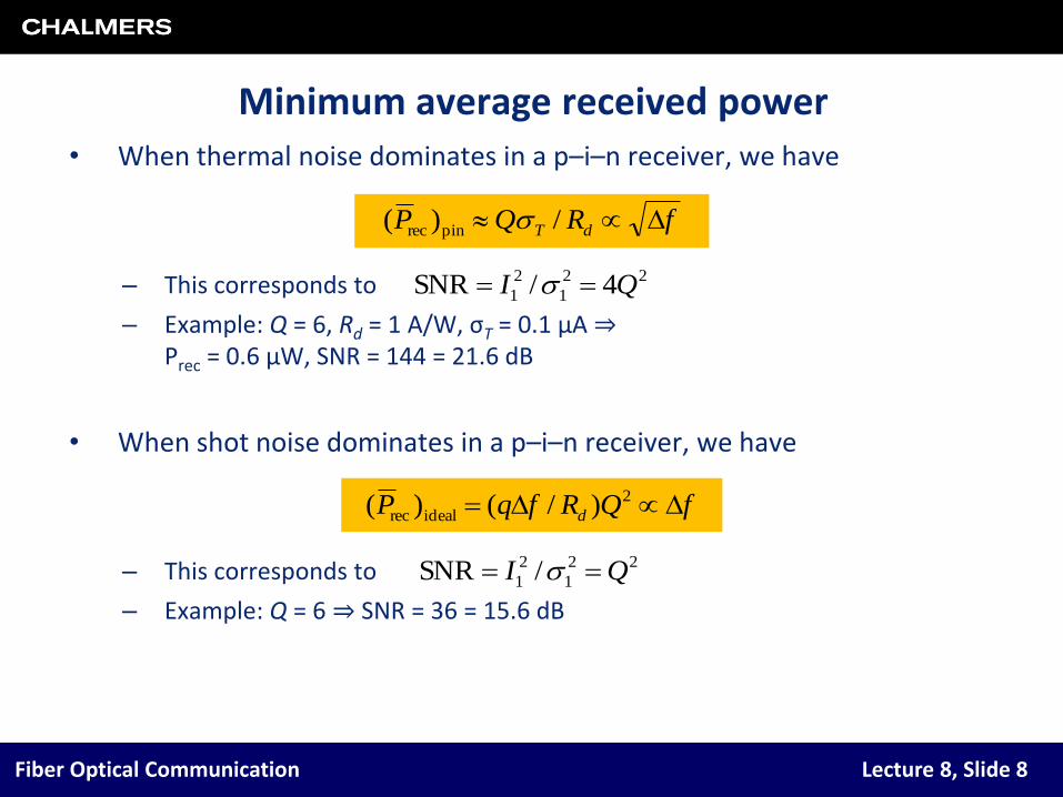
Minimum average received power• When thermal noise dominates in a p–i–n receiver, we have

– This corresponds to

– Example: Q = 6, Rd = 1 A/W, σT = 0.1 μA ⇒Prec = 0.6 μW, SNR = 144 = 21.6 dB

• When shot noise dominates in a p–i–n receiver, we have

– This corresponds to

– Example: Q = 6 ⇒ SNR = 36 = 15.6 dB

22

1

2

1 4/SNR QI

22

1

2

1 /SNR QI

fRQP dT /)( pinrec

fQRfqP d 2

idealrec )/()(


Optimum sensitivity in APD receivers• In a receiver dominated by thermal noise, an APD will increase the SNR

• There is an optimum gain, given by

• The corresponding sensitivity is

• Note: Prec Δf and not √Δf as for thermally limited receivers

• For InGaAs APDs, the sensitivity is typically improved over a p–i–n diode receiver by 6–8 dB

2/12/1

2/1

opt 1

fQqkk

fQqkM

A

TA

TA

)1()/2()( opt

2

APDrec AAd kMkQRfqP


Quantum limit of photo detection (4.6.3)• At very low power levels, the noise statistics are no longer Gaussian

• Denote the average number of photons per “one” bit by Np

• The probability of generating m electron-hole pairs is then given by the Poisson distribution

• Assume: No thermal noise, P0 = 0, threshold is at one detected photon

• For BER < 10–9, we must have Np > 20 photons per “one” bit

• This corresponds to a power in a “one” of P1 = NphνB and an average received power Prec = NphνB/2

• Example: B = 10 Gbit/s, Np=20 ⇒Prec = 13 nW at λ = 1550 nm

Poisson distribution with Np = 5

!/)exp( mNNP m

ppm

)exp()0)0()0|1()1|0(BER21

21

21

pNmpPP


Receiver characterization• Receivers are experimentally studied using a long pseudorandom

binary sequence (PRBS)

– Random data is hard to generate

– Random data is not periodic

– Typical length 215–1

• The BER is measured as a function of received average optical power

– Sensitivity = average power corresponding to a given BER (often 10–9)

PRBS generator

laser

optical attenuator

PRBS detector

decided sequence

transmitted sequence

XOR gate

receiver under test

error counter


• So far, we have discussed an ideal situation

– Perfect pulses corrupted only by (inevitable) noise

• In reality, the receiver sensitivity is degraded

– There are additional sources of signal distortion

• The corresponding necessary increase in average received power to achieve a certain BER is called the power penalty

• Also without propagation in a fiber, a power penalty can arise

• Examples of degrading phenomena include:

– Limited modulator extinction ratio

– Transmitter intensity noise

– Timing jitter

Sensitivity degradation


Extinction ratio (4.7.1)

• The extinction ratio (ER) is defined as rex = P0/P1

– P0 (P1) is the emitted power in the off (on) state

– Ideally, rex = 0

• Different for direct and external modulation

• We use that

– The average received power is Prec = (P1 + P0)/2

– The definition of the Q-parameter is Q = (I1 – I0)/(σ1 + σ0)

• We find the sensitivity degradation to be

01

2

1

1

recd

ex

ex PR

r

rQ


Extinction ratio (ER), power penalty• If thermal noise dominates, then σ1 = σ0 = σT, and the sensitivity is

• The power penalty is (in dB)

• Laser biased below threshold rex < 0.05 (–13 dB) ⇒ δex < 0.4 dB

• For a laser biased above threshold rex > 0.2 ⇒ δex > 1.5 dB

• The penalty is independent of Q and BER

• The penalty for APD receivers is larger than for p–i–n receivers

d

T

ex

exexrec

R

Q

r

rrP

1

1)(

ex

ex

rec

exrecex

r

r

P

rP

1

1log10

)0(

)(log10 1010


Intensity noise (RIN) (4.7.2)• Intensity noise in LEDs and semiconductor lasers add to the thermal and

shot noise

• Approximately, this is included by writing

where

• (The RIN spectrum was discussed earlier)

• The parameter rI is the inverse SNR of the transmitter

• Assuming zero extinction ratio and using that

we can now write the Q-value as

2222

ITs

IddI rPRPR in

2/12

in

drI )(RIN2

12

2/1

rec )4( fPqRds rec2 PRr dII

TITs

d PRQ

2/1222

rec

)(

2


Intensity noise (RIN), power penalty (4.7.3)• The receiver sensitivity is found to be

• The power penalty is

• Note that δI → ∞ when rI → 1/Q

– The receiver cannot operate at the specified BER

• A BER floor

)1()(

22

2

recQrR

fqQQrP

Id

TI

)1(log10)0(/)(log10 22

10recrec10 QrPrP III

BER Floors

Prec

BER


• The recovered clock is based on the received, noisy signal

– The decision time fluctuates and causes timing jitter

• The data is not sampled at the bit slot center

– Leads to additional fluctuations of the signal entering the decision circuit

• In a thermally limited p–i–n receiver, we have

– Δij is the current fluctuation

– σj is the corresponding RMS value

• The penalty depends on the pulse shape, but for a “typical case”

– b = (4π2/3 – 8)(Bτj)2

– τj is the RMS value of Δt

Timing jitter

time

optimal decision times

real decision times

1 01 1

TjT

jiIQ

2/122

1

)(

2/)2/1(

2/1log10

)0(

)(log10

2221010Qbb

b

P

bP

rec

recj


Timing jitter, power penalty• The power penalty depends on Q (BER)

– The penalty will be higher at a lower BER

• Rule-of-thumb:

– The RMS value of the timing jitter should typically be smaller than 5–10% of the bit slot to avoid significant penalty


Receiver performance (4.8)• Real sensitivities are

– ≈ 20 dB above the quantum limit for APDs

– ≈ 25 dB above the quantum limit for p–i–n diodes

– Mainly due to thermal noise

• Figure shows

– Measured sensitivities for p–i–n diodes (circles) and APDs (triangles)

– Lines show the quantum limit

• Two techniques to improve this

– Coherent detection

– Optical pre-amplification

– Both can reach sensitivities of only 5 dB above the quantum limit


Loss-limited lightwave systems (5.2.1)• The maximum (unamplified)

propagation distance is

– Prec is receiver sensitivity

– Ptr is transmitter average power

– αf is the net loss of the fiber, splices, and connectors

• Prec and L are bit rate dependent

• Table shows wavelengths with corresponding quantum limits and typical losses

• Loss-limited transmission

– Transmitted power = 1 mW

• λ = 850 nm, Lmax = 10–30 km

• λ = 1.55 µm, Lmax= 200–300 km

rec

trlogdB/km

10km

P

PL

f


Dispersion-limited lightwave systems (5.2.2)• Occurs when pulse broadening is

more important than loss

• The dispersion-limited distance depends on for example

– The operating wavelength

• Since D is a function of λ

– The type of fiber

• Multi-mode: step-index or graded-index

• Single-mode: standard or dispersion-shifted

– Type of laser

• Longitudinal multimode

• Longitudinal singlemode

– large or small chirp

• λ = 850 nm, multimode SI-fiber

– Modal dispersion dominates

– Disp.-limited for B > 0.3 Mbit/s

• λ = 850 nm, multimode GI-fiber

– Modal dispersion dominates

– Disp.-limited for B > 100 Mbit/s

kmMbit/s)(102 1 ncBL

kmGbit/s)(22 2

1 ncBL


• Long systems often use in-line amplifiers

– Loss is not a critical limitation

– Dispersion must be compensated for

– Noise and nonlinearities are important

– PMD can be a problem

Dispersion-limited lightwave systems• λ = 1.3 µm, SM-fiber, MM-laser

– Material dispersion dominates

– Disp.-limited for B > 1 Gbit/s

– Using |D| σλ = 2 ps/nm

• λ = 1.55 µm, SM-fiber, SM-laser


– Using |D| = 16 ps/(nm×km)


• λ = 1.55 µm, DS-fiber, SM-laser


– Using |D| = 1.6 ps/(nm×km)


kmGbit/s)(12541 DBL

kmGbit/s04001612

2

2 LB

kmGbit/s400001612

2

2 LB


• Part of the system design is to make sure the BER demand can be met

– The power budget is a very useful tool

– The transmitter average power (Ptr) and the average power required at the receiver (Prec) are often specified

– CL is the total channel loss (sum of fiber, connector, and splice losses)

– Ms is the system margin (allowing penalties and degradation over time)

• Typically Ms = 6–8 dB

• A complete system is very complex and some of the parameters that must be considered are

– Modulation format, detection scheme, operating wavelength

– Transmitter and receiver implementation, type of fiber

– The trade-off between cost and performance

– The system reliability

System design (5.2.3)

[dB][dB][dBm]

rec

[dBm]

tr sL MCPP [dB]

splice

[dB]

con

[dB/km][dB] LC fL


Computer design tools• To evaluate a complete system design, simulations are used

– VPItransmissionMaker™ is a commercial code for doing this

• Accurate modeling for many components but closed source = black box


VPItransmissionMaker™• Output will contain eye diagrams, spectra, BER etc.


Further sources of power penalty (5.4)• The above mentioned power penalties were all due to the transmitter

and the receiver

• Several more sources of power penalty appear during propagation

– Modal noise (in multi-mode fibers)

– Mode-partition noise (in multi-mode lasers)

– Intersymbol interference (ISI) due to pulse broadening

– Frequency chirp

– Reflection feedback

• All these involve dispersion


Power penalties in multi-mode fiberModal noise

• Different modes interfere over the fiber cross-section

– Forms a time-varying ”speckle” intensity pattern

– The received power will fluctuate

• Problem occurs with highly coherent sources

• To avoid this

– Use a single-mode fiber

– Reduce coherence

• Use a LED

Mode-partition noise

• The power in each longitudinal mode of a multimode laser varies with time

– Output power is constant

• Different modes propagate at different velocities in a fiber

– Additional signal fluctuation is caused and the SNR is degraded

• Negligible penalty if BLDσλ < 0.1


• Broadening affects the receiver in two ways

– Energy spreads beyond the bit slot ⇒ ISI

– Pulse peak power is reduced for a given average received power

• Reduces the SNR

• Power penalty for Gaussian pulses assuming no ISI is

• Assuming β3 ≈ C ≈ 0 and a large source spectral width, we have

Power penalty due to pulse broadening (5.4.4)

010

2

10 log100

log10

LA

Ad

2

00

1

LD 2

010 /1log5 LDd


Power penalty due to pulse broadening• Assuming β3 ≈ C ≈ 0 and a small source spectral width, we have

• Agrawal introduces the duty cycle

– A measure of the pulse width

– Defined as dc = 4 σ0/TB

• The penalty depends on

– Dispersion parameter

– Fiber length

– Bit rate

– Pulse width (duty cycle)

2

2

0

210

21log5

Ld


Power penalty due to chirp (5.4.5)• Frequency chirping increases the

impact of dispersion

• Occurs in directly modulated lasers

– Cannot modulate the amplitude without changing the phase

• Figure shows driving current, output power and wavelength of a directly modulated laser

– tc ≈ 100–200 ps = chirp duration

– Δλc = spectral shift associated with the chirp

• Exact impact is complicated

– Assume pulse is Gaussian with linear chirp


Power penalty due to chirp• For chirped Gaussian pulses with β3 ≈ 0, we have

• A chirp-free pulse (C = 0) has negligible penalty when |β2|B2L < 0.05

• Lasers have C = –4 to –8 giving δc ≈ 4–6 dB when |β2|B2L = 0.05

• A negative penalty occurs if β2C < 0 due to initial pulse compression

2

2

0

2

2

2

0

210

221log5

LLCc


Eye-closure penalty (5.4.6)• The eye is often used to monitor the signal quality

• The eye-closure penalty is

– This definition is ambiguous since ”eye opening” is not well defined

ion transmissbefore opening eye

smissionafter tran opening eyelog10 10eye

NRZ CSRZ NRZ-DPSK RZ-DPSK

0 km

263 km

eye opening


Forward error correction (FEC) (5.5)• FEC can correct errors and reduce the BER

• Redundant data is introduced

– Decreases the effective bit rate...

• With given throughput, the bit rate increases

– ...but BER is typically decreased by this operation

• Increases system complexity since encoders/decoders are needed

• Optical systems use simple FEC

– Symbol rate is very high, real-time processing is very difficult

– Reed-Solomon, RS(255, 239) is often used (gives 7% overhead)

• Coding gain is here

– Qc is Q value when using FEC

– Coding gain of 5–6 dB is obtained with modest redundancy

)/(log20 10 QQG cc


Optimum FEC• The coding gain saturates with increasing redundancy

– There is an optimal redundancy depending on system parameters

• Figure shows simulated Q values before and after FEC decoding

– WDM system, 25 channels, 40 Gbit/s per channel

– FEC increases system reach considerably

a definition of fiber optics - ttu.ee 8.pdf · · 2015-02-12fiber optical communication lecture...

Documents