A Deep Reinforcement Learning Based Multi-Criteria Decision Support System for Textile

Manufacturing Process Optimization ZHENGLEI HE KIM-PHUC TRAN SEBASTIEN THOMASSEY XIANYI ZENG

ENSAIT, GEMTEX – Laboratoire de Génie et Matériaux Textiles, F-59000 Lille, France

JIE XU, CHANGHAIYI

Wuhan Textile University, 1st, Av Yangguang, 430200, Wuhan, China

National Local Joint Engineering Laboratory for Advanced Textile Processing and Clean Production, 430200, Wuhan,

China

Textile manufacturing is a typical traditional industry involving high complexity in interconnected processes with limited capacity on

the application of modern technologies. Decision-making in this domain generally takes multiple criteria into consideration, which

usually arouses more complexity. To address this issue, the present paper proposes a decision support system that combines the

intelligent data-based models of random forest (RF) and a human knowledge-based multi-criteria structure of analytical hierarchical

process (AHP) in accordance with the objective and the subjective factors of the textile manufacturing process. More importantly, the

textile manufacturing process is described as the Markov decision process (MDP) paradigm, and a deep reinforcement learning scheme,

the Deep Q-networks (DQN), is employed to optimize it. The effectiveness of this system has been validated in a case study of

optimizing a textile ozonation process, showing that it can better master the challenging decision-making tasks in textile manufacturing

processes.

Keywords: Deep Reinforcement Learning; Deep Q-Networks; Multi-Criteria; Decision Support; Process; Textile

Manufacturing.

1. Introduction

There has been globally increasing competition in the textile industry that forces the manufacturers to

innovatively promote the product quality, process efficiency, and process environmental issues as a whole.

Compared with the other industrial sectors, textile manufacturing is a traditional sector relied on small and medium

enterprises in general and it is highly complex due to the intricate relationship involved in a large number of

parameter variables from a variety of processes[1]. It is nearly impossible to upgrade the textile manufacturing

processes directly by only following the cases from other industries without considering the detailed characteristics

of this sector and specific investigations in the applicable advanced technologies. To this end, the construction of

accurate models for simulating manufacturing processes using intelligent techniques is rather necessary[2]. However,

the decision space in a model relating to the different combinations of process and variable of textile manufacturing

can be enormous and stochastic as there are numerous factors interactively impacting the performance[3]. Therefore,

developing a decision support system to optimize the solutions in this issue remains an open challenge.

As the relationship between process parameters and product properties is not clearly known for textile

manufacturing processes, the decision-maker is unaware of the probabilities of future states, which turns out that the

present situation of decision making mostly is under uncertainty or risk[4]. By taking advantage of models learning

from data and knowledge on the basis of artificial intelligence[5], a decision support system can make a difference in

this regard. The applications of decision support systems for optimizing textile processes have been reported with

various techniques: genetic algorithm [6]and fuzzy technology [7], [8] etc. But along with the development of

artificial intelligence techniques and the growth of complexity in textile manufacturing, those classical approaches

are no longer efficient in some scenarios. This is due to the fact that in recent years, a growing number of textile

manufacturing problems were come up with large-scale data and high dimensional decision space[9], and instead of

a single standard, multi-criteria is increasingly taken into consideration in these problems as evaluating the

performance of a textile manufacturing[10].

Factors of textile manufacturing process consist of both objective and subjective effects, upon which this paper

proposes a decision support system for optimizing the textile manufacturing process by combining the intelligent

data-based models of random forest (RF) and human knowledge-based multi-criteria structure of analytical

hierarchical process (AHP). Here, the proposal of the ensemble learning approach of RF for modeling textile process

lies in the excellent approximation ability RF shown in a previous study[11] to deal with the complex and uncertain

impacts of textile process variables on its performance, whereas the application of AHP, a multi-criteria decision

making (MCDM) tool, regards to the fact that there are a few criteria govern the quality of textile process

performance and their significance with an overall objective is different. Meanwhile, concerning the growing

complexity in terms of large-scale data and high dimensional decision space in the textile manufacturing sector, this

developed system formulates the textile manufacturing process optimization problem into a Markov decision process

(MDP) paradigm and applies deep reinforcement learning (more specifically, the Deep Q-networks, DQN) instead of

current methods to collaboratively approach the optimization problems in the textile manufacturing process.

The main contributions of this paper are listed below:

(1) The uncertainties of solutions on textile manufacturing performances are driven out by the RF approach in

terms of process modeling.

(2) In terms of the widely existing MCDM problems in the field of textile, AHP is presented in this study to

cooperatively work with the aforementioned measures.

(3) Formulation of the textile manufacturing process optimization as a Markov decision process problem and

the solution based on the RL algorithm is proposed for the first time to deal with decision-making issues in

the textile industry.

(4) The application of DQN is extended to support decision making on textile manufacturing solutions.

Compared to the tabular RL algorithms applied in prior related works, DQN is more applicable and

preferred to cope with the complicated realistic problem in the textile industry.

(5) Construction of a decision support system for textile manufacturing process optimization with case

application.

The remainder of this paper is structured as follows: Section 2 summarizes relevant works. Section 3 describes

in detail the study background in terms of problem formulation and the proposed algorithms for multi-criteria

decision making in the presence of uncertainty. The detailed framework of the proposed system and a case study of

applying the system to optimize an advanced textile finishing process optimization are introduced in Section 4 and

Section 5 respectively. Finally, the discussions about future prospects and limitations are summarized in Section 6.

Section 7 concludes this paper.

2. Relevant literature

Textile manufacturing originates from the fibers (e.g. cotton) to final products (such as curtain, garment, and

composite) through a very long procedure with a wide range of different processes filled with a large number of

variables. Decision-makers should be very knowledgeable about all the processes and parameters so that a solution

of production scheme with optimal parameter setting could be provided quickly and properly from the numerous

possibilities. This is extremely challenging with a dramatically high cost and is even impossible.

The decision support system can make a difference in this issue on the basis of intelligent techniques for

modeling, optimization, and decision making. Majumdar et al. [12] briefly outlined the methods applied in the textile

industry for process modeling (linear regression, artificial neural network, and fuzzy logic), optimization (linear

programming, genetic algorithm, simulated annealing, Tabu search, and ant colony optimization) and multi-criteria

decision making (AHP, and TOPSIS i.e. technique for order preference by similarity to ideal solutions ). Regarding

the intelligent techniques, the combined use of artificial neural networks (ANN) and genetic algorithm (or evolution

algorithm) was generally the first choice that researchers applied to deal with optimization problems in the textile

domain [6], [13]–[17]. However, there are also numerous attempts were conducted on other methods, like adaptive

network-based fuzzy inference system (ANFIS)[18], support vector machine [19]–[22], and gene expression

programming [23], [24] etc. Due to the fact that the data in the textile industry is always limited for most of the

processes nowadays, and our previous study released that the random forest (RF) model can work well in this

situation compared with the extreme learning machine based ANN and SVM [11], so the RF model is proposed to

simulate the textile manufacturing process in this paper, as a part of the proposed decision support system. In terms

of the optimization techniques, it is known that the genetic algorithm and grey relational analysis [25] have been

successfully applied in many other literatures for textile process decision-making, but in industry 4.0 era, the massive

quantities of data and the high dimensional decision space of optimizing a textile manufacturing process may hinder

the application of these tools. Reinforcement learning (RL) is a machine learning approach using a well understood

and mathematically grounded framework of MDP that has been broadly applied to tackle the practical decision-

making issues in the industry. For example, the pricing optimization[26]–[30], and the production or workflow

scheduling [31], [32], as well as the energy management associated problems[33], [34]. Furthermore, using the

temporal difference based RL methods to reduce the dimension of data in feature selection has been reported by

Mehdi et al. [35] , and Jasmin et al[36] have applied the RL to approach the economic dispatch problem. Deep

reinforcement learning (DRL) is an intelligent RL based technique that can well handle the large scale data and high-

dimensional decision space. Related application of DRL for decision-making has been reported[37][38], however, at

present, there is no complete study to solve a complex production problem, especially in the textile manufacturing

industry.

As the most frequently used and widely discussed MCDM from the recently developed discipline of operation

research, AHP has been proven to be an extremely useful decision-making method in the textile industry from the

issued applications of AHP estimating the quality of fibers[39]and fabrics[40], the functional clothing design[12],

rotor spinning machine setting[10], and the maintenance strategy evaluation[41], though certain reports have come

up with their concerns on the theoretical basis of AHP[42]–[44]. The popular application and discussion of AHP in

the textile industry are owing to its involvement of both objective and subjective factors that agree with the

characteristic of the decision-making problem in the textile manufacturing process.

In summary, previous work addresses the optimization problems in the textile manufacturing process using

methods different from the ones we are proposing in this article. Their approaches were found either performed not

well relatively, or barely containing big data and high complexity. In the proposed framework, the RL would be

cooperatively applied with RF models and AHP to optimize the solutions of the textile manufacturing process

against multi-criteria.

3. Background

3.1. Problem formulation

Suggest a textile manufacturing process P involves a set of parameter variables {v1, v2… vn}, and the

performance of this process is evaluated by multi-criteria of {c1, c2… cm}. Decision making needs to figure out how

those parameter variables affect the process performances in terms of each criterion, and whether a solution of P {v1i,

v2j… vnk}is good or not relating to {c1, c2… cm}.

Suppose there is a model maps v1, v2… vn of the process to its performance in accordance with {c1, c2… cm}, then

the performance of the specific solution could be presented by:

𝑓𝑖(𝑣1, 𝑣2 … 𝑣𝑛) │ 𝑐𝑖 , 𝑓𝑜𝑟 𝑖 = 1, …𝑚 (1)

When the domain of vj ∈ Vj is known, and the multi-criteria {c1, c2… cm} problem could be somehow represented

by C, and the Equation (1) could be simplified to (2), and so that the objective of decision-makers is to find (3):

𝑓 (𝑣1, 𝑣2 … 𝑣𝑛) │ 𝐶, 𝑣𝑗 ∈ 𝑉𝑗 (2)

𝑎𝑟𝑔𝑚𝑎𝑥𝑣𝑗 ∈ 𝑉𝑗[ 𝑓 (𝑣1, 𝑣2 … 𝑣𝑛) │ 𝐶] (3)

Equation (3) aims at searching the optimal solution of variable settings, while the traditional operation in this

area usually relied heavily on trial and error.

3.2. Random forest models

The RF is a predictive model composed of a weighted combination of multiple regression trees to map the inputs

and targets by learning from data. It constructs each tree using a different bootstrap sample of the data. It is different

from the decision tree due to the splitting where each node uses the best split among all variables, by contrast, the RF

uses the best among a subset of predictors randomly chosen at that node[45]. Generally, combining multiple

regression trees increases predictive performance. It performs a prediction accurately by taking advantage of the

interaction of variables and the evaluation of the significance of each variable[46]. The RF regressor is an ensemble-

learning algorithm depending on a bagging method that combines multiple independently-constructed decision tree

predictors to classify or predict certain output variables[46]. In the RF, successive trees do not rely on earlier trees;

they are independent by using a bootstrap sample of the dataset, and therefore a simple unweighted average over the

collection of grown trees {h(x,Θk)} would be taken for prediction in the end. :

ℎ̅(𝑥) =

1

𝐾∑ ℎ(𝑥, 𝛩𝑘)

𝐾𝑘=1 (4)

where k=1,…,K is the number of trees, x represents the observed input vector, Θ is an independent identically

distributed random vector that the tree predictor takes on numerical values. RF algorithm starts from randomly

drawing ntree bootstrap samples from the original data with replacement. And then grow a certain number of

regression trees in accordance with the bootstrap samples. In each node of the regression tree, a number of the best

split (mtry) randomly selected from all variables are considered for binary partitioning. The selection of the feature

for node splitting from a random set of features decreases the correlation between different trees and thus the average

prediction of multiple regression trees is expected to have lower variance than individual regression trees[47].

Regression tree hierarchically gives specific restriction or condition and it grows from the root node to the leaf node

by splitting the data into partitions or branches according to the lowest Gini index:

𝐼𝐺(𝑡𝑋(𝑋𝑖)) = 1 − ∑ 𝑓(𝑡𝑋(𝑋𝑖)

，𝑗)2

𝑀𝐽=1 (5)

where 𝑓(𝑡𝑋(𝑋𝑖)，𝑗) is the proportion of samples with the value xi belonging to leave j as node t[48].

The application of random forest in the textile industry has been addressed to detect textile surface defects[49]

and predict the photovoltaic properties of phenothiazine dyes[50]. According to our previous research[11], RF model

was found that can well tackle the uncertainties in predict the unknown performance of different textile process

solutions, therefore this study proposed RF models to construct the proposed framework. In the RF models, variables

of the textile manufacturing process, v1, v2… vn, constitute the input, while the targets, as described in Equation(1),

are determined by the process performance against multi-criteria {c1, c2… cm}.

3.3. Analytic Hierarchy Process for Multi-criteria optimization

The multi-criteria decision making (MCDM) problem presented in Equation (3) could be summarized as a single

objective optimization problem by structuring a hierarchy of criteria in terms of weights or priorities:

𝑎𝑟𝑔𝑚𝑎𝑥𝑣𝑗 ∈ 𝑉𝑗

[ 𝑓 (𝑣1, 𝑣2 … 𝑣𝑛) │ 𝐶] = 𝑎𝑟𝑔𝑚𝑎𝑥𝑣𝑗 ∈ 𝑉𝑗∑ 𝑤𝑖𝑓𝑖(𝑣1, 𝑣2 … 𝑣𝑛)

𝑚

𝑖=1 (6)

where w1 to wm are weights of criterion c1 to cm respectively.

The AHP is a MCDM method introduced by Saaty [51] that uses a typical pair-wise comparison method to

extract relative weights of criteria and alternative scores and turns a multi-criteria problem to the paradigm of

Equation (6). Above all, it constructs a pairwise comparison matrix of attributes using a nine-point scale of relative

importance, in which number 1 denotes an attribute compared to itself or with any other attribute as important as

itself, the numbers of 2, 4, 6 and 8 indicate intermediate values between two adjacent judgments, whereas the

numbers 3, 5, 7 and 9 correspond to comparative judgments of ‘moderate importance’, ‘strong importance’, ‘very

strong importance’ and ‘absolute importance’ respectively. A typical comparison matrix (𝐶𝑚) of m × m could be

established for m criteria as demonstrated below:

𝐶𝑚 = [1 ⋯ 𝑎1𝑚

⋮ ⋱ ⋮𝑎𝑚1 ⋯ 1

] (7)

where 𝑎𝑖𝑗 represents the relative importance of criterion ci regarding criterion cj. Thus 𝑎𝑖𝑗 =1

𝑎𝑗𝑖 and 𝑎𝑖𝑗 = 1

when i = j. Note that a consistency index (CI) is introduced in AHP with consistency ratio (CR) on the basis of the

principal eigenvector (λmax) to validate the consistency in the pairwise comparison matrix:

𝐶𝐼 =

𝜆𝑚𝑎𝑥 − 𝑚

𝑚 − 1 𝑎𝑛𝑑 𝐶𝑅 =

𝐶𝐼

𝑅𝐶𝐼 (8)

where RCI is a random consistency index and the values of it are available in[42]. Afterward, the relative weight of

the ith criteria (wi) would be calculated by the geometric mean of the principal eigenvector, ith row (GMi), of the

above matrix, and then normalizing the geometric means of rows:

𝐺𝑀𝑖 = {∏𝑎𝑖𝑗

𝑚

𝑗=1

}

1𝑚

𝑎𝑛𝑑 𝑤𝑖 =𝐺𝑀𝑖

∑ 𝐺𝑀𝑖𝑚𝐼=1

(9)

3.4. The Markov decision process

Reinforcement learning (RL) is a machine learning algorithm that sorts out the Markov decision process (MDP)

in the formula of a tuple:{S, A, T, R}, where S is a set of environment states, A is a set of actions, T is a transition

function, R is a set of reward or losses. An agent in an MDP environment would learn how to take action from A by

observing the environment with states from S, according to corresponding transition probability T and reward R

achieved from the interaction. The Markov property indicates that the state transitions are only dependent on the

current state and current action is taken, but independent to all prior states and actions[52]. As known that a textile

manufacturing process has a number of parameter variables as P {v1, v2… vn}, if the probable value of vj is p(vj), the

parameter of the process defining the environment space 𝜑 from ∏ 𝑝(𝑣𝑗),𝑛𝑗=1 𝑣𝑗 ∈ 𝑉𝑗 impacting the performance of

textile process with regards to criteria {c1, c2… cm}. These parameter variables are independent to each other and obey

a Markov process that models the stochastic transitions from a state St at time step t to next state St+1, where the

environment state at time step t is:

St = [ 𝑠𝑡𝑣1 , 𝑠𝑡

𝑣2… 𝑠𝑡𝑣𝑛] ∈ 𝜑 (10)

RL trains an agent to act optimally in a given environment based on the observation of states and the feedback

from their interaction, acquiring rewards and maximizing the accumulative future rewards over time from the

interaction[52]. Here, the agent learns in the interaction with the environment by taking actions that can be conducted

on the parameter variables ∈ P {v1, v2… vn} at time step t. More specifically, in a time step t, the action of each single

variable 𝑣𝑗 could be kept (0) or changed up (+) / down (-) in the given range with specific unit uj. So there are 3n

actions totally in the action space and, for simplicity, the action vector 𝐴𝑡 at time step t could be:

𝐴𝑡 = [𝑎𝑡𝑣1 , 𝑎𝑡

𝑣2 …𝑎𝑡𝑣𝑛], where 𝑎𝑡

𝑣𝑗∈ {−𝑢𝑗 , 0, +𝑢𝑗}, 𝑣𝑗 ∈ 𝑉𝑗. (11)

The state transition probabilities, as mentions that, are only dependent on the current state St and action𝐴𝑡. It

specifies how the reinforcement agent takes action 𝐴𝑡 at time step t to transit from St to next state St+1 in terms of T

(St+1│St, 𝐴𝑡 ). For all 𝑎𝑡

𝑣𝑗∈ {−𝑢𝑗 , 0, +𝑢𝑗}, 𝑣𝑗 ∈ 𝑉𝑗 , 𝑇 (𝑆𝑡+1│𝑆𝑡 , 𝐴𝑡) > 0 and ∑ 𝑇 (𝑆𝑡+1│𝑆𝑡 , 𝐴𝑡) = 1𝑆𝑡+1∈𝜑

. The

reward achieved by an agent in an environment is specifically related to its transition between states, which evaluates

how good the transition agent conducts and facilitates the agent to converging faster to an optimal solution.

3.5. Deep-Q-network algorithm

The RL performs a vital function in the MDP problem. However, the basic RL algorithms in most of the studies,

such as the Q-learning and the SARSA (0/λ), are based on a memory-intensive tabular representation (i.e. Q-table) of

the value, or instant reward, of taking an action a in a specific state s (the Q value of state-action pair, a.k.a Q(s, a)).

The tabular algorithms would restrict the application of the RL in realistic large-scale cases when the amounts of

states or actions are tremendous. Because in these situations, not only the tables come short of recording all of the

Q(s,a), but presenting computational power would be overwhelming as well.

The deep neural networks (DNNs) is another widely applied machine learning technique that is quite good at

coping with the large-scale issues and has recently been combined with the RL to evolve toward deep reinforcement

learning (DRL). Deep-Q-network is a DRL developed by Mnih et al[53] in 2015 as the first artificial agent that is

capable of learning policies directly from high-dimensional sensory inputs and agent-environment interactions. It is

an RL algorithm proposed based on Q-learning which is one of the most widely used model-free off-policy and

value-based RL algorithms.

3.5.1. Q-learning

Q-learning learns through estimating the sum of rewards r for each state St when a particular policy π is being

performed. It uses a tabular representation of the Qπ(𝑆𝑡 , 𝐴𝑡) value to assign the discounted future reward r of state-

action pair at time step t in Q-table. The target of the agent is to maximize accumulated future rewards to reinforce

good behavior and optimize the results. In Q-learning algorithm, the maximum achievable Qπ(𝑆𝑡 , 𝐴𝑡) obeys Bellman

equation on the basis of an intuition: if the optimal value Qπ(𝑆𝑡+1, 𝐴𝑡+1) of all feasible actions 𝐴𝑡+1on state 𝑆𝑡+1 at

the next time step is known, then the optimal strategy is to select the action 𝐴𝑡+1 maximizing the expected value of

𝑟 + 𝛾 ∙ 𝑚𝑎𝑥𝐴𝑡+1𝑄π(𝑆𝑡+1, 𝐴𝑡+1).

𝑄π(𝑆𝑡 , 𝐴𝑡) = 𝑟 + 𝛾 ∙ 𝑚𝑎𝑥𝐴𝑡+1𝑄π(𝑆𝑡+1, 𝐴𝑡+1) (12)

According to the Bellman equation, the Q-value of the corresponding cell in Q-table is updated iteratively by:

𝑄π(𝑆𝑡 , 𝐴𝑡) ← 𝑄π(𝑆𝑡 , 𝐴𝑡) + 𝛼[𝑟 + 𝛾 ∙ 𝑚𝑎𝑥𝐴𝑡+1𝑄π(𝑆𝑡+1, 𝐴𝑡+1) − 𝑄π(𝑆𝑡 , 𝐴𝑡)] (13)

where 𝑆𝑡 and 𝐴𝑡 are the current state and action respectively, while 𝑆𝑡+1 is the state achieved when executing

𝐴𝑡+1 in the set of S and A in any given MDP tuples of{S, A, T, R}. 𝛼 ∊ [0, 1] is the learning rate, which indicates how

much the agent learned from new decision-making experience (𝑄π(𝑆𝑡+1, 𝐴𝑡+1)) would override the old memory

(𝑄π(𝑆𝑡 , 𝐴𝑡)). r is the immediate reward, 𝛾 ∊ [0, 1] is the discount factor determining the agent’s horizon.

The agent takes action on a state in the environment and the environment interactively transmits the agent to a

new state with a reward signal feedback. The basic principle of Q-learning RL essentially relies on a trial and error

process, but different from humans and other animals who tackle the real-world complexity with a harmonious

combination of RF and hierarchical sensory processing systems, the tabular representation of Q-learning is not

efficient at presenting an environment from high-dimensional inputs to generalize past experience to new

situations[53].

3.5.2. DQN: innovative combination of deep neural networks and Q-learning

Q-table saves the Q value of every state coupled with all its feasible actions in an environment, while the

growing complexity in the problem nowadays indicates that the states and actions in an RL environment could be

innumerable (such as Go game). In this regard, DQN applies DNNs instead of Q-table to approximate the optimal

action-value function. The DNNs feed by the state for approximating the Q-value vector of all potential actions, for

example, are trained and updated by the difference between Q-value derived from previous experience and the

discounted reward obtained from the current state. While more importantly, to deal with the instability of RL

representing the Q value using nonlinear function approximator[54], DQN innovatively proposed two ideas termed

experience replay[55] and fixed Q-target. As known that Q-learning is an off-policy RL, it can learn from the current

as well as prior states. Experience replay of DQN is a biologically inspired mechanism that learns from randomly

taken historical data for updating in each time step, which therefore would remove correlation in the observation

sequence and smooth over changes in the data distribution. Fixed Q-target performs a similar function, but

differently, it reduces the correlations between the Q-value and the target by using an iterative update that adjusts the

Q-value towards target values periodically.

Specifically, the DNNs approximate Q-value function in terms of Q-(s, a; θi) with parameters θi which denotes

weights of Q-networks at iteration i. The implementation of experience replay is to store the agent’s experiences et=

(St, At, rt, S t+1,) at each time step t in a dataset Dt = {e1,…et,}. Q-learning updates were used during learning to

samples of experience, (S, A, r, S’) ~ U(D), drawn uniformly at random from the pool of stored samples. The loss

function of Q-networks update at iteration i is:

𝐿𝑖(𝜃𝑖) = 𝔼(𝑆,𝐴,𝑟,𝑆’) ~ 𝑈(𝐷) [((𝑟 + 𝛾 ∙ 𝑚𝑎𝑥

𝐴′𝑄(𝑆′, 𝐴′; 𝜃𝑖

−) − 𝑄(𝑆, 𝐴; 𝜃𝑖))

2

] (14)

where 𝜃𝑖−are the networks weights from some previous iteration. The targets here are dependent on the network

weights; they are fixed before leaning begins. More precisely, the parameters 𝜃𝑖− from the previous iteration are fixed

as optimizing the ith loss function 𝐿𝑖(𝜃𝑖) at each stage and are only updated with 𝜃𝑖 every R steps. To implement this

mechanism, DQN uses two structurally identical but parametrically differential networks, one of it predicts

Q(𝑆, 𝐴; 𝜃𝑖) using the new parameters 𝜃𝑖, the rest one predicts 𝑟 + 𝛾 ∙ max𝐴′

𝑄(𝑆′, 𝐴′; 𝜃𝑖−) using previous parameters

𝜃𝑖− . Every R steps, the Q network would be cloned to obtain a target network �̂�, and then �̂� would be used to

generate Q-learning target 𝑟 + 𝛾 ∙ max𝐴′

𝑄(𝑆′, 𝐴′; 𝜃𝑖−) for the following R updates to network Q.

The DQN is a typical and classic DRL algorithm that played a key role in the applications of production

scheduling, playing video games, and the Computer Go [31], [53], [56], etc. Given the advantages that the DQN can

offer when confronted with decision making in textile process optimization, this algorithm would be adopted in the

construction of the proposed decision support system.

4. System framework

Figure 1 illustrates the textile manufacturing process optimization problem in the paradigm of RL, where the

decision-maker plays the role of agent to traverse and explore the state space, the environment includes all the

targeted process parameter variables, the adjustment of parameter variables indicates the action, the solution

combined of all the parameter variables represents the state, and the objective function denotes the reward. The

objective of the developed decision support system is to optimize the textile process with regards to its parameter

variables on the basis of the multi-criteria objective function which has fundamentally been formulated in

Equation(3). Therefore, here the feedback from the environment depending on a reward function is in accordance

with the objective function.

Machine learning library of Scikit-learn is employed to develop the RF models [57], where the sub-sample size

of it is always the same as the original input sample size but the samples are drawn with a replacement if bootstrap is

used (or else the whole dataset would be used to build each tree). RF algorithm starts from randomly drawing a

number of samples from the original data and grows corresponding regression trees (n_estimators) in accordance

with the drawn samples. In each leaf node of regression tree, respectively given the minimum number of samples

required to be at a leaf node (min_samples_leaf) and to split an internal node (min_samples_split) as well as the

maximum depth of the tree (max_depth), a number of the best splits (max_features) randomly selected from all

variables are considered for binary partitioning. The selection of the feature for node splitting from a random set of

features decreases the correlation between different trees and thus the average prediction of multiple regression trees

is expected to have lower variance than individual regression trees[47]. A hyperparameter tuning process using a grid

search with 3-fold cross-validation is conducted in this study for optimizing the RF models, and the applied

parameter grid with 3960 combinations is demonstrated in Table 1.

Figure 1. The MDP structure of textile manufacturing process multi-criteria optimization in the proposed framework

TABLE I. PARAMETER GRID USED IN HYPERPARAMETER TUNING PROCESS

Parameter of RF Options and implication

bootstrap True or False : sampling data points with or without replacement

n_estimators 200, 400, 600, 800, 1000, 1200, 1400, 1600, 1800, 2000

min_samples_leaf 1, 2, 4

min_samples_split 2, 5, 10

max_depth 10, 20, 30, 40, 50, 60, 70, 80, 90, 100, None

max_features ‘auto’: max_features = x (the number of observed input vector)

‘sqrt’: max_features = √𝑥

Algorithm 1: Multi-criteria decision support system main body:

Initialize: De (process experience data), 𝐶𝑚 (comparison matrix of considered criteria),

P (p1, p2 … pm, expected performance of process), E (number of episodes), N (number of time steps),

𝛼 (learning rate), 𝛾 (discount factor), R (the step updating DQN), D (replay memory size);

Phase 1: RF model construction

Split input and output of De to train and test RF models respectively;

For each output (process performance in regard to criterion 𝑐𝑖) do

RF model 𝑓𝑖(𝑣1, 𝑣2 … 𝑣𝑛) │ 𝑐𝑖 ← 𝑝𝑎𝑟𝑎𝑚𝑒𝑡𝑒𝑟 𝑡𝑢𝑛𝑖𝑛𝑔 𝑟𝑒𝑠𝑢𝑙𝑡 𝑤𝑖𝑡ℎ 𝑚𝑖𝑛 𝑒𝑟𝑟𝑜𝑟 (𝑠𝑒𝑒 𝑇𝐴𝐵𝐿𝐸 1)

End for

Phase 2: Multi-criteria summary

Initialize and check multi-criteria pairwise comparison matrix 𝐶𝑚 = [1 ⋯ 𝑎1𝑚

⋮ ⋱ ⋮𝑎𝑚1 ⋯ 1

] ;

Geometric mean 𝐺𝑀𝑖 = {∏ 𝑎𝑖𝑗𝑚𝑗=1 }

1

𝑚 and relative weight of criterion 𝑤𝑖 =𝐺𝑀𝑖

∑ 𝐺𝑀𝑖𝑚𝐼=1

;

Transformation: 𝑎𝑟𝑔𝑚𝑎𝑥𝑣𝑗 ∈ 𝑉𝑗 [ 𝑓 (𝑣1, 𝑣2 … 𝑣𝑛) │ 𝐶] = 𝑎𝑟𝑔𝑚𝑎𝑥𝑣𝑗 ∈ 𝑉𝑗

∑ 𝑤𝑖𝑓𝑖(𝑣1, 𝑣2 … 𝑣𝑛) 𝑚𝑖=1 ;

Phase 3: Optimization using DQN

Initial function 𝑄 with random weights 𝜃:

Initial function �̂� with weights 𝜃− = 𝜃;

Initialize state s0= (𝑣1, 𝑣2 … 𝑣𝑛)

For episode =1, E do

For time step=1, N do

(agent)

(Environment)

Criteria-1

Criteria-2

…

Criteria-m

Variables(v1, v2…vn)

Process performance onmulti-criteria

(reward)

Variation ofvariables

(action)

Solution

(state)

RF models

DQN

Decision maker

RF models

AHP

Choose an action at using ε-greedy policy

Execute action at , observe next state st+1

Estimate 𝑓(𝑠𝑡) and 𝑓(𝑠𝑡+1) to observe 𝑟𝑡 (𝑟𝑡 = ∑ √𝑤𝑖2(𝑓𝑖(𝑠𝑡) − 𝑝𝑖)

2𝑚𝑖=1 − ∑ √𝑤𝑖

2(𝑓𝑖(𝑠𝑡+1) − 𝑝𝑖)2𝑚

𝑖=1 )

Store transition (st, at, rt, st+1) in D

Sample random minibatch of transitions (st, at, rt, st+1) from D

Set 𝑦𝑖 = {𝑟𝑗 if terminates at step 𝑗 + 1

𝑟𝑗 + 𝛾𝑚𝑎𝑥𝑎′�̂�(𝑠𝑗+1, 𝑎′; 𝜃−) otherwise

Perform a gradient descent step on (𝑦𝑖 − 𝑄(𝑠𝑗 , 𝑎𝑗; 𝜃))2

with regard to 𝜃

Every R steps reset �̂� = 𝑄

st ← st+1

End For

End For

The pseudo-code of the proposed multi-criteria decision support system based on DQN reinforcement learning,

RF models, and AHP are illustrated in Algorithm 1, and an episodic running within the algorithm is graphically

displayed in Figure 2. Apart from the aforementioned parameters, it is also necessary to provide an experience

dataset (De) regarding the textile process modeling and the expected process performance or optimization targets (P)

to the system construction. In order to balance the exploration and exploitation of states at the learning period and

optimizing period respectively, we initialize the first state of every episode randomly from each sub-state 𝑠𝑡𝑣𝑖 where

parameter variables 𝑣𝑗 ∈ 𝑉𝑗, and more importantly, apply increasing 𝜀-greedy policy at the meantime.

Figure 2. Flowchart of the algorithm implementing the proposed deep reinforcement learning based multi-criteria

decision support system for textile manufacturing process optimization

Algorithm 2: Choose an action using 𝜀-greedy policy

Input: 𝜀𝑖𝑛𝑐𝑟𝑒𝑚𝑒𝑛𝑡 , 𝜀𝑚𝑎𝑥

(Agent)

Replay memory (D) (Environment)

…

Loss function

-networks Target networkscopy

everyR steps

(st, at)gradient descent

rt

st+1

store(st, at, rt, st+1)

st+1 = st + at

time step + 1

[0, ]

: argmaxa / 1- : random

Initialize state s0

s0

RF Processmodels

at

AHP

St+1 = [ , … ]

𝜀 ← 𝜀 + 𝜀𝑖𝑛𝑐𝑟𝑒𝑚𝑒𝑛𝑡 (0 ≤ 𝜀 ≤ 𝜀𝑚𝑎𝑥);

If random(0,1) > 𝜀

Randomly choose action at from action space

Else

Select at=argmaxa𝑄(𝑠𝑡 , 𝑎; 𝜃)

End if

In fact, the algorithm given above can work without episodes, as the target of an RL trained agent is to find the

optimized solution, in terms of state in the environment with minimum error tested by RF models and AHP

evaluations, however, the lack of exploration of the agent in an environment may cause local optimum in a single

running. So we initialize the first state randomly and introduce an episodic learning process to the agent for enlarging

the exploration and preventing local optimum. On the other hand, we apply the increasing 𝜀-greedy policy as well.

The 𝜀-greedy policy helps the agent find the best action (maximum Q value) in the present state to go to the next

state with a possibility of 𝜀 that may also randomly choose an action with a possibility of 1 − 𝜀 to get a random next

state. While, as illustrated in Algorithm 2, increasing 𝜀-greedy is employed with an increment given in each time step

from 0 until it equals to 𝜀𝑚𝑎𝑥 . This benefits the agent to explore the unexplored states without staying in the

exploitation of already experienced states of Q-networks, and plentifully exploit them when the states are traversed

enough.

5. Case study

The application of the established decision support system to a textile color fading ozonation process was

performed to evaluate the performance of the proposed framework. Color fading is an essential textile finishing

process for specific textile products such as denim to obtain a worn fashion style[17], but it conventionally was

achieved by chemical methods that have a high cost and water consumption, as well as a heavy negative impact on

the environment. Instead, ozone treatment is an advanced finishing process employing ozone gas to achieve color

faded denim without a water bath, which consequently causes less environmental issues. The complexities of this

process have been investigated in our previous works[58]–[61], and according to the experience data with 129

samples we collected from that application, the setup of the proposed framework would be attempted to solve a 4-

targets optimization problem of color fading ozonation process.

In terms of the experience dataset used to train and test RF models, it includes 4 process parameters (water-

content, temperature, pH and time) of the process and 4 process performance index known as k/s, L*, a*, and b* of the

treated fabrics. Where the k/s value indicates color depth, while L*, a*, and b* illustrate the color variation in three

dimensions (lightness, chromatic component from green to red and from blue to yellow respectively). Normally, the

color of the final textile product in line with specific k/s, L*, a*, and b* is within the acceptable tolerance of the

consumer.

5.1. Modeling color fading ozonation process using the random forest

In terms of the RF model construction, 75% of the data was divided into the training group and the rest 25% was

used to test models. In order to decrease the bias and promote the generalization of applied RF models in the system,

we have trained 4 separate models for predicting 4 outputs (k/s, L*, a*, and b*) respectively. The results of

hyperparameter tuning in regards with the context given in Table 1 are displayed in Table 2, and the final optimized

models are tested (25% with unseen data) that can well predict the process performance with accuracies (R-square)

of 0.996, 0.954, 0.937 and 0.965 respectively.

TABLE II. THE RF MODELS HYPERPARAMETER TUNING RESULT AND THE TESTING RESULTS OF OPTIMIZED MODEL

Bootstrap n_ Min_ Min_ Max_ Max_ R2 MAE MAPE

estimators samples_

leaf

samples_

split

depth eatures

k/s True 2000 1 2 30 ‘auto’ 0.996 0.28 12.36

L* False 2000 1 2 None ‘sqrt’ 0.954 0.77 8.99

a* False 2000 2 2 None ‘auto’ 0.937 2.29 15.43

b* True 2000 1 5 100 ‘auto’ 0.965 2.87 11.62

TABLE III. PAIRWISE COMPARISON MATRIX OF K/S, L*, A* AND B* WITH RESPECT TO THE OVERALL COLOR PERFORMANCE

k/s L* a* b* GM w

k/s 1 3 5 5 2.9428 0.556

L* 1/3 1 3 3 1.3161 0.249

a* 1/5 1/3 1 2 0.6043 0.114

b* 1/5 1/3 1/2 1 0.4273 0.081

5.2. Determining the criteria weights using the analytic hierarchy process

By means of combining experts’ judgment with our experience, a pairwise comparison matrix of the 4 decision

criteria with respect to the overall color performance of ozonation process treated textile product is provided in Table

3. λmax of this comparison matrix is 4.1042 and known that the RCI for 4 criteria problem is 0.90, as a result, the CR

calculated is 0.0386≤0.08 which implies that the evaluation within the matrix is acceptable.

5.3. Deep Q-Networks for optimal decision-making

We optimize the color performance in terms of k/s, L*, a*, and b* of the textile in ozonation process by finding a

solution including proper parameter variables of water-content, temperature, pH and treating time that minimizes the

difference between such specific process treated textile product and the targeted sample. Therefore, the state space 𝜑

in this case is composed by the solutions with four parameters (water-content, temperature, pH and treating time) in

terms of St = [ 𝑠𝑡𝑣1 , 𝑠𝑡

𝑣2 , 𝑠𝑡𝑣3 , 𝑠𝑡

𝑣4]. In a time step t, the adjustable units of these parameter variables are 50, 10, 1 and 1

respectively in the range of [0, 150], [0,100], [1, 14] and [1, 60] respectively. As the action of a single variable 𝑣𝑗

could be kept (0) or changed up (+) / down (-) in the given range with specific unit u, so there are 34 =81 actions

totally in the action space and the action vector at time step t is 𝐴𝑡 = [𝑎𝑡𝑣1 , 𝑎𝑡

𝑣2 , 𝑎𝑡𝑣3 , 𝑎𝑡

𝑣4] , where 𝑎𝑡𝑣1 ∈

{−50, 0, +50}, 𝑣1 ∈ [0, 150] ; 𝑎𝑡𝑣2 ∈ {−10, 0, +10}, 𝑣2 ∈ [0, 100] ; 𝑎𝑡

𝑣3 ∈ {−1, 0, +1}, 𝑣3 ∈ [1, 14] ; 𝑎𝑡𝑣4 ∈

{−1, 0, +1}, 𝑣4 ∈ [1, 60].

The transition probability is 1for the states in the given range of state space above, but 0 for the states out of it.

The reward r at time step t is expected to be in line with how close the agent gets to our target, and as the relative

importance of these four performance criteria (0.556, 0.249, 0.114 and 0.081 respectively) is analyzed in AHP, we

could set up the reward function as illustrated below to induce the agent to approach our optimization results:

𝑟𝑡 = ∑ √𝑤𝑖

2(𝑓𝑖(𝑠𝑡) − 𝑝𝑖)2

𝑚

𝑖=1− ∑ √𝑤𝑖

2(𝑓𝑖(𝑠𝑡+1) − 𝑝𝑖)2

𝑚

𝑖=1 (15)

As shown the pseudo-code of DQN main body in Algorithm 1, optimization targets of textile ozonation process

are needed to function the system ( 𝑝1, 𝑝2, 𝑝3 , 𝑝4, the color performance of the ozonation process in terms of k/s, L*,

a*, and b*), these targets in the present case study would be sampled by experts. In addition to the targets, the

parameters of DQN such as step R for updating Q-networks and replay memory size D, as well as the learning rate 𝛼

and the discount rate 𝛾 for updating loss function, etc., are listed in Table 4. In particular, the R step for updating

DQN here denotes that after 100 steps, the Q-networks would be updated at every 5 steps.

TABLE IV. DQN ALGORITHM SETTING IN TEXTILE OZONATION PROCESS CASE STUDY

R D 𝛼 𝛾 𝜀𝑖𝑛𝑐𝑟𝑒𝑚𝑒𝑛𝑡 𝜀𝑚𝑎𝑥 E N

5(>100) 2000 0.01 0.9 0.001 0.9 5 5000

5.4. Results and discussion

As mentioned that there are four RF models trained for predicting 𝑝1, 𝑝2, 𝑝3, 𝑝4 of the color performance of the

ozonation process in terms of k/s, L*, a* and b*, respectively. The predictive performance of these models displayed

in Figure 3 clearly indicates that the models work steadily in the algorithm of present case study as it is found that

the models predicted values are generally in accordance with the actual measured values through the predictive

errors of different models varied slightly at different levels. This finding furthermore reflects that the RF approach is

capable of modeling the textile manufacturing process and plays a significant role in our proposed decision support

system. It is worth remarking that the average error of MAPE is higher than 10%. This is due to the fact that the

targets in these models, i.e. k/s, L*, a*, and b*, are the colorimetric values ranging from -120 to 120, while the sample

data applied are close to 0 and mostly are negative, which exaggerated the evaluation of MAPE in this issue.

In particular, the neural networks implemented by TensorFlow[62] are used in our case study to realize Q-

networks which have been described in detail in the developed framework of Algorithm 1. The networks consist of

two layers with 50 and 34 hidden nodes respectively, where the last layer corresponds to the actions. As demonstrated

in Table 5, there are 5 experimental targets sampled by experts that were used in the present case study.

Figure 3. Predictive performance of the RF models trained in the case study for supporting decision making in textile

color ozonation process

TABLE V. THE EXPERIMENTAL TARGETS SAMPLED BY EXPERTS WE USED IN THE CASE STUDY APPLICATION OF PROPOSED DECISION

SUPPORT SYSTEM

1 2 3 4 5

k/s 0.81 1.00 2.45 1.84 0.41

L* 15.76 11.63 8.2 9.72 21.6

a* -20.84 -24.08 -18.73 -21.09 -36.48

b* -70.79 -54.1 -38.17 -42.78 -59.95

0 1000 2000 3000 4000 5000

0

50

100

Loss

Iteration

1

2

3

4

5

10, 20, 30, 40 units of loss are

added to the curves 2, 3, 4, 5

respectively in this Figure for

illustration.

Figure 4. The loss function of target networks for each

scenario with different targets

1 2 3 4 5

0

500

1000

1500

2000

Num

ber

of

state

s explo

red

Scenarios

episode5

episode4

episode3

episode2

episode1

Figure 5. The number of states explored by the DQN agent

in each episode for different scenarios

0 1000 2000 3000 4000 5000

0

2

4

6

8

10

Min

imum

err

or

Steps

1

2

3

4

5

Figure 6. The minimum error of solutions that DQN agent has achieved along with the time steps

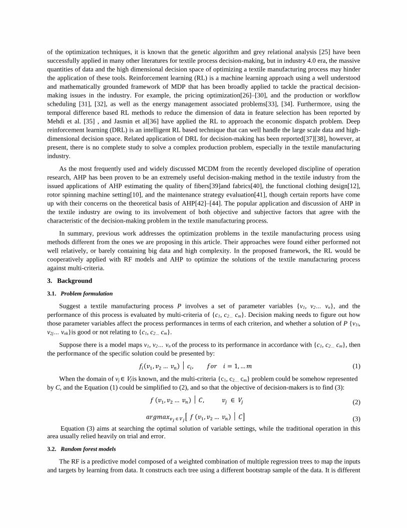
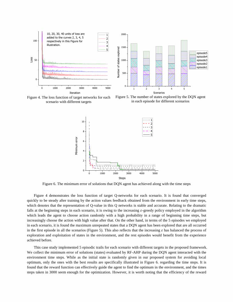
Figure 4 demonstrates the loss function of target Q-networks for each scenario. It is found that converged

quickly to be steady after training by the action values feedback obtained from the environment in early time steps,

which denotes that the representation of Q-value in this Q networks is stable and accurate. Relating to the dramatic

falls at the beginning steps in each scenario, it is owing to the increasing 𝜀-greedy policy employed in the algorithm

which leads the agent to choose action randomly with a high probability in a range of beginning time steps, but

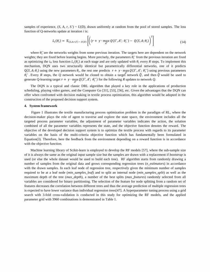
increasingly choose the action with high value after that. On the other hand, in terms of the 5 episodes we employed

in each scenario, it is found the maximum unrepeated states that a DQN agent has been explored that are all occurred

in the first episode in all the scenarios (Figure 5). This also reflects that the increasing 𝜀 has balanced the process of

exploration and exploitation of states in the environment, and the rest episodes would benefit from the experience

achieved before.

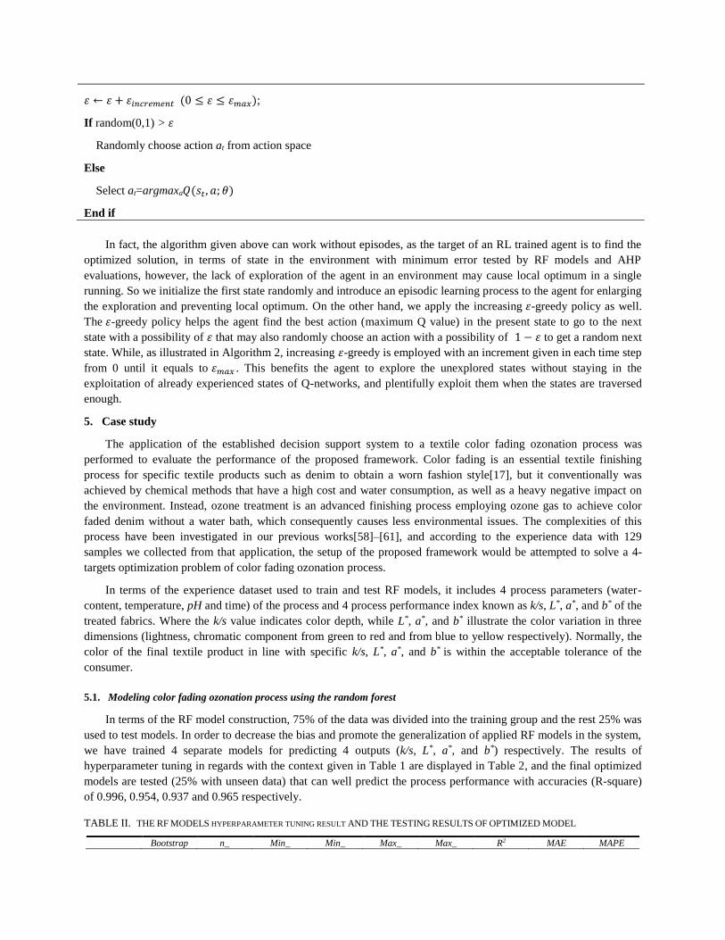
This case study implemented 5 episodic trails for each scenario with different targets in the proposed framework.

We collect the minimum error of solutions (states) evaluated by RF-AHP during the DQN agent interacted with the

environment time steps. While as the initial state is randomly given in our proposed system for avoiding local

optimum, only the ones with the best results are specifically illustrated in Figure 6. regarding the time steps. It is

found that the reward function can effectively guide the agent to find the optimum in the environment, and the times

steps taken in 3000 seem enough for the optimization. However, it is worth noting that the efficiency of the reward

function in our proposed decision support system is still not fully illustrated by this case study. One main reason for

this comes to the limited data of textile manufacturing processes and the costly computational power which

hopefully would be solved in the Industry 4.0 era.

TABLE VI. SIMULATED RESULTS OF SOLUTIONS WITH MINIMUM ERRORS OBTAINED FROM DQN BASED AND Q-LEANRING BASED FRAMEWORK

RESPECTIVELY

1 2 3 4 5

DQN

Targets

Q-

learning

In order to show the advantage and effectiveness of DQN in our proposed decision support system, a

comparison with Q-learning based on the same developed framework is conducted, and the simulated color

performance of the results in terms of the solutions with minimum error obtained from two methods are

comparatively demonstrated in Table 6 with the targets. Here the error is calculated by Equation (16), which are 1.06,

0.50, 0.88, 0.29, 0.22 and 1.13, 0.54, 0.91, 1.28, 1.76 in the DQN and Q-learning based decision support system for

scenarios from 1 to 5 respectively.

𝑒𝑟𝑟𝑜𝑟 = √0.5562(𝑘/𝑠𝑠 − 𝑘/𝑠𝑡)

2 + 0.2492(𝐿𝑠∗ − 𝐿𝑡

∗)2+0.1142(𝑎𝑠∗ − 𝑎𝑡

∗)2 + 0.0812(𝑏𝑠∗ − 𝑏𝑡

∗)2 (16)

where 𝒌/𝒔𝒔 , 𝑳𝒔∗ , 𝒂𝒔

∗ , 𝒃𝒔∗ are the properties of simulated color performance of solution obtained from the decision support

system, and 𝒌/𝒔 , 𝑳 ∗ , 𝒂

∗ , 𝒃 ∗ are the targeted color performance.

6. Limitation and future prospective

The proposed decision support system is clearly applicable in the textile manufacturing sector, which has been

tested in the implemented case study. It is worth mentioning that this system can also be applied in practice with

different objective functions such as energy optimization, material optimization, etc. However, it is worth remarking

that certain features of this framework may hinder the massive promotion and application of it. The AHP performs

well in the MCDM problems, while it relies heavily on experts’ estimation, which may limit its application in certain

areas[63], [64]. Meanwhile, it is well known that the practice and effectiveness of RF and DQN rely strongly on big

data and computation power, which is quite limited in the application of the textile industry nowadays. But the

application of artificial intelligent techniques is growing in the textile manufacturing industry, such concerns could

be properly addressed in the industry 4.0 era when it is able to take full advantage of the Internet of Things (IoT)

environment. Future development of the proposed decision support system should be able to learn from the

interaction with the complexity-growing environment online by constantly feeding new data and scenarios to follow

the development of the textile manufacturing process. Future research should devote more effort to test the proposed

framework and broaden the application of it in more textile manufacturing processes by collecting real empirical data

and construct the corresponding MDP paradigm.

7. Conclusions

Textile manufacturing is a traditional industry involving high complexities in interconnected processes with

limited capacity on the application of modern technologies. Decision-making in this domain generally takes multiple

criteria into consideration, which usually arouses more complexity. Traditional classical approaches are no longer

efficient owing to the growing complexity with large-scale data and high dimensional decision space in some

scenarios. In this paper, a decision support system combining the random forest model, analytical hierarchy process

and deep Q-Networks is proposed for optimizing the textile manufacturing process. This developed system tackles

large scale optimization problems in high dimensional decision space with multi-criteria in the textile manufacturing

process. Empirical data and human knowledge of the textile process are needed to build random forest models and

evaluate criteria respectively. The dependence of the operations on data and knowledge of this system are in

accordance with the characteristics of the complicated textile manufacturing process with respect to both objective

and subjective factors in decision making of an application. This system describes decision making for optimizing

the textile manufacturing process in the Markov decision process paradigm of {S, A, T, R} in the proposed algorithm,

and takes advantage of the deep reinforcement learning by means of a deep Q-Networks algorithm in this proposed

framework to exploit the data on the basis of random forest models and AHP multi-criteria structure to find the

optimal textile manufacturing. The application in optimizing a textile ozonation process was released. The results

showed that the developed system is capable of learning to master the challenging decision-making tasks and

performed better than traditional methods.

Acknowledgments

This research was supported by the funds from National Key R&D Program of China (Project NO:

2019YFB1706300), and Scientific Research Project of Hubei Provincial Department of Education, China (Project

NO: Q20191707).

The first author would like to express his gratitude to China Scholarship Council for supporting this study (CSC,

Project NO. 201708420166).

References

[1] A. Hasanbeigi and L. Price, “A review of energy use and energy efficiency technologies for the textile industry,” Renew.

Sustain. Energy Rev., vol. 16, no. 6, pp. 3648–3665, 2012.

[2] K. Suzuki, ARTIFICIAL NEURAL NETWORKS - INDUSTRIAL AND CONTROL ENGINEERING APPLICATIONS.

2011.

[3] J. Etters, “Advances in indigo dyeing: implications for the dyer, apparel manufacturer and environment,” Text. Chem.

Color., vol. 27, no. 2, pp. 17–22, 1995.

[4] A. Ghosh, P. Mal, and A. Majumdar, Advanced Optimization and Decision-Making Techniques in Textile Manufacturing.

2019.

[5] D. J. Power, “Decision support systems: a historical overview,” in Handbook on decision support systems 1, Springer,

2008, pp. 121–140.

[6] S. Das, A. Ghosh, A. Majumdar, and D. Banerjee, “Yarn Engineering Using Hybrid Artificial Neural Network-Genetic

Algorithm Model,” Fibers Polym., vol. 14, no. 7, pp. 1220–1226, 2013.

[7] F. Fayala, H. Alibi, A. Jemni, and X. Zeng, “Study the effect of operating parameters and intrinsic features of yarn and

fabric on thermal conductivity of stretch knitted fabrics using artificial intelligence system,” Fibers Polym., vol. 15, no. 4,

pp. 855–864, 2014.

[8] X. Zeng, L. Koehl, M. Sanoun, M. A. Bueno, and M. Renner, “Integration of human knowledge and measured data for

optimization of fabric hand,” Int. J. Gen. Syst., vol. 33, no. 2–3, pp. 243–258, 2004.

[9] Y. Xu, S. Thomassey, and X. Zeng, “AI for Apparel Manufacturing in Big Data Era: A Focus on Cutting and Sewing,” in

Artificial Intelligence for Fashion Industry in the Big Data Era, Springer, 2018, pp. 125–151.

[10] S. Kaplan, “A Multicriteria Decision Aid Approach on Navel Selection Problem for Rotor Spinning Abstract,” vol. 76,

no. 12, pp. 896–904, 2006.

[11] Z. He, K. p Tran, X. Zeng, J. Xu, and C. Yi, “Modeling color fading ozonation of reactive-dyed cotton using the Extreme

Learning Machine , Support Vector Regression and Random Forest,” Text. Res. J., vol. 90, no. 7–8, pp. 896–908, 2020.

[12] A. Majumdar, S. P. Singh, and A. Ghosh, “Modelling , optimization and decision making techniques in designing of

functional clothing,” vol. 36, no. December, pp. 398–409, 2011.

[13] S. Sette, L. Boullart, L. Van Langenhove, and P. Kiekens, “Optimizing the Fiber-to-Yarn Production Process with a

Combined Neural Network/Genetic Algorithm Approach,” Text. Res. J., vol. 67, no. 2, pp. 84–92, 1997.

[14] J. I. Mwasiagi, X. Huang, and X. Wang, “The Use of Hybrid Algorithms to Improve the Performance of Yarn Parameters

Prediction Models,” Fibers Polym., vol. 13, no. 9, pp. 1201–1208, 2012.

[15] A. Majumdar, A. Das, P. Hatua, and A. Ghosh, “Optimization of woven fabric parameters for ultraviolet radiation

protection and comfort using artificial neural network and genetic algorithm,” Neural Comput. Appl., no. October, 2016.

[16] L. Zheng, B. Du, J. Xing, and S. Gao, “Bio ‐ degumming optimization parameters of kenaf based on a neural network

model,” J. Text. Inst., vol. 101, no. 12, pp. 1075–1079, 2010.

[17] J. Xu, Z. He, S. Li, and W. Ke, “Production cost optimization of enzyme washing for indigo dyed cotton denim by

combining Kriging surrogate with differential evolution algorithm,” 2020.

[18] P. Khude and A. Majumdar, “Modelling and prediction of antibacterial activity of knitted fabrics made from silver

nanocomposite fibres using soft computing approaches,” Neural Comput. Appl., vol. 8, 2019.

[19] A. Ghosh and P. Chatterjee, “Prediction of cotton yarn properties using support vector machine,” Fibers Polym., vol. 11,

no. 1, pp. 84–88, 2010.

[20] A. Ghosh, “Forecasting of Cotton Yarn Properties Using Intelligent Machines Forecasting of Cotton Yarn Properties

Using Intelligent Machines,” Res. J. Text. Appar., vol. 14, no. 3, pp. 55–61, 2014.

[21] E. C. Doran and C. Sahin, “The prediction of quality characteristics of cotton / elastane core yarn using artificial neural

networks and support vector machines,” Text. Res. J., vol. 0, no. 0, pp. 1–23, 2019.

[22] J. Yang, Z. Lu, and B. Li, “Quality Prediction in Complex Industrial Process with Support Vector Machine and Genetic

Algorithm Optimization : A Case Study,” Appl. Mech. Mater., vol. 232, pp. 603–608, 2012.

[23] M. Dayik, “Prediction of Yarn Properties Using Evaluation Programing,” Text. Res. J., vol. 79, no. 11, pp. 963–972,

2009.

[24] A. Moghassem, A. Fallahpour, and M. Shanbeh, “An Intelligent Model to Predict Breaking Strength of Rotor Spun

Yarns Using Gene Expression Programming,” J. Eng. Fiber. Fabr., vol. 7, no. 2, 2012.

[25] S. Chakraborty, P. Chatterjee, and P. Protim, “Cotton Fabric Selection Using a Grey Fuzzy Relational Analysis

Approach,” J. Inst. Eng. Ser. E, no. Mcdm, 2018.

[26] V. Nanduri, S. Member, and T. K. Das, “A Reinforcement Learning Model to Assess Market Power Under Auction-

Based Energy Pricing,” vol. 22, no. 1, pp. 85–95, 2007.

[27] E. Krasheninnikova, J. García, R. Maestre, and F. Fernández, “Reinforcement learning for pricing strategy optimization

in the insurance,” Eng. Appl. Artif. Intell., vol. 80, no. May 2018, pp. 8–19, 2019.

[28] Y. A. Chizhov and A. N. Borisov, “Markov Decision Process in the Problem of Dynamic Pricing Policy,” vol. 45, no. 6,

pp. 361–371, 2011.

[29] R. Lu, S. H. Hong, and X. Zhang, “A Dynamic pricing demand response algorithm for smart grid : Reinforcement

learning approach,” Appl. Energy, vol. 220, no. November 2017, pp. 220–230, 2018.

[30] R. Rana and F. S. Oliveira, “Dynamic pricing policies for interdependent perishable products or services using

reinforcement learning,” Expert Syst. Appl., vol. 42, no. 1, pp. 426–436, 2015.

[31] B. Waschneck, T. Altenm, T. Bauernhansl, A. Knapp, and A. Kyek, “Optimization of global production scheduling with

deep reinforcement learning,” 2018.

[32] Y. Wei, D. Kudenko, S. Liu, L. Pan, L. Wu, and X. Meng, A Reinforcement Learning Based Workflow Application

Scheduling Approach in Dynamic Cloud Environment : 13th International Conference , A Reinforcement Learning Based

Work fl ow Application Scheduling Approach in Dynamic Cloud Environment, no. June. Springer International

Publishing, 2019.

[33] R. Rocchetta, L. Bellani, M. Compare, E. Zio, and E. Patelli, “A reinforcement learning framework for optimal operation

and maintenance of power grids,” Appl. Energy, vol. 241, no. February, pp. 291–301, 2019.

[34] E. Kuznetsova, Y. Li, C. Ruiz, E. Zio, G. Ault, and K. Bell, “Reinforcement learning for microgrid energy management,”

Energy, vol. 59, pp. 133–146, 2013.

[35] S. Mehdi, H. Fard, A. Hamzeh, and S. Hashemi, “Using reinforcement learning to find an optimal set of features,”

Comput. Math. with Appl., vol. 66, no. 10, pp. 1892–1904, 2013.

[36] E. A. Jasmin and G. E. College, “Reinforcement Learning solution for Unit Commitment Problem through pursuit

method,” no. May 2016, 2009.

[37] C.-J. Hoel, K. Wolff, and L. Laine, “Automated speed and lane change decision making using deep reinforcement

learning,” in 2018 21st International Conference on Intelligent Transportation Systems (ITSC), 2018, pp. 2148–2155.

[38] M. Mukadam, A. Cosgun, A. Nakhaei, and K. Fujimura, “Tactical decision making for lane changing with deep

reinforcement learning,” 2017.

[39] A. Majumdar, B. Sarkar, and P. K. Majumdar, “Determination of quality value of cotton fibre using hybrid AHP-

TOPSIS method of multi-criteria decision- making,” J. Text. Inst., vol. 96, no. 5, pp. 303–309, 2005.

[40] A. Mitra, A. Majumdar, A. Ghosh, and P. K. Majumdar, “Selection of Handloom Fabrics for Summer Clothing Using

Multi-Criteria Decision Making Techniques,” J. Nat. Fibers, vol. 12, pp. 61–71, 2015.

[41] K. Shyjith, M. Ilangkumaran, and S. Kumanan, “approach to evaluate optimum maintenance strategy in textile industry,”

vol. 14, no. 4, pp. 375–386, 2008.

[42] T. L. Saaty, “How to make a decision: the analytic hierarchy process,” Eur. J. Oper. Res., vol. 48, no. 1, pp. 9–26, 1990.

[43] J. S. Dyer, “Remarks on the analytic hierarchy process,” Manage. Sci., vol. 36, no. 3, pp. 249–258, 1990.

[44] E. Triantaphyllou and S. H. Mann, “A computational evaluation of the original and revised analytic hierarchy process,”

Comput. Ind. Eng., vol. 26, no. 3, pp. 609–618, 1994.

[45] A. Liaw and M. Wiener, “Classification and Regression by randomForest,” R news, vol. 2, no. December, pp. 18–22,

2002.

[46] L. Breiman, “RANDOM FORESTS,” pp. 1–33, 2001.

[47] A. Liaw and M. Wiener, “Classification and regression by randomForest,” R news, vol. 2, no. 3, pp. 18–22, 2002.

[48] L. Breiman, Classification and regression trees. Routledge, 2017.

[49] B. K. Kwon, J. S. Won, and D. J. Kang, “Fast defect detection for various types of surfaces using random forest with

VOV features,” Int. J. Precis. Eng. Manuf., vol. 16, no. 5, pp. 965–970, 2015.

[50] V. Venkatraman and B. K. Alsberg, “A quantitative structure-property relationship study of the photovoltaic

performance of phenothiazine dyes,” Dye. Pigment., vol. 114, no. C, pp. 69–77, 2015.

[51] T. L. Saaty, “What is the analytic hierarchy process?,” in Mathematical models for decision support, Springer, 1988, pp.

109–121.

[52] R. S. Sutton and A. G. Barto, Introduction to reinforcement learning, vol. 135. MIT press Cambridge, 1998.

[53] V. Mnih et al., “Human-level control through deep reinforcement learning,” Nature, vol. 518, no. 7540, pp. 529–533,

2015.

[54] J. N. Tsitsiklis and B. Van Roy, “An analysis of temporal-difference learning with function approximationTechnical,”

Rep. LIDS-P-2322). Lab. Inf. Decis. Syst. Massachusetts Inst. Technol. Tech. Rep., 1996.

[55] L.-J. Lin, “Reinforcement learning for robots using neural networks,” Carnegie-Mellon Univ Pittsburgh PA School of

Computer Science, 1993.

[56] V. Mnih et al., “Playing atari with deep reinforcement learning,” arXiv Prepr. arXiv1312.5602, 2013.

[57] F. Pedregosa, R. Weiss, and M. Brucher, “Scikit-learn : Machine Learning in Python,” vol. 12, pp. 2825–2830, 2011.

[58] Z. He, K. Tran, X. Zeng, and J. Xu, “Modeling color fading ozonation of reactive-dyed cotton using the Extreme

Learning Machine , Support Vector Regression and Random Forest,” 2019.

[59] Z. He, M. Li, D. Zuo, and C. Yi, “Color fading of reactive-dyed cotton using UV-assisted ozonation,” Ozone Sci. Eng.,

vol. 41, no. 1, pp. 60–68, 2019.

[60] Z. He, M. Li, D. Zuo, and C. Yi, “The effect of denim color fading ozonation on yarns,” Ozone Sci. Eng., vol. 40, no. 5,

2018.

[61] Z. He, M. Li, D. Zuo, J. Xu, and C. Yi, “Effects of color fading ozonation on the color yield of reactive-dyed cotton,”

Dye. Pigment., vol. 164, 2019.

[62] A. Agarwal et al., “TensorFlow : Large-Scale Machine Learning on Heterogeneous Distributed Systems,” 2015.

[63] V. Belton, “A comparison of the analytic hierarchy process and a simple multi-attribute value function,” Eur. J. Oper.

Res., vol. 26, no. 1, pp. 7–21, 1986.

[64] B. Roy, Multicriteria methodology for decision aiding, vol. 12. Springer Science & Business Media, 2013.