a decade of trace gas measurements using doas in finnish lapland

BOREAL ENVIRONMENT RESEARCH 8: 351–363 ISSN 1239-6095Helsinki 10 December 2003 © 2003

A decade of trace gas measurements using DOAS in Finnish Lapland

Aki Virkkula1), Kimmo Teinilä1), Risto Hillamo1) and Andreas Stohl2)

1) Finnish Meteorological Institute, Air Quality Research, Sahaajankatu 20 E, FIN-00880 Helsinki, Finland

2) Department of Ecology, Technical University Munich, D-85354 Freising-Weihenstephan, Germany

Virkkula, A., Teinilä, K., Hillamo, R. & Stohl, A. 2003: A decade of trace gas measurements using DOAS in Finnish Lapland. Boreal Env. Res. 8: 351–363. ISSN 1239-6095

Trace gas concentrations have been measured at Sevettijärvi in Finnish Lapland from 8 January 1992 to 10 July 2002. The maximum hourly SO

2 concentrations decreased

from around 500 µg m–3 in the fi rst two years of the monitoring to 200–300 µg m–3 in the mid 1990s. The annual average SO

2 concentrations decreased from about 5 µg m–3

to 3–4 µg m–3 during the same period when taking into account the years for which the data coverage was above 85%. For NO

2 and O

3 no clear trends were observed. The

sources of all three trace gases were investigated using wind measurements and in the case of NO

2 also using back trajectories. The analysis indicated that the source areas of

NO2 and SO

2 are to the east and north-east of the site, i.e., at Nikel-Zapolyarnyj indus-

trial areas in Kola Peninsula, Russia. In addition to these, NO2 transported from other

industrial and urban areas in Europe can also be observed at Sevettijärvi.

Introduction

At the end of the 1980s and beginning of the 1990s Finns were seriously concerned about whether the Ni-Cu smelters in the Kola Peninsula, especially at Nikel and Zapolyarnyj, could have serious effects on the nature of Finnish Lapland. There was a good reason to be concerned because these two smelters emitted more than twice the amount of SO

2 emitted by the whole of Finland (Tuovinen

et al. 1993) and because they are located close to Finnish territory. In addition in Monchegorsk, somewhat further from the Finnish border, there is another big smelter that affects Lapland. In summer 1991 the Finnish Meteorological Insti-

tute (FMI) built a station for measuring atmo-spheric aerosols and trace gases at Sevettijärvi (69°35´N, 28°50´E, 130 m above sea level) in order to study pollution coming from the Russian industrial areas in the Kola Peninsula to Finnish Lapland. The goal was to provide information on air quality for The Lapland Forest Damage Project, a multidisciplinary effort to determine the effects of Kola emissions on the health of the forests in Lapland (Tikkanen and Niemelä, 1995; www.metla.fi /julkaisut/muut/elproj/). The site is essentially as near to the large pollution sources in Kola Peninsula as possible in Finland (Fig. 1). The distance to Nikel is approximately 60 km. The site is also close to the Barents Sea

352 Virkkula et al. • BOREAL ENV. RES. Vol. 8

which is a part of the Arctic Ocean. The distance to the nearest fjord is approximately 40 km. The nearest important population centres are Kirkenes in Norway and Ivalo in Finland.

In addition to investigating fresh pollution from the Russian smelters, the site can be used to study other sources as well. As shown by Virk-kula et al. (1995, 1997, 1999), the site is exposed to air coming from sources other than the Kola Peninsula for most of the time. Pollution epi-sodes from the Kola Peninsula arrive typically at Sevettijärvi two or three times per month, while the rest of the time either continental air masses from other parts of Europe or cleaner air from the North Atlantic and Arctic Ocean arrive at the site. The most frequent wind sectors S and SW bring air from continental Europe, so the site gives a good description of the polluted Euro-pean air that leaves the continent and goes into Arctic areas. A signifi cant fraction of time the air is coming from the Norwegian Sea and the Arctic Ocean, so data on background concentrations is obtained as well. The fact that the site is north of the Arctic Circle makes it possible to investigate the effects of polar night and polar sunrise. An example of this is the relation between the SO

2

and particle number concentration, being clearly different between the dark winter months and spring/summer period (Virkkula et al. 1997). This relation has demonstrated that a large frac-tion of the aerosol observed during pollution epi-sodes from Nikel is of secondary origin. Studies on aerosol chemistry at Sevettijärvi have been presented, e.g., by Kerminen et al. (1997, 1999), Maenhaut et al. (1999a, 1999b), Fridlind et al. (2000) and Ricard et al. (2002a, 2002b).

In Norway there are measurement stations closer to the smelters. The Norwegian Institute for Air Research (NILU) has measured air pol-lution in the border areas of Norway and Russia and studied the dispersion of both gaseous and particulate air pollutants from Nikel and Zapolyarnyj for over a decade. The Norwegian results have been published regularly and exten-sively in several annual reports. In a recent report describing the results from the border stations it was shown that after a clear decrease of SO

2 con-

centrations from the 1980s to 1990s, the average concentrations have remained approximately at the same level (Hagen et al. 2002).

The aim of this paper is to investigate how the concentrations of SO

2, NO

2 and O

3 have varied

during the decade of measurements, and whether there are any trends in the peak and average concentrations of these compounds. Virkkula et al. (1995, 1997) presented a source analysis for aerosols and SO

2. The only component for which

no source analysis has been presented is NO2 and

therefore some attention is paid here for making a similar analysis for that compound.

Instrumentation

The measurement station is equipped with both gas and aerosol measurement instruments. The aerosol instrumentation has been described by Virkkula et al. (1997, 1999) and it includes both physical measurements and fi lter sampling for chemical analyses. In this paper we do not dis-cuss aerosol measurements but concentrate on gaseous pollutants.

Gas measurements

Concentrations of O3, SO

2 and NO

2 were meas-

ured using a commercial Differential Optical Absorption Spectrometer (DOAS), model AR 500, manufactured by Opsis AB, Lund, Sweden. A detailed description of the instrumental setup at Sevettijärvi has been presented by Virkkula (1997), so only a brief summary is given here.

The instrument consists of a broad-band light source, receiver at a distance of 1021 m from the light source, and spectrometer. An approxi-

FINLAND

RUSSIA

NORWAY

69°30´N *

29°E

100 km

Barents Sea

Se

North

Measurementstationat Sevettijärvi

Towns

Iv: Ivalo

Ki: Kirkenes

Industrial areas

in Russia:

Ni: Nikel

Za: Zapolyarnyj

Mo: Monchegorsk

Iv

Ki

Ni Za

Mo

*

Fig. 1. Location of the measurement site and nearest sources of pollution.

BOREAL ENV. RES. Vol. 8 • Trace gas measurements using DOAS in Finnish Lapland 353

mately 40-nm band of the whole spectrum of the light from the lamp is measured for each gas. For O

3 the band is from 265.7 to 304.4 nm, for SO

2 it

is from 280.7 to 319.3 nm and for NO2 it is from

406.2 to 444.2 nm. Within the 40-nm window, 1000 samples corresponding to 1000 channels are taken in 10 ms. The scanning lasts a user-defi ned integration time, typically one to fi ve minutes. The gas concentrations are determined from the measured light spectrum. The proce-dure that is close to that described by Edner et al. (1993), includes a fi tting of premeasured absorp-tion spectra of the selected gases to the measured ambient spectrum. The more light from the lamp which arrives at the analyzer, the better the fi t-ting i.e., the better are the visibility and align-ment of the source-receiver combination. The procedure applies the Beer-Lambert law to all 1000 channels, which results in 1000 concentra-tion values. As an output, the instrument gives the mean and standard deviation of these values. Both concentration and standard deviation are given in selected units under ambient conditions, in this case in µg m–3.

Calibration

During the fi rst three years of the measurements the instrument was calibrated three or four times per year by using two calibration cells of a known length and three different concentrations of SO

2 or NO

2 (delivered by AGA AB) mixed

in N2, and pure N

2 (Fig. 2). This gave a total of

seven calibration points. The instrument proved to be very linear in the range in use. The slopes of the calibration lines varied by less than 10% between the calibrations. Therefore, during the rest of the years the calibration was conducted only once a year after changing the lamp.

Determining the offset was more diffi cult, especially for NO

2. When leading the light

directly from the calibration unit to the spectro-meter, the offset was often around 1 µg m–3 even though no absorbing gas was present. For SO

2

the offset obtained in a similar way was usu-ally in the range 0.5–1 µg m–3. However, if the obtained offset was set to the calculation routine of the instrument, it gave negative values during periods of clean air. It appears that the offset

was due to the high light intensity when the light was lead from the calibration unit. This of course raises doubts on the span measurements as well. However, the span and the linearity were also checked using a method of standard addition during some clean days, i.e., when the NO

2 and SO

2 concentrations were close to the

instrumental detection limits. The light from the actual measurement light path was taken through the calibration cell and it was fi lled with calib-ration gases just as when using the setup shown in Fig. 2. The slopes remained the same as when using the calibration lamp.

Due to the diffi culties mentioned above in determining the offset, another approach was used: after collecting a whole year of data, a subset of summer days was selected, during which the wind blew directly from the cleanest sectors (W, NW or N) and both gas and aero-sol measurement instruments showed very low concentrations. The offset was set in such a way that NO

2 and SO

2 concentrations became zero in

these days, after which this same offset was used for the rest of the year.

The chosen approach has some drawbacks. NO

2 and SO

2 concentrations are not zero in clean

marine air. For example, Beine et al. (1996) measured an average NO

x concentration of 27.7

ppt (≈ 0.057 µg m–3 as NO2) at Spitsbergen, and

Berresheim et al. (1995) reported an average SO

2 concentration of 20 ppt (≈ 0.05 µg m–3) in

the marine boundary layer. However, these con-centrations are clearly lower than the detection

P t

Gas flow

Measurement

cell (5.26 and 9.70 mm)

Optical fibre

Analyzer

Ca

libra

tio

n g

as

Calibration

lamp

Fig. 2. DOAS calibration setup.


limits of the DOAS, which supports the applica-bility of our approach. The detection limits will be discussed below.

Ozone calibration would require a separate calibrator that was not available. Therefore an intercomparison was conducted with a conven-tional ozone monitor during the winter 1993–1994 (Virkkula 1997). This calibration yielded a “calibration” line O

3(true) = 1.148 ¥ O

3(DOAS)

– 16 µg m–3. No other intercomparison or calib-ration was conducted for ozone after that. The ozone data shown in this paper are based on this single intercomparison, so uncertainties in O

3 concentrations are clearly higher than those

in SO2 and NO

2 concentrations. In spite of this,

there is one argument that supports the use of the ozone data for at least a qualitative discus-sion. The calibration of the other two gases did not vary much between the lamp changes and the instrument and the method used for ozone measurement was the same as for the other two gases, only the analyzed wavelength range was different. If a signifi cant drift had been present in any gas data, this should have had some clear technical reason which would then have been present for the other gas measurements as well.

Performance of the instrument with varying visibility

In addition to the concentration and standard deviation, the instrument also outputs a value called light level (LL) that is directly propor-tional to the amount of light arriving at the receiver. It is expressed in percents and a detailed description of this concept has been given by

Virkkula (1997). Briefl y, the light level is < 20% when the visibility is low and > 40%–50% when the visibility is high.

The relation between the light level and the standard deviation of ozone measurements was analyzed by Virkkula (1997). For light levels > 20% it was shown to be approximately stdO

3

= 10 ¥ exp(–0.067 ¥ LL) µg m–3 for one-hour averages. For a light level of 30% this results in a noise level of 1.3 µg m–3. For SO

2 and NO

2

measurements the corresponding relation has not been discussed. To analyze the performance of the instrument, the std data for SO

2 and NO

2

from years 1992 to 2002 were classifi ed into 2% “LL bins”. The averages and 5th and 95th per-centiles of the respective bins demonstrate that at a given light level, the std of the concentration varies signifi cantly (Fig. 3). This is due to (1) the variability of visibility during an hour and (2) different integration times during the whole decade of measurements. In the present paper all measurements were handled as one-hour averages, although in the actual measurements the integration times were not always the same. As in the case of ozone, the std for SO

2 and

NO2 decreased exponentially with LL (Fig. 3).

For the one-hour average data in 1992–2002 a regression fi t to the averages gave: dSO

2 = 1.4

¥ exp(–0.039 ¥ LL) µg m–3 and dNO2 = 2.9 ¥

exp(–0.052 ¥ LL) µg m–3. These numbers can be used for a rough calculation of the detection limits of the instrument at various light levels, since the actual noise of the data is not exactly the same as the standard deviation of the spect-rum fi ts. For instance, during a clean air period the standard deviation of SO

2 concentrations

could be 0.15 µg m–3 even though the noise

dSO2 = 1.4e–0.039 x LL

0.1

1

10

0 10 20 30 40 50 60

Light level (%)

dS

O2

(µ

g m

–3)

Average

95th percentile

5th percentile

dNO2 = 2.9e–0.052 x LL

0.1

1

10

0 10 20 30 40 50 60

Light level (%)d

NO

2 (

µg

m–3)

Average

95th percentile

5th percentile

Fig. 3. Standard deviation of the concentration calculated from the 1000 wavelength channels in the wavelength windows for SO2 and NO2 at various light levels in 1992 through 2002.


reported by the instrumentʼs fi tting routine was 0.2 µg m–3. In general the noise reported by the instrument was slightly higher than the noise of the actual data. No statistical analysis was done to do this comparison, though, and thus the noise discussed here can be regarded as a conservative estimate of the noise.

Using the above formulas at 40% light level, the noise is equal to about 0.3 µg m–3 for SO

2

and to about 0.4 µg m–3 for NO2 at a one-hour

averaging time. These values are clearly higher than the background values of these gases and therefore the procedure for determining the off-sets described above can be defended. However, when averaging the data further, the noise and thus the detection limit reduces inversely propor-tional to the square root of the averaging time. Therefore, when taking longer averages, the error produced by assuming a zero concentration in marine air may become signifi cant.

Between 8 January 1992 and 10 July 2002, the instrument produced data approximately 84% of the time. The missing data were caused by total power breaks at the station, lamp fail-ures, and maintenance by the manufacturer. A light level of 30% was set as a lower limit for

accepted data. Approximately 95% of the instru-ment working hours had light levels exceeding this limit for each of the measured species.

Meteorological measurements

The temperature, pressure, and relative humidity were monitored at a two-meter height, whereas the wind speed and direction were monitored at a 7.5-meter height. The data were stored as fi ve-minute averages into a computer. Using the temperature and pressure measurements, the concentrations given by the DOAS were fi nally transformed to corresponding values at 1013 mbar and 273 K.

Concentration data

The time series of 24-hour average SO2, NO

2, O

3

concentrations revealed a decreasing trend for SO

2 but no clear trend for NO

2 or O

3 (Fig. 4). A

statistical summary of measured concentrations is presented in Table 1. When interpreting the results, it has to be kept in mind that the number of hours during which the instrument produced

SO2

0

50

100

150

1992.01 1993.01 1994.01 1995.01 1996.01 1997.01 1998.01 1999.01 2000.01 2001.01 2002.01

µg m

–3

NO2

0

1

2

3

4

5

6

1992.01 1993.01 1994.01 1995.01 1996.01 1997.01 1998.01 1999.01 2000.01 2001.01 2002.01

µg m

–3

O3

0

50

100

1992.01 1993.01 1994.01 1995.01 1996.01 1997.01 1998.01 1999.01 2000.01 2001.01 2002.01

µg m

–3

Fig. 4. 24-hour average concentrations of SO2, NO2, and O3 at Sevettijärvi from 8 January 1992 to 10 July 2002.


data varied between the different years. One should therefore avoid using the years 1996, 1999 and 2002 when calculating trends from the annual averages. Furthermore, it has to be emphasized that all ozone data were handled using the result of the winter 1993/1994 inter-comparison, as discussed above.

High SO2 concentrations appeared as short

peaks and there was no clear seasonal cycle, contrary to what has been observed at more remote arctic sites (e.g. Barrie 1986, Tuovinen et al. 1993). The seasonal cycle typical for more remote sites is caused by higher emissions and limited oxidant concentrations during the winter (Feichter et al. 1996, Lohmann et al. 1999), as

well as by different meteorological conditions between the winter and summer (e.g. Raatz 1989, Barrie et al. 1989).

The highest NO2 concentrations were also

observed as short-term peaks. However, for NO

2 there was a fairly clear seasonal cycle, the

concentrations being higher in winter and lower in summer. The seasonal cycle was clearest for O

3, with high concentrations observed in spring

and low concentrations observed in late summer and autumn. In addition to this there was a clear diurnal cycle for O

3. Both these ozone cycles are

well-known (e.g. Finlayson-Pitts and Pitts 1986) and will not be discussed here in more detail.

Peak SO2 and NO

2 concentrations were

Table 1. Annual averages, maximum hourly concentrations and percentiles of hourly averaged concentrations from 8 January 1992 to 10 July 2002. Nhrs = number of hours in the respective year, Nmhrs = number of hours the instru-ment was working, N(LL > 30) = number of hours the light level of the respective gas was above 30%. The data points with LL > 30% are accepted to the statistics.

Year 1992 1993 1994 1995 1996 1997 1998 1999 2000 2001 2002

Nhrs 8784 8760 8760 8760 8784 8760 8760 8760 8784 8760 4570.0Nmhrs 8027 8364 7154 8402 5135 8429 7482 3759 7728 8484 3559.0% of time 91.4 95.5 81.7 95.9 58.5 96.2 85.4 42.9 88.0 96.8 77.9

SO2

N(LL > 30) 7885 7737 6993 8218 5056 8218 7319 3472 7333 7289 3184.0Average 4.8 5.0 4.1 4.2 2.0 3.9 5.5 7.0 2.9 2.8 4.1Max 552 455 346 259 158 337 242 212 223 176 192.0Percentiles 99 98 88 79 80 47 75 93 101 62 51 84.0 90 5.8 8.6 7.2 6.8 2.4 6.2 9.5 14.4 3.8 4.4 6.1 50 0.8 0.8 0.6 0.6 0.3 0.5 0.4 1.1 0.4 0.6 0.6

NO2

N(LL > 30) 7853 7948 7010 8274 5033 7468 4391 3302 7974 7837 Average 0.4 1.2 1.3 0.8 0.6 0.5 0.5 0.4 0.9 0.7 Max 17.4 13.0 18.2 19.9 5.2 8.5 9.5 5.8 5.2 7.1 Percentiles 99 4.0 5.7 4.0 3.2 2.8 3.0 4.8 3.1 3.2 2.0 90 1.2 2.4 2.2 1.7 1.3 1.4 1.5 1.5 1.4 1.1 50 0.3 1.0 1.4 0.7 0.5 0.3 0.2 0.1 0.8 0.6

O3

N(LL > 30) 7875 7636 6662 8212 5059 8301 6976 3402 7879 6633 3441.0Average 69 66 73 68 58 66 63 75 60 58 74.0Max 142 143 156 113 101 122 123 114 117 104 127.0Percentiles 99 118 101 111 102 86 103 104 106 100 95 107.0 90 91 87 94 88 76 90 87 95 87 82 93.0 50 69 67 74 68 59 66 63 75 60 58 76.0 10 48 43 53 46 37 41 41 53 32 34 53.0


observed at winds blowing directly from Nikel (see e.g. Fig. 5). However, increases in the SO

2

concentration were not always accompanied by concomitant increases in the NO

2 concentra-

tion. A possible explanation for this is that the sources of these two pollutants are different: SO

2

originates from the industrial emissions of the Ni-Cu smelters, whereas the main source of NO

2

is traffi c. The Nikel-Zapolyarnyj industrial area has local traffi c and the smelters are not neces-sarily in full use at the same time as the traffi c intensity is highest. Furthermore, SO

2 is released

mainly from 100 to 160-m-high stacks in Nikel and Zapolyarnyj (Tuovinen et al. 1993), whereas NO

x emissions from automobiles take place

on the surface. This altitude difference may occasionally result in different transport routes of emissions from the two sources caused, for example, by surface inversion and wind shear.

Another interesting observation can be made from the time series of November 2000 (Fig. 5). After the second major Nikel episode in 18–21 Nov. 2000 the winds turned to the south, and on 23 Nov. 2000 NO

2 concentrations rose and

O3 concentrations dropped signifi cantly. During

the months when sunlight is available, ozone is produced by photochemical reactions of volatile organic compounds and NO

x. On the other hand,

when no sunlight is available, NO2 destroys

ozone via the reaction NO2 + O

3 3 NO

3 + O

2

(e.g. Seinfeld and Pandis 1998). The episode following 23 Nov. 2000 is an example of the latter phenomenon. No anticorrelation between NO

2 and O

3 could be seen during the fi rst Nikel

episode (1–4 Nov. 2000). This remains to be explained because the reaction between ozone and NO

x is expected to be so fast that the ozone

concentration should have been reduced within the few hours required for air to arrive from Nikel at Sevettijärvi. One possible explanation is that there was still enough sunlight available in the beginning of November, since the Arctic night begins on 22 November at Sevettijärvi.

The fairly clear positive correlation between NO

2 and SO

2 during the dark months (Fig. 6)

demonstrates that even though these two gases may not have a common source, they still are likely to have a common geographical source area, at least for high concentrations. The less clear positive correlation between NO

2 and SO

2

SO2

-40

0

40

80

120

160

µg

m–

3

NO2

-1

0

1

2

3

4

µg

m–

3

O3

0

20

40

60

80

01 02 03 04 05 06 07 08 09 10 11 12 13 14 15 16 17 18 19 20 21 22 23 24 25 26 27 28 29 30

Day in November 2000

µg

m–

3

Wind:

0

90

180

270

360

Win

d d

ire

ctio

n (

°)

0

2

4

6

8

Win

d s

peed (m

s–

1)

Dir Speed

Secto

r of

Nik

el

Fig. 5. Three-hour average SO2, NO2 and O3 concentra-tions and momentary wind measured every three hours in November 2000.


during the light months may partly be explained by a rapid photochemical destruction of NO

x at

the presence of sunlight. Between NO2 and O

3,

no relation during the light months could be seen (Fig. 6). This may be partially explained by the diurnal cycle of ozone and low NO

2 concentra-

tions, even though also other reasons are pos-sible such as the few calibrations of the ozone measurements. The decrease in ozone concen-trations with increasing NO

2 concentrations is

similar to what was observed in the time series shown in Fig. 5. This feature is also in agreement with the studies of Laurila (1999), Simmonds et al. (1997) and Scheel et al. (1997) which have shown that ozone is depleted in polluted air masses during the winter.

Transport analyses

Wind roses

The simplest way of analyzing sources statisti-cally using meteorological data is to combine wind and concentration measurements. The measured concentrations were classifi ed accord-ing to wind direction and speed (Fig. 7). Since

wind data existed at a three-hour time resolution, all concentrations were fi rst averaged for three hours. The most common wind direction was SSW which prevailed approximately 21% of the time between 1992 and 2002 (Fig. 7A). These winds bring continental air to the site, as shown earlier by Virkkula et al. (1997, 1999). Winds blew rarely (~7% of the time in 1992 to 2002) from the sectors pointing to Nikel (E to ESE). The average NO

2 and SO

2 concentrations were

highest in these sectors. Another, smaller peak sector for NO

2 was S to SW pointing to central

Europe. The lowest average concentrations of both NO

2 and SO

2 were observed in the sectors

W to NNW bringing the cleanest marine air to the site. Winds from these clean sectors pre-vailed approximately 20% of the time between 1992 and 2002. Some statistical values of the concentrations in the three distinct wind sectors were also calculated (Table 2).

Since ozone has a very clear seasonal cycle (Fig. 4) together with a diurnal cycle in summer (Virkkula 1997), it cannot be presented using concentration wind roses similar to SO

2 or

NO2. Another approach was therefore used to

combine ozone data with wind measurements. First, a running 30-day average (denoted by <>)

0.1

1

10

0 20 40 60 80 100

O3 (µg m–3)

NO

2 (µ

g m

–3)

0.1

1

10

0 20 40 60 80 100 120

O3 (µg m–3)

Dark (Nov–Feb)

0.1

1

10

0.1 1 10 100 1000SO2 (µg m–3)

NO

2 (µ

g m

–3)

Light (May–Aug)

0.1

1

10

0.1 1 10 100 1000

SO2 (µg m–3)

Fig. 6. NO2 concentra-tion against SO2 and O3 concentrations during the dark (November, Decem-ber, January, and Febru-ary) and light (May, June, July, August) months.


<[O3],30d> was calculated for the O

3 concentra-

tion. Second, a deviation from this average was calculated as devO

3 = [O

3] – <[O

3],30d>, where

[O3] is the three-hour average O

3 concentration.

This deviation is a value that fl uctuates around zero: during the transport of high ozone concen-trations it is positive and during O

3 destruction

it is negative. Since ozone reactions in the dark differ from those in sunlight, the wind statistics for devO

3 was calculated twice, once for the dark

period from November to February and another time for the light period from May to August. For the light months the diurnal ozone cycle was taken into account by using only values meas-ured between 12:00 and 16:00 when the ozone concentrations at Sevettijärvi are at their high-est (Virkkula 1997). The two periods yielded a very different wind rose for the ozone deviation (Fig. 7C and Table 3). During the dark months the highest concentrations came from the clean oceanic sector, whereas other sectors and no-wind class displayed negative values indicative of ozone destruction. During the light months the highest positive concentration deviations came from the continental sector, being sugges-tive of the transport of ozone from continental Europe. This is consistent with the result of Lau-rila (1999) who demonstrated that continental Europe acts as a source for ozone in summer and as a sink in winter.

The quantitative values of the above analysis of ozone concentrations suffer from the lack of calibrations. However, in the wind classifi cation of the ozone data, the deviation of the actual concentration from the 30-day average concen-

tration was applied. This procedure makes the analysis less sensitive to calibration errors, since possible changes in calibration slope and offset are slow. Calibration errors may infl uence the deviation mainly in two ways:

N

Nikel

10–

5–10

1–5

V < 1

m s–1

20

15

10

5

0

%

0 0.4 0.8

NO2

µg m–3 0 5 10 15 µg m–3

Average concentration at wind speeds > 1 m s–1

Average concentration at low wind speeds (V < 1 m s–1)

SO2

N

S

Nikel NN

0 1 2 3 4 5 6 µg m–3

Dark (Nov –Feb) Light (May–Aug)N

N

Average deviation from 30-d running averages

0 2 4 6 8 10 µg m–3

O3

A

B

C

Fig. 7. Wind directional distributions of (A) wind speed, (B) average NO2 and SO2 concentration, and (C) aver-age deviation of three-hour average O3 concentration from the running 30-day average O3 concentrations in the dark and the light months. For the light months only daytime (12:00–16:00 local time) concentrations are taken into account.

Table 2. SO2 and NO2 concentrations (µg m–3) in major wind sectors.

Sector Average S.D. Percentiles 10 50 90

SO2 E 19.9 31.0 0.2 4.8 62.2S–SW 1.4 4.6 < 0.2 0.5 2.8W–NW 1.0 5.4 < 0.2 0.4 1.2

NO2

E 0.9 1.1 < 0.2 0.6 2.4S–SW 0.7 0.7 < 0.2 0.5 1.6W–NW 0.3 0.4 < 0.2 0.3 0.9

Table 3. Deviation of daytime (12:00–16:00 local time) three-hour average O3 concentration (µg m–3) from the running 30-day average O3 concentrations in the dark and the light months in major wind sectors.

Sector Average S.D. Percentiles 10 50 90

Light E 0.3 12 –15.3 0.1 11.4 S–SW 11.7 13 –4.5 10.8 28.7 W–NW 3.5 11 –10.1 3.5 15.9

Dark E –4.9 10.7 –20.1 –5.2 6.6 S–SW –3.3 9.8 –18.5 –1.4 7.1 W–NW 6.9 11.4 –7.4 7.2 19.7


1. A wrong offset would affect the result only in case the offset changed during the 30-day period. This is not very probable. For the other gases the offset remained close to same during a year and nothing in the ozone time series suggests that this would not be the case for ozone as well.

2. A wrong slope does affect the deviation. However, based on experience on calibra-tions of the other two gases, it may be assumed that during a month the slope remains close to constant. If the deviation at a given moment is positive, the momentary deviation will increase the average measured deviation during winds from the sector and if it is negative, it will decrease the respective average deviation.

Based on these arguments, the quantitative values of the deviations may be erroneous but qualitatively they remain the same. Therefore the

interpretations of the different average deviations in the different wind sectors are not changed.

Trajectory analyses

A better approach for studying the sources of gases is to use back trajectories. Three or four three-dimensional 96-hour back trajectories arriving at ground level, at 950 hPa and at 900 hPa were calculated for each day during the fi rst three years of the measurements, from Janu-ary 1992 to June 1994. Most trajectories were calculated using the TRADOS model of Finn-ish Meteorological Institute. For the year 1992, three-dimensional trajectories were calculated using the FLEXTRA trajectory model described in detail by Stohl and Wotawa (1995). The set of trajectories used in this work are the same as described and used for the source analyses of aerosols and SO

2 by Virkkula et al. (1997).

The trajectories were fi rst applied to single episodes (Fig. 8). At the beginning of the period, on 12 Nov. 1992, air fl ew from the north Atlantic (NA) and northern Scandinavia to Sevettijärvi. Both SO

2 and NO

2 concentrations fl uctuated

around the detection limits of the instrument. On 13 Nov. 1992 the air mass origin moved to continental Europe (CE) and both SO

2 and NO

2

concentrations increased clearly. Ozone behaved the opposite way, decreasing as soon as the pol-luted continental air arrived at the station.

In addition to looking at episodes, trajectory data can be used in a statistical way. Stohl (1996) presented a trajectory statistical method for ana-lyzing the sources of observed concentrations. This procedure calculates the geometric mean concentration that is observed at the receptor site when trajectories have crossed each cell of a geographical grid which is superimposed on the domain of the trajectory computations. The geometric mean is weighted by the residence time of the trajectory in each grid cell according to the formula:

(1)

where GMCm,n

is the geometric mean concentra-

Fig. 8. One-hour average SO2, NO2, and O3 concentra-tions between 12 and 15 November 1992, along with associated 96-hour back trajectories arriving at Sevet-tijärvi at 50-m altitude every six hours. (Source areas NA: North Atlantic, CE: Continental Europe).

SO2

0

2

4

6

8

NO2

0

1

2

O3

20

40

60

80

12 Nov 00:00 13 Nov 00:00 14 Nov 00:00 15 Nov 00:00

µg

m–3

µg

m–3

µg

m–3

Trajectories

fromNA CE


tion, m and n are the indices of the horizontal grid, l is the index of the trajectory, C

l is the

concentration observed on the arrival of trajec-tory l and t

m,n,l is the time spent in grid element

(m, n) by the trajectory l. Log(GMCm,n

) serves as a fi rst-guess fi eld that is treated by an iterative redistribution and smoothing procedures.

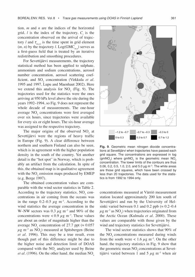
For Sevettijärvi measurements, the trajectory statistical method has been applied to sulphate, ammonium and sodium concentrations, aerosol number concentration, aerosol scattering coef-fi cient, and SO

2 concentration (Virkkula et al.

1995 and 1997, Lupu and Maenhaut 2002). Here we extend this analysis for NO

2 (Fig. 9). The

trajectories used for the statistics were the ones arriving at 950 hPa level above the site during the years 1992–1994, so Fig. 9 does not represent the whole decade of measurements. The one-hour average NO

2 concentrations were fi rst averaged

over six hours, since trajectories were available for every six or eight hours. The six-hour average was assigned to the respective trajectory.

The major origins of the observed NO2 at

Sevettijärvi were the regions of heavy traffi c in Europe (Fig. 9). A clear difference between northern and southern Finland can also be seen, which is in agreement with the higher population density in the south of the country. Yet another detail is the “hot spot” in Norway, which is prob-ably an artifact from the calculation. In spite of this, the obtained map is in qualitative agreement with the NO

2 emission maps produced by EMEP

(e.g. Berge 1997).The obtained concentration values are com-

parable with the wind sector statistics in Table 2. According to the trajectory statistics, NO

2 con-

centrations in air coming from the oceans was in the range 0.2–0.5 µg m–3. According to the wind statistics the average concentration in the W–NW sectors was 0.3 µg m–3 and 90% of the concentrations were < 0.9 µg m–3. These values are about an order of magnitude higher than the average NO

x concentration of 27.7 ppt (≈ 0.057

µg m–3 as NO2) measured at Spitsbergen (Beine

et al. 1996). This may be a true result, even though part of this difference might be due to the higher noise and detection limit of DOAS compared with the NO

x analyzer used by Beine

et al. (1996). On the other hand, the median NOx

concentrations measured at Värriö measurement station located approximately 200 km south of Sevettijärvi and run by the University of Hel-sinki varied between 0.1 and 0.2 ppb (≈ 0.2–0.4 µg m–3 as NO

2) when trajectories originated from

the Arctic Ocean (Kulmala et al. 2000). These values are comparable with those given by the wind and trajectory statistics for Sevettijärvi.

The wind sector statistics shows that 90% of the NO

2 concentrations measured during winds

from the south were < 1.6 µg m–3. On the other hand, the trajectory statistics in Fig. 9 show that the geometric mean NO

2 concentrations at Sevet-

tijärvi varied between 1 and 5 µg m–3 when air

Fig. 9. Geometric mean nitrogen dioxide concentra-tions at Sevettijärvi when trajectories have passed each grid square. The concentrations are expressed in log (gmNO2) where gmNO2 is the geometric mean NO2 concentration. The lower limits of the contours are thus 0.06, 0.2, 0.5, 1.0, 2.0, and 5.0 µg m–3. The white areas are those grid squares, which have been crossed by less than 20 trajectories. The data used for the statis-tics is from 1992 to 1994 only.

–1.2 to –0.7 –0.7 to –0.3 –0.3 to 0

0 to 0.3 0.3 to 0.7 0.7 to 1.2


comes from continental European sources south of Finland and Sweden. Kulmala et al. (2000) reported median NO

x concentrations of around 1

ppb (≈ 2 µg m–3 as NO2) in Värriö for air masses

originating from Western, Central and Eastern Europe. These values are again comparable with each other.

Although the highest NO2 concentrations

were observed during pollution episodes from Nikel, the trajectory statistics do not assign the highest values there. This discrepancy can prob-ably be explained by the area-averaging of the trajectory statistical procedure: the industrial area in Nikel is not very large and the statistics averages also the neighboring areas with low NO

x emissions into the same grid cell.

Conclusions

The DOAS instrument was used for a decade to measure the concentrations of gaseous SO

2, NO

2

and O3. The instrument worked quite reliably

during the whole time, even though there were some long discontinuities in the data which made a quantitative trend analysis diffi cult. Anyhow, our data show that the maximum hourly SO

2 con-

centrations decreased from around 500 µg m–3 during the fi rst two years of the monitoring to 200–300 µg m–3 in the mid 1990s. The annual average SO

2 concentrations decreased from

about 5 µg m–3 to 3–4 µg m–3 during the same period when taking into account the years for which the data coverage was above 85%. These values are lower but basically in agreement with measurements conducted by Norwegians. It has been observed that SO

2 emissions from Nikel,

and thereby concentrations measured at Svanvik, have remained more or less at the same level after a clear decrease from the 1980s to the early or mid 1990s. For NO

2 and O

3 concentrations no

clear trend was observed in this study.The sources of the three trace gases were

studied using wind measurements and in the case of NO

2 also using back trajectories. The trajec-

tory analysis is an extension to our earlier source analyses that have given a good picture on the transport of both gases and aerosols to Sevet-tijärvi. Since the pollutant sources are hundreds, even thousands, of kilometers away, the obtained

results are applicable to most of northernmost Fennoscandia. This can be seen, for example, when comparing NO

2 concentrations measured

in Sevettijärvi with NOx

concentrations meas-ured at a site 200 km south of Sevettijärvi.

References

Barrie L.A. 1986. Arctic air pollution: an overview of current knowledge. Atmos. Environ. 20: 643–663.

Barrie L.A., Olson M.P. & Oikawa K.K. 1989. The fl ux of anthropogenic sulphur into the Arctic from mid-latitudes in 1979/80. Atmos. Environ. 23: 2505–2512.

Beine H.J., Engardt M., Jaffe D.A., Hov Ø, Holmén K. & Stordal F. 1996. Measurements of NO

x and aerosol

particles at the Ny Ålesund Zeppelin mountain station on Svalbard: infl uence of regional and local pollution sources. Atmos. Environ. 30: 1067–1079.

Berge E. 1997. Transboundary air pollution in Europe, Part 1: Emissions, dispersion and trends of acidifying and eutrophying agents, EMEP MSC-W Status Report 1997, The Norwegian Meteorological Institute, Research Report no. 48, 108 pp.

Berresheim H., Wine P.H. & Davis D.D. 1995. Sulfur in the atmosphere. In: Singh H.B. (ed.), Composition, chemis-try, and climate of the atmosphere, Van Nostrand Rein-hold, New York, pp. 251–307.

Edner H., Ragnarson P., Spännare S. & Svanberg S. 1993. Differential optical absorption spectroscopy (DOAS) system for urban atmospheric pollution monitoring. Appl. Opt. 32: 327–333.

Feichter J., Kjellström E., Rodhe H., Dentener F., Lelieveld J. & Roelofs G.-J. 1996. Simulation of the tropospheric sulfur cycle in a global climate model. Atmos. Environ. 30: 1693–1707.

Finlayson-Pitts B.J. & Pitts J.N. 1986. Atmospheric chemis-try: fundamentals and experimental techniques. Wiley, New York, 1098 pp.

Fridlind A.M. Jacobson M.Z., Kerminen V.-M., Hillamo R.E., Ricard V. & Jaffrezo J.-L. 2000. Analysis of gas-aerosol partitioning in the Arctic: Comparison of size-resolved equilibrium model results with fi eld data. J. Geophys. Res. 105: 19891–19903.

Hagen L.O., Sivertsen B. & Arnesen K. 2002. Grenseom-rådene i Norge og Russland. Luft- og nedbørkvalitet, April 2001–Mars 2002, NILU Rep. OR 49/2002, Norwe-gian Institute of Air Research.

Kerminen V.-M., Aurela M., Hillamo R.E. & Virkkula A. 1997. Formation of particulate MSA — deductions from size distribution measurements in the Finnish Arctic. Tellus 49B: 159–171.

Kerminen V.-M., Teinilä K., Hillamo R. & Mäkelä T. 1999. Size-segregated chemistry of particulate dicarboxylic acids in the Arctic atmosphere. Atmos. Environ. 33: 2089–2100.

Kulmala M., Rannik Ü., Pirjola L., Dal Maso M., Karimäki J., Asmi A., Jäppinen A., Karhu V., Korhonen H., Mal-


vikko S.-P., Puustinen A., Raittila J., Romakkaniemi S., Suni T., Yli-Koivisto A., Paatero J., Hari P. & Vesala T. 2000. Characterisation of atmospheric trace gas and aerosol concentrations at forest sites in southern and northern Finland using back trajectories. Boreal Env. Res. 5: 315–336.

Laurila T. 1999. Observational study of transport and pho-tochemical formation of ozone over northern Europe. J. Geophys. Res. 104: 26235–26243.

Lohmann U., von Salzen K., McFarlane N., Leighton H.G. & Feichter J. 1999. Tropospheric sulfur cycle in the Canadian general circulation model, J. Geophys. Res. 104: 26833–26858.

Lupu A. & Maenhaut W. 2002. Application and comparison of two statistical trajectory techniques for identifi cation of source regions of atmospheric aerosol species. Atmos. Environ. 36: 5607–5618.

Maenhaut W., Jaffrezo J.-L., Hillamo R., Mäkelä T. & Ker-minen V.-M. 1999a. Size-fractionated aerosol composi-tion during an intensive 1997 summer fi eld campaign in northern Finland. Nucl. Instr. Meth. Phys. Res. B 150: 345–349.

Maenhaut W., Rajta I., Francois F., Aurela M., Hillamo R. & Virkkula A. 1999b. Long-term atmospheric aerosol study in the Finnish Arctic: Chemical composition, source types and source regions. J. Aerosol Sci. 30: S87–S88.

Raatz W. 1989. An anticyclonic point of view on low-level tropospheric long-range transport. Atmos. Environ. 23: 2501–2504.

Ricard V., Jaffrezo J.-L., Kerminen V.-M., Hillamo R.E., Teinilä K. & Maenhaut W. 2002. Size distributions and modal parameters of aerosol constituents in Northern Finland during the European Arctic Aerosol Study. J. Geophys. Res. 107 (D14), doi:10.1029/2001JD001130.

Ricard V., Jaffrezo J.-L., Kerminen V.-M., Hillamo R.E., Sillanpää M., Ruellan S., Liousse C. & Cachier H. 2002. Two years of continuous aerosol measurements in northern Finland. J. Geophys. Res. 107(D11), doi:10.1029/2001JD000952.

Seinfeld J. & Pandis S. 1998. Atmospheric chemistry and physics: from air pollution to climate change. Wiley, New York, 1326 pp.

Scheel H.E., Areskoug H., Geiß H., Gomiscek B., Granby K., Haszpra L., Klasinc L., Kley D., Laurila T., Lindskog

A., Roemer M., Schmitt R., Simmonds P., Solberg S. & Toupance G. 1997. On the spatial distribution and sea-sonal variation of lower-troposphere ozone over Europe. J. Atmos. Chem. 28: 11–28.

Simmonds P.G., Seuring S., Nickless G. & Derwent R.G. 1997. Segregation and interpretation of ozone and carbon monoxide measurements by air mass origin at the TOR station Mace Head, Ireland from 1987 to 1995. J. Atmos. Chem. 28: 45–59.

Stohl A. 1996. Trajectory statistics — a new method to estab-lish source-receptor relationships of air pollutants and its application to the transport of particulate sulfate in Europe. Atmos. Environ. 30: 579–587.

Stohl A. & Wotawa G. 1995. A method for computing single trajectories representing boundary layer transport. Atmos. Environ. 29: 3235–3239.

Tikkanen E. & Niemelä I. (eds.) 1995. Kola peninsula pol-lutants and forest ecosystems in Lapland. Final report of the Lapland Forest Damage Project. Finlandʼs Min-istry of Agriculture and Forestry and The Finnish Forest Research Institute, Gummerus, Jyväskylä, 82 pp.

Tuovinen J.-P., Laurila T., Lättilä H., Ryaboshapko A., Brukhanov P. & Korolev S. 1993. Impact of the sul-phur dioxide sources in the Kola Peninsula on air quality in northernmost Europe. Atmos. Environ. 27A: 1379–1395.

Virkkula A. 1997. Performance of a differential optical absorption spectrometer for surface O

3 measurements in

the Finnish Arctic. Atmos. Environ. 31: 545–555.Virkkula A., Hillamo R.E., Kerminen V.-M. & Stohl A. 1997.

The infl uence of Kola Peninsula, continental European and marine sources on the number concentrations and scattering coeffi cients of the atmospheric aerosol in Finnish Lapland. Boreal Env. Res. 2: 317–336.

Virkkula A., Mäkinen M., Hillamo R.E. & Stohl A. 1995. Atmospheric aerosol in the Finnish Arctic: Particle number concentrations, chemical characteristics, and source analysis. Water, Air, Soil Pollut. 85: 1997–2002.

Virkkula A., Aurela M., Hillamo R., Mäkelä T., Kerminen V.-M., Maenhaut W., Francois F. & Cafmayer J. 1999. Chemical composition of atmospheric aerosol in the European sub-Arctic: Contribution of the Kola Penin-sula smelter areas, Central Europe and the Arctic Ocean. J. Geophys. Res. 104: 23681–23696.

Received 31 January 2003, accepted 23 June 2003

a decade of trace gas measurements using doas in finnish lapland

Documents