a critical software review- how is hot … prediction and simulation of hot water in building design...

A CRITICAL SOFTWARE REVIEW- HOW IS HOT WATER MODELLED INCURRENT BUILDING SIMULATION?

Dashamir Marini1, Richard Buswell1 and Christina J. Hopfe1,1Building Energy Research Group, Loughborough University, UK

ABSTRACTIn a changing climate and with ever increasing energystandards that lead to low and zero energy buildings,the provision of hot water in buildings will becomemore significant in relation to the overall energy con-sumption. Higher demand on the provision of hot wa-ter consumption has been documented and will occuraround activities such as laundry, dishwashing, foodpreparation, bathing and cleaning activities. The accu-rate prediction and simulation of hot water in buildingdesign is therefore crucial and we need to rethink howwe estimate the amount of hot water in our buildings.This paper will investigate how hot water demand andprovision in homes is simulated via a number of dif-ferent tools. The input and output differences with re-spect to hot water are compared to measured data of abuilding in the UK.

INTRODUCTIONThe need for reducing energy consumption and green-house gas (GHG) emissions is a key challenge. TheUK Government has committed itself to reduce GHGby 80% in 2050 relative to the 1990 levels with the ob-jective towards zero emission from the domestic sectorDECC (2009). Based on this, building energy per-formance regulations and standards have been peri-odically updated introducing new performance valuescharacterized by a very high level of thermal insula-tion, with the aim to design ”zero energy” buildingsEPBD (2010). As a consequence, buildings becomemore energy efficient and airtight, therefore the pro-portion of energy demand for space heating to energydemand for hot water production is decreasing (note:space heating is not considered in this paper). It isestimated that hot water production accounts for 26%of the total energy consumption in residential homesDECC (2012). Therefore, the accuracy of hot waterdemand estimation is an important factor in order tobetter design and plan our domestic heating systemsand to predict more precisely the overall energy con-sumption. However, the methodologies (for estimat-ing hot water) that are implemented in regulations andstandards are often based on simplified methods andassumption.The design and provision of domestic hot water andenergy consumption is a challenging task as it de-pends on several unpredicted factors such as occu-pancy behaviour, appliances efficiency, mains supplyline pressure, supply water temperatures, heat genera-tion equipment, distribution system and other parame-ters that may vary from one household to another. The

building regulations are in a constant flux and the needfor better prediction of hot water demand is an impor-tant issue. In some cases monitored data has been usedto create hot water demand profiles, however the levelof detail of these models is not clear. From a literaturereview conducted in this paper it was found that sim-ulated results often do not match well with monitoreddata. In most cases, the main factors that contributeto this discrepancy between simulated and measuredresults are not investigated.The term ’hot water’ in this paper refers to the hot wa-ter used/produced to a certain temperature that satis-fies peoples comfort and hygiene requirements. Thedomestic hot water is mainly produced from the boilerand distributed via different devices such as taps, sinksshower/bath. There are however appliances such asdishwashing and washing machines which require hotwater generation to accomplish the cleaning activities.These appliances although not connected to the boiler,are built to produce and use hot water. As a conse-quence they are seen as appliances that consume hotwater and energy and therefore are considered in themeasurements and models of this paper.In this paper a literature review is carried out in or-der to investigate hot water demand assessment basedon current regulations. Further, a case study is pre-sented and a comparative analysis is carried out in or-der to compare the output of five different tools for atypical residential building. For reasons of sensitivityand fairness, we have chosen not to name the softwaretools used. We do not feel that this distracts from thescientific merits of the paper. The results include thevolume of hot water, energy consumption, heat losses,equipment efficiency and water flow temperatures. Ina critical review, we point out possible factors that in-fluence the discrepancy between the measured and thesimulated results. The overall aim of this paper is toaddress issues that can improve methods for modelsestimation and reduce software’s simulation shortcom-ings.

METHODSThe research was carried out in two parts: a literaturereview, important to understand the context of currentregulations and standards and a software review thatinvestigated the features and capabilities of simulationsoftwares with respect to hot water demand.

Part 1: Literature ReviewThe European standards such as CEN and CENELECdefine three tapping cycles and patterns ranging from

Proceedings of BS2015: 14th Conference of International Building Performance Simulation Association, Hyderabad, India, Dec. 7-9, 2015.

- 2417 -

11 to 30 draw-offs per day. This is whilst the to-tal volume of use ranges from 36 to 420 litres perday of hot water demand for a single household (Eu-ropean Commisison, 2002). The Code for Sustain-able Homes (CSH) suggests that the assessment cri-teria for total (hot+cold) water consumption in newdwellings should range from 80 to 120 litre per per-son a day (DCLG, 2010). Burzynsky et al. (2010) re-viewed methodologies used to estimate hot water de-mand and noted that there is only a limited numberof methods. They considered the BREDEM model asthe most advanced one. The hot water consumptionaccording to the BS EN-8558 (2011) standard shouldbe estimated between 35 to 45 litres per person perday. This is whilst BSRIA rules of thumb propose adaily hot water consumption between 80 to 120 litresper person per day (Hawkins, 2011) . The CEN Man-date 324 (2002) specifies a series of hot water run-offprofiles over 24 hours period associated with the vol-ume and energy consumed for each draw-off. Accord-ing to this standard, the average energy consumptionis about 4.3 kWh/day whilst the average volume ofhot water use is about 116 litres/day. Jordan and Va-jen (2005) developed a tool to generate DHW profilesbased on IEA-SHC Task 26 and used statistical meth-ods to distribute the draw-offs patterns. Garbai et al.(2014) used a methodology based on probability the-ory to predict hot water demand for a number of apart-ments considering quantity and intensity as stochas-tic variables. They found out that the quantity of hotwater consumed in a peak period of discretionary du-ration resembles a normal distribution. Makki et al.(2013) used a linear multiple regression analysis tocreate a shower end use forecasting model and re-vealed that variables, such as household makeup, oc-cupation status and shower-head efficiency are deter-minant variables for hot water use. A transient simu-lation program was developed by Rodriguez-Hidalgoet al. (2012) to obtain the dimensioning criteria of adomestic hot water solar plant and the size of the stor-age tank for a multi storey apartment building. Ay-ompe et al. (2011) validated a solar water heating sys-tems modelled with TRNSYS against measured dataand found out that mean absolute errors ranged from7% to 18 %. Kenway et al. (2012) developed a detailedmathematical flow analysis model to estimate house-hold water use. They found out that the model devia-tion error was within 20% of the monitored data. Ac-cording to a study carried out by Bennett et al. (2013)the application of Artificial Neural Networks (ANN)based modelling is a feasible method of producingmoderate accurate residential water demand end useforecasting models. Moreau (2011) simulated a stor-age water heating system with TRNSYS and validatedsimulated results against measured data. He found outthat the model was able to accurately predict the elec-tricity demand and the hot water temperature leavingthe tank. Lutz (2010) evaluated the hot water temper-

atures and flow rates as calculated by the combinedHWSim and TANK simulation models. His results re-vealed negligible differences.Cahill et al. (2013) modelled and simulated hot waterdemand for a dwelling using end-water-use parame-ter probability distributions generated by Monte Carlosimulations. They found out that the results were com-parable to their measurements. Lutz et al. (2013) usedMODELLICA to model storage and instantaneous wa-ter heaters systems with the aim to improve models inexisting libraries. The authors pointed out that the tooland existing models still needed to be improved, em-phasizing system control and distribution system mod-elling. Ries et al. (2013) used the BEopt optimiza-tion software to simulate and predict the performanceof a tankless water heater under retrofitting options.The authors pointed out that the demand patterns ofhot water demand influence the feasibility of the en-ergy reduction estimated from retrofitting. Wang et al.(2007) used ESP-r to model a gas-fired water storagetanks system and found that the model could predictthe mean tank temperature well. However, dependenton the water drawing schedule the energy consump-tion was underestimated by ca. 8-15%. In a studyby Clarke et al. (2009), they created hot water energymodels and indicated that the optimization of hot watersystem design (such as boiler location, controls, cylin-der sizing, distribution pipes and insulation) could pro-vide significant reduction of hot water and energy con-sumption.

Part 2: Modelling ApproachThe aim of the modelling approach is to estimatethe hot water volume used and the energy consump-tion for hot water production in the home. This in-cludes hot water from the taps, showering (boilersystem), dishwashing, and washing machines (appli-ances). The estimation of energy consumption (gasfor boiler and power for appliances) has been directlymeasured, whilst the hot water has been measuredonly for the boiler system. Meanwhile for the ap-pliances an approximate estimation was made whichis based on the measured power consumption techni-cal data sheet information. For each created model,the input parameters such as draw-off profiles, boilercapacity/efficiency, supply temperatures are based onthe default values for each of the chosen tools. Thephysical input parameters of the DHW system suchas, distribution pipe length and diameter are based onthe real measured values of the case study building,such as the total building floor area. In terms of thedishwasher (Zanussi 12001WA model as for this casestudy), the technical manual defines five different run-ning cycles, each of which has a certain duration, en-ergy consumption, temperature set point and hot wa-ter volume. Based on the cycles duration (estimatedfrom the measured power), and information from thetechnical manuals, the hot water volume was estimated


- 2418 -

Figure 1: Internal layout of the building

Table 1: Case study parameters of the monitored domestichot water system that serve as input for the simulation mod-els.

Parameter Value UnitBoiler capacity (Max/Min) 29/10 kWBoiler efficiency 87.1 -Flow rates (Max/Min) 11/2 l/minDistribution pipe inside diameter 0.0175 mDistribution branches total length 15 mTotal Draw-off points 7 qty

(short cycles, as defined in the technical manual wereconsidered as pre-wash and cold water is assumed tobe used). The same approach was applied for thewashing machine (Indesit WG1034 model).

Case studyA typical residential building located in Loughbor-ough (UK) was considered for modelling and gather-ing the measured data. The building is a two storeybuilding, constructed in the mid 1970’s with four bed-rooms covering 140m2(Figure2). It has a filled cavitywall insulation and is double glazed throughout. Thebuilding is part of the LEEDR project which moni-tored the hot water and energy consumption in twentyhomes at high resolution timestep. The heat genera-tion and draw-off characteristics of hot water use wereestimated for some homes and it was found that con-siderable (about eighteen percent) of total energy isconsumed solely by the hot water production (Buswellet al., 2013).Figure 1 shows the layout of the building and its do-mestic hot water system (red lines). The boiler is lo-cated on the first floor serving hot water bathroomtaps on the same floor and kitchen and toilet taps onground floor. Heating and hot water is provided in-stantaneously by a condensing combi-boiler (VokeraCompact 29H), serving radiators of varying size andstyle throughout the house. All radiators have manu-ally controlled thermostatic radiator valves. The houseis occupied by two adults and two children aged 11and 8. Table 1 presents the main parameters of themonitored system. From the boiler technical data-sheets, the capacity refers only to the hot water pro-duction (not including heating) as based on the waterflow limits and on an average temperature rise (∆T)35oC . The rating efficiency is based on the techni-cal manual and the average seasonal efficiency of thedomestic boiler. The distribution of the hot water sys-

Figure 2: Case study building (left) and simulated (right).

tem is constructed from uninsulated copper pipe andseven draw-off points for different end use categories(such as one shower, five taps and one bath tube) areconnected in total. Hot water is also used by other ap-pliances in the home such as dishwasher and washingmachine. However, these devices are not connected tothe domestic hot water system. In terms of measure-ments for the case study, the hot water mass flow rate,mains (inlet) and supply (outlet) water temperaturesin/out from the boiler are measured at a sample rate ofevery second, so that water volume, supplied thermalheat, mains supply and temperature rise (difference)for hot water can be estimated. The gas consumptionfrom the boiler was measured at a secondly time step,while the power consumption of devices such as dish-washer and washing machines (and all other electri-cal devices in the home) were measured at minutelytime step. Devices used and measured methods imple-mented in the case study are described in Marini et al.(2015).

OVERVIEW SOFTWARE TOOLSWe compared five different simulation tools with re-spect to the hot water demand and energy consumptionbased on different regulations and standards. Table 2summarizes the results including capabilities and un-derlying methods of the tools with respect to hot watermodelling as well as regulation compliances. In thefollowing a brief overview of the simulation tools ispresented.Tool A is a free dynamic simulation software with itscalculations based on BLAST and DOE-2 methods.The tool has been tested against the IEA BESTESTbuilding load and HVAC tests. The simulation mod-ules are integrated with a heat balance-based zone sim-ulation, and input/output data structures are tailored tofacilitate third party interface development. The ac-curacy and detailed simulation capabilities are consid-ered as tool strengths. Figure 3 shows a scheme ofdomestic hot water generated by Tool A.Tool B is a commercial dynamic simulation too. Itscalculation is based on: UK National Calculationmethodology (NCM), Part L, ASHRAE 55/ 90.1/62.1calculation procedures. The tool has been vali-dated and tested against several standards includingASHRAE 140/ BESTEST / CIBSE TM33 / EN13791.The tool can import files in different formats includ-


- 2419 -

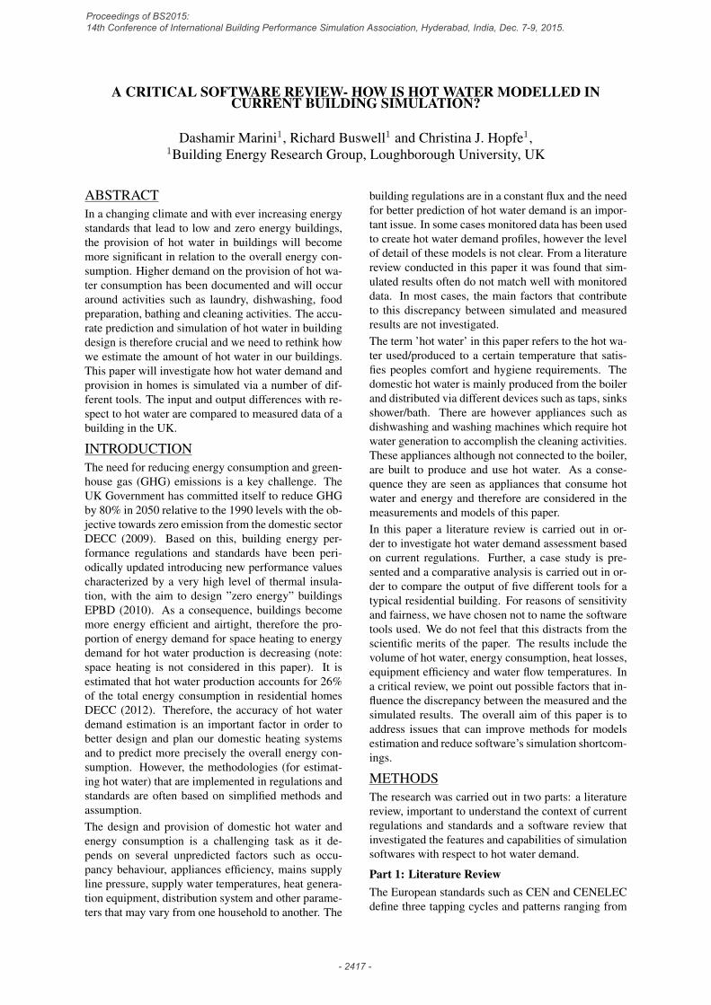
ing gbXML, IFC, DXF files. The data input is man-aged through graphical interfaces and supported bydatabases and component libraries.Tool C is a commercial tool that calculates the build-ing energy demand in static regime in compliance withinternational standards (ISO 13790). It has been val-idated using dynamic simulation tools and measureddata. The energy design and thermal comfort for highperformance buildings, especially passive houses areconsidered as strengths of the tool whilst multizonalmodelling for buildings and high need for control isnot possible.Tool D is a commercial static simulation tool where aspreadsheet is used to carry out the modelling and cal-culations. The procedure is consistent with the BS ENISO 13790 standard. The tool is adopted by UK Gov-ernment as the methodology and provides a frameworkfor the calculation of energy use in dwellings.Tool E is a free static simulation tool. Its calculationsare based on the UK National Calculation Methodol-ogy (NCM) which was developed in compliance withPart L2A of the building regulation. The softwaremakes use of standard data sets for different activityareas and calls on databases of construction and build-ing service elements.The input parameters (summarized in tables 3 and 4)for the simulation models, are based on: standards andregulations (see table 3, e.g. hot water demand, roomtemperatures, operational schedule), softwares defaultvalues (e.g. boiler efficiency, inlet/outlet supply tem-peratures; taps frequency; clothes and dishwashingfrequency) and on the real case study or practitionervalues (e.g. floor area, occupancy, boiler capacity,peak flow rate, pipe length/diameter and thermal con-ductivity). For each model, the input parameters are amixture of these input categories.

Modelling setupThe simulation input parameters necessary from soft-ware’s to calculate hot water demand and energy con-sumption for domestic hot water production are pre-sented in Tables 3 and 4 . The domestic hot water pro-file represents the average water use and includes wa-ter used from all end-use categories such as showers,baths, sinks, dishwasher and washing machine. Thewater demand defined for Tool A based on a normal-ized hourly profile ”masks” the boiler nominal designcapacity as it does not specify the real peak flow rate.The peak flow rate is based on a normalized hourlyload with a peak load of 20.2 l/hr (0.0056 l/s) it bringsthe design capacity up to an unrealistic value (900 W)for an assumed temperature rise of 35 oC . As a conse-quence a maximum flow rate of 0.15 l/s or 9 l/min (i.eshower maximum flow) was assumed to estimate a re-alistic nominal capacity. Fractions of realistic designflow rate were calculated and inserted into the programin order to produce the normalized hot water demandprofile as defined by the standard. The supply water

Figure 3: Tool A screen-shot input (left) and domestic hotwater system diagram (right).

outlet temperature is considered on average 50oC (hotwater only) for all end use categories whilst the mainwater inlet supply temperature (Schedule-5) is calcu-lated as a function of outdoor air temperature utilizingthe calculation formula defined in the calculation man-ual of Tool A. Tool B estimates the hot water demandbased on Part L2010 where each zone of the buildinghas a different demand value (Design-1) and is a func-tion of occupancy design level and operation sched-ules. The design values represent hot water demandfor all end-use categories. The occupancy level variesbetween the zones (Design-3) and it varies throughoutthe day.The domestic hot water system as part of the heatingsystem is modelled in ApacheHVAC where standardboiler efficiency and performance curve parametersare selected from default values. The ApacheHVACsystem (different from Apache which is a fully autosized and ideally controlled system) allows detaileddynamic modelling of the system, equipment and con-trols to be fully integrated within the thermal simula-tion model at every time step. The supply tempera-tures from cold water mains and hot water outlet aredefined constant through the simulations. Tool B es-timates heat losses from storage tank and secondarycirculations (not applicable for our case study) but itdoes not estimate the heat losses from the distributionsystem. Tool C for residential buildings assumes a de-fault design value for hot water demand as defined inTable 3 and includes all end-use categories such as:taps, sink, shower and bath.The defined boiler efficiency and supply (inlet/outlet)water temperatures are considered constant a through-out the entire period. The geometrical parameters ofthe distribution system, frequency of taps and roomtemperatures are used from the tool to estimate heatloss from dead-legs. The dishwasher and washing ma-chine are considered as appliances that consume coldwater by the software and are treated in separation.Tool C considered an average energy consumption of1.1 kWh for the dishwasher and the washing machine


- 2420 -

Table 2: Summary and overview of five different software tools used to predict hot water consumption.

Features and Capabilities Simulation SoftwareTool A Tool B Tool C Tool D Tool E

Version 8.0.0 2014.6.5.0 8.5 9.92 5.2.dAvailability Free Commercial Commercial Commercial FreeUser Interface TextInput Tabular/Graphical Tabular Tabular TabularRegulation Compliance ASHRAE1 PartL/CIBSE2/ASHRAE ISO3 13790 EPBD4 PartL/EPBDCalculation Methodology BLAST5/DOE6 UK NCM 7 /ASHRAE ISO 13790 BREDEM 8 UKNCM/CEN9

Simulation Engine DOE ApacheSim Excel Excel ExcelSimulation Regime Dynamic Dynamic Static Static StaticSimulation Timestep Minutely Minutely Hourly Daily HourlyOutputs Interface CSV/Tabular. Tabular/Graphical Spreadsheet Spreadsheet SpreadsheetOutputs Timestep Minutely Minutely Monthly Monthly MonthlySystem Simulation (T/S)10 Yes/Yes Yes/Yes Yes/Yes Yes/Yes Yes/YesHeat Losses (D/S/C)11 Yes/Yes/No No/Yes/Yes Yes/Yes/Yes Yes/Yes/No Yes/Yes/Yes

1 American Society of Heating, Refrigerating, and Air-Conditioning Engineers;2 Chartered Institution of Building Services Engineers;3 International Organization for Standardization;4 Energy Performance Building Directive; 5 Building Loads Analysis and Systems thermo-

dynamics;6 US Department of Energy; 7 United Kingdom National Calculation Method 8 Building Research Establishment Domestic EnergyModel; 9 European Committee for Standardization; 10 T-Tank; S-Solar;; 11 D-Distribution; S-Storage; C-Secondary circulation

Table 3: Design input parameters for the five simulated models.Parameter Unit Tool A Tool B Tool C Tool D Tool E

Litres/hour Schedule-1Litres/Person/hour Design-1a

Hot Water Demand Litre/Person/Day 25Litre/Day 109bSchedule-2 c

Litre/day/m2 Design-2Floor Area m2 143 143 143 143 143Occupancy Person 4 Design-3d 4 2.9 Design-3

Boiler Capacity kW 22.4 22.4 autosize -e -Boiler Efficiency - 0.8 0.81 0.84 Schedule-3 0.81Peak Flow Rate m3/s 0.00015 - - - -

Boiler PLR Efficiency Curve - Cubic Cubic - - -Outlet Supply Temperature 0C 50 60 60 Schedule-4f 60Inlet Supply Temperature 0C Schedule-5 10 11.2 - 10

Pipe Length m 15 - 15 - -Pipe Inside Diameter m 0.018 - 0.018 - -

Pipe Outside Diameter m 0.020 - 0.020 - -Pipe Thermal Conductivity W/(mK) 384 - 384 - -

Room Temperature 0C Schedule-6 g - 20 - -Taps Frequency Times/Person/day - - 3 - -

ClotheWashing/DishWashing Frequency Times/Person/year - - 57/65 - -Building Zones

Dining Kitchen Longue Bedroom Bathroom Toilet Common/Circulation areasDesign-1 11.8 11.8 6.6 2.5 14.9 37.9 0/45Design-2 1.05 1.05 0.72 0.53 1.05 4.85 0/2.6Design-3 59 42 53.3 43.6 50.3 41 9.4/11.2

Schedule-Fractions h SchF-Din SchF-Kit SchF-Lon SchF-Bed SchF-Bath SchF-Toi SchF-Cira Design values according zones ; b Volume derived from occupancy and zones floor area; c Schedule fractions of monthly hot water use ;d Design occupancy level for each zone of building (m2/person); e (-) Parameter not input in softwares for DHW system calculations;f Temperature rise of hot water production ∆T (not outlet supply); g Design heating set-point temperatures (used to calculate heat losses)

h Schedules fractions (SchF-Din –SchF-Cir) of zones occupancy level used from Tool B and Tool E software

Table 4: Operation schedules for the five simulated models.Time of Day (hr)

1 2 3 4 5 6 7 8 9 10 11 12 13 14 15 16 17 18 19 20 21 22 23 24Schedule-1 1.5 0.8 0.2 0.2 1.1 5.1 18.9 20.2 19.2 17.1 15.4 12.3 10.6 9.6 8.4 9.6 10.8 14.7 17.4 16.4 14.9 12.1 10.6 5.8SchF-Din 0 0 0 0 0 0 0 0 0 0 0 0 0 0 0 0 0.5 0.5 1 1 1 1 0.65 0SchF-Kit 0 0 0 0 0 0 0 1 1 1 0 0 0 0 0 0 0 0 0.2 0.2 0.2 0.2 0.2 0SchF-Lon 0 0 0 0 0 0 0 0 0 0 0 0 0 0 0 0 0.5 0.5 1 1 1 1 0.65 0SchF-Bed 1 1 1 1 1 1 1 0.5 0.25 0 0 0 0 0 0 0 0 0 0 0 0 0 0.25 0.75SchF-Bath 0 0 0 0 0 0 0 1 1 1 0 0 0 0 0 0 0 0 0.2 0.2 0.2 0.2 0.2 0SchF-Toi 0 0.8 0 0 0 0 0.5 1 1 0.25 0 0 0 0 0 0 0 0 0.5 1 1 0.3 0 0SchF-Cir 0 0 0 0 0 0 0 0.5 0.5 0.25 0 0 0 0 0 0 0.2 0.75 1 0.5 0.4 0.2 0.2 0

Month of Year1 2 3 4 5 6 7 8 9 10 11 12

Schedule-2 1.10 1.06 1.02 0.98 0.94 0.90 0.90 0.94 0.98 1.02 1.06 1.10Schedule-3 0.84 0.84 0.84 0.84 0.84 0.75 0.75 0.75 0.75 0.84 0.84 0.84Schedule-4 41.2 41.4 40.1 37.6 36.4 33.9 30.4 33.4 33.5 36.3 39.4 39.9Schedule-5 6.0 5.1 7.8 8.8 12.4 15.6 18.6 17.7 14.5 11.3 8.3 6.4Schedule-6 20 20 20 20 25 25 25 25 25 20 20 20


- 2421 -

Figure 4: Estimated results comparing the measured data with the output of the five simulation tools; showing the results for (a)Volume [m3], (b) Energy Consumption [kWh/m2], (c) Energy Losses [kWh], (d) Efficiency [-], (e) Main Supply Temperature[0C], (f) Temperature Difference [0C].

for each time of use. This is converted into primary en-ergy consumption utilizing a conversion factor of 2.6as defined in the calculation spreadsheet. Tool D esti-mates hot water demand based on the number of peo-ple. This parameter is calculated as a function of thetotal building floor area. The model assumes a vari-ability of hot water demand over the months and thisvariation is considered in the calculations as utiliza-tion factors (Schedule-2). The efficiency of boilersand temperature rise (∆T) are considered differentlyfor each month and are presented in Schedule-3 andSchedule-4 respectively. The calculation equations forhot water demand are described in the Tool D manualBRE (2012) whilst the software assumes 15% of totalhead demand for hot water production for distributionheat loss.Tool E estimates the hot water demand based on theBuilding Research Establishment (BRE) method. Forresidential buildings the estimation method providesthe design values (Design-2) for each zone. The boiler

efficiency and supply inlet/outlet temperatures (as de-fined in the technical manual) are considered constantover the entire year BRE (2014). The heat loss fromthe distribution system are estimated by the softwareassuming 17% of total heat demand for hot water pro-duction. The energy consumption from condensingboiler, hot water flow rate and supply/outlet tempera-tures were measured at secondly timestep. The powerconsumed from dishwasher and washing machines aremeasured by using CT devices at minutely timestep.The volume of water consumed by these devices hasbeen estimated based on measured power consump-tion and assumed water temperature rise as based onthe technical manuals. An in-situ measurement cal-ibration process was carried out in order to validatethe accuracy of measuring for water flow and temper-ature sensors. For water flow sensor was found thatthe error gap was ±7% whilst for the temperature sen-sor the error was lower than ±1K. The measured gasconsumption was compared to meter readings and an


- 2422 -

error deviation of +5.5% was found. The measureddata were corrected with the coefficient factors foundfrom the calibration process.

RESULTS and DISCUSSIONFigure 4 presents the estimated results from measure-ments and the results from simulated models. The re-sults are presented on a monthly basis for each esti-mated variable.From the observed result it was found that Tool Aoverestimated the hot water demand and the energyconsumption considerably compared to the measureddata. The other tools (especially Tool D) under-estimated the hot water demand whilst the energyconsumption was overestimated considerably by ToolE. The mains cold water temperature was estimatedslightly lower for each model as compared to the mea-surements whilst the temperature difference was con-siderably higher in Tools B and E.The estimated efficiencies of the DHW system frommeasurements and simulation tools at monthly levelare presented in Figure 4 (d). On average, the esti-mated efficiency was found to be 71% from the mea-surements, 87% for Tool A; 83% for Tool B; 84% forTool C and 81% for Tool D and E. The considered effi-ciency from the models was found to be overestimatedby around 14% to 22% as compared to the estimatedefficiency from the measurements.Tool B and Tool D were found to have a more accurateestimation regarding the litres of hot water demand perperson per day but apparently the occupancy level asbased on the softwares calculation methodology wasunderestimated. From measurements it was found thatabout 0.058 kWh energy was consumed by the pro-duction of one litre hot water at an average temper-ature of 49oC whilst in the simulated model the con-sumption varied between 0.054 and 0.091 kWh/litre.This difference is mainly attributed to the overesti-mated assumed efficiency and the water flow temper-atures (mains supply/temperature difference) betweenmeasured and model considerations.Figure 5 on the top plot shows the normalised hourlyhot water demand profiles estimated from: measureddata (blue line), Tool A (red line) and Tool B (greenline). Tool A shows clearly a higher demand profilecompared to the measured profile, except for the latenight hours.Tool Bs hot water demand is directly depended on theoccupancy profile. It can be noted that from 10:00 to16:00 there is no consumption as the tool assumed thatthere are no people in the home during this time. Themeasured data showed an unexpected demand profilefor the late night hours (00:00 to 05:00). The hot wa-ter consumption during this period was attributed towashing machine and dishwasher appliances. Thesedevices were used mostly during the night time. Thisunexpected pattern for these appliances was believedto be caused by the energy price policy (lower rates

Figure 5: Hot water demand profiles measured vs. models(top plot) measured categories (bottom plot).

for night hours usage). The bottom plot shows thebreakdown of the normalized measured hot water de-mand profile: the blue line represents the total hot wa-ter use in the home from all end use devices and ap-pliances; the green line represents the demand profilefrom the hot water system only (boiler supply) and thered line shows the sum of hot water used from washingmachine and dishwasher usage. The normalized term(used here and across the paper) describes the averagehot water use for each specific hour of the day as de-rived from the arithmetic mean 365 days of the year,representing an average normalized hourly hot wateruse for each our of the day throughout the year.

CONCLUSIONSIn this study five simulation tools were used to model aDHW system and compared based on respective soft-ware regulation compliances and calculation method-ologies. The simulated results were compared againstreal measured data gathered from a case study. Thevariables included hot water volume, energy consump-tion/losses, system efficiency, cold water supply tem-perature from mains and temperature rise (difference)for hot water production. It was found that the toolsunderestimated the hot water demand by about -30%and overestimated up to 40% as compared to the mea-sured data.The considered efficiency from the models was foundto be overestimated by 14-22% as compared to theestimated efficiency from the measurements. Themeasured supply water temperature from mains sup-ply pipeline on average was about 1.4-2.7oC higherthan what was considered by the simulation models.Meanwhile the temperature difference was found tobe overestimated by 1.2 to 14oC compared to the de-sign temperatures considered by the simulation mod-els. The temperature difference is considered as a con-stant value in each month by some software tools and


- 2423 -

Table 5: Difference percentage between measured and simulated for unit of volume and energy

Estimated Variable Unit Measured Simulated Values Difference measured vs. simulated (%)Tool A Tool B Tool C Tool D Tool E Tool A Tool B Tool C Tool D Tool E

Volume l/day 154 253 119 134 109 150 -39.1 22.7 12.9 29.2 2.5l/person/day 38 63 37 33 37.5 47 -39.1 2.6 15.1 1.3 -19.1

Energy Consumption kWh/day 9.1 13.8 6.8 9.5 7.8 13.6 -34.3 22.7 12.9 29.2 2.5kWh/litre 0.058 0.054 0.056 0.071 0.072 0.091 7.4 3.5 -18.3 -19.4 -36.2

Energy Losses kWh/day - 1.3 - 1.0 2.3 2.3 - - -30 43.4 43.4kWh/litre - 0.005 - 0.071 0.072 0.091 - - 29.5 30 45.1

therefore leads to an overestimation of the energy con-sumption.It can be concluded that: (a) The accuracy of hot wa-ter (i.e. daily consumption) is not explicitly dependenton the simulation tool and whether it is dynamic orsteady state. It rather depends on the considered de-sign values estimation procedure. For example, it wasfound that tool A (which is based on the US standard)significantly overestimated the hot water consumptioncompared to measurements and tools where the es-timation is based on the UK standard; (b) Dynamictools estimated the supply and temperature differencesmore accurately (i.e. monthly estimation opposed to ayearly estimation of the steady state tools); and (c) Dy-namic tools estimated the energy consumption and en-ergy losses per unit of hot water use more accurately.In summary, dynamic simulation tools can predict theresults more accurately (with input and output parame-ters at an hourly or less time step), however the scale ofthe accuracy is dependent on the respective standards.The fact that some of the results suggest an increasedefficiency and at the same time more energy consump-tion (Table 5), is likely caused by two main factors:the considered inlet/outlet design supply temperatures(consequently temperature difference) and the esti-mated energy losses. For example, although the steadystate tools C, D, E have a higher efficiency, the tem-perature differences are higher as well and constantthroughout the year, causing an overestimation of thepredicted energy consumption (Figure 4 and Table 5).

REFERENCESCEN Mandate 324 2002. Mandate to cen and cenelec for the elab-

oration and adoption of measurrement standards for householdappliances. Technical report, European Commission.

Ayompe, L., Duffy, A., McCormack, S., and Conlon, M. 2011. Vali-dated trnsys model for forced circulation solar water heating sys-tems with flat plate and heat pipe evacuated tube collectors. Ap-plied Thermal Engineering.

Bennett, C., Steward, R., and Beal, C. 2013. Ann-based residentialwater end-use demand forecasting model. Expert Systems withApplications. pg 1014-1023.

BRE 2012. Building Research Establishment. The Goverment’sstandard assessment procedure for energy ratings of dwellings.http://www.bre.co.uk/filelibrary/SAP/2012/SAP-2012-9-92.pdf.

BRE 2014. National Calculation Methodology. A technical manualfor SBEM . http://www.ncm.bre.co.uk/download.jsp .

BS EN-8558 2011. Guide to the design, installation, testing andmaintenance of services supplying water for domestic use withinbuildings and their curtilages-guidance to BS EN 806.

Burzynsky, R., Crane, M., and Yao, R. 2010. A review of domestichot water demand calculation methodologies and their suitabilityfor estimation of the demand for zero carbon houses. Proc ofTSBE EngD Confernce. Reading, United Kingdom.

Buswell, R., Marini, D., Webb, L., and Thomson, M. 2013. De-

termining heat use in residential buildings using high resolutiongas and domestic hot water monitoring. Proc of 13th BuildingSimulation.France.

Cahill, R., Lund, J., DeOreo, B., and Medellin-Azuara, J. 2013.Household water use and conservation models using monte carlotechniques. Hydrology and Earth System Sciences.

Clarke, A., Grant, N., and Thornton, J. 2009. Quantifying the energyand carbon effects of water savings. Technical report, Environ-ment Agency and Enrgy Saving Trust.

DCLG 2010. Code for Sustanable Homes. Technical guide, Depart-ment for Communities and Local Goverment.

DECC 2009. Carbon valuation in UK policy appraisal:A revised Approach, Department of Energy and Cli-mate Change. https : //www.decc.gov.uk/en /content/cms/statics/publications/ecuk.aspx.

DECC 2012. Household End Use Energy Consump-tion, Department of Energy and Climate Change.https://www.gov.uk/government/organisations/department-of-energy-climate-change.

EPBD 2010. Directive 2010/31/eu of the european parliament and ofthe council of 19 may 2010 on the energy performance of build-ings (recast). Official Journal of the European Union.

European Commisison 2002. Mandate to CEN and CENELEC forthe eleboration and adoption of measured standards for house-hold appliances: water-heaters, hot water storage appliances andwater heating systems.

Garbai, L., Jasper, A., and Magyar, Z. 2014. Probably theory de-scription of domestic hot water and heating demands. Energyand Buildings.

Hawkins 2011. Rules of thumb, guidelines for building services 5thedition (BSRIA Guide).

Jordan, U. and Vajen, K. 2005. Dhwcalc: Program to generate do-mestic hot water profiles with statictical means for user definedconditions. Proceedings of ISES Solar World Congres. US.

Kenway, S., Scheidegger, R., Larse, T., Lant, P., and Bader, H. 2012.Water-related energy in households: A model designed to under-stan the current state and simulation possible measures. Energyand Buildings.

Lutz, J. 2010. Evaluation of TANK water heater simulation modelas embedded in HWSim. Technical report, LBNL, .

Lutz, J., Grand, P., and Kloss, M. 2013. Simulation models forimproved water heating systems. Technical report, LBNL, .

Makki, A., Steward, R., Panuwatwanich, K., and Beal, C. 2013.Revealing the determinants of shower water end use consump-tion: enabling better targeted urban water conservation strategies.Journal of Cleaner Production. .

Marini, D., Buswell, R., and Hopfe, C. 2015. Estimating wasteheat from domestic hot water systems in UK dwellings. Proc ofBuilding Simulation 2015.

Moreau, A. 2011. Control strategy for domestic water heaters duringpeak periods and its impact on the demand for electricity. EnergyProcedia. pg 1074-1082.

Ries, R., Walters, R., and Dwiantoro, D. 2013. Analysis of the effec-tiveness of a simulation model for predicting the performance ofa tankless water heater retrofit. Proc of 13th Building Simulation.France.

Rodriguez-Hidalgo, M., Rodrigues-Aumente, P., Lecuona, A., andVentas, R. 2012. Domestic hot water consumption vs. solar ther-mal energy storage: the optimim size of the storage tank. AppliedEnergy. pg 897-906.

Wang, W., Beausoleil-Morrison, I., Thomas, M., and Ferguson, A.2007. Validation of a fully-mixed model for simulating gas-firedwater storage tanks. Proc of 10th Building Simulation. China.


- 2424 -

a critical software review- how is hot … prediction and simulation of hot water in building design...

Documents