a covariance model for markov statistics

www.elsevier.com/locate/anucene

Annals of Nuclear Energy 33 (2006) 1408–1416

annals of

NUCLEAR ENERGY

A covariance model for Markov statistics

Richard Sanchez

Commissariat a l’Energie Atomique, Direction de l’Energie Nucleaire, Service d’Etudes de Reacteurs et de Mathematiques Appliquees,

CEA de Saclay, France

Received 20 June 2006; accepted 14 August 2006Available online 28 November 2006

Abstract

We propose a model to compute the variances for the ensemble average material fluxes in line Markov statistics. The model is exact atthe limit of collisionless transport. The calculation of the material flux variances needs the determination of the covariances (in l and l 0)and we have developed a system of coupled equations and made the usual heuristic extension to the case with collisions. A simple numer-ical solution, based on the standard discrete ordinates approximation with the diamond discretization, is proposed in 1D slabs. Numer-ical applications are given for bimaterial homogeneous statistics. The results are encouraging but further research is needed in this area.This will involve a modification of the standard Levermore–Pomraning model.� 2006 Elsevier Ltd. All rights reserved.

1. Introduction

Transport in stochastic materials has applications inradiative transfer as well as reactor analysis. The relevantquantities of interest in this case are the so-called mate-

rial fluxes. These are the ensemble averaged fluxes forthe set of physical realizations that have a given materialin the same geometrical location. A system of exacttransport-like coupled equations for the material fluxeswas independently derived by Adams et al. (1989) andby Sanchez (1989), but these equations are not closed.Correlation terms appear that depend on new ensembleaveraged fluxes, called interface fluxes. These new fluxesare the averages over the realizations that have one mate-rial to the left of a geometrical location and a differentmaterial to the right of the location, along a given direc-tion of particle motion. In principle, a new set of trans-port-like equations could also be written for thetransition fluxes. An approximated second-order modelwas proposed by Pomraning (1991b) to tackle thisproblem but was later shown to be largely inaccurate(Zuchuat et al., 1994). This conclusion was corroboratedby an analysis of the mathematical structure of the sec-

0306-4549/$ - see front matter � 2006 Elsevier Ltd. All rights reserved.

doi:10.1016/j.anucene.2006.08.011

E-mail address: [email protected]

ond-order model which proved that the model proposedby Pomraning did not have the correct structure (San-chez, 1995).

This is the reason why, today, the model universallyused for the calculation of the material fluxes is based onan approximate closure of the material equations. Indeed,for line Markovian statistics the material equations havea natural closure in the absence of collisions. This is sobecause in these conditions the transition flux is equal tothe material flux for the upstream material. An approxi-mated model was earlier proposed by Levermore and Pom-raning. This Levermore–Pomraning model has come to beknown as the ‘standard model’. Pomraning (1991a)generalized the model to non Markovian line statistics bymodifying the average chord lengths so that an asymptoticflux solution was preserved. Although this generalization isnot exact, numerical results showed that it was relativelyaccurate.

However, regardless of the approximations involved, theknowledge of the material fluxes is not enough to sanctionits use in practical applications. Indeed, because the realiza-tion that one considers in a given problem is, of course,unknown, use of the material flux can result in a large errorif the statistical dispersion of the fluxes for the individualrealizations is large. Therefore, what is needed is a measure

mailto:[email protected]

R. Sanchez / Annals of Nuclear Energy 33 (2006) 1408–1416 1409

of the dispersion of the individual fluxes with respect totheir ensemble average. The quantity of interest is thematerial variance for the scalar flux. Pomraning (1996)developed a system of transport-like equations for the var-iance of the angular flux and closed this system with thefamiliar Markovian approximation. However, the materialvariance for the angular flux cannot be used to determinethe statistical dispersion around a given material scalarflux. As shown in this work, the quantity that is neededis the material covariance for the angular flux. Recently,Akcasu and Larsen (2003) used a drastic flux factorizationassumption to derive approximated equations for the mate-rial variances of the scalar fluxes in bimaterial mixtureswith Markovian statistics. Although these equationsaccount for isotropic scattering, there are exact only inthe absence of collisions.

In Section 2, we establish an exact system of transport-like equations for the material covariances. The analysis issimple and follows the general approach used earlier towrite the material flux equations. As expected, this systemof equations is not close because of correlation terms thatnow depend on interface covariances. Determination of asecond-order transport-like equation for these interfacecovariances run, alas, into the same difficulties alreadymet for the interface fluxes. We have considered line Mar-kov statistics and found that the material covariance equa-tions naturally close in purely absorbing materials.Following the dominant tradition in this area of research,we have opted for establishing a system of approximateequations by assuming that the closure is valid in the caseof collisions. Our final equations are written in terms of acovariance tensor from which one can straightforwardlycalculate the desired variances for the scalar materialfluxes.

In Section 3, we present numerical results for severalproblems from the set of benchmark problems proposedby Pomraning (1991a,b). The results are promising butnot conclusive. For optically thick slabs the calculationsmay give negative covariances or simply do not converge.This problem is related to the fact that the covarianceequations include a double approximation in the case withcollisions. The first comes from the replacement of theinterface covariances by the material ones, and the secondbecause the sources in these equations depend on the mate-rial fluxes, which are only approximate in the presence ofcollisions. These two approximations are a result of theMarkovian closure. Conclusion and further discussionare given in Section 4.

We have used a pedestrian discrete-ordinates diamond-differencing scheme to solve the equations for the covari-ance tensor. An interesting aspect, however, appearsbecause the covariance tensor depends on two cosines,Ta(x,l,l 0), a fact that requires special care in the numericalsolution. The details of the numerical discretization havebeen relegated to the Appendix.

This work is a revised version of a paper presented in arecent international topical meeting (Sanchez, 2005).

2. The Levermore–Pomraning model

For simplicity we consider slab geometry with transla-tionally invariant (homogeneous) bimaterial statisticsalong the line. The Levermore–Pomraning (LP) model(Adams et al., 1989; Sanchez, 1989; Pomraning, 1991a) isgiven by the equations

ðlox þ raÞwa ¼ H awa þ Sa þjljkaðwb � waÞ;

wað0; lÞ ¼ wa;inð0Þ; l > 0;

waðL; lÞ ¼ wa;inðLÞ; l < 0;

ð1Þ

where we have considered a slab with incoming flux onboth sides, ka is the average chord length for material aand we have denoted by a (b) the two deterministicmaterials.

In this equation H stands for the collision operator and

waðx; lÞ ¼R

XaðxÞ pðxÞdxwxðx; lÞpa

¼ MaðxÞ � wMaðxÞ � 1

is the ensemble average material flux at position x. Theaveraging is done on the subset Xa(x) = {x 2 X,x(x) = a} of realizations that have material a at positionx and wx(x,l) is the deterministic flux corresponding torealization x. Here X represents the statistical set of allphysical realizations. Notice also that pa(x) is constantfor homogeneous statistics.

For Markovian line statistics and collisionless transportequation (1) is exact (the Markovian closure). Benchmarkcalculations with collisions (Pomraning, 1991a; Zuchuatet al., 1994) have demonstrated that the LP model is robustand, because of its simplicity, this model has become to beaccepted as the ‘standard’ model. In principle, Eq. (1) canbe solved to compute an approximation (in the presence ofcollisions) of the material flux wa. However, a measure onthe dispersion of the wx(x,l) around the ensemble averagewa(x,l) is required if the result is to be of any practical use.

Pomraning (1996) considered a Markovian mixture oftwo immiscible purely absorbing materials and appliedthe master equation formalism to derive an exact descrip-tion for the ensemble average of any power of the angularflux

ðwnÞaðx; lÞ ¼MaðxÞ � wn

MaðxÞ � 1;

where Ma(x) is the averaging operator implicitly defined inEq. (1). But the quantity that is required is the variance ofthe scalar flux /xðxÞ ¼ 1

2

R 1

�1dlwxðx; lÞ,

r2aðxÞ ¼

MaðxÞ � ½ð/� /aÞ2�

pa

;

or, equivalently, the ensemble average of the square of thematerial flux

ð/2ÞaðxÞ ¼MaðxÞ � /2

pa

1410 R. Sanchez / Annals of Nuclear Energy 33 (2006) 1408–1416

from which the variance can be recovered: r2aðxÞ ¼

ð/2ÞaðxÞ � /2aðxÞ.

Recently, Akcasu and Larsen (2003) have proposed anapproximate equation for (/2)a(x) for bimaterial mixtureswith Markovian statistics. The equation was derived underthe rather drastic assumption that the angular and the sca-lar flux have the same spatial dependence, i.e., wx(x,l) =gx(l)/x(x) and, although it accounts for isotropic scatter-ing, it is exact only in the absence of collisions. However,the detailed expression

ð/2ÞaðxÞ ¼MaðxÞ � /2

pa

¼ 1

pa

ZXaðxÞ

pðxÞdx1

2

Zwx

ðx; lÞ" #2

¼ 1

2

Z 1

�1

dl1

2

Z 1

�1

dl0ðww0Þa;

where the prime denotes the argument l 0, w0x ¼ wxðx; l0Þ,shows that, when no approximation is introduced, whatit is really needed is the calculation of the covariance ofthe angular flux

ðwwÞaðx; l; l0Þ ¼MaðxÞ � ww0

pa

¼R

XaðxÞ pðxÞdxwxðx; lÞwxðx; l0Þpa

:

However, a more expedient way to obtain the scalar fluxvariance is to compute the covariance tensor

T aðx; l; l0Þ ¼ ðww0Þa � waw0a ð2Þ

from which one can directly obtain the variance for thematerial flux /a as

r2aðxÞ ¼

1

2

Z 1

�1

dl1

2

Z 1

�1

dl0T aðx; l; l0Þ: ð3Þ

In the first part of this work we present what we believe is anew extension of the LP model to compute the covarianceof wx(x,l) relative to the subset of realizations Xa(x).

3. Transport equation for the covariance

First, we establish an equation for wxw0x ¼ wx ðx; lÞwxðx; l0Þ and then apply the integral operator Ma(x) to thisequation to derive an equation for the covariance. Con-sider the deterministic equation for realization x

ðlox þ rxÞwx ¼ Hxwx þ Sx;

wxð0;lÞ ¼ wx;inð0Þ; l > 0;

wxðL; lÞ ¼ wx;inðLÞ; l < 0:

ð4Þ

Write a similar equation for wx(x,l 0), multiply the equa-tion for wx times l0w0x and the equation for w0x timeslwx and sum the resulting equations to obtain

½ll0ox þ ðlþ l0Þrx�wxw0x ¼ l0w0xqx þ lwxq0x;

ðwxwxÞð0; l; l0Þ ¼ wxð0; lÞwxð0; l0Þ;ðwxwxÞðL; l; l0Þ ¼ wxðL; lÞwxðL; l0Þ;

ð5Þ

where the corresponding form of the boundary valuesdepends on l and l 0.

In order to apply Ma(x) to this equation we need tointroduce the derivative of operator Ma(x) (Sanchez, 1989)

oxMaðxÞ ¼ MbaðxÞ �MabðxÞ: ð6ÞHere

MabðxÞ ¼ lime!0þ

1

e

ZXabðx;xþeÞ

pðxÞdx

We then apply (1/pa)Ma(x) to Eq. (5) and useMa(x) � oxf = ox[Ma(x) � f] � [ox Ma(x)] � f to obtain

½ll0ox þ ðlþ l0Þra�ðww0Þa ¼ ðl0w0qþ lwq0Þa

þ ll0

ka½ðww0Þba � ðww0Þab�;

ðwwÞað0; l; l0Þ ¼ wað0; lÞwað0; l0Þ except for l; l0 < 0;

ðwwÞaðL; l; l0Þ ¼ waðL; lÞwaðL; l0Þ; except for l; l0 > 0;

ð7Þwith q = Hw + S. Here (ww 0)ba and (ww 0)ab are interfacecovariances averaged on the set of realizations with changeper unit length, respectively, from material b into materiala and from material a into material b around x in the direc-tion of increasing x values

ðww0Þab ¼MabðxÞ � ðww0Þ

MabðxÞ � 1:

These new transition covariances are much alike to theequivalent transition fluxes wba and wab that are usedin the derivation of the standard equation (Sanchez,1989). For the source term in (7) we obtain the exactexpression

ðl0w0qþlwq0Þa ¼ l0½H 1aðww0Þaþw0aSa� þl½H 2

aðww0ÞaþwaS0a�;

where the scattering operator Hia acts on the ith flux

H 1aðwwÞaðx; l; l0Þ ¼

Z 1

�1

dl00rsaðl00 ! lÞðwwÞaðx; l00; l0Þ;

H 2aðwwÞaðx; l; l0Þ ¼

Z 1

�1

dl00rsaðl00 ! l0ÞðwwÞaðx; l; l00Þ:

ð8Þ

3.1. Equation for the covariance tensor

Next, to obtain an exact equation for the covariance ten-sor Ta in (2) we consider the exact equation for the covari-ance (7) and the exact equation for wa

ðlox þ raÞwa ¼ H awa þ Sa þlkaðwba � wabÞ;

wað0; lÞ ¼ wa;inð0Þ; l > 0;

waðL; lÞ ¼ wa;inðLÞ; l < 0:

Then, we write a similar equation for wa(x,l 0), multiply theequation for wa times l0w0a and the equation for w0a timeslwa and sum the resulting equations to obtain an equation


for the product waw0a. This equation is similar to Eq. (5) for

wxw0x

½ll0ox þ ðlþ l0Þra�waw0a ¼ l0w0aqa þ lwaq0a

þ ll0

ka½w0aðwba � wabÞ þ waðw0ba � w0abÞ�;

ðwawaÞð0; l; l0Þ ¼ wað0; lÞw0að0; l0Þ;ðwawaÞðL; l; l0Þ ¼ waðL; lÞw0aðL; l0Þ:

Finally, we subtract this equation from the equation forthe covariance, Eq. (7), and, after simplification ofcommon terms, we obtain the desired equation forTa(x,l,l 0)

½ll0ox þ ðlþ l0Þra�T a ¼ ðl0H 1a þ lH 2

aÞT a þ Ia;

T að0; l; l0Þ ¼ 0; except for l; l0 < 0;

T aðL; l; l0Þ ¼ 0; except for l; l0 > 0;

ð9Þ

where

Iaðx; l; l0Þ ¼ll0

kaf½ðww0Þba � w0awba � waw

0ba�

� ½ðww0Þab � w0awab � waw0ab�g: ð10Þ

Note that there are no volume of surface inhomogeneoussources, other than those in the coupling term Ia. The coef-ficients in Ia depend exclusively on the material fluxes. Eq.(9) is exact but introduces new interface moments. Further-more, Eq. (9) has a symmetrical solution, Ta(x,l,l 0) =Ta(x,l 0,l), and this proves that the covariance (ww 0)a isalso symmetrical.

3.2. Markovian closure

As it was done to derive the final form of (1) we considerEqs. (7) and (9) for Markovian statistics. These statisticsare characterized by the property that the probability forthe right trajectory at x, x+(x), depends only on the mate-rial at x(x�), where x� ¼ lime!0þðx� eÞ. For these statisticswe can write

fa ¼MaðxÞ � fMaðxÞ � 1

¼CaðxÞ

RX�ðxÞ p�ðx�Þdx�

RXþðxÞ pþðxþÞdxþfx

CaðxÞR

X�ðxÞ p�ðx�Þdx�R

XþðxÞ pþðxþÞdxþ;

fab ¼MabðxÞ � fMabðxÞ � 1

¼CabðxÞ

RX�ðxÞ p�ðx�Þdx�

RXþðxÞ pþðxþÞdxþfx

CabðxÞR

X�ðxÞ p�ðx�Þdx�R

XþðxÞ pþðxþÞdxþ:

ð11Þ

Here Ca(x) and Cab(x) (constant for homogeneous statis-tics) are two scaling factors that cancel in the numeratorand denominator.

We now investigate the case of collisionless transport(H = 0). For fx = wx(x,l) the angular flux wx dependsonly on the left (l > 0) or on the right (l < 0) trajectoryand the above equations give

wabðx; lÞ ¼waðx; lÞ; l > 0;

wbðx; lÞ; l < 0:

(

A property that was used to derive the Markovian closurefor collisionless transport and its heuristic extension, Eq.(1), to the case with collisions. Next, we use the Markovianproperty (11) to analyze the limit form of the covarianceequations for collisionless transport. In this case, and forfx = wx(x,l)wx(x,l 0), we obtain

ðwwÞabðx; l; l0Þ ¼

ðwwÞaðx; l; l0Þ; l; l0 > 0;

ðwwÞbðx; l; l0Þ; l; l0 < 0;

waðx; lÞwbðx; l0Þ; l > 0; l0 < 0;

wbðx; lÞwaðx; l0Þ; l < 0; l0 > 0:

8>>><>>>:

ð12ÞFinally, at the same limit, the correlation term (10) in theequation for the covariance tensor becomes

Iaðx; l; l0Þ ¼jljl0kaðT b � T a þ QaÞ; ll0 > 0;

0; ll0 < 0

(ð13Þ

with the source term

Qaðx; l; l0Þ ¼ ðwb � waÞðw0b � w0aÞ: ð14Þ

In the Markovian limit equation (9) gives an exact descrip-tion for the covariance. Note that in this limit the only con-tribution to Ta comes from the pairs of trajectories withl,l 0 < 0 and l,l 0 > 0. Also, at the atomic mix limit orfor identical mixed media (a = b) the tensor cancels outand the variance is zero, as it should be.

Finally, we make a heuristic extension to the case withcollisions by assuming that (13) holds also in the presenceof collisions.

In the Appendix we present a naive numerical methodfor the solution of the ‘standard’ model for the variances,as given by Eqs. (9) and (13).

4. Numerical results for Markovian statistics

All the calculations presented here were done with a S16

Gauss–Legendre quadrature formula and each result wascompared to the statistical mean obtained from S16 calcu-lations for 50,000 realizations. All calculations were donewith the diamond approximation and with a mesh size thatinsures positivity. For the uncollided cases the referenceresults are not shown because, as expected, they are identi-cal to those given by the LP model. In this section wepresent results for the material and ensemble average fluxesand their associated relative standard deviations

r ¼ 1

h/i

ffiffiffiffiffiffiffiffiffiffiffiffiffiffiffiffiffiffiffiffiffiffiffiffiffiffihð/� h/iÞ2i

q;

where Æ Æ æ indicates ensemble averaging.We consider the benchmark series of 27 problems pro-

posed by Pomraning (Levermore et al., 1988) for the anal-ysis of the propagation of an isotropic incident beam

Table 1The Pomraning’s benchmark series

Case R0 k0 R1 k1 Case c0 c1 L

1 10/99 99/100 100/11 11/100 a 0.0 1.0 0.12 10/99 99/10 100/11 11/10 b 1.0 0.0 13 2/101 101/20 200/101 101/20 c 0.9 0.9 10

Table 2Results for the transmission through the slab

Case Length Transmission rt # regions

1 0.1 8.9190 · 10�1 1.5915 · 10�1 2001 4.4316 · 10�1 7.1664 · 10�1 479

10 9.2703 · 10�4 6.2096 4785

3 0.1 8.4941 · 10�1 2.7630 · 10�2 2001 4.7420 · 10�1 4.4504 · 10�1 200

10 6.3940 · 10�2 2.7917 1043


through a binary Markovian mixture of two materials. Thedata for these problems is reproduced in Table 1.

Fig. 1 shows the results for the uncollided cases 1 and 3with L = 10 and with an incident isotropic angular flux onthe left side of the slab.

The results in Fig. 1 show that the predicted materialand ensemble average fluxes are not reliable for the bench-mark cases proposed by Pomraning. Indeed, the statisticaldispersion of the results increases very fast with the dis-

Case 1 Case 3 fl

uxes

and

rel

ativ

e st

anda

rd d

evia

tions

flux

es a

nd r

elat

ive

stan

dard

dev

iatio

ns

Fig. 1. Results for uncollided cases 1 and 3 with L = 10 and incoming isotropic flux on the left side of the slab.

S0 = 0 S1 = 1 S0 = 1 S1 = 1

flux

es a

nd r

elat

ive

stan

dard

dev

iatio

ns

flux

es a

nd r

elat

ive

stan

dard

dev

iatio

ns

Fig. 2. Results for uncollided case 3 with L = 1 and material sources. The fluxes have been rescaled to fit in the figure.


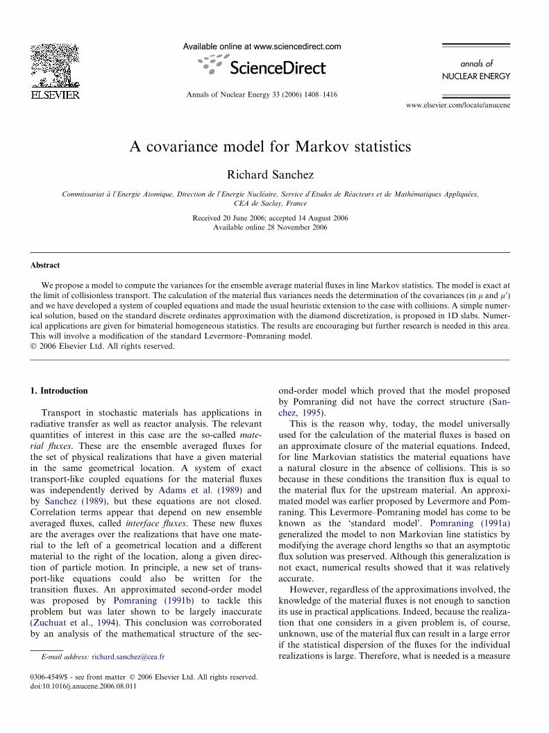
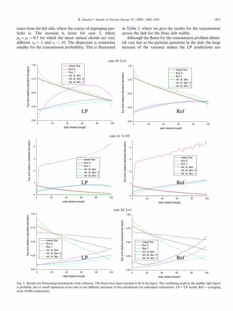
tance from the left side, where the source of impinging par-ticles is. The increase is faster for case 3, wherep0 = p1 = 0.5 for which the mean optical chords are verydifferent s0 = .1 and s1 = .10. The dispersion is somewhatsmaller for the transmission probability. This is illustrated

case 1b L

case 3

case 2c

LP

LP

LP

Fig. 3. Results for Pomraning benchmarks with collisions. The fluxes have beenis probably due to small numerical errors due to the different precision of thefrom 50,000 realizations.

in Table 2, where we give the results for the transmissionacross the slab for the three slab widths.

Although the fluxes for the transmission problem dimin-ish very fast as the particles penetrate in the slab, the largeincrease of the variance makes the LP predictions not

=1

d L=1

L=10

Ref

Ref

Ref

rescaled to fit in the figure. The oscillating result in the middle right figurecalculations for individual realizations. LP = LP model, Ref = averaging

LP Ref

Fig. 4. Fluxes and relative standard deviations for a 5 cm slab comprising a Markovian mixture of one material and vacuum. The material has c = 0.5 andthe system is fed with isotropic neutrons on the left side.


reliable for practical applications. For reactor applicationsthis conclusion applies to shielding problems with statisticsa la Pomraning. However, typical problems of interest inreactor analysis are dominated by volume sources thatdepend on the material that is present at a given location.One may expect that the presence of volume sources maydecrease the variance of the fluxes, especially when themean chord lengths are large enough to allow for a localequilibrium between sources and absorption. To check thisassumption we have run case 3 with L = 1 with materialsources. The results in Fig. 2 show that the variances aremuch more smaller. For the case with a constant sourcein material 1 the relative standard deviation is of the orderof 2.3 in the material without source, material 0, and of theorder of 0.08 for the material with the source. Whensources are present in both materials the relative standarddeviations are still smaller, of the order of 0.15 for material0 and of 0.2 for material 1. For a case with S0 = 0.01 andS1 = 1, not shown in the figure, the relative standard devi-ations are of the order of 1.44 and 0.08, respectively, formaterials 0 and 1.

It is to be expected that the standard deviations will besmaller with a case with collisions because collisions tendto smooth out the flux between the different materials.We have applied the LP variance model to the Pomraningbenchmarks. In Fig. 3, we give some of the results obtainedfor the Pomraning benchmarks with collisions. In the fig-ure we compare the results from the LP model with thoseobtained by sampling 50,000 realizations. The figure showsthat the heuristic extension of the LP variance model toinclude the effect of collisions gives a good estimate ofthe magnitude of the relative standard deviation. For case1b the model overestimates the standard deviation formaterial 1, while for case 3d it misses the increase of thestandard deviation near the boundaries of the slab.

However, one has to remember that the extension of theLP variance model to collisions has been done by simplyadding the collision terms while retaining the exact colli-sionless closure for the uncollided limit. This not only

means that the model is not exact with collisions but, also,that the final equations do not ensure that the variance willbe positive. We have run all 27 problems of Pomraning’sbenchmarks. All LP variance calculations converged exceptfor those with slab thicknesses of 10. Of the latter, onlycase 2c (shown in Fig. 3) did converge; all other cases pre-dicted negative variances in part of the domain or diverged.As we mentioned before, this may be due to the failure ofthe heuristic extension of the LP variance model but, also,to a possible instability in the numerical solution of the LPvariance equations. This matter will be investigated in thefuture.

As a final result we have run a case recently proposed byAkcasu and Larsen (2003). This problem consists of a 5 cmslab comprising a bimaterial Markovian mixture of a mate-rial (0) and vacuum (1). The mean chord lengths are thesame for both materials, k0 = k1 = 1, while for material 0:R0 = 1 and c = 0.5. The sources are provided by an isotrop-ically incoming angular flux on the left face of the slab. Ourresults for this case are compared in Fig. 4 to thoseobtained from a sampling of 70,000 physical realizations.

The results in Fig. 4 show that the LP variance modelpredicts accurate estimates for the standard deviations.However, and although barely noticeable in the figure,towards the end of the slab the LP model underestimatesthe relative standard deviation for material 0 by a factorbetween 2 and 3.

5. Conclusions

In this work we have proposed what to our knowledge isthe first extension of the Levermore–Pomraning model tothe calculation of the scalar flux variances. For this wehave recognized the fact that the calculation of the scalarflux variances requires the computation of the angular fluxcovariances, and not only of the angular flux variances.The proposed LP variance model is exact at the collision-less limit and has been heuristically extended, in the sameway that the original LP flux model, to treat collisions.


In the proposed model, a set of LP-like equations is writtenfor the angular flux covariance tensor. No direct boundaryof volume sources appear in these equations and the onlydriving term is given by differences between the ensembleaverage material fluxes provided by the LP flux model.The scalar flux variances are obtained by integrating theangular flux covariance tensor. For this work we haveimplemented a discrete ordinates diamond scheme for thenumerical solution of both the LP flux and the LP variancemodel.

The model has been presented in slab geometry forbimaterial homogeneous statistics but the equations canbe easily modified to avoid these two simplifications. Forinhomogeneous statistics one has to account for the changeof the material probabilities pa(x) with position as given bythe equation (Pomraning, 1991a; Sanchez et al., 1994)

oxpa ¼pb

kb� pa

ka

that can be derived by applying Eq. (6) to (1). Inclusion ofmultimaterial statistics is also straightforward (Sanchez,1989; Sanchez et al., 1994) but requires to know the matrixof material transition probabilities tab that gives the prob-ability for material b at the right of a geometric locationconditioned to material a at the left of the location.

We have applied this LP variance model to the Pomra-ning benchmark series of problems. The exact results forcollisionless cases show that the flux variances can be verylarge and invalidate the use of the exact ensemble fluxespredicted by the LP flux model. However, the variancesshould be much smaller in the presence of volume sources.Indeed, we have run some tests that validate this assump-tion and show that there is still promise for the use of theLP model for reactor applications.

Next, we have applied the LP variance model to caseswith collisions. For configurations with large slabs(L = 10 cm) most of the calculations failed to converge orgave negative variances. The failure of convergence maybe due to instabilities of the numerical solution, based ina simple discrete ordinates diamond scheme, and will bethe object of future research. However, the main problemwith the heuristically extended LP variance model is thatthe final equations do not ensure that the variance is every-where positive, as it should be. As an aside, it has to bementioned that the calculation of the scalar flux variancesis done from the intermediary calculation of the angularflux covariances. The latter can be sometimes negativeand we have observed this fact in our results. We have alsocalculated a case recently proposed by Akcasu and Larsenfor the analysis of an approximate scalar flux variancemodel. For this problem, that was inspired from an appli-cation to PBR’s, the LP variance model gives a good esti-mate of the variances.

This work has to be considered as a first investigation ofthe LP model to estimate the variances for the ensembleaverage scalar fluxes, and therefore for the reaction rates,given by the LP flux model. Only a good estimation of

these variances will allow a correct use of the model, whenapplicable. However limited in scope, the numerical resultsthat we have presented point out to severe drawbacks ofthe proposed model. The lack of positivity of the LP vari-ance model in the presence of collisions should be investi-gated further and the model should be corrected toensure positivity. Necessarily such a correction ought tobe based in a rethinking of the heuristic extension of both,the LP flux and the LP variance, models because it is theinaccurate accounting of collision effects that result in thelack of positivity.

Indeed, the extension of the LP flux model to collisionsis based on the replacement of ensemble average interfacefluxes by material ones. Because this replacement is onlyjustified without collisions, the resulting predicted LPfluxes are only approximations of the true ensemble aver-age fluxes. On the other hand, the extension of the LP var-iance model to collisions requires the replacement of bothinterface covariances and fluxes by material covariancesand fluxes. Therefore, any correction introduced in theLP flux model, i.e., based in a more precise estimation ofthe interface fluxes in the presence of collisions, shouldbe also correctly incorporated in the estimation of theinterface covariances for the LP variance model. This is,in my opinion, the main flaw of the LP approach to colli-sions and the main difficulty to overcome before the modelcan be correctly used for practical calculations.

We believe that there is hope for finding a better estima-tion of the interface fluxes and covariances. Indeed, the LPmodel has an exact closure for a problem without collisionsbut, if one thinks of a case with collisions the closure is alsoexact for those particles that collide in the past of the tra-jectory and do not move, via collisions, to the future of thetrajectory. Therefore the error is solely due to neutrons thathave collisions on the future of the trajectory and moveback to the past trajectory. This means that the closure,i.e. the approximation wab = wa, is exact if one neglectsparticles having collisions at the right of the trajectory.For example, the approximation wab = wa should be accu-rate when the number of secondaries in material b is smalland the average chord length of this material is relativelylarge. Another possibility is to take inspiration from thestructure of the second-order LP flux equations (Sanchez,1995) to, either construct a better closure for the first orderLP equations, or construct a second-order model where theclosure would be done for a higher-order flux moment. Thesecond-order LP model proposed by Pomraning (1991b)did not have the correct structure and was shown to havean unphysical behavior (Zuchuat et al., 1994).

Finally, although being the object of the mainstreamresearch in the area, the statistical assumptions of the LPmodel (Markovian chord lengths) are unphysical and limitthe scope of applications of the model. More reasonableassumptions are at the base of the second-order renewalmodel. This last model has been shown to behave properlyfor the set of Pomraning’s benchmark problems (Zuchuatet al., 1994) and has been applied, in particular, to the


treatment of small stochastic heterogeneities in fuel ele-ments (Sanchez and Pomraning, 1991). We have alreadyestablished the variance equations for this model and wewill numerically investigate the model in future work.

Acknowledgements

I thank Ed Larsen for pointing out to me an earlierwork by Jerry Pomraning on the higher statistical momentsof the angular flux. The ground ideas for this work werewritten in a sleepless night while I was working on theorganization of the M&C 2005 topical meeting, and mostof the work was completed within the following feverishweek.

Appendix. Numerical solution for the covariance for the

standard model

Because of the symmetry of the tensor Ta(x,l,l 0), solu-tion of Eq. (9), we only need to compute a symmetric halfof the domain (l,l 0). In this work we apply a brutal gener-alization of the discrete ordinates diamond scheme andleave the analysis of more efficient methods for the future.We write the equations for (l,l 0) = (ln,lm), where ln andlm are discrete cosines in the angular quadrature Gauss–Legendre set {li,wi, i = 1,N} with the weight normaliza-tion

Piwi ¼ 1. The quadrature is used to compute the

collision terms in (9). For simplicity we give the expressionfor isotropic scattering, only case that we will consider inthe numerical applications

Caðx; l; l0Þ ¼ ðl0H 1a þ lH 2

aÞT a

¼ rsa

Xi

wi½l0T aðx; li; l0Þ þ lT aðx; l; liÞ�:

Next, we partition (0,L) into cells and integrate Eq. (9)over a cell to obtain

jlnjlm

DðT out

a � T ina Þnm þ ðln þ lmÞraðT aÞnm

¼ Caðx; ln;lmÞ þjlnjlm

kaðT b � T a þ QaÞnm

for lnlm > 0 and

jlnjlm

DðT out

a � T ina Þnm þ ðln þ lmÞraðT aÞnm ¼ Caðx; ln; lmÞ

for lnlm < 0. Here out and in indicate exiting and entering(with respect to the l direction) cell surface values, Ta is themean cell value and D is the cell width. The boundary val-ues are zero and

ðQaÞnm ¼ ½ðwbÞn � ðwaÞn�½ðwbÞm � ðwaÞm�:

To close this equation we invoke the finite-differences dia-mond approximation

ðT outa Þnm þ ðT in

a Þnm ¼ 2ðT aÞnm:

It remains to establish a stable source iteration solution forthese equations. The key-word here is stable because in thecase lnlm < 0 the cosines have different signs. For the caselnlm > 0 we proceed as usual by iterating from the incom-ing boundary values at x = 0 for ln,lm > 0 and from theincoming boundary values at x = L for ln,lm < 0. Becauseof the symmetry of the covariance we solve only forjlnj 6 jlmj.

Next, we consider the case lnlm < 0. The sweepingsacross the cell are characterized by the (exact) transportfactors

exp � ln þ lm

lnlmraD

� �; increasing x;

exp þ ln þ lm

lnlmraD

� �; decreasing x:

Therefore, to have a stable sweep we will sweep from left toright for ln > 0 and jlmjP ln and from right to left forln < 0 and lm P jlnj. Because of the symmetry of thecovariance tensor this will produce all the values needed.

References

Adams, M.L., Larsen, E.W., Pomraning, G.C., 1989. Benchmark resultsfor particle transport in a binary Markov statistical medium. J. Quant.Spectrosc. Radiat. Transfer 42, 253.

Akcasu, A.Z., Larsen, E.W., 2003. A model of the scalar flux variance forrandom media transport problems. Trans. Am. Nucl. Soc. 89, 298.

Levermore, C.D., Pomraning, G.C., Wong, J., 1988. Renewal theory fortransport processes in binary statistical mixtures. J. Math. Phys. 29,995.

Pomraning, G.C., 1991a. Linear Kinetic Theory and Particle Transport inStochastic Mixtures. World Scientific, Singapore.

Pomraning, G.C., 1991b. A model for interface intensities in stochasticparticle transport. J. Quant. Spectrosc. Radiat. Transfer 46, 221–236.

Pomraning, G.C., 1996. The variance in stochastic transport problemswith Markovian mixing. J. Quant. Spectrosc. Radiat. Transfer 56,629–646.

Sanchez, R., 1989. Linear kinetic theory in stochastic media. J. Math.Phys. 30, 2511–2948.

Sanchez, R., 1995. On the closure of a set of kinetic equations describingparticle transport in stochastic media, presented at the FourteenthInternational Conference in Transport Theory, Beijing, China.

Sanchez, R., 2005. A variance model for Markov statistics. In: Proceed-ings of the American Nuclear Society Topical Meeting: M&C 2005,International Topical Meeting on Mathematics and Computation,Supercomputing, Reactor Physics and Nuclear and Biological Appli-cations, Avignon, France, September 12–15.

Sanchez, R., Pomraning, G.C., 1991. A statistical analysis of the doubleheterogeneity problem. Ann. Nucl. Energy 18, 371.

Sanchez, R., Zuchuat, O., Malvagi, F., Zmijarevic, I., 1994. Symmetry andtranslations in multimaterial line statistics. J. Quant. Spectrosc.Radiat. Transfer 51, 801–812.

Zuchuat, O., Sanchez, R., Zmijarevic, I., Malvagi, F., 1994. Transport inrenewal statistical media: benchmarking and comparison with models.J. Quant. Spectrosc. Radiat. Transfer 51, 689–722.

a covariance model for markov statistics

Documents