a coupled vof-eulerian multiphase cfd model to...

Introduction Model set-up Description of the model Validation of the model Application of the model Conclusions References

A Coupled VOF-Eulerian Multiphase CFD Model To SimulateBreaking Wave Impacts On Offshore Structures

Pietro Danilo Tomaselli

Ph.d. student

Section for Fluid Mechanics, Coastal and Maritime Engineering

Department of Mechanical Engineering

Technical University of Denmark

24th February 2016

DTU 2016 Technical University of Denmark


Outline

Introduction

Model set-up

Description of the model

Validation of the model

Application of the model

Conclusions

References



Introduction



Offshore wind farms in the future

Multi-use platform (wind farms, aquaculture and exploitation of wave energy)

Massive development in the intermediate depth region (20 - 60 m)

EU Project ’MERMAID - Innovative Multi-purpose offshore platforms: planning, design and operation’.



Spilling breaking waves impact on secondary structures

Waves often break as spilling breakers in the intermediate depth area under stormconditions

Spilling waves are characterized by a mixture of dispersed air bubbles and watertraveling with the wave front

Impact on secondary structures (external access platforms, boat-landings, railings..)can cause severe damages

Spilling and plunging waves Breaking waves impact at a Horns Rev wind turbine



The study

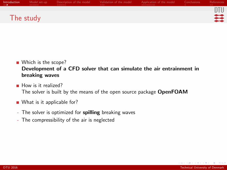
Which is the scope?Development of a CFD solver that can simulate the air entrainment inbreaking waves

How is it realized?The solver is built by the means of the open source package OpenFOAM

What is it applicable for?

- The solver is optimized for spilling breaking waves

- The compressibility of the air is neglected



Model set-up



Which is the main problem from the numerical point of view?

Wave breaking is an unsteady multiphase flow where a wide range of interfaciallength scales is involved

air

water

air bubbles

Wave propagation → O(m)! → scales larger thanthe grid size → Volume Of Fluid

Breaking event: entrainment of air bubbles →O(10−4 m)! → scales smaller than the grid size→ method for dispersed flow



Which method to handle the motion of bubbles?

Balachandar,2009:

St =τpτξ

=

(

2ρ+ 1

36

)(

1

1 + 0.15Re0.687p

)(

d

ξ

)2(ξ

η

)4/3

Assuming: ρ = 0.001, ξ = 0.01 m, η ≈ 1 · 10−5 m, d = [0.0006 0.0008 0.0010 0.00120.0016 0.0020 0.0025 0.0031 0.0039 0.0049 0.0062 0.0078 0.0099] m

100

101

102

103

0.001

0.2

1

d/η [-]

St[-]

Dusty gas

Equilibrium Eulerian

Eulerian

Lagrangian



A quick look at the multiphase Eulerian methodology

N-S equations discretized in a control volume with n phases inside → n equations forthe bulk of the volume + n − 1 jump conditions across interfaces among phases.

Equations are spatially averaged:

- phase fraction α stems

- the momentum transfer at the interface is not resolved and then needs to be modeledby a sub-grid term

∂(αiρi)

∂t+∇ · (αiρiui) = Si

∂(αiρiui)

∂t+∇ · (αiρiui ⊗ ui) = −αi∇p +∇ · (αiρiTi) + αiρig +Mi

Set of equations solved per each phase → 2n equations



How can the coupling be realized?

Coupling means that the VOF-like solver is combined with the multiphase Eulerianmethodology.

Which phases are involved?water + air above the free surface + n bubble classes = n+2!

Different couplings exist, two have been tried:

air bubbles

air

water

Eulerian framework

for all phases

Numerical sharpening and Mi

air bubbles

mixture

Eulerian for bubbles in the mixture

VOF for the mixture

Numerical sharpening



VOF with momentum transfer modeling at the free surface

”Glass of water” Propagation of a solitary wave

−4 −2 0 2 4 6 8

0

0.03

0.06

0.09

0.12

0.15

Surface

elevationfrom

SW

L[m

]x [m]

Instabilities at the free surface in both cases!



VOF without momentum transfer modeling at the free surface

water (w)continuous air (air)n classes

ρmixt =αwρw+αairρair

αw+αair

νmixt =αwνw+αairνair

αw+αair

n classesmixture (mixt)

Calculation of pressureand velocities (PISO algorithm)

Calculation of void fractions(MULES algorithm)

”Glass of water”

Main achievement: modeling of the momentum transfer between water andcontinuous air not needed anymore!



Description of the model



Governing equations

Averaged mass and momentum conservation equations:

∂(αiρi)

∂t+∇ · (αiρiui) = Si

∂(αiρiui)

∂t+∇ · (αiρiui ⊗ ui) = −αi∇p +∇ · (αiρiT

effi ) + αiρig +Mi

The n classes have the same density and viscosity but they have different diameter

Si and Mi represent mass transfer and interfacial forces among phases respectively



Effective stress tensor Teffi

By employing the eddy-viscosity approximation, the effective stress tensor is:

Teff = 2(νeffi ])

[

1

2(∇ui +∇uT

i )−1

3(∇ · ui)I

]

−2

3kiI

The effective viscosity of the mixture phase νeff is (Deen et al., 2001):

νeff = ν + νt + νBI

ν = νmixt and νt is the turbulent viscosity calculated by a dynamic Smagorinsky model

νBI is an extra-term accounting for the bubble-induced turbulence (Sato et al., 1975):

νBI = 0.6

n∑

i=1

αidi |ui − umixt |



Mass exchange among phases Si

Si = B+i + B−

i + C+i + C−

i + Ei + Di

Mass transfer among the n classes:- breakage → B+

i + B−i (Prinche et Blanch, 1990)

- coalescence → C+i + C−

i (Martinez-Bazan et al., 1999)

dj < di < dk

breakage

coalescence

Mass transfer between the dispersed bubbles and air-from air into the n classes → air entrainment → Ei

-from the n classes into air → degassing → Di

Degassing modeled as (Hansch et al., 2012):

Di = ϕairρiαi/ (at∆t)

where ∆t is the time step, at = 20 a constant and ϕair = 0.5tanh[100(αair − 0.5)] + 0.5



Air entrainment modeling

The air entrainment is reproduced by a sub-grid scale model (Derakhti and Kirby,2014):

Ei =cen

4π

ρmixt

σαmixt

(

f∆i∑n

i (di2 )

2f∆i

)

ǫsgs

- cen is a parameter which regulates the amount of entrained bubbles- fi is the size spectrum of the entrained bubbles (Deane and Stokes, 2002):

fi =

{

(di2)−

103 if (di

2) > 1 mm.

(di2 )− 3

2 if (di2 ) ≤ 1 mm.

- ∆i is the width of each bubble class

Bubbles are entrained at the free surface cells when ǫsgs is larger than a fixedthreshold!

ǫsgs is the rate of transfer of energy from the resolved to the sub-grid scales modeled byLES turbulence model:

ǫsgs = 2νt‖0.5(∇umixt +∇uTmixt)‖

2



Momentum transfer among phases Mi

Between every class and mixture phase:

Mi = MD,i +ML,i +MVM ,i +MTD,i

- Drag force MD,i =34ρmixtαmixtαiCD

‖ui−umixt‖(ui−umixt)di

- Lift force ML,i = −ρmixtαmixtαiCL(ui − umixt)× (∇× umixt)

- Virtual mass force MVM ,i = ρmixtαmixtαiCVM

(

Dumixt

Dt− Dui

Dt

)

- Turbulent dispersion force MTD,i = −34CD

ρmixt

di

(νt+νBI )Sb

‖ui − umixt‖∇αi

Between water and continuous air, i.e. at the free surface, the tension force isaccounted as (Brackbill et al., 1992):

Msurf ,i = σκ∇α (1)

σ = 0.0728 N/m and κ is the free surface curvature.



Free surface sharpening method

An additional term is added to the interface transport equations of water andcontinuous air:

∂(αiρi)

∂t+∇ · (αiρiui) +∇ · [ucαi(1− αi)] = Si

The ”compression velocity”uc compresses the interface counteracting the numericaldiffusion:

uc = min(C‖ur‖,max(‖ur‖))∇α

‖∇α‖

C is a coefficient that the user can specify and was taken as 1



Validation of the model



Bubble column of (Deen et al., 2001): simulation set-up

z

x

y

0.15 m

0.15

m

0.4

5 m

1.00 m

air

measurement point

(0,0,-0.20m)

init

ial w

ate

r le

vel

Uniform 3D hexaedral mesh of size 0.01 m

LES dynamic Smagorinsky model employed

Flow simulated for 600 s

Turbulence quantities time-averaged after the first 30 s.

Two different number of classes n:- n = 1 → di = 4 mm- n = 11 → di = [1.0 1.2 1.6 2 2.5 3.1 4.0 5.0 6.3 8 10]mm

Why this case? It resembles the motion of the bubbleplume in waves. The difference is that the air entrainmentis imposed by boundary conditions.



Bubble column of (Deen et al., 2001): results

−0.075−0.05−0.025 0 0.025 0.05 0.075−0.1

0

0.1

0.2

0.3

x [m]

uz,w

[ms−

1]

experimentn = 1n = 11

Mean water axial velocity

−0.075−0.05−0.025 0 0.025 0.05 0.075−0.1

−0.05

0

0.05

0.1

0.15

0.2

x [m]

√

u′2x,y,z,w

[ms−

1]

experiment√

u′2x,w

√

u′2y,w

√

u′2z,w

Mean water turbulence fluctuations

−0.075−0.05−0.025 0 0.025 0.05 0.0750

0.1

0.2

0.3

0.4

0.5

x [m]uz,air[m

s−1]

experimentn = 1

Mean air axial velocity

−0.075−0.05−0.025 0 0.025 0.05 0.075−0.01

0

0.01

0.02

0.03

x [m]

kw[m

2s−

2]

experimentn = 1n = 11

Mean turbulent kinetic energy

−0.075−0.05−0.025 0 0.025 0.05 0.0750

0.01

0.02

0.03

0.04

0.05

x [m]

αair[-]

n = 1n = 11

Mean gas hold-up

10−2

100

102

104

10−15

10−10

10−5

100

105

Frequency [Hz]

Spe

ctra

l den

sity

[m2 s

]

−5/3

−3

u′

x,w

u′

y,w

u′

z,w

Spectrum of turbulence



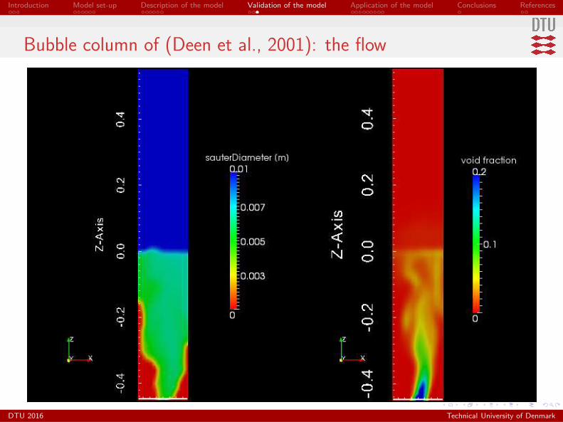
Bubble column of (Deen et al., 2001): the flow



Application of the model



An isolated unsteady spilling wave

Case set-up:

- Flume is 25 m long by 0.6 wide by 0.6 m high. Still water level at 0.4 m from theconstant bottom

- Breaking event by a dispersive focusing method:80 linear components of a JONSWAPspectrum (Tp = 1.7 s, Hs = 0.084 m, γ = 3.3.)

- Linear superposition at focusing point x = 15.0 m

Simulation:

- Quasi-uniform 3D mesh of size 0.0125 m

- Flow simulated for 25 s.

- LES dynamic Smagorinsky employed

- waves2Foam (Jacobsen et al., 2012) coupled with the model and used forwave generation



An isolated unsteady spilling wave: surface elevation

−5 −4 −3 −2 −1 0 1 2 3−0.2

−0.1

0

0.1

0.2

η[m

]

t∗ [-]

−5 −4 −3 −2 −1 0 1 2 3−0.2

−0.1

0

0.1

0.2

η[m

]

t∗ [-]

linearCFD

linearCFD

Upper: x=8 m. Lower: x = xb = 15.0 m

Simulated breaking point xb ≈ 15.0 m

Simulated breaking time tb ≈ 16.85 s

Period of highest wave Tc ≈ 1.6 s

t∗ =t − tob

Tc

Comparison reveals second order effects



An isolated unsteady spilling wave: bubble entrainment

Parameters cen and ǫsgs of the air entrainment model need to be calibrated. How?(Lamarre and Melville, 1991) measured void fraction in similar waves → cen = 20 andǫsgs = 0.01 m2 s−3

0 0.5 1 1.50

0.2

0.4

0.6

0.8

1

1.2

Vb /V

0 [−]

t∗ [-]

0 0.5 1 1.50

10

20

30

Ab /V

0 [−]

t∗ [-]

experiment7phases14phases

experiment7phases14phases

- Two simulations: 7 phases and 14 phases

- Volume per unit length of crest:

V b =

∫

A

αbH(αb − αbthld)dA

- Cross-sectional area:

Ab =

∫

A

H(αb − αbthld)dA



An isolated unsteady spilling wave: the bubble plume

As in study of (Rojas and Loewen, 2010), the roller moved downstream with a speed ≈100% of the celerity of the highest wave (Cc = Lc/Tc ≈ 1.8 m s−1) and the thicknessof the roller was around 5 cm.



An isolated spilling wave: impact on a cylinder

In the same domain a (slender) cylinder with a diameter D = 0.05 was placed at x =15.7 m (why? to let the plume develop!)

Computation of computed of in-line force without and with bubbles (7 phases)

No-slip condition for water velocity at the cylinder surface



An isolated spilling wave: impact without bubbles

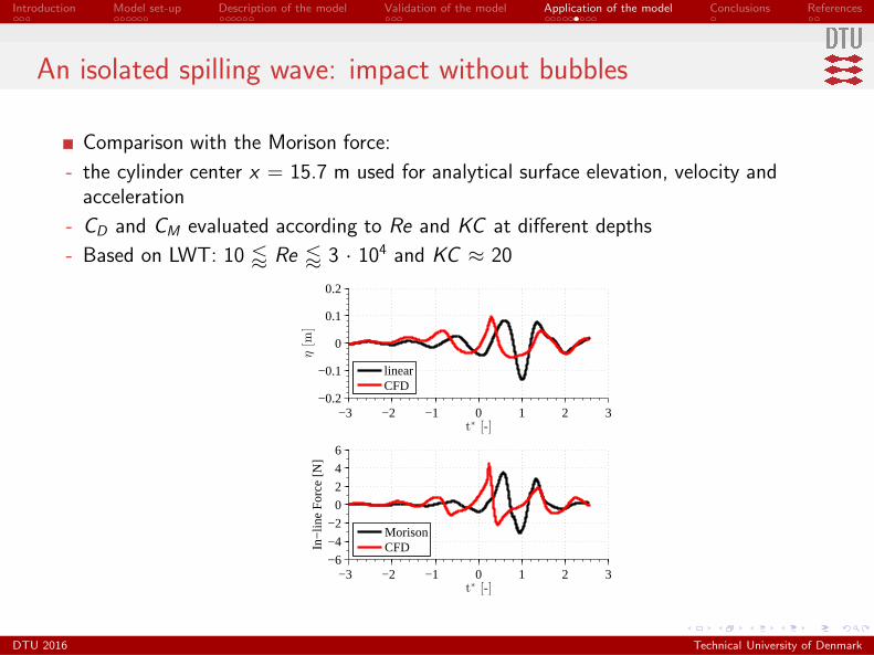
Comparison with the Morison force:

- the cylinder center x = 15.7 m used for analytical surface elevation, velocity andacceleration

- CD and CM evaluated according to Re and KC at different depths

- Based on LWT: 10 / Re / 3 · 104 and KC ≈ 20

−3 −2 −1 0 1 2 3−0.2

−0.1

0

0.1

0.2η[m

]

t∗ [-]

−3 −2 −1 0 1 2 3−6

−4

−2

0

2

4

6

In−

line

For

ce [N

]

t∗ [-]

linearCFD

MorisonCFD



An isolated spilling wave: impact with bubbles



An isolated spilling wave: impact without VS with bubbles

Differences are recognized at the interval 0.15 ≤ t∗ ≤ 0.4 when the bubble plumepassed over the cylinder

Largest differences are localized at around t = 0.25 t∗ when the volume of the bubbleplume was maximum

0 0.25 0.5 0.75 1 1.25 1.5−6

−4

−2

0

2

4

6In

−lin

e F

orce

[N]

t∗ [-]

0.1 0.15 0.2 0.25 0.3 0.35 0.4−6

−4

−2

0

2

4

6

In−

line

For

ce [N

]

t∗ [-]

CFD no bubblesCFD with bubbles

CFD no bubblesCFD with bubbles



The boundary layer around the cylinder

In the adopted model, the cell size must be larger the biggest bubble (≈ 1 cm usually)

For the highest Re - just near the roller! - separation and vortex shedding occur

The resolution of mesh around the cylinder may not be enough high to capture theseparation

- uniform current in the 3D flume

- Re = 2 · 104

- CD ≈ 1.3

0 10 20 30 40 500

0.5

1

1.5

2

2.5

3

t [s]

CD[-]

dynamic Smagorinskydynamic Smagorinsky with WFconstant Smagorinsky with vDDES



Conclusions



Main conclusions and on-going work

A CFD simulation of the entire breaking wave process involves interfacial length scalesboth smaller and larger than the grid size.

An Eulerian model coupled with a VOF-type interface capturing algorithm wasdeveloped to handle such multi-scale problem.

A bubble column flow was analyzed to test the momentum transfer modeling and theimplemented mass transfer formulations.

An isolated breaking wave generated by a dispersive focusing method was simulated totest the air entrainment model

The impact of the spilling wave on a slender cylinder was reproduced to estimate theeffect of bubbles on the exerted in-line force.

Further investigations are needed, especially concerning the flow around the cylinder.



References



References

References I

Balachandar S. 2009. A scaling analysis for point-particle approaches to turbulentmultiphase flows. Int. J. Multiphase Flow 35:801-10

Sato, Y., and Sekoguchi, K., 1975. ”Liquid velocity distribution in two-phase bubbleflow”. International Journal of Multiphase Flow, 2(1), pp. 79-95.

Martinez-Bazan, C., Montanes, J., and Lasheras, J., 1999. ”On the breakup of an airbubble injected into a fully developed turbulent flow. Part 1. Breakup frequency”.Journal of Fluid Mechanics, 401, pp. 183-207.

Martinez-Bazan, C., Montanes, J. L., and Lasheras, J., 1999. ”On the breakup of an airbubble injected into a fully developed turbulent flow. Part 2. Size PDF of the resultingdaughter bubbles”. Journal of Fluid Mechanics, 401, pp. 183-207.

Prince, M. J., and Blanch, H. W., 1990. ”Bubble Coalescence and Break-Up inAir-Sparged Bubble Columns”. AIChE Journal, 36(10), pp. 1485-1499.

Hansch, S., Lucas, D., Krepper, E., and Hohne, T., 2012. ”A multi-field two-fluidconcept for transitions between different scales of interfacial structures”. InternationalJournal of Multiphase Flow, 47, Dec., pp. 171-182.



References

References II

Derakhti, M., and Kirby, J. T., 2014. ”Bubble entrainment and liquid-bubble interactionunder unsteady breaking waves”. Journal of Fluid Mechanics, 761, Nov., pp. 464-506.

Deane, G. B., and Stokes, M. D., 2002. ”Scale dependence of bubble creationmechanisms in breaking waves.”. Nature, 418(6900), Aug., pp. 839-44.

Brackbill, J., Kothe, D., and Zemach, C., 1992. ”A continuum method for modelingsurface tension”. Journal of Computational Physics, 100, pp. 335-354.

Deen, N. G., Solberg, T., and Hjertager, B. H., 2001. ”Large eddy simulation of theGas Liquid flow in a square cross-sectioned bubble column”. Chemical EngineeringScience, 56, pp. 6341-6349.

Rojas, G., and Loewen, M. R., 2010. ”Void fraction measurements beneath plungingand spilling breaking waves”. J. Geophys. Res., 115(C8), p. C08001.


a coupled vof-eulerian multiphase cfd model to...

Documents