a counterexample for an optimal search-and-stop model

A Counterexample for an Optimal Search-And-Stop ModelAuthor(s): Y. C. KanSource: Operations Research, Vol. 22, No. 4 (Jul. - Aug., 1974), pp. 889-892Published by: INFORMSStable URL: http://www.jstor.org/stable/169965 .

Accessed: 09/05/2014 00:30

Your use of the JSTOR archive indicates your acceptance of the Terms & Conditions of Use, available at .http://www.jstor.org/page/info/about/policies/terms.jsp

.JSTOR is a not-for-profit service that helps scholars, researchers, and students discover, use, and build upon a wide range ofcontent in a trusted digital archive. We use information technology and tools to increase productivity and facilitate new formsof scholarship. For more information about JSTOR, please contact [email protected].

.

INFORMS is collaborating with JSTOR to digitize, preserve and extend access to Operations Research.

http://www.jstor.org

This content downloaded from 169.229.32.137 on Fri, 9 May 2014 00:30:54 AMAll use subject to JSTOR Terms and Conditions

http://www.jstor.org/action/showPublisher?publisherCode=informs

http://www.jstor.org/stable/169965?origin=JSTOR-pdf

http://www.jstor.org/page/info/about/policies/terms.jsp


Technical Notes

A Counterexample for an Optimal Search-and-Stop Model

Y. C. Kan

Faculte Universitaire Catholique de Mons, Mons, Belgium

(Received January 29, 1973)

The idea of policy regions is very useful in characterizing an optimal strategy for problems in dynamic programming. However, there are occasions when intuition suggests that an optimal strategy may be characterized by some structure of policy regions, and yet it is extremely difficult to prove or disprove this conjecture. This paper presents a counterexample showing an intuitive conjecture to be wrong.

C ONSIDER THE TYPE of optimal search-and-stop model introduced by Ross. 11, Let there be two boxes, and let pi? be the given prior probability that a ball is

hidden in box i, i= 1, 2, E Pi-= 1. A search of box i costs ci (ci>0) and finds the ball with probability ai if the ball is in this box. Assume that a reward R is earned if the ball is discovered. At the beginning of each time period t= 1, 2, -.-, a searcher may decide to search box 1 or box 2 or to stop searching. The objective is to find an optimal strategy to maximize the expected net reward (expected reward minus expected searching cost).

Let the state at any time be characterized by pi, i= 1, 2, where pi is the pos- terior probability that the ball is in box i at a certain time (or stage). Since there are only two boxes, the state at any time can be represented by a scalar p, where pl =p, p2= -p. Then the following results are due to Ross.

(i) At any time t, an optimal strategy either searches a box with maxi aipilci or else stops. In terms of the state p, this implies that there exists a number p*, 0? p < 1, such that, if p 2 p *, an optimal strategy either stops or else searches box 1; if p < p *, an optimal strategy either stops or else searches box 2. p* is determined by alp*/cI=a2(l -P*)/C2.

(ii) The stopping region So, defined as the set of states for which it is initially optimal to stop, is a convex region or an interval, since p is a scalar.

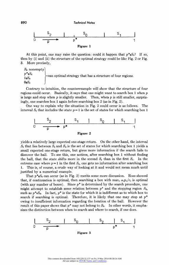
Let the horizontal coordinate be p, 0< p 1. Let S, i= 1, 2, be the set of states for which it is initially optimal to search box i. Then the structure of the optimal strategy is characterized by SO, SI, S2 on p. In fact, by (i) and (ii), if p*eSo, then there exists an optimal strategy that has a structure of at most three regions, as in Fig. 1.

This structure of three regions is intuitive. It says that, if p, the probability that the ball is in box 1, is large, then box 1 is searched; if p is small, meaning that P2= I-P iS large, then box 2 is searched. On the other hand, if p is somewhere in the middle, then stop.

889 OPERATIONS RESEARCH, Vol. 22, No. 4.



890 Technical Notes

l S 2 S0 I S1 0 - p 1

p Figure 1

At this point, one may raise the question: could it happen that p*4So? If so, then by (i) and (ii) the structure of the optimal strategy could be like Fig. 2 or Fig. 3. More precisely,

So nonempty

p4oSo t=an optimal strategy that has a structure of four regions.

14so )

Contrary to intuition, the counterexample will show that the structure of four regions could occur. Basically, it says that one might want to search box 1 when p is large and stop when p is slightly smaller. Then, where p is still smaller, surpris- ingly, one searches box 1 again before searching box 2 (as in Fig. 2).

One way to explain why the situation in Fig. 2 could occur is as follows. The interval SI that includes the state p = 1 is the set of states for which searching box 1

I 2 I s1 So I is 1 O -.-- p* 1

p Figure 2

yields a relatively large expected one-stage return. On the other hand, the interval Si that lies between So and S2 is the set of states for which searching box 1 yields a small expected one-stage return, but gives more information if the search fails to discover the ball. To see this, one notices, after searching box 1 without finding the ball, that the state shifts more in the second Si than in the first Si. In the extreme case where p= 1 in the first Si, one gets no information after searching box 1. This is, of course, a crude way of looking at it and would not mean much until justified by a numerical example.

That p*4So can occur (as in Fig. 2) merits some more discussion. Ross showed that, if continuation is optimal, then searching a box with maxi aipi/ci is optimal (with any number of boxes). Since p* is determined by the search procedure, one might attempt to establish some relation between p* and the stopping region So, such as p*ESo. In fact, p* is the state for which it is indifferent as to which box to search if searching is optimal. Therefore, it is likely that one may stop at p* owing to insufficient information regarding the location of the ball. However the result of this paper shows that p* may not belong to So. In other words, it empha- sizes the distinction between when to search and where to search, if one does.

I- S2 S0 I S2 1 I I 0 * 1

p Figure 3



Y. C. Kan 891

THE COUNTEREXAMPLE

A STRATEGY IS any sequence (or partial sequence) 6 = (61, *, 6k), where 6 E{ 1, 2} for i=1, * , s and sE{O, 1, 2, ** oo 3. The strategy 6 instructs the searcher to search box As at the ith stage and to stop searching if the object has not been found after the sth search. Now, s=O means that the searcher stops immediately, and s = cc means that he does not stop until he finds the ball.

For any strategy 6 and any state p, 0 < p _ 1, let f(p, 5) = the expected net reward (expected reward minus expected searching cost) incurred when p is the prior probability that the ball is in box 1 and strategy a is employed. Let f(p) =

supaf(p, b). Then, since So is the stopping region, So = { p :f(p) = O}. The following lemma will be used in the couilterexample. LEMMA. Let 5* be the strategy that searches at each stage a box with maxl,2 {Ja2P/CI,

a2 (1-p )/c23 until finding the ball. Then the existence of three strategies (5, (51 (52 and a value for p, 0 <p <1, satisfying the following conditions, implies the existence of an optimal strategy having a structure of four regions:f (1, 51) >, f(O, (50) >, f(p*, 62) >0o and f(p, 5*) <o for some p.

Proof. Now, f (1) f (1, 61) >0}1l So; f (O) >f(O, 50)>0o0oSo; and f (p*) >?

f(p*, 52) > 0p*SO. Suppose the structure of the optimal policy has no stopping region, i.e., the

optimal strategy never stops. Then clearly 5* is optimal for all p[O, 1], which implies f(p, 5*) ? Ofor all p. Therefore, f( (,5*) < Ofor some p implies that the stopping region So is not vacuous. It follows from (i) and (ii) that there exists an optimal strategy that has four regions.

It remains to find numerical values for the parameters so that the conditions in the Lemma are satisfied.

Let R=6.6, al=3/, a2 C1=1, c2=3. Let O 0?=keep on searching box 2 until finding the ball. 61 =keep on searching box 1 until finding the ball. 62 =search box 1, then box 2, and then stop. 63 =the sequence used by following *, given that the initial state is p*.

Let p(i) be the state of the process after ith stage, given that the initial state is p* and that 6* is used. At p*, ap*/c =a2(1 -p*)/c2. Hence, 6* says one may search either box 1 or box 2; i.e., 61 = 1 or 2. Suppose 61 = 1; then,

P* = (a2/C2)/(lal/cI+c2/c2) =2/11,

falP(') IC1]: [a2 (1 -P(1) ) /C21 (1- al) (a1P*1C1): [a2 (1- P*) IC21 = 1- al 1==6-2 = 2y

[Xalp(2)ICII: [a2 ( -p (2) )/C21 = (1 -al ) : (1 - a2) = (Y4): (Y2 )==>53= 2

[a1p(3)/C1I:[a2(1 --p(3))/C2I = (1 -al) :(1 -ca2)2= 1==M4 = 1 or 2=>p(3) =p*.

It follows that 63 can be a periodic sequence, namely, 6= 122, 122, * * . Consequently,

f(p*, 6*)=f(p*, 63)

-otsp*R- c, + (1- alP *) [ax2 (1 - P(1) )R -C2]

+ (1-alp*)[l-a2(1-p(l))I[a2(1l- p2))R-C21

+ (l-alP*)[1-a2(1-P())).[1a2(1-p(2))] .f(p*, 3).



892 Technical, Notes

Thanks to the recursive relation, one can compute f(p*, 6*) by substituting the numerical values of the parameters.

f(p*, 6*)=>-218/33=6.60-6.606<0,

f(1, bI)=R-ci/a,=6.6-Y3>0, f(O, 60)=R-c2/a2=6.6-6>0,

f(p*, 62)-=apl*R-cl+ (1-ap*)[ae(l-p(l))R-C2] = (24/44) (6.6-6.583 * )>0.

Thus, all the conditions in the Lemma are satisfied, and the counterexample is complete.

REFERENCES

1. R. BELLMAN, Dynamic Programming, Princeton University Press, Princeton, New Jersey, 1957.

2. W. BLACK, "Discrete Sequential Search," Information and Control 8, 159-162 (1965.) 3. M. CHEW, JR., "A Sequential Search Procedure," Ann. Math. Stat. 38, 494-502 (1967). 4. J. KADANE, "Discrete Search and the Neyman-Pearson Lemma," J. Math. Anal. Appl.

22, 156-171 (1968). 5 S. POLLOCK, "A Simple Model of Search for a Moving Target," Opns. Res. 18, 883-904

(1970). 6. S. Ross, "A Problem in Optimal Search and Stop," Opns. Res. 17, 985-992 (1969).

A Duality Theory for Convex Programming with

Set-Inclusive Constraints

A. L. Soyster

Temple University, Philadelphia, Pennsylvania

(Received June 25, 1973)

This paper extends the notion of convex programming with set-inclusive constraints as set forth by Soyster [Opns. Res. 21, 1154-1157 (1973)] by re- placing the objective vector c with a convex set C and formulating a dual problem. The primal problem to be considered is

sup finfc,,c c*x Ix1Kl+x2K2+? *xnKnCK(b), x j >O} (I)

where the sets {K31 are convex activity sets, K(b) is a polyhedral resource set, C is a convex set of objective vectors, and the binary operation + refers to addition of sets. Any feasible solution to the dual problem provides an upper bound to (I) and, at optimality conditions, the value of (I) is equal to the value of the dual. Furthermore, the optimal solution of the dual problem can be used to reduce (I) to an ordinary linear programming problem.

THE USUAL definition of a convex program involves the minimization of a convex function subject to a finite number of inequality constraints involving

convex functions. For example, suppose that f, q1, 92, g-, q are convex func-

OPERATIONS RESEARCH, Vol. 22, No. 4, July-August 1974



a counterexample for an optimal search-and-stop model

Documents