A Convex Relaxation for Approximate Global Optimization in SimultaneousLocalization and Mapping

David M. Rosen∗, Charles DuHadway†, and John J. Leonard∗

Abstract—Modern approaches to simultaneous localization andmapping (SLAM) formulate the inference problem as a high-dimensional but sparse nonconvex M-estimation, and then applygeneral first- or second-order smooth optimization methods torecover a local minimizer of the objective function. The perfor-mance of any such approach depends crucially upon initializingthe optimization algorithm near a good solution for the inferenceproblem, a condition that is often difficult or impossible toguarantee in practice. To address this limitation, in this paperwe present a formulation of the SLAM M-estimation with theproperty that, by expanding the feasible set of the estimation pro-gram, we obtain a convex relaxation whose solution approximatesthe globally optimal solution of the SLAM inference problem andcan be recovered using a smooth optimization method initializedat any feasible point. Our formulation thus provides a meansto obtain a high-quality solution to the SLAM problem withoutrequiring high-quality initialization.

I. INTRODUCTION

The ability to learn a map of an initially unknown environ-ment while simultaneously localizing within that map as it isbeing constructed (a procedure known as simultaneous local-ization and mapping (SLAM)) is a fundamental competencyin robotics [1]. Consequently, SLAM has been the focus of asustained research effort over the previous three decades, andthere now exist a variety of mature algorithms and softwarelibraries to solve this problem in practice (cf. [2]–[5]).

State-of-the-art approaches to SLAM typically formulate theinference problem as a high-dimensional but sparse nonconvexM-estimation [6], and then apply general first- or second-ordersmooth optimization methods to estimate a critical point of theobjective function. This approach admits the development ofstraightforward and fast inference algorithms, but its computa-tional expedience comes at the expense of robustness: specif-ically, the optimization methods that underpin these SLAMtechniques are usually only able to guarantee convergence toa first-order critical point of the objective (i.e. a local minimumor saddle point), rather than the globally optimal solution [7].This restriction to local rather than global solutions has severalimportant undesirable practical ramifications.

The most serious limitation is that the solution to whichany such method ultimately converges is determined by itsinitialization. This is particularly pernicious in the context ofSLAM, in which the combination of a high-dimensional statespace and significant nonlinearities in the objective function(due to e.g. the effects of rotational degrees of freedom in the

∗Computer Science and Artificial Intelligence Laboratory (CSAIL), Mas-sachusetts Institute of Technology, Cambridge, MA 02139, USA. Email:{dmrosen,jleonard}@mit.edu†Google Research, Mountain View, CA 94043, USA. Email:

duhadway@google.com

(a) Ground truth (b) Initial estimate

(c) Levenberg-Marquardt (d) Convex relaxation withsecond-stage LM refinement

Fig. 1. The effects of poor initialization on the SLAM estimation for thetorus11500 dataset (11500 6DOF poses, 22643 pose-pose measurements). (a):The ground truth map. (b): A poor (randomly sampled) initial estimate. (c):The solution obtained from Levenberg-Marquardt initialized with (b). (d): Thesolution obtained by first solving a convex relaxation of the original SLAMestimation problem (also initialized using (b)) to produce an approximation tothe globally optimal solution, and then refining this approximation in a second-stage optimization using Levenberg-Marquardt. This approach recovers aglobally consistent estimate in spite of the poor initialization.

estimated states or the use of nonlinear robust cost functions)can give rise to complex cost surfaces containing many localminima in which smooth optimization methods can becomeentrapped. The performance of any such SLAM technique thusdepends crucially upon initializing the back-end optimizationalgorithm with an estimate that is close to a good solution forthe inference task (Fig. 1). However, it is far from clear thatthis condition can always be satisfied in practice, especiallyin view of the fact that the entire point of solving the SLAMproblem is precisely to obtain such a high-quality estimate.

One general strategy for attacking challenging optimizationproblems of this type that has proven to be very successfulis convex relaxation. In this approach, the original problem ismodified in such a way as to produce a convex approximation(for which a globally optimal solution can be readily obtainedusing local smooth optimization techniques initialized at anyfeasible point [8]), whose solution then approximates a so-lution for the original problem. While theoretical bounds onthe approximation loss of such relaxations are often difficult to

produce (or turn out to be quite weak), a large body of numer-ical experience has shown that this approach often performsremarkably well in practice when applied to “typical” probleminstances (i.e., instances that are not artificially adversarial).

Motivated by this prior experience, in this paper we pro-pose a practical approach to global optimization in SLAMvia convex relaxation. Our approach formulates the SLAMproblem as an instance of M-estimation with the property that,by expanding the feasible set of the estimation program, weobtain a convex relaxation whose globally optimal solution canbe computed efficiently in practice; by projecting this solutiononto the feasible set of the original program, we thereby obtaina good approximation of the global solution to the originalSLAM M-estimation problem which is suitable for subsequentrefinement with a local smooth optimization technique. Ourapproach thus provides a means to obtain a good estimate forthe globally optimal solution of the SLAM problem withoutthe need to supply a high-quality initialization.

II. THE SLAM M-ESTIMATION AND ITS CONVEXRELAXATION

A. Notation and mathematical preliminaries

Our development will make frequent use of the geometryof the special orthogonal and special Euclidean groups andtheir realizations as subsets of linear spaces. To that end,in this subsection we briefly establish some notational andmathematical preliminaries that will be useful in the sequel.

We let [n] , {1, 2, . . . , n} denote the first n positiveintegers and R≥0 the nonnegative real numbers. We denoteby SO(n) the realization of the special orthogonal group asthe set of n× n orthogonal matrices with +1 determinant:

SO(n) , {R ∈ Rn×n |RTR = RRT = I, detR = 1}. (1)

Similarly, we will denote by SE(n) the realization of thespecial Euclidean group1 as the semidirect product

SE(n) , Rn o SO(n) (2)

under the group operation ⊕:

⊕ : SE(n)× SE(n)→ SE(n)

(t1,R1)⊕ (t2, R2) = (t1 +R1t2, R1R2).(3)

SE(n) also has a group action2 • on Rn given by:

• : SE(n)× Rn → Rn

(t, R) • x = Rx+ t.(4)

Finally, we denote by V (n) the real vector space containingthe realization (1)–(3) of SE(n):

V (n) , Rn × Rn×n. (5)

1 This Lie group models the set of robot poses in n-dimensional Euclideanspace under the operation of odometric composition.

2 This action transforms a point whose coordinates x ∈ Rn are specified inthe global coordinate frame (the frame of the identity pose (0, I) ∈ SE(n))to coordinates in the frame associated with the robot pose (t, R) ∈ SE(n).

B. The SLAM M-estimation problem

In this section we provide a brief review of the pose-and-landmark SLAM inference problem; interested readers areencouraged to consult [1], [9] for a more detailed presentation.

We consider a robot attempting to learn a map of someinitially unknown environment. As the robot explores, it movesthrough some sequence of poses p1, . . . , pnp ∈ SE(n) in theenvironment while observing some collection of landmarksl1, . . . , lnl

∈ Rn for n ∈ {2, 3}. We assume that the robotis able to collect noisy observations zij ∈ SE(n) of pose pjin the coordinate system of pose pi for some subset of pairs(i, j) ∈ P ⊂ [np] × [np], and noisy observations lik ∈ Rn ofthe position of landmark lk in the coordinate frame of pose pifor some subset of pairs (i, k) ∈ L ⊂ [np]× [nl]. The goal isthen to estimate the configuration of the states

X ,(p1, . . . , pnp , l1, . . . , lnl

)∈

,F︷ ︸︸ ︷(SE(n))

np × (Rn)nl (6)

(i.e. the poses pi and landmarks lk) given the observations

Z , {zij | (i, j) ∈ P} ∪{lik | (i, k) ∈ L

}. (7)

Now in principle, the poses pi, landmarks lk, and observa-tions zij and lik should satisfy the measurement equations:

pj = pi ⊕ zij (8a)lk = pi • lik (8b)

for all (i, j) ∈ P and all (i, k) ∈ L; however, becausethe observations zij and lik are corrupted by sensor noise,equations (8) are generally inconsistent in the sense that nochoice of states X in (6) can satisfy them all simultaneously.Thus, in practice, the SLAM inference problem is solved viaM-estimation [6]: we define a set of cost functions

cij(pi, pj) : SE(n)× SE(n)→ R≥0 ∀(i, j) ∈ P (9a)cik(pi, lk) : SE(n)× Rn → R≥0 ∀(i, k) ∈ L (9b)

that penalize the failure of equations (8) to hold, and thendefine an optimal state estimate X∗ ∈ F to be one thatminimizes the cumulative cost of the penalties (9):

X∗ = argminX∈F

,f(X)︷ ︸︸ ︷∑(i,j)∈P

cij(pi, pj) +∑

(i,k)∈L

cik(pi, lk)

subject to p1 = (0, I).

(10)

In practice, the cost functions cij and cik in (9) and (10) areusually chosen as negative log-likelihoods for some assumedmeasurement models pij(zij |pi, pj) and pik(lik|pi, lk) (i.e. forsome assumed distribution on the measurement noise affectingthe observations zij and lik), in which case the M-estimationin (10) is actually a maximum-likelihood estimation. Forexample, the most common formulation of the SLAM problemassumes additive mean-zero Gaussian noise models, for which

the corresponding negative log-likelihood functions are:

cGij(pi, pj) = ‖ωij‖2ΣRij

+∥∥tij −RT

i (tj − ti)∥∥2

Σtij

(11a)

cGik(pi, lk) =∥∥lik −RT

i (lk − ti)∥∥2

Σik, (11b)

where ‖x‖Σ ,√xT Σ−1x is the norm corresponding to the

Mahalanobis distance, ΣRij ,Σ

tij ,Σik � 0 are the noise covari-

ance matrices, and ωij ∈ R3 is the axis-angle representationfor the rotational measurement residual RT

i RjRTij ∈ SO(3)

(that is, ωij satisfies [ωij ]× = log(RTi RjR

Tij)). However, for

our purposes it will be convenient to admit more general (i.e.non-probabilistic) cost functions in the sequel.

C. Convex relaxation of the SLAM M-estimation

In general, the SLAM M-estimation (10) is a high-dimensional nonconvex nonlinear program, and thus can bequite challenging to solve using smooth numerical optimiza-tion methods [7]. To address this difficulty, in this sectionwe describe a special class of instances of (10) that admitsa straightforward convex relaxation, whose globally optimalsolution can be found using these techniques.

Our approach is based upon the observation that if wemodel the (abstract) special Euclidean group SE(n) using therealization defined in (1)–(3), then the feasible set F for theSLAM M-estimation (10) embeds into the linear space

S , (V (n))np × (Rn)nl . (12)

The embedding F ↪→ S provides us with a means to“convexify” F by enlarging it to its convex hull within theambient linear space S. If we additionally select the objectivefunction f in (10) such that it has a convex extension definedover the convex hull of F , then the relaxation of (10) obtainedby extending F to convF within S will be a convex program.

1) Selecting the cost functions: We wish to determine costfunctions cij and cik in (9) that have convex extensions overthe convex hulls of their respective domains. Given that we areworking within an ambient linear space, a natural cost functionto consider is a norm: these are convex by definition, andthe metric topology that they generate is the usual Euclideantopology (so that the “costs” they assign agree with the usualnotion of “closeness” in these spaces). By virtue of (3) and(8a), we might therefore consider the pose-pose measurementerror functions:

eRij(pi, pj) = ‖Rj −RiRij‖, (13a)

etij(pi, pj) = ‖tj − (ti +Ritij)‖, (13b)

for (i, j) ∈ P , where ‖·‖ denotes any choice of matrix orvector norm in (13a) and (13b), respectively; these functionsthen serve to quantify the disagreement between the rotationaland translational components of the left- and right-hand sidesof (8a). Similarly, by virtue of (4) and (8b), we might considera pose-landmark measurement error function of the form

eik(pi, lk) = ‖lk − (ti +Ri lik)‖, (14)

for (i, k) ∈ L, where ‖·‖ is any vector norm. Finally, in orderto implement a robust M-estimation, we might wish to allow

the possibility of composing the error functions in (13) and(14) with robust cost functions ρ : R≥0 → R≥0 [6]. Thus, wewill consider cost functions cij and cik of the form

cij(pi, pj) = ρRij(‖Rj −RiRij‖

)+ ρtij (‖tj − (ti +Ritij)‖)

(15a)

cik(pi, lk) = ρik(‖lk − (ti +Ri lik)‖

). (15b)

2) Constructing the convex relaxation: Here we establishour main result: a prescription for constructing a convexrelaxation of the SLAM M-estimation program (10).

Lemma 1. Let C be a convex set, f : C → R≥0 a convexfunction on C, and g : R≥0 → R≥0 a convex and nonde-creasing function on the nonnegative real numbers. Then thecomposition g ◦ f : C → R≥0 is also convex.

Proof: Let x1, x2 ∈ C and λ ∈ [0, 1]. Then

f(λx1 + (1− λ)x2) ≤ λf(x1) + (1− λ)f(x2) (16)

by the convexity of f . Since g is nondecreasing and convex,then (16) implies

g(f(λx1 + (1− λ)x2)) ≤ g(λf(x1) + (1− λ)f(x2))

≤ λg(f(x1)) + (1− λ)g(f(x2))

which is the desired inequality.

Theorem 1 (Convex relaxation of the SLAM M-estimation).Let cij and cik be the cost functions defined in (15) withρRij , ρ

tij , ρik : R≥0 → R≥0 convex nondecreasing functions for

all (i, j) ∈ P and (i, k) ∈ L, and let

C(n) , convSE(n) = Rn × convSO(n) (17a)

F , convF = (C(n))np × (Rn)nl (17b)

denote the convex hulls of SE(n) in V (n) and F in S,respectively. Then the objective function f : F → R≥0 definedin (10) extends to a convex function f : F → R≥0, andthe relaxation obtained from the SLAM M-estimation (10) byextending F to F:

X∗ = argminX∈F

f(X)

subject to p1 = (0, I)(18)

is a convex program.

Proof: The functions eRij , etij , and eik defined in equations(13)–(14) are compositions of linear inner functions withconvex outer functions (the norms), and are therefore convex(cf. [8, Sec. 3.2]); Lemma 1 thus guarantees that the costfunctions cij = ρRij ◦ eRij +ρtij ◦ etij and cik = ρik ◦ eik definedin (15) are convex, and therefore so is their sum f in (18)(recall (10)). We also observe that the feasible set of (18) isthe intersection of the convex set F in (17b) with the affineset determined by the constraint p1 = (0, I), and is thereforealso convex. Problem (18) is thus a convex program.

c

-1 0 1

s

-1

-0.5

0

0.5

1

0

2

4

6

8

(a) cRij(Ri, Rj) on SO(2)

c

-1 0 1

s

-0.5

0

0.5

1

0

2

4

6

8

(b) cRij(Ri, Rj) on convSO(2)

Fig. 2. Constructing the convex relaxation (18). (a): This figure plotsthe value of the rotational cost function cRij(Ri, Rj) defined in (19) as afunction of Ri ∈ SO(2) for αij = 1 and Rj = Rij = I2, using therealization SO(2) = {( c −s

s c ) | c2 + s2 = 1} ⊂ R2×2 described in(1). (b): The rotational cost cRij(Ri, Rj) shown in (a) extends to a convexfunction cRij(Ri, Rj) for Ri, Rj ∈ convSO(2), where the set convSO(2)is characterized explicitly by (20). The construction for SO(3) using (19)and (21) is analogous.

D. The relation between the convex relaxation and the stan-dard maximum-likelihood formulation of SLAM

The standard formulation of the SLAM problem (10) derivesthe cost functions (11) from an assumed Gaussian noise model,whereas our selection of the cost functions (13)–(15) wasprimarily motivated by a desire to obtain a convex objective for(18). It may therefore not be immediately clear how these twomodels relate, or whether the objective f in (18) constructedfrom (13)–(15) carries a natural interpretation in the same waythat a negative log-likelihood objective does. To that end, herewe briefly describe a specific choice of the cost functions (15)that act as pointwise upper bounds on the standard negativelog-likelihood cost functions (11) for all X ∈ F . We presentthe following theorem without proof, in the interest of brevity:

Theorem 2. For the following choice of cost functions (15):

cij(pi, pj) =

cRij(Ri,Rj)︷ ︸︸ ︷αij

∥∥Rj −RiRij

∥∥2

F+

ctij(pi,pj)︷ ︸︸ ︷βij ‖tj − (ti +Ritij)‖22

cik(pi, lk) = γij∥∥lk − (ti +Ri lik)

∥∥2

2(19)

where ‖·‖F is the Frobenius norm and ‖·‖2 is the usualEuclidean norm, it holds that cGij(pi, pj) ≤ cij(pi, pj) andcGik(pi, lk) ≤ cik(pi, lk) for all pi, pj ∈ SE(3) and lk ∈ R3

provided that

αij ≥π2

4λmin(ΣRij), βij ≥

1

λmin(Σtij), γij ≥

1

λmin(Σik).

The practical import of Theorem 2 is that it shows howto construct a specific class of admissible cost functions (15)for the convex relaxation (18) in such a way that minimizingthe convex objective f (as the relaxation (18) attempts to do)still “does the right thing” with respect to the usual Gaussianmaximum-likelihood formulation of the SLAM problem. Fig.2 illustrates the convex relaxation (18) obtained by using thecost functions (19) for the case of mapping in two dimensions.

III. APPROXIMATE GLOBAL OPTIMIZATION IN SLAMUSING THE CONVEX RELAXATION

In this section we discuss several practical aspects of solvingthe convex relaxation (18) and extracting from it an approxi-mate global solution of the original SLAM M-estimation (10).

Our point of departure (in Section III-A) is the observationthat the feasible set for the program (18) has a convenient spec-trahedral description (i.e. it can be expressed as the solutionset for a linear matrix inequality [10]). We show in SectionIII-B how to exploit this description (in the form of log-determinant barrier functions) to enable the implementation ofa fast second-order interior-point optimization method [7] tosolve the relaxation (18) efficiently in practice, and discussseveral of the computational advantages that this approachaffords. Finally, having obtained a global solution X∗ tothe convex relaxation (18) using this interior-point technique,we describe in Section III-C a simple but effective roundingprocedure to extract from X∗ a good initial estimate X for theglobal minimizer of the original SLAM M-estimation (10).

A. Spectrahedral description of convSO(n)

In order to implement the optimization (18) in practice, itis necessary to have a computational means of testing formembership in the feasible set F (in particular, of testing formembership in convSO(n) in (17a)). Fortunately, a suitablecriterion is provided by the following theorem due to Saun-derson, Parrilo and Willsky [11]:

Theorem 3 (Spectrahedral description of convSO(n)). Theconvex hull of SO(n) is a spectrahedron for all n ∈ N.For the special cases n = 2 and n = 3, the correspondingspectrahedral descriptions are given explicitly by equations(20) and (21):

convSO(2) =

R =

[c −ss c

]∈ R2×2 :

[1 + c ss 1− c

]︸ ︷︷ ︸

,A2(R)

� 0

. (20)

By means of Theorem 3, we can rewrite (18) as:

X∗ = argminX∈S

f(X)

subject to p1 = (0, I)

An(Ri) � 0 ∀i = 2, . . . , np

(22)

where An is the linear matrix operator defined in (20) or (21).Program (22) is a constrained convex optimization problem,

but in contrast to the usual (scalar) equality and inequality con-straints that one most commonly encounters in mathematicalprogramming, the constraints appearing in (22) are positivesemidefiniteness constraints; they require that the eigenvaluesof the (symmetric) matrices An(Ri) be nonnegative. As thereis in general no closed-form algebraic solution for the eigen-values of a matrix in terms of its elements, it may not beimmediately clear how one can effectively enforce constraintsof this sort when designing a numerical optimization method tosolve (22) in practice; we describe a suitable technique basedupon interior-point methods in the next subsection.

convSO(3) =

R ∈ R3×3 :

1− R11 − R22 + R33 R13 + R31 R12 − R21 R23 + R32

R13 + R31 1 + R11 − R22 − R33 R23 − R32 R12 + R21

R12 − R21 R23 − R32 1 + R11 + R22 + R33 R31 − R13

R23 + R32 R12 + R21 R31 − R13 1− R11 + R22 − R33

︸ ︷︷ ︸

,A3(R)

� 0

(21)

B. Solving the convex relaxation

In this subsection we describe a computationally efficientoptimization method for solving large-scale but sparse prob-lems of the form (22) effectively in practice. Our approach isbased upon exploiting properties of the class of interior-pointmethods for nonlinear programming [7] to enable the replace-ment of each positive semidefiniteness constraint An(Ri) � 0in (22) with an inequality constraint of the form c(Ri) ≥ 0for a scalar-valued function c(·).

1) Interior-point methods for nonlinear programming:Interior-point methods for nonlinear programming aim to solveconstrained optimization problems of the form

minimizex∈Rd

f(x) subject to

{ci(x) = 0, i ∈ E ,ci(x) ≥ 0, i ∈ I,

(23)

(where f, ci : Rd → R are real-valued, continuously-differentiable functions on Rd and E and I are disjoint finiteindex sets of equality and inequality constraints, respectively)by approximating a solution x∗ of (23) using the first compo-nent x of a solution (x, s) to the corresponding logarithmicbarrier program:

minimize(x,s)∈Rd×R|I|

f(x)− µ∑i∈I

log si

subject to

{ci(x) = 0, i ∈ E ,ci(x) = si, i ∈ I,

(24)

where µ > 0 is called the barrier parameter. Notice thatthe inequality constraints in the original nonlinear program(23) have been replaced in (24) by equalities involving theslack variables s ∈ R|I|. While this requires that si ≥ 0 forall i ∈ I in order for x to be feasible in (23), observe thatwe needn’t explicitly enforce this condition in (24); the factthat limsi→0+ − log si = +∞ together with the second setof equality constraints in (24) prevents the solutions x fromencroaching on the boundary of the feasible set of (23). Inthis way, the logarithmic terms in the objective in (24) act asa “barrier” that serves to keep the estimates x in the interior ofthe feasible set of the original program. While the estimate xarising from (24) will thus generally not coincide exactly witha solution x∗ of (23), one can show that x→ x∗ as µ→ 0+.Thus, in this approach the strategy is to solve a sequence ofbarrier problems of the form (24) for decreasing values of µ;since each of these barrier programs is an equality-constrainedoptimization, it can in turn be solved directly using the usualmethod of Lagrange multipliers [7].

2) Enforcing positive semidefiniteness constraints withinterior-point methods: Given a symmetric matrix S ∈ Rn×n,the condition that S � 0 is equivalent to the condition thateach of S’s (real) eigenvalues is nonnegative: λi(S) ≥ 0for i = 1, . . . , n. Now although there is in general noclosed-form algebraic solution to compute the eigenvaluesλi(S) as a function of S’s elements, it is nevertheless stillpossible to enforce the nonnegativity conditions λi(S) ≥ 0when performing numerical optimization with an interior-pointmethod by enforcing a clever (scalar) inequality constraint ofthe form c(S) ≥ 0.

Recall that the determinant of a matrix is the product of thatmatrix’s eigenvalues:

det(S) =

n∏i=1

λi(S). (25)

Consider enforcing a constraint of the form det(S) ≥ 0 whenapplying an interior-point method; the barrier term in thecorresponding logarithmic barrier program (24) is then:

− µ log det(S) = −µ log

(n∏

i=1

λi(S)

)= −µ

n∑i=1

log λi(S).

(26)But now observe that the right-hand side of (26) is preciselythe barrier term associated with the system of inequalities:

λi(S) ≥ 0 ∀i = 1, . . . , n. (27)

Equation (26) thus implies that a positive semidefinitenessconstraint of the form S � 0 can be replaced with a scalarconstraint of the form det(S) ≥ 0 when solving nonlinearprograms using an interior-point method, provided that thealgorithm is initialized with a strictly feasible starting pointS(0) � 0; in that case, the fact that λi(S(0)) > 0 for alli = 1, . . . , n by construction, together with the presence of thebarrier term −µ log det(S) in the logarithmic barrier program(24) (which prevents det(S(k)) → 0, i.e., prevents any ofthe λi(S

(k)) from changing sign during the optimization),ensures that every iterate S(k) likewise satisfies S(k) � 0.(As an aside, this observation forms the basis for the class ofcentral path-following interior-point methods for semidefiniteprogramming; cf. [10, Sec. 4].)

3) Practical implementation of the optimization: In lightof (23)–(27), we can solve (22) by applying an interior-pointmethod to the program

X∗ = argminX∈S

f(X)

subject to p1 = (0, I)

det(An(Ri)) ≥ 0 ∀i = 2, . . . , np

(28)

provided that the algorithm is initialized with a strictly feasiblestarting point (i.e. a point X(0) for which p1 = (0, I) andAn(R

(0)i ) � 0 for i = 2, . . . , n). This is the approach that we

will implement to solve (18) in practice.4) Computational considerations: To close this subsection,

we briefly highlight some of the attractive computationalproperties of the optimization approach described above.

Interior-point methods are a state-of-the-art class of accu-rate, high-speed techniques for solving large-scale nonlinearprograms, and enjoy excellent global convergence and numer-ical robustness properties [7], [12]. Furthermore, the fact thatthe constraints in (28) involve only unary functions of the gen-eralized orientations Ri means that the block-sparsity patternof the Hessian of the Lagrangian of the barrier programs (24)coincides (after substitution to eliminate the slack variables)with that of the Hessian of f(X) in (10) alone. Consequently,we expect the computational complexity of solving (28) usingan interior-point method based upon the exact (i.e. second-order) Newton step (cf. [13], [14], among others) will scalegracefully to problem sizes typical of those addressed by state-of-the-art least-squares methods for SLAM [3]–[5]. Solvingprogram (28) using interior-point methods thus provides anumerically robust and computationally efficient approach toobtain solutions X∗ of the convex relaxation (18).

C. Rounding the solution of the relaxed program

The convex relaxation (18) is obtained from the originalM-estimation (10) by expanding the original feasible set toits convex hull (more precisely, by expanding the feasibleset SO(n) for the pose orientation estimates to its convexhull convSO(n), as shown in Fig. 2). While this is desirablefor the computational advantages that convex programmingaffords, it also means that the solution X∗ of (18) willgenerally not lie in the feasible set for the original program(10); consequently, we must provide a method for transforminga solution X∗ of (18) into a feasible point for (10), a procedureknown as rounding.

In this case, since the objective functions for the originalprogram (10) and its convex relaxation (18) are actuallyidentical, we would like to design a rounding method thatperturbs the solution X∗ of (18) as little as is possible (in somesense) in order to restore feasibility in (10). Thus, one naturalway to round X∗ is by replacing each generalized orientationestimate R∗i ∈ convSO(n) with the nearest (in some sense)valid rotation matrix; i.e., we first define a rounding procedure

πR : convSO(n)→ SO(n)

πR(R) ∈ argminR∈SO(n)

‖R− R‖ (29)

that sends each R∗i to a closest rotation matrix in some norm‖·‖, and then define a rounding procedure π : F → F forX∗ that simply fixes all translational estimates and sendseach generalized orientation estimate Ri to one of its nearestrotation matrices πR(Ri):

π(p1, . . . , pnp , l1, . . . , lnl) = (p1, . . . , pnp , l1, . . . , lnl

) (30)

wherepi = (ti, πR(Ri)) ∀i ∈ [np]. (31)

Rounding procedures of the form (29) have been studiedpreviously, and there exist straightforward and efficient meth-ods to compute the mapping πR(·) (based upon the singularvalue decomposition [15] of R) for the special case in whichthe norm ‖·‖ in (29) is the Frobenius norm [16].

IV. RELATED WORK

The formulation of the SLAM inference problem as aninstance of the M-estimation (10) is originally due to Lu &Milios [17], who proposed the use of nonconvex negativelog-likelihood cost functions similar to (11); this formulationremains the basis for current state-of-the-art SLAM techniques(e.g. [2]–[5]), with most modern algorithms differing princi-pally only in how the optimization problem (10) is solved.

The most common approach is to use an approximate New-ton least-squares method (as in [3]–[5]) or gradient descent(as in [2]) to estimate a local minimizer of (10); however, asthese methods only guarantee convergence to local minima,the performance of this approach depends crucially uponinitializing the back-end optimization algorithm near a goodsolution for the inference problem. While there has been someprior work focused specifically on improving the robustnessof local search methods for optimization in SLAM withrespect to poor initialization (e.g. the development of improvedinitialization procedures [18] or reparameterizations of thestate space intended to broaden the basins of attraction ofgood solutions [2], [19]), ultimately these methods still dependupon identifying a good initialization for some nonconvex op-timization using either random sampling or a greedy kinematicexpansion along the edges of a spanning tree through thenetwork of measurements.

Alternatively, some recent work aims to avoid the brittlenessof smooth local optimization methods with respect to poorinitialization through the use of convex relaxations in a spiritsimilar to our own. One notable example is [20], whichguarantees the recovery of the globally optimal orientationestimates in the 2D pose-graph SLAM problem with high(user-selectable) probability; however, this approach dependsupon the identification SO(2) ∼= R/2πZ, and so appears tobe limited to the 2-dimensional case. Another recent methodsimilar to our own is [21], which formulates a specific in-stance of the convex relaxation (10) to solve the pointcloudregistration problem; our approach can be be thought of as anextension of this work from the special case of single-poseestimation based on pose-landmark observations to the moregeneral pose-and-landmark SLAM problem.

In practice, the convex relaxation (18) can be thought ofas an advanced initialization procedure that improves uponprior work by fusing information from all of the availablemeasurements Z to produce X∗ (rather than only a subsetcorresponding to the edges of some spanning tree in themeasurement network). We thus expect our approach to beparticularly advantageous versus prior techniques in cases

where the accumulated uncertainty along any single paththrough the network of measurements is high (e.g. high-noisescenarios or networks with deep spanning trees).

V. EXPERIMENTAL RESULTS

In this section we illustrate the performance of the ap-proximate global optimization method of Section III on twoclasses of standard pose-graph SLAM benchmarks, usingthe performance of the standard least-squares approach as abaseline for comparison.

Our test sets for these experiments consist of 100 randomly-sampled instances of the City and sphere2500 datasets. Weprocess each dataset twice: once using the usual least-squaresSLAM formulation, and a second time using our two-stageprocedure, in which we first find a minimizer X∗ of the convexrelaxation (18) (using the cost functions defined in (19)) bysolving (28), compute the rounded estimate X = π(X∗), andthen use X to initialize a second-stage local refinement usingthe standard least-squares SLAM formulation. In both caseswe initialize the first-stage optimization methods using theodometric initialization.

All experiments were run on a desktop with Intel XeonX5660 2.80 GHz processor. The convex optimization (28)was implemented in MATLAB using the fmincon interior-point method (which is itself an implementation of KNITRO,a high-quality interior-point trust-region method for large-scale nonlinear programming [13], [14]). The least-squaresminimizations in both cases were performed using the imple-mentation of Levenberg-Marquardt available in the GTSAMlibrary3 with the default settings, so any differences in thequality of the final estimates produced by these two approachesare due solely to the effect of refining the initialization usingthe convex relaxation (18).

A. Datasets

1) City datasets: In this experiment we evaluate the twoapproaches on the City problem, which simulates a robottraversing a 2D “grid world”; like the well-known Manhattanworld [19], this problem is designed to be challenging forlocal optimization methods to solve given poor initial estimates(for example, those obtained by composing long chains ofodometric measurements). Our test ensemble consists of 100randomly-sampled problem instances, each with 3908–4285poses and 7894–10195 pose-pose measurements. Results fromthis experiment are summarized in Table I; a representativeinstance from the test set is shown in Fig. 3.

2) sphere2500 datasets: We next evaluate the two methodson a high-noise version of the sphere2500 problem, a standard3D pose-graph SLAM benchmark. Our test ensemble consistsof 100 randomly-sampled problem instances, each with 2500poses and 4949 pose-pose measurements. Results from this ex-periment are summarized in Table II; a representative instancefrom the test set is shown in Fig. 3.

3The GTSAM Library (version 2.1.0), available through https://research.cc.gatech.edu/borg/sites/edu.borg/files/downloads/gtsam-2.1.0.tgz

(a) Ground truth (b) Odometric initialization

(c) Levenberg-Marquardt (d) Convex relaxation withsecond-stage LM refinement

Fig. 3. A representative instance of the City datasets (4269 poses, 8861measurements). (a): The ground truth map. (b): The odometric initializationfor this example (objective function value 1.238 E8). (c): The solutionobtained by Levenberg-Marquardt using the odometric initialization (6.887E7). (d): The solution obtained using the two-stage procedure of Section III(6.864 E3); this is the same solution obtained when initializing Levenberg-Marquardt with the ground truth (a). Note that the objective function values forboth (c) and (d) are within ±6% of the median values for the correspondingmethods reported in Table I.

B. Discussion

We can see from Tables I and II that the convex relaxationapproach significantly outperformed the standard least-squaresapproach on these examples; evidently the accumulated errorsin the odometric initializations were sufficient to prevent thelocal search performed by Levenberg-Marquardt from recover-ing good solutions to the inference problem in most cases. Incontrast, the two-stage convex relaxation approach consistentlyfinds good solutions to the inference task; indeed, the fact that(18) is convex implies that the solution X = π(X∗) used toinitialize the second stage refinement is completely immune tothe effects of the accumulated error in the odometric (or anyother) initialization for (18).

Of course, the enhanced performance of the two-stageapproach of Section III versus the standard least-squares ap-proach comes at the expense of additional computation (specif-ically, the additional computation needed to solve program(28) before applying the second-stage refinement). However,the timing results in Tables I and II show that this additionaloverhead is not a serious limitation to the effective use of themethod (in agreement with the analysis of Section III-B3), andis well-compensated by the gain in solution quality.

VI. CONCLUSION

In this paper we proposed a practical method for approxi-mating the globally optimal solution of the SLAM inferenceproblem that does not require initialization with a high-qualityestimate. Our approach is based upon a novel formulation ofthe SLAM M-estimation with the property that, by expandingthe feasible set of the estimation program, we obtain a convex

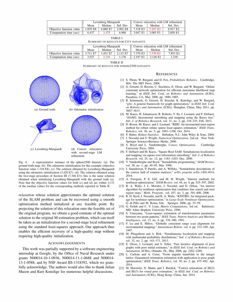
Levenberg-Marquardt Convex relaxation with LM refinementMean Median Std. Dev. Mean Median Std. Dev.

Objective function value 1.839 E8 6.880 E7 2.902 E8 7.318 E3 7.247 E3 6.917 E2Computation time (sec) 6.437 3.475 6.968 3.047 E1 3.085 E1 2.850 E1

TABLE ISUMMARY OF RESULTS FOR CITY DATASETS

Levenberg-Marquardt Convex relaxation with LM refinementMean Median Std. Dev. Mean Median Std. Dev.

Objective function value 3.711 E7 3.451 E7 2.115 E7 7.370 E3 7.370 E3 7.853 E1Computation time (sec) 3.527 3.316 1.176 2.197 E1 2.126 E1 1.210

TABLE IISUMMARY OF RESULTS FOR SPHERE2500 DATASETS

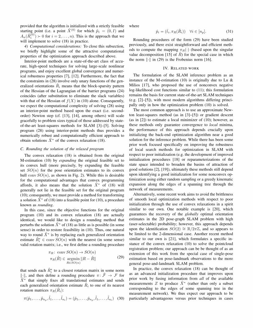
(a) Ground truth (b) Odometric initialization

(c) Levenberg-Marquardt (d) Convex relaxationwith second-stage LMrefinement

Fig. 4. A representative instance of the sphere2500 datasets. (a): Theground truth map. (b): The odometric initialization for this example (objectivefunction value 1.318 E8). (c): The solution obtained by Levenberg-Marquardtusing the odometric initialization (3.420 E7). (d): The solution obtained usingthe two-stage procedure of Section III (7.346 E3); this is the same solutionobtained when initializing Levenberg-Marquardt with the ground truth (a).Note that the objective function values for both (c) and (d) are within ±1%of the median values for the corresponding methods reported in Table II.

relaxation whose solution approximates the optimal solutionof the SLAM problem and can be recovered using a smoothoptimization method initialized at any feasible point. Byprojecting the solution of this relaxation onto the feasible set ofthe original program, we obtain a good estimate of the optimalsolution to the original M-estimation problem, which can itselfbe taken as an initialization for a second-stage local refinementusing the standard least-squares approach. Our approach thusenables the efficient recovery of a high-quality map withoutrequiring high-quality initialization.

ACKNOWLEDGEMENTS

This work was partially supported by a software engineeringinternship at Google, by the Office of Naval Research undergrants N00014-10-1-0936, N00014-11-1-0688 and N00014-13-1-0588, and by NSF Award IIS-1318392, which we grate-fully acknowledge. The authors would also like to thank JulianMason and Kurt Konolige for numerous helpful discussions.

REFERENCES

[1] S. Thrun, W. Burgard, and D. Fox, Probabilistic Robotics. Cambridge,MA: The MIT Press, 2008.

[2] G. Grisetti, D. Rizzini, C. Stachniss, E. Olson, and W. Burgard, “Onlineconstraint network optimization for efficient maximum likelihood maplearning,” in IEEE Intl. Conf. on Robotics and Automation (ICRA),Pasadena, CA, May 2008, pp. 1880–1885.

[3] R. Kummerle, G. Grisetti, H. Strasdat, K. Konolige, and W. Burgard,“g2o: A general framework for graph optimization,” in IEEE Intl. Conf.on Robotics and Automation (ICRA), Shanghai, China, May 2011, pp.3607–3613.

[4] M. Kaess, H. Johannsson, R. Roberts, V. Ila, J. Leonard, and F. Dellaert,“iSAM2: Incremental smoothing and mapping using the Bayes tree,”Intl. J. of Robotics Research, vol. 31, no. 2, pp. 216–235, Feb. 2012.

[5] D. Rosen, M. Kaess, and J. Leonard, “RISE: An incremental trust-regionmethod for robust online sparse least-squares estimation,” IEEE Trans.Robotics, vol. 30, no. 5, pp. 1091–1108, Oct. 2014.

[6] P. Huber, Robust Statistics. Hoboken, N.J.: John Wiley & Sons, 2004.[7] J. Nocedal and S. Wright, Numerical Optimization, 2nd ed. New York:

Springer Science+Business Media, 2006.[8] S. Boyd and L. Vandenberghe, Convex Optimization. Cambridge

University Press, 2004.[9] F. Dellaert and M. Kaess, “Square Root SAM: Simultaneous localization

and mapping via square root information smoothing,” Intl. J. of RoboticsResearch, vol. 25, no. 12, pp. 1181–1203, Dec. 2006.

[10] V. Vandenberghe and Boyd, “Semidefinite programming,” SIAM Review,vol. 38, no. 1, pp. 49–95, Mar. 1996.

[11] J. Saunderson, P. Parrilo, and A. Willsky, “Semidefinite descriptions ofthe convex hull of rotation matrices,” arXiv preprint arXiv:1403.4914,2014.

[12] A. Forsgren, P. E. Gill, and M. H. Wright, “Interior methods fornonlinear optimization,” SIAM Review, vol. 44, no. 4, pp. 525–597, 2002.

[13] R. A. Waltz, J. L. Morales, J. Nocedal, and D. Orban, “An interioralgorithm for nonlinear optimization that combines line search and trustregion steps,” Math. Program., vol. 107, no. 3, pp. 391–408, 2006.

[14] R. H. Byrd, J. Nocedal, and R. A. Waltz, “KNITRO: An integrated pack-age for nonlinear optimization,” in Large-Scale Nonlinear Optimization,G. di Pillo and M. Roma, Eds. Springer, 2006, pp. 35–59.

[15] G. Golub and C. V. Loan, Matrix Computations, 3rd ed. Baltimore,MD: Johns Hopkins University Press, 1996.

[16] S. Umeyama, “Least-squares estimation of transformation parametersbetween two point patterns,” IEEE Trans. Pattern Analysis and MachineIntelligence, vol. 13, no. 4, pp. 376–380, 1991.

[17] F. Lu and E. Milios, “Globally consistent range scan alignment forenvironmental mapping,” Autonomous Robots, vol. 4, pp. 333–349, Apr.1997.

[18] M. Pfingsthorn and A. Birk, “Simultaneous localization and mappingwith multimodal probability distributions,” Intl. J. of Robotics Research,vol. 32, no. 2, pp. 143–171, 2013.

[19] E. Olson, J. Leonard, and S. Teller, “Fast iterative alignment of posegraphs with poor initial estimates,” in IEEE Intl. Conf. on Robotics andAutomation (ICRA), Orlando, FL, May 2006, pp. 2262–2269.

[20] L. Carlone and A. Censi, “From angular manifolds to the integerlattice: Guaranteed orientation estimation with application to pose graphoptimization,” IEEE Trans. Robotics, vol. 30, no. 2, pp. 475–492, Apr.2014.

[21] M. Horowitz, N. Matni, and J. Burdick, “Convex relaxations of SE(2)and SE(3) for visual pose estimation,” in IEEE Intl. Conf. on Roboticsand Automation (ICRA), Hong Kong, China, Jun. 2014.