1

ABSTRACT

The development of energy-conscious embedded and/or mobile sys-tems exposes a trade-off between energy consumption and systemperformance. Recent microprocessors have incorporated dynamicvoltage scaling as a tool that system software can use to explore thistrade-off. Developing appropriate heuristics to control this feature isa non-trivial venture; as has been shown in the past, voltage-scalingheuristics that closely track perceived performance requirements donot save much energy, while those that save the most energy tend todo so at the expense of performance—resulting in poor responsetime, for example. We note that the task of dynamically scaling pro-cessor speed and voltage to meet changing performance require-ments resembles a classical control-systems problem, and so weapply a bit of control theory to the task in order to define a new volt-age-scaling algorithm. We find that, using our nqPID (not quite PID)algorithm, one can improve upon the current best-of-class heuris-tic—Pering’s AVG

N

algorithm, based on Govil’sAGED_AVERAGES algorithm and Weiser’s PAST algorithm—inboth energy consumption and performance. The study is execution-based, not trace-based; the voltage-scaling heuristics were integratedinto an embedded operating system running on a Motorola M-CORE processor model. The applications studied are all members ofthe MediaBench benchmark suite.

Categories and Subject Descriptors

C.3[Special-purpose and Application-based systems]Real-time andEmbedded Systems.

General Terms

Algorithms, Performance, Design.

Keywords

Low-power, dynamic voltage scaling, PID, nqPID.

1. INTRODUCTION

Battery life (i.e. energy supply and rate of depletion) and execution-time performance are arguably the two chief parameters determiningthe usability of mobile embedded devices such as PDAs, cellphones,wearables, and handheld/notebook computers. The problem is thatthe goals of high performance and low energy consumption are atodds with each other: while successive generations of general-pur-pose microprocessors have realized improved performance levels,they have also become more power-hungry. Users demand higherperformance without an accompanying cost in battery life or heatdissipation, but it is not always possible to deliver this. Until Intel’srecent emphasis on low power, many mobile computers used less-than-cutting-edge processors because the longer battery life andlower heat dissipation of those processors made them more attractivein mobile environments despite their lower performance levels—forexample, P3 notebooks when P4 was the norm for desktops, orhandhelds that were MIPS-based rather than Pentium-based.

The demand for extracting good performance while having lowenergy consumption has caused processor manufacturers to take acloser look at power-management strategies. More and more chipssupporting dynamic power-management are rolling out everyday,with one of the more popular mechanisms being dynamic voltage-frequency scaling (called simply “dynamic voltage scaling” or DVS[9]), in which the processor’s clock frequency and supply voltagecan be changed in tandem by software during the course of opera-tion.

Using such a mechanism, a processor can be set to use the mostappropriate performance level at any given moment, spreadingbursty traffic out over time and avoiding hurry-up-and-wait scenar-ios that consume more energy than is truly required for the computa-tion at hand (see Figure 1). As Weiser points out, idle time representswasted energy, even if the CPU is stopped [16].

Voltage and frequency are scaled together to achieve reductions inenergy per computation. Scaling frequency alone is insufficientbecause, while reducing the clock frequency does reduce a proces-sor’s power consumption, a computation’s execution time is to a firstapproximation linearly dependent on clock frequency, and the clock-speed reduction can result in the computation taking more time butusing the same total energy. Because power consumption is quadrat-ically dependent on voltage level, scaling the voltage level propor-tionally along with the clock frequency offers a significant totalenergy reduction while running a processor at a reduced perfor-mance level. Transmeta’s Crusoe, AMD’s K-6, and Intel’s XScale(née Digital StrongARM) and Pentium III & IV are all examples of

A Control-Theoretic Approach to Dynamic Voltage Scheduling

Ankush Varma, Brinda Ganesh, Mainak Sen, Suchismita Roy Choudhury, Lakshmi Srinivasan, and Bruce Jacob

Dept. of Electrical & Computer Engineering University of Maryland at College Park

College Park, MD 20742http://www.ece.umd.edu/~blj/embedded/

{ankush,blj}@eng.umd.edu

Permission to make digital or hard copies of all or part of this work forpersonal or classroom use is granted without fee provided that copies are notmade or distributed for profit or commercial advantage and that copies bearthis notice and the full citation on the first page. To copy otherwise, orrepublish, to post on servers or to redistribute to lists, requires prior specificpermission and/or a fee.Appears in Proc. International Conference on Compilers, Architectures, and Synthesis for Embedded Systems (CASES 2003), October 30 – November 1, 2003, San Jose CA, USA.Copyright © 2003 ACM 1-58113-399-5/01/0011...$5.00.

2

advanced high-performance microprocessors that support dynamicvoltage scaling for power management.

However, it is not sufficient to merely have a chip that

supports

voltage scaling. There must exist an entity, whether hardware orsoftware, that decides when to scale the voltage and by how much toscale it. This decision is essentially a prediction of the near-futurecomputational needs of the system and is generally made on thebasis of the recent computing requirements of all tasks and threadsrunning at the time. The sole entity that has access to all of this glo-bal information (resource usage, demand, and availability) is theoperating system [7], because all tasks are visible to it even if thesystem design makes them invisible to each other. Thus, in actualimplementations, the decision to change the processor speed andvoltage level is typically made by the OS.

The goal of a voltage-scaling heuristic is to adapt the processor’sperformance level to match the expected performance requirements.The development of good heuristics is a tricky problem, as pointedout by Weiser et al. [16]: heuristics that closely track performancerequirements save little energy, while those that save the mostenergy tend to do so at the expense of performance—resulting inpoor response time, for example.

Recent studies [16, 6, 9, 10, 7, 12] investigate numerous differentheuristics that estimate near-future computational load and set theprocessor’s speed and voltage level accordingly. Nearly all of thealgorithms studied represent different trade-offs in assigning weightsto recent observed processing requirements. The only dynamic vari-ability in the assignment of weights has been through recognizingand exploiting patterns in the performance requirements. For exam-ple, a system could predict its future needs from an average of themost recently observed needs unless the recent requirements match

some pattern of behavior observed in the distant past, in which casethe prediction is based on the distant past behavior instead of theaverage of recent behavior. However, such schemes have been foundto perform no better than static weighted averages [6].

To our knowledge, no published heuristic has incorporated the

rate of change

in a system’s processing requirements—the rate ofchange, the derivative, is a powerful tool at the heart of control-sys-tems theory [3] and well worth exploring in the context of dynamicvoltage scaling, as it indicates the rapidity with which a heuristicought to respond to changes in a system’s processing requirements.Without considering the derivative, any heuristic using a fixedassignment of weights will always respond to changes in computingrequirements at the same rate. When a relatively idle system is pre-sented with a burst of activity, such a heuristic will take too long tobring the speed of the processor up to the appropriate level, resultingin a window of time during which the energy consumption is low butthe system’s performance is poor.

This paper presents a heuristic for dynamic voltage scaling thatincorporates the rate of change in the recent processing require-ments. We took the equation describing a PID controller (

Propor-tional-Integral-Derivative

), a classical control-systems algorithm [3,8, 17] as our starting point, and modified it to suit the application athand

-

dynamic voltage scaling. We used this new nqPID (not quitePID) algorithm and executed a full system (applications plus embed-ded OS with the nqPID controller integrated into the OS) running on

SimBed

, an embedded-systems simulation testbed that accuratelymodels the performance and energy consumption of an embeddedmicroprocessor, complete with I/O and timing interrupts, system-level support, and the ability to run the same unmodified binariesthat execute on our hardware reference platforms [2].

Figure 1: Energy consumption vs. power consumption. Not every task needs the CPU’s full computational power. In many cases, for example theprocessing of video and audio streams, the only performance requirement is that the task meet a deadline, see Fig. (a). Such cases create opportunities to runthe CPU at a lower performance level and achieve the same perceived performance while consuming less energy. As Fig. (b) shows, reducing the clockfrequency of a processor reduces power consumption but simply spreads a computation out over time, thereby consuming the same total energy as before. AsFig. (c) shows, reducing the voltage level as well as the clock frequency achieves the desired goal of reduced energy consumption and appropriate performancelevel.

Power V2F∝

Power V2F

2---∝

PowerV2----

2F2---∝

Time

Time

Time

Energy E

Energy E

Energy E/4

Task ready at time 0;

(a)

(b)

(c)

no other task is ready.Task requires time T to complete, assuming top clock frequency F.

Task s outputis not neededuntil time 2T

Reducing the clock frequency F by halflowers the processor s power consumptionand still allows task to complete by deadline.

The energy consumption remains the same.

Reducing the voltage level V by half reduces the power level further, without anycorresponding increase in execution time.

3

Most studies of dynamic voltage scaling have been trace-based,with Grunwald et al. [7] providing one of the few execution-basedstudies. We have implemented the most efficient of the publishedheuristics, as determined by Grunwald (Pering’s AVG

N

algorithm[9], based on Govil’s AGED_AVERAGES algorithm [6] andWeiser’s PAST algorithm [16]), and compared its performance andenergy behavior with our scheme. We find that the nqPID schemereduces CPU energy of an embedded system between 70 and 80%

1

(an improvement over AVG

N

of 10–50%), while maintaining real-time behavior: specifically, the jitter in task execution time is limitedto roughly 2% (an improvement over AVG

N

of a factor of two).An interesting point is that the algorithm’s effectiveness is not

obtained through careful tuning of parameters; our results are for aset of controller parameters that were chosen to be conservative.Fine-tuning of the parameters can yield jitter improvements of a fac-tor of two and further energy reductions of 30%.

A sensitivity analysis shows that neither system performance norenergy consumption is particularly sensitive to the nqPID control-ler’s parameters. The jitter values are under 4% of the desired periodfor all parameter configurations, and more than half of the configura-tions yield jitter less than 1%. The energy consumption results varyby roughly a factor of two from worst configuration to best: Theenergy consumed by systems with different nqPID configurationsranges from 17% to 39% of the energy consumed by a system with-out dynamic voltage scaling. More than half of the configurationsyield energy results within 25% of the optimum. We conclude fromthis experiment that classical control-systems theory is very applica-ble to dynamic voltage scaling, and we intend to explore the synergyfurther.

2. BACKGROUND

This section presents brief backgrounds on dynamic voltage scaling,voltage scheduling algorithms, related work, and the structure andbehavior of classical PID control algorithms.

2.1. Energy Reduction in CMOS

The instantaneous power consumption of CMOS devices, such asmicroprocessors, is measured in Watts (W) and, to a first approxima-tion, is directly proportional to V

2

F:

where V is the voltage supply and F is the clock frequency. Theenergy consumed by a computation that requires T seconds is mea-sured in Joules (J) and is equal to the integral of the instantaneouspower over time T. If the power consumption remains constant overT, the resultant energy drain is simply the product of power and time.

It is possible to save energy by reducing V, F, or both. In practice,V is not scaled by itself. For high-speed digital CMOS, the maxi-mum clock frequency is limited by the following relation [1]:

where V

THN

is the threshold voltage. The threshold voltage must belarge enough to overcome noise in the circuit, so the right hand sidein practice ends up being a constant proportion of V, for given tech-nology characteristics. Usually microprocessors operate at the low-

est voltage level that will support the desired clock frequency, sothere is not much headroom to lower the voltage level by itself.

The term

voltage scaling

refers to changing the voltage and thefrequency together, typically in proportional amounts. The term

volt-age scheduling

refers to operating-system scheduling policies thatuse a processor’s voltage scaling facility to achieve higher levels ofenergy efficiency. For example, it is more efficient to run a processorat a continuous lower speed than to run it at full speed until the taskis completed and then idling, as is illustrated in Figure 1.

2.2. Clock/Voltage Scheduling Algorithms

Voltage scheduling can be separated into two tasks [6]:

•

Load Prediction

: predicting the future system load based on past behavior.

•

Speed-Setting

: Using the load prediction to set the voltage level and clock frequency.

The schedulers we have implemented are

interval schedulers

[16].They perform the load prediction and speed-setting tasks at regularintervals as the system runs. Interval schedulers use the global sys-tem state to calculate how busy the system is and typically do notuse knowledge of individual task threads.

The primary trade-off is between energy and performance. Weiserobserved that a system attempting to run at a flat optimal speed willhave significant energy savings, but it will do so at the cost of miss-ing deadlines. On the other hand, a system that responds quickly tochanges in the workload will not be as energy-optimal [16].

In the choice of algorithm, this becomes a choice between

smoothing

and

prediction

[6]. A policy that tries to smooth outchanges in speed will reduce energy cost, while one that does accu-rate prediction will improve performance. In theory, it should bepossible to achieve both goals to a reasonable degree.

2.3. Related Work

Weiser’s seminal 1994 paper on voltage scheduling [16] describedthe PAST algorithm, along with two other ideal (unimplementable)algorithms. The PAST heuristic predicts that the current interval willbe as busy as the immediately preceding interval. To date, it is stillone of the best-performing algorithms, as shown by Grunwald [7].

Simulation-based and execution-based analysis of various voltagescaling strategies has been done for workstations [6, 16, 5] and,more recently, low-power embedded devices [12] and PDAs [7, 10].Govil et al. study a wide range of heuristics from weighted averagesof past behavior to pattern matching of processor utilization [6]. Per-ing et al. look at another range of heuristics and use a “clipped-delay” metric (inspired by Endo et al. [4]) to quantify the resilienceof an application to slight degradations in performance [9]. Whereasother studies have used processor idle time as the primary means ofpredicting future performance requirements, Flautner et al. proposea heuristic that observes inter-process communication patterns toidentify scenarios in which the OS can delay tasks until their resultsare used by another process [5].

Most studies have been trace-driven and/or have considered ideal,oracle-based heuristics to ascertain the optimal energy-performancetrade-off. Execution-driven studies, in which a real operating systemis instrumented with realizable heuristics, include those by Pering[11], Grunwald [7], and Pillai [12]. Pering investigates designoptions for extremely low-power general-purpose microprocessors;Grunwald implements the best-of-class voltage-scheduling heuris-tics in a Linux-based PDA environment; and Pillai simulates anextensive range of parameters, then implements heuristics using achosen parameter set on an AMD K6-2-based laptop.

1. The resultant energy consumption of the dynamic voltage scaled system is 20–30% of the energy consumed by a system without dynamic volt-age scaling.

P V2F∝

FMAX

V V THN–( )V

----------------------------2

∝

4

As far as heuristics go, the cutting edge so far seems to be Per-ing’s AVG

N

algorithm, as demonstrated by Grunwald comparing anumber of different algorithms on the Itsy handheld computer [7].AVG

N

is a subset and simplification of Govil’s AGED_AVERAGESalgorithm and reminiscent of Weiser’s PAST algorithm. UnderAVG

N

, an exponential moving average with decay N of the previousintervals is used. That is, at each interval, it computes a “weightedutilization” at time t,

which is a function of the utilization of the previous interval U[t].The AGED_AVERAGES algorithm allows any geometricallydecaying factor, not just N/N+1.

Grunwald’s findings indicate that AVG

N

cannot settle on a clockspeed that maximizes CPU utilization. The set of parameters chosencould result in optimal performance for a single application, butthese tuned parameters need not work for other applications. How-ever, they found that the AVG

N

policy resulted in both the mostresponsive system behavior and the most significant energy reduc-tion of all the policies they examined.

2.4. PID Control

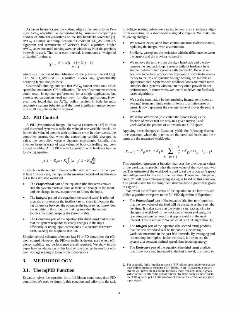
A PID (Proportional-Integral-Derivative) controller [17] is oftenused in control systems to make the value of one variable “track”, orfollow, the value of another with minimum error. In other words, thecontroller ensures that when the controlling variable changes itsvalue, the controlled variable changes accordingly. Usually, thisinvolves keeping track of past values of both controlling and con-trolled variables. A full PID control algorithm with feedback has thefollowing equation:

in which

y

is the output of the controller at time

t ,

and

x

is the inputat time

t

. In our case, the input is the measured workload and the out-put is the estimated workload.

•

The

Proportional

part of the equation (the first term) makes sure the system reacts as soon as there is a change in the input, and the change in new output tries to follow the input.

•

The

Integral

part of the equation (the second term) is referred to as the error term or the feedback term, since it measures the net difference between the output an the input so far. It provides the stability in the circuit by making sure that the output follows the input, keeping the system stable.

•

The

Derivative

part of the equation (the third term) makes sure that the system responds to steady changes in the input efficiently. A rising input corresponds to a positive derivative term, causing the output to rise too.

Simpler control schemes often use just PI or PD controllers for effi-cient control. However, the PID controller is the one used where effi-ciency, stability and performance are all required. We show in thispaper how an adaptation of this kind of function can be used for effi-cient voltage scaling in today’s microprocessors.

3. METHODOLOGY

3.1. The nqPID Function

Equation gives the equation for a full-blown continuous-time PIDcontroller. We need to simplify this equation and tailor it to the task

of voltage scaling before we can implement it as a software algo-rithm executing on a discrete-time digital computer. We make thefollowing changes:

•

We convert the equation from continuous-time to discrete-time, replacing the integral with a summation.

•

Similarly, we replace the derivative with the difference between the current and the previous value of

x

.

•

We remove the term

y

from the right hand side and thereby remove the feedback loop. Systems without feedback have simpler behavior than systems with feedback

2

. Because our goal was to perform a first-order exploration of control-systems theory to the task of dynamic voltage scaling, we felt this an appropriate step. Systems with feedback loops are much more complex than systems without, but they often provide better performance. In future work, we intend to delve into feedback-based algorithms.

•

We cut the summation in the remaining integral term (now an average) from an infinite series of terms to a finite series of terms. It now represents the average value of

x

over the past

m

intervals.

•

We define

utilization

(also called the

system load

) as the fraction of cycles that are busy in a given interval, and

workload

as the product of utilization and CPU speed.

Applying these changes to Equation yields the following discrete-time equation, where the

y

terms are the predicted loads and the

x

terms are the measured workloads:

This equation represents a function that uses the previous

m

valuesof the workload to predict what the next value of the workload willbe. This estimate of the workload is used to set the processor’s speedand voltage level for the next time quantum. Throughout this paper,“nqPID” will refer voltage-scaling strategies based on this equation.The pseudo-code for the simplified, discrete-time algorithm is givenin Figure 2.

We revisit the different terms of the equation to see how this sim-plified algorithm compares to the full PID algorithm of Equation :

•

The

Proportional

part of the equation (the first term) predicts that the next value of the load will be the same as that seen the last time. It makes sure that the system can react quickly to changes in workload. If the workload changes suddenly, the operating system can react to it appropriately in the next interval. This is similar to Weiser et. al.’s PAST algorithm [16].

•

The

Integral

part of the equation (the second term) predicts that the next workload will be the same as the average workload measured in the past few intervals. By averaging and “smoothing the ripples” in the workload, it tries to run the system at a constant optimal speed, thus reducing energy.

•

The

Derivative

part of the equation (the third term) predicts that if the workload increased in the last interval, it is likely to

t[ ] N W t 1–[ ]× U t 1–[ ]+N 1+

-----------------------------------------------------------=

y t( ) KPx KI x y–( ) td0

t

∫ KDdxdt------+ +=

2. For example, finite impulse response (FIR) filters are simpler to analyze than infinite impulse response (IIR) filters. In an IIR system, a pulse’s effects will never die due to the feedback loop; transient input signals will continue to affect the output forever. To make analysis more tracta-ble, FIR systems put a finite window of time on the effects of any given input signal.

yn 1+ KP xn KI

xim---

n m– 1+

n

∑×+× KD xn xn 1––( )×+=

5

increase again and at the same rate. This is the real predictive part of the equation, because it anticipates the changes that might occur in the workload and lets the operating system make a better choice of the required speed setting.

By themselves, these are not very efficient. For example, the propor-tional part does not adequately study past behavior, and so cannotoptimize power requirements. The integral part optimizes energy atthe cost of performance by not reacting fast enough (as it is an aver-age of n values). The derivative part by itself cannot predict theactual workload, only changes in the workload, so it is unsuitable forsteady-state operation. However, the consensus of all of these canprovide a very good estimate of what the next value of the workloadis likely to be. We take all three effects into account by taking aweighted sum of them.

There are several different but equivalent ways of looking at thenqPID equation:

• From the mathematical point of view, this is a function that extrapolates the value of a given variable based on its previous values.

• From the control-systems point of view, this kind of transfer function provides fast response times and low errors.

• From the computer engineering point of view, this is just a data value prediction algorithm that is predicting the value of the system load based on its previous behavior.

Another advantage of this type of control is that it is relatively insen-sitive to changes in its parameters: it provides good response for anentire range, rather than a few values, of the coefficients. In otherwords, the same coefficients could be used across all applications,while still giving good performance. This is quantified later in oursensitivity analysis.

3.2. System Issues

For this project, Motorola’s 32-bit M-CORE architecture [14, 13,15] was used as the model architecture for our emulator. This archi-tecture was chosen because it is one of the cutting edge embedded

processors on the market today, and the M-CORE was designed forhigh performance and very low power operation. The M-COREallows 36 voltage scaling levels, corresponding to clock frequenciesfrom 2 to 20MHz.

As the target operating system, we used NOS [2], a bare-bonesmulti-rate task scheduler reminiscent of typical “roll-your-own”RTOSs found in many commercial embedded systems. We mademodifications to the NOS kernel that enable us to choose between asystem with no voltage scaling, an nqPID algorithm (with m=10,Kp=0.4, Ki=0.2, Kd=0.4) and the AVGN algorithm (with N=3 [9,10, 7]). The nqPID coefficients were chosen to reflect a middle-of-the-road configuration that would not be fine-tuned to any particularbenchmark (cf. Figure 6). At any rate, as the figure shows, thenqPID controller is only weakly sensitive to changes in moderatevalues of these parameters.

Care was taken to implement the Grunwald implementation faith-fully. All parameters other than the algorithms themselves were keptthe same to ensure a fair algorithm-to-algorithm comparison. TheAVG algorithm was set to change speed whenever the workloaddrifted out of its optimum range of 50-70% [7].

For benchmarks we used several benchmarks from the Media-Bench suite [18]. To assess the effects of an increasing workload,readings were taken with different numbers of tasks running simul-taneously (2, 4, and 8), and with tasks having different periods.More than eight tasks could not be run together without completelymissing deadlines, and in nearly all cases even 8 tasks represents aworkload level at which most deadlines are missed.

Lastly, note that a microprocessor cannot process data while itscore voltage or operating frequency is changing. It takes a finiteamount of time, and a finite amount of energy, to effect this change.Changing voltage levels and clock frequencies lowers performanceand has a “cost” in terms of energy that must be made up by theenergy it saves. We use the same time values presented by Grun-wald: clock scaling takes 200 microseconds; voltage scaling takes250 microseconds. The energy consumed during the transition ismodelled as if the processor is executing the most energy-intensiveinstructions.

Figure 2: Psuedo-code for the nqPID algorithm. The code shows only the speed-setting portion of the algorithm; as a result of the calculations, the CPU’sspeed is set to be directly proportional to the estimated load. Not shown is the update of the load[] array, any error-checking, etc.

// window of previous N actual system loadsload_t load[WINDOW_SIZE];

// Proportional termestimated_load = Kp * load[0];

// Integral termfor (i=0;, tmp=0; i<WINDOW_SIZE; i++) {

tmp += load[i] / WINDOW_SIZE;}estimated_load += Ki * tmp;

// Derivative termestimated_load += Kd * (load[0] - load[1]);

// Speed SettingsetPercentSpeed = estimated_load / MAX_LOAD;

The proportional term attempts to keep upwith changes in the measured system load.

The integral term attempts to average out noise in the system load and thereby avoid switching clock speeds and voltage levels unnecessarily for example, aswould happen in response to a brief spikeof processor activity during an otherwise idle period.

The derivative term attempts to identifyrapid changes in system load so as to keepup when the system suddenly needs high levels of performance, but also to quickly scale performance levels down when the system becomes idle.

6

4. RESULTS

We present a comparison of the two heuristics in terms of how wellthey trade-off energy and performance; we present a sensitivity anal-ysis; and we discuss how the run-time behavior of the algorithmsaffects their efficiency.

4.1. Energy and Performance

Our experiments use programs from the MediaBench suite ofembedded-systems applications [18] that we have ported to the NOSembedded operating system. To vary the load on the system, two dif-

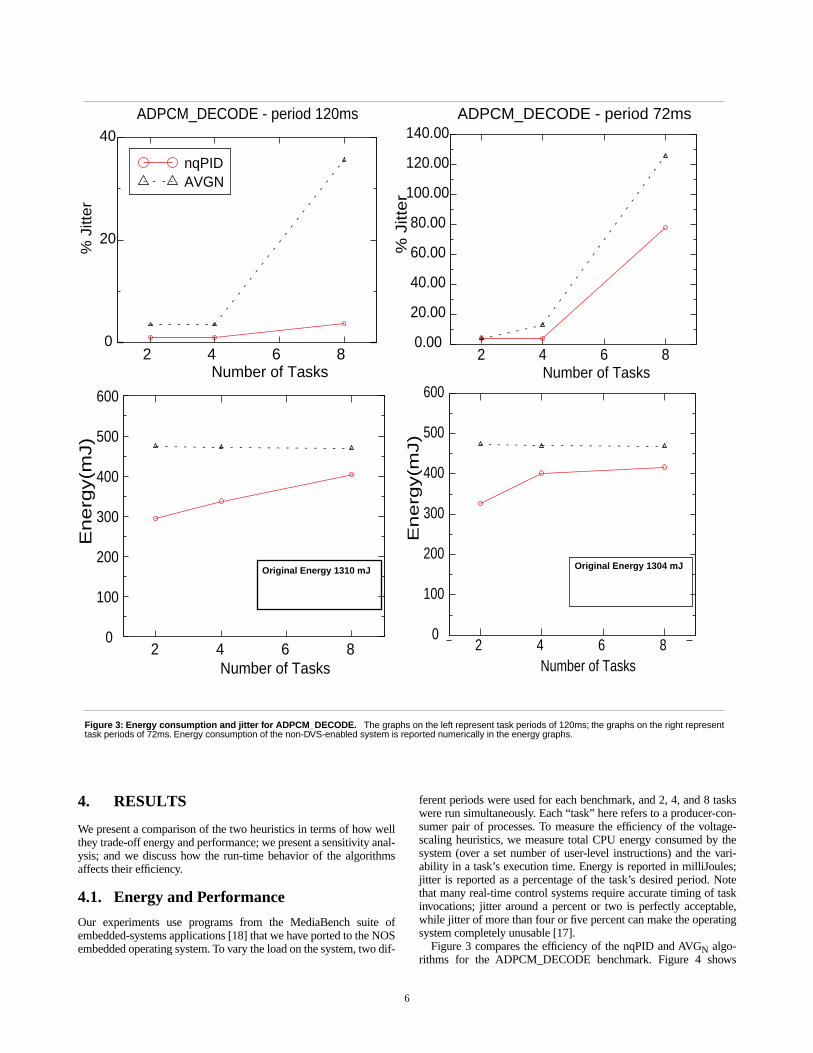
ferent periods were used for each benchmark, and 2, 4, and 8 taskswere run simultaneously. Each “task” here refers to a producer-con-sumer pair of processes. To measure the efficiency of the voltage-scaling heuristics, we measure total CPU energy consumed by thesystem (over a set number of user-level instructions) and the vari-ability in a task’s execution time. Energy is reported in milliJoules;jitter is reported as a percentage of the task’s desired period. Notethat many real-time control systems require accurate timing of taskinvocations; jitter around a percent or two is perfectly acceptable,while jitter of more than four or five percent can make the operatingsystem completely unusable [17].

Figure 3 compares the efficiency of the nqPID and AVGN algo-rithms for the ADPCM_DECODE benchmark. Figure 4 shows

Figure 3: Energy consumption and jitter for ADPCM_DECODE. The graphs on the left represent task periods of 120ms; the graphs on the right representtask periods of 72ms. Energy consumption of the non-DVS-enabled system is reported numerically in the energy graphs.

2 4 6 8Number of Tasks

0

20

40

% J

itter

nqPIDAVGN

ADPCM_DECODE - period 120ms

2 4 6 8Number of Tasks

0.00

20.00

40.00

60.00

80.00

100.00

120.00

140.00

% J

itter

ADPCM_DECODE - period 72ms

2 4 6 8Number of Tasks

0

100

200

300

400

500

600

En

erg

y(m

J)

2 4 6 8Number of Tasks

0

100

200

300

400

500

600E

ne

rgy(m

J)

Original Energy 1310 mJ Original Energy 1304 mJ

7

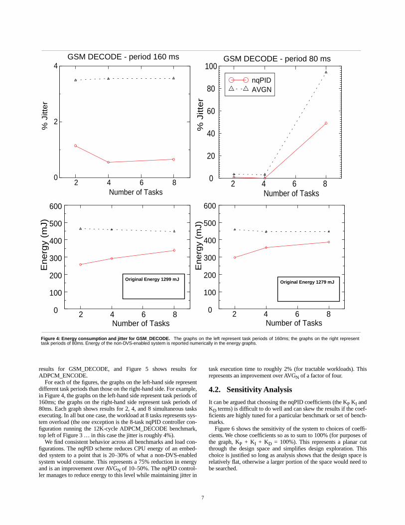
results for GSM_DECODE, and Figure 5 shows results forADPCM_ENCODE.

For each of the figures, the graphs on the left-hand side representdifferent task periods than those on the right-hand side. For example,in Figure 4, the graphs on the left-hand side represent task periods of160ms; the graphs on the right-hand side represent task periods of80ms. Each graph shows results for 2, 4, and 8 simultaneous tasksexecuting. In all but one case, the workload at 8 tasks represents sys-tem overload (the one exception is the 8-task nqPID controller con-figuration running the 12K-cycle ADPCM_DECODE benchmark,top left of Figure 3 … in this case the jitter is roughly 4%).

We find consistent behavior across all benchmarks and load con-figurations. The nqPID scheme reduces CPU energy of an embed-ded system to a point that is 20–30% of what a non-DVS-enabledsystem would consume. This represents a 75% reduction in energyand is an improvement over AVGN of 10–50%. The nqPID control-ler manages to reduce energy to this level while maintaining jitter in

task execution time to roughly 2% (for tractable workloads). Thisrepresents an improvement over AVGN of a factor of four.

4.2. Sensitivity Analysis

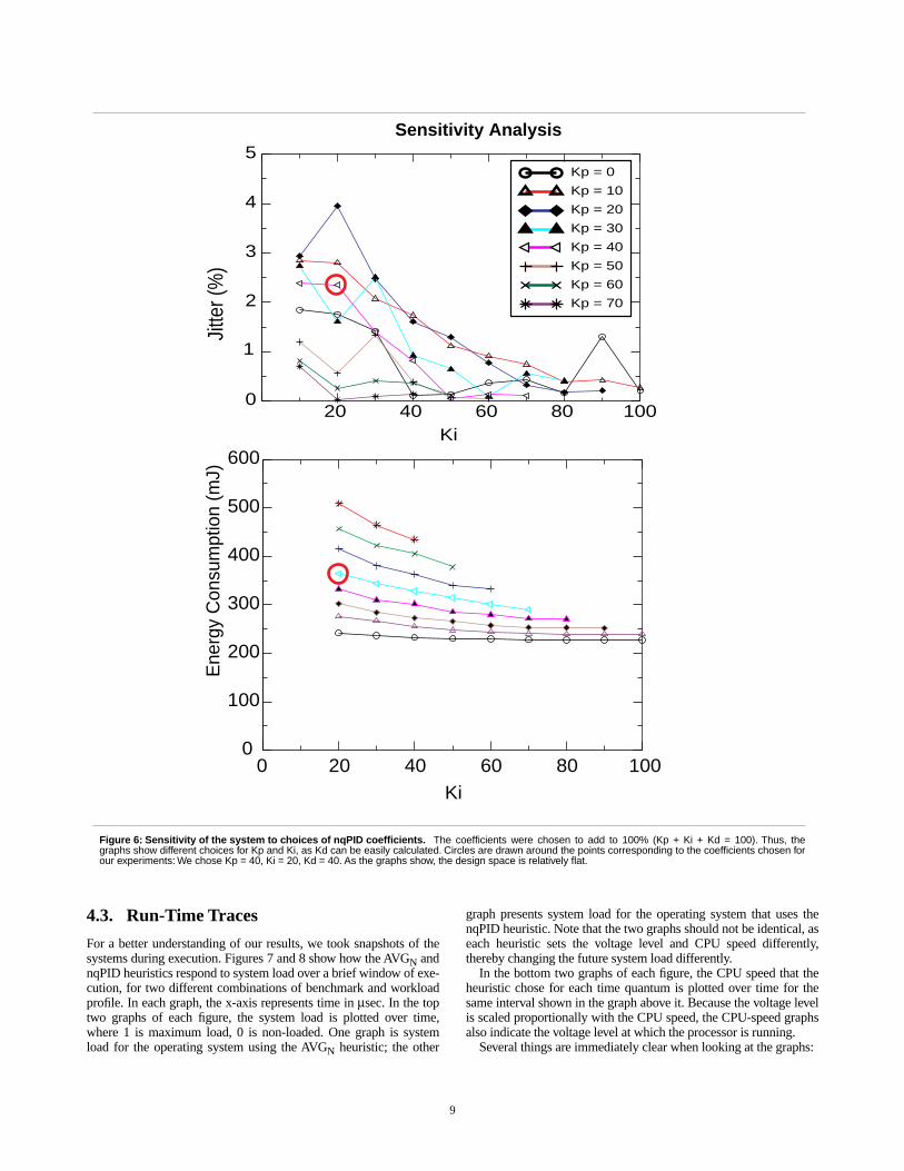
It can be argued that choosing the nqPID coefficients (the KP KI andKD terms) is difficult to do well and can skew the results if the coef-ficients are highly tuned for a particular benchmark or set of bench-marks.

Figure 6 shows the sensitivity of the system to choices of coeffi-cients. We chose coefficients so as to sum to 100% (for purposes ofthe graph, KP + KI + KD = 100%). This represents a planar cutthrough the design space and simplifies design exploration. Thischoice is justified so long as analysis shows that the design space isrelatively flat, otherwise a larger portion of the space would need tobe searched.

Figure 4: Energy consumption and jitter for GSM_DECODE. The graphs on the left represent task periods of 160ms; the graphs on the right representtask periods of 80ms. Energy of the non-DVS-enabled system is reported numerically in the energy graphs.

2 4 6 8Number of Tasks

0

2

4

% J

itte

r

GSM DECODE - period 160 ms

2 4 6 8Number of Tasks

0

100

200

300

400

500

600

En

erg

y (m

J)

2 4 6 8Number of Tasks

0

20

40

60

80

100

% J

itte

r

GSM DECODE - period 80 ms

2 4 6 8Number of Tasks

0

100

200

300

400

500

600E

ne

rgy

(mJ)

nqPIDAVGN

Original Energy 1299 mJOriginal Energy 1279 mJ

8

Note that the graphs only show different values for KP and KI;because we are searching a planar section of the space (not all com-binations of Kj are valid), KD need not be shown as it can be easilycalculated. In the figures, circles are drawn around the points corre-sponding to the coefficients chosen for our experiments: As men-tioned earlier, we chose KP = 40%, KI = 20%, and KD = 40%.

The graphs represent the averages over all configurations of allbenchmarks—except for 8-task configurations which in most casesrepresent intractable workloads.

As the graphs show, the design space is relatively flat, and most ofthe designs lie within 25% of the optimal configuration. For exam-ple, in the Energy graph, more than half of the designs lie below the300mJ mark. In the Jitter graph, we see that the design space is a bitmore chaotic, but two-thirds of the designs lie below 1.5% jitter, andno design exceeds 4%. Moreover, there is a large region of the

design space, corresponding to values of KI between 40 and 80inclusive, that has very flat behavior and excellent jitter values, mostunder 1%.

Why did we not choose one of these optimal points to begin with,for purposes of comparison? Why did we choose the proportion 40-20-40 for our coefficients? It is often found that coefficients chosenfor voltage-scaling studies are extremely benchmark-specific. A par-ticular set of coefficients may run extremely well for a particularbenchmark and completely fail to deliver for others. Also, even thevalues of the coefficients for a particular application cannot beknown on an a priori basis. We felt that to present the algorithm inthe most appropriate light, we must not tailor our parameters to theapplications we run, so that our results would indicate how thedesign would likely fare in a typical real-world implementation.Thus, the proportions chosen are conservative.

Figure 5: Energy consumption and jitter for ADPCM_ENCODE. The graphs on the left represent task periods of 160ms; the graphs on the right representtask periods of 80ms. Energy of the non-DVS-enabled system is reported numerically in the energy graphs.

2 4 6 8Number of Tasks

0

20

40

% J

itte

r

ADPCM ENCODE - period 160 ms

2 4 6 8Number of Tasks

0

100

200

300

400

500

600

Energ

y (m

J)

Original Energy 1310 mJ

nqPIDAVGN

2 4 6 8Number of Tasks

0

50

100

150

200

% J

itte

r

ADPCM ENCODE - period 80 ms

2 4 6 8Number of Tasks

0

100

200

300

400

500

600E

ne

rgy

(mJ)

Original Energy 1300 mJ

9

4.3. Run-Time Traces

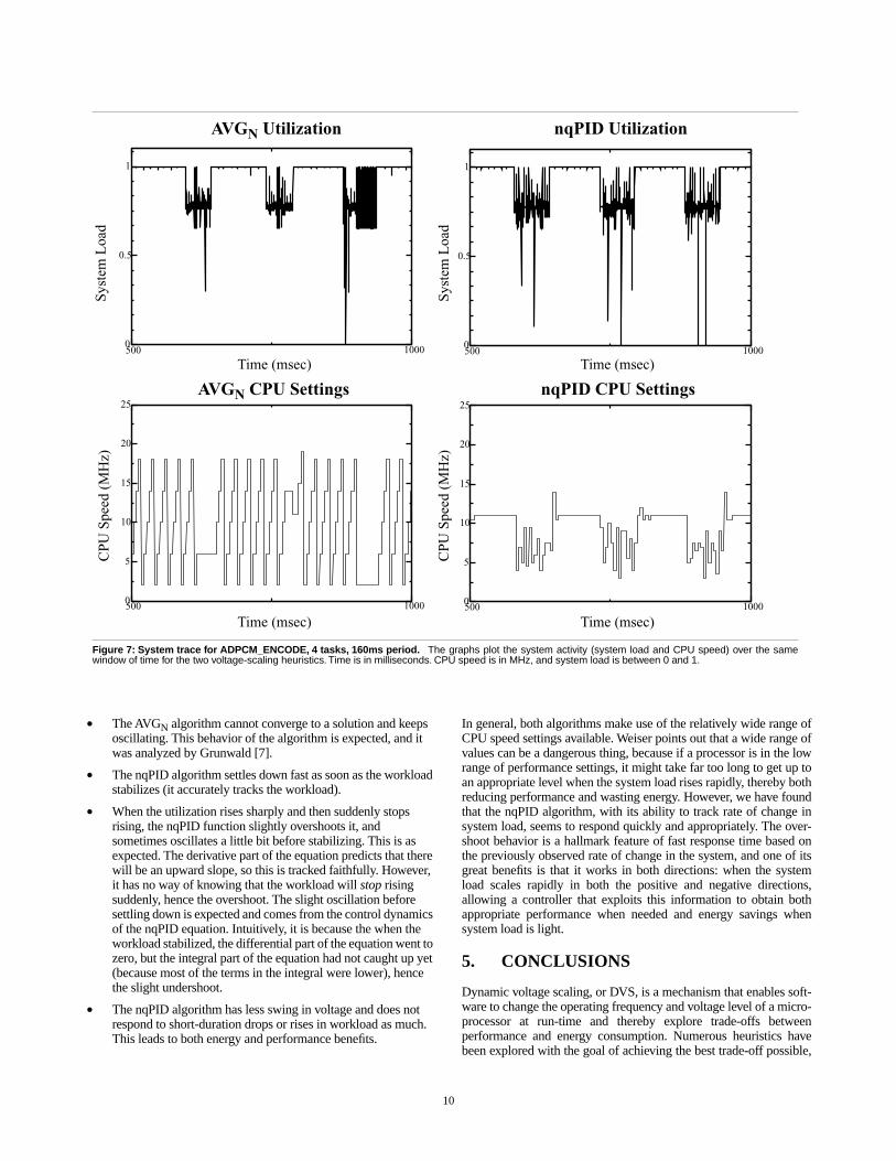
For a better understanding of our results, we took snapshots of thesystems during execution. Figures 7 and 8 show how the AVGN andnqPID heuristics respond to system load over a brief window of exe-cution, for two different combinations of benchmark and workloadprofile. In each graph, the x-axis represents time in µsec. In the toptwo graphs of each figure, the system load is plotted over time,where 1 is maximum load, 0 is non-loaded. One graph is systemload for the operating system using the AVGN heuristic; the other

graph presents system load for the operating system that uses thenqPID heuristic. Note that the two graphs should not be identical, aseach heuristic sets the voltage level and CPU speed differently,thereby changing the future system load differently.

In the bottom two graphs of each figure, the CPU speed that theheuristic chose for each time quantum is plotted over time for thesame interval shown in the graph above it. Because the voltage levelis scaled proportionally with the CPU speed, the CPU-speed graphsalso indicate the voltage level at which the processor is running.

Several things are immediately clear when looking at the graphs:

Figure 6: Sensitivity of the system to choices of nqPID coefficients. The coefficients were chosen to add to 100% (Kp + Ki + Kd = 100). Thus, thegraphs show different choices for Kp and Ki, as Kd can be easily calculated. Circles are drawn around the points corresponding to the coefficients chosen forour experiments: We chose Kp = 40, Ki = 20, Kd = 40. As the graphs show, the design space is relatively flat.

Sensitivity Analysis

20 40 60 80 100Ki

0

1

2

3

4

5

Jitte

r (%

)

0 20 40 60 80 100Ki

0

100

200

300

400

500

600

Ene

rgy

Con

sum

ptio

n (m

J)

Kp = 0

Kp = 10

Kp = 20

Kp = 30

Kp = 40

Kp = 50

Kp = 60

Kp = 70

10

• The AVGN algorithm cannot converge to a solution and keeps oscillating. This behavior of the algorithm is expected, and it was analyzed by Grunwald [7].

• The nqPID algorithm settles down fast as soon as the workload stabilizes (it accurately tracks the workload).

• When the utilization rises sharply and then suddenly stops rising, the nqPID function slightly overshoots it, and sometimes oscillates a little bit before stabilizing. This is as expected. The derivative part of the equation predicts that there will be an upward slope, so this is tracked faithfully. However, it has no way of knowing that the workload will stop rising suddenly, hence the overshoot. The slight oscillation before settling down is expected and comes from the control dynamics of the nqPID equation. Intuitively, it is because the when the workload stabilized, the differential part of the equation went to zero, but the integral part of the equation had not caught up yet (because most of the terms in the integral were lower), hence the slight undershoot.

• The nqPID algorithm has less swing in voltage and does not respond to short-duration drops or rises in workload as much. This leads to both energy and performance benefits.

In general, both algorithms make use of the relatively wide range ofCPU speed settings available. Weiser points out that a wide range ofvalues can be a dangerous thing, because if a processor is in the lowrange of performance settings, it might take far too long to get up toan appropriate level when the system load rises rapidly, thereby bothreducing performance and wasting energy. However, we have foundthat the nqPID algorithm, with its ability to track rate of change insystem load, seems to respond quickly and appropriately. The over-shoot behavior is a hallmark feature of fast response time based onthe previously observed rate of change in the system, and one of itsgreat benefits is that it works in both directions: when the systemload scales rapidly in both the positive and negative directions,allowing a controller that exploits this information to obtain bothappropriate performance when needed and energy savings whensystem load is light.

5. CONCLUSIONS

Dynamic voltage scaling, or DVS, is a mechanism that enables soft-ware to change the operating frequency and voltage level of a micro-processor at run-time and thereby explore trade-offs betweenperformance and energy consumption. Numerous heuristics havebeen explored with the goal of achieving the best trade-off possible,

Figure 7: System trace for ADPCM_ENCODE, 4 tasks, 160ms period. The graphs plot the system activity (system load and CPU speed) over the samewindow of time for the two voltage-scaling heuristics. Time is in milliseconds. CPU speed is in MHz, and system load is between 0 and 1.

500 10000

5

10

15

20

25

500 10000

0.5

1

500 10000

5

10

15

20

25

500 10000

0.5

1

CPU

Spe

ed (

MH

z)

CPU

Spe

ed (

MH

z)Sy

stem

Loa

d

Syst

em L

oad

Time (msec)

Time (msec)

Time (msec)

Time (msec)

AVGN Utilization nqPID Utilization

AVGN CPU Settings nqPID CPU Settings

11

and nearly all of these heuristics are variations on weighted averagesof past system load.

We have developed an nqPID function as a heuristic to controlDVS on an embedded microcontroller. The primary strength of ourheuristic compared to previous work is that it considers the rate ofchange in the system load when it predicts what the next system loadwill be.

We implement the controller in an execution-driven environment:a simulation model of Motorola’s M-CORE microcontroller that isrealistic enough to run the same unmodified operating system andapplication binaries that run on hardware platforms [2]. The simula-tion model is instrumented to measure performance as well asenergy consumption. The controller is integrated into the embeddedoperating system that executes a multitasking workload. As a com-parison, we also implement the AVGN heuristic, as it was found byGrunwald to have the best trade-off between energy and perfor-mance when implemented on an actual PDA system [7].

We find that the nqPID algorithm reduces energy consumption ofthe embedded processor significantly. Energy is reduced to roughlyone quarter of what it would have been without voltage scaling, andjitter in the system is kept to a small percentage of the tasks’ periods.The scheme outperforms AVGN in both energy consumption andperformance as measured by jitter in the periodic task’s executiontime. Moreover, the algorithm’s coefficients were chosen to be very

conservative, and a sensitivity analysis shows that the design spaceis not particularly sensitive to changes in these parameters.

We note that the nqPID algorithm is able to quickly settle to anoptimum operating point, whereas a simple running average oscil-lates about the optimum (this latter feature is not surprising and wasalready analyzed by Grunwald [7]). In general, control-systemsalgorithms seem quite promising for voltage scheduling policies.

Our future work will be to investigate more sophisticated controlalgorithms and to perform a comprehensive comparison and charac-terization of existing DVS heuristics.

ACKNOWLEDGMENTS

The work of Brinda Ganesh was supported in part by NSF grantEIA-9806645 and NSF grant EIA-0000439. The work of BruceJacob was supported in part by NSF CAREER Award CCR-9983618, NSF grant EIA-9806645, NSF grant EIA-0000439, DODaward AFOSR-F496200110374, and by Compaq and IBM.

REFERENCES

[1] R. J. Baker, H. W. Li, and D. E. Boyce. CMOS: Circuit Design, Layout, and Simulation. IEEE Press, 1998.

AVGN Utilization PID Utilization

Figure 8: System trace for GSM_DECODE, 4 tasks, 160K period. The graphs plot the system activity (system load and CPU speed) over the samewindow of time for the two voltage-scaling heuristics. Time is in milliseconds. CPU speed is in MHz, and system load is between 0 and 1.

500 10000

5

10

15

20

25

500 10000

0.5

1

500 10000

5

10

15

20

25

500 10000

0.5

1

CPU

Spe

ed (

MH

z)

CPU

Spe

ed (

MH

z)Sy

stem

Loa

d

Syst

em L

oad

Time (msec)

Time (msec)

Time (msec)

Time (msec)

AVGN CPU Settings PID CPU Settings

12

[2] K. Baynes, C. Collins, E. Fiterman, B. Ganesh, P. Kohout, C. Smit, T. Zhang, and B. Jacob. “The performance and energy consumption of three embedded real-time operating systems.” In Proc. Fourth Work-shop on Compiler and Architecture Support for Embedded Systems (CASES’01), Atlanta GA, November 2001, pp. 203–210.

[3] R. C. Dorf and R. H. Bishop. Modern Control Systems, 8th Edition. Addison-Wesley, 1998.

[4] Y. Endo, Z. Wang, J. B. Chen, and M. Seltzer. “Using latency to eval-uate interactive system performance.” In Proceedings of the 1996 Sym-posium on Operating System Design and Implementation (OSDI-2), October 1996.

[5] K. Flautner, S. Reinhardt, and T. Mudge. “Automatic performance-set-ting for dynamic voltage scaling.” In 7th Conference on Mobile Com-puting and Networking (MOBICOM’01), Rome, Italy, July 2001.

[6] K. Govil, E. Chan, and H. Wasserman. “Comparing algorithms for dy-namic speed-setting of a low-power CPU.” In Proceedings of The First ACM International Conference on Mobile Computing and Networking, Berkeley, CA, November 1995.

[7] D. Grunwald, P. Levis, C. B. M. III, M. Neufeld, and K. I. Farkas. “Policies for dynamic clock scheduling.” In Proc. Fourth USENIX Symposium on Operating Systems Design and Implementation (OSDI 2000), San Diego, CA, October 2000, pp. 73– 86.

[8] B. C. Kuo. Automatic Control Systems. Prentice Hall, 1991.

[9] T. Pering and R. Broderson. “The simulation and evaluation of dynam-ic voltage scaling algorithms.” In Proceedings of the International Symposium on Low-Power Electronics and Design ISLPED’98, Jun 1998.

[10] T. Pering, T. Burd, and R. Brodersen. “Dynamic voltage scaling and the design of a low-power microprocessor system.” In Power Driven Microarchitecture Workshop, attached to ISCA98, 1998.

[11] T. Pering, T. Burd, and R. Broderson. “Voltage scheduling in the lpARM microprocessor system.” In Proceedings of the International Symposium on Low-Power Electronics and Design ISLPED’00, July 2000, pp. 96–101.

[12] P. Pillai and K. G. Shin. “Real-time dynamic voltage scaling for low-power embedded operating systems.” In Proceedings of the 18th Sym-posium on Operating Systems Principles (SOSP 2001), Banff, Alberta, Canada, October 2001, pp. 89–102.

[13] J. Turley. “M.Core shrinks code, power budgets.” Microprocessor Re-port, vol. 11, no. 14, pp. 12–15, October 1997.

[14] J. Turley. “MCore: Does Motorola need another processor family?” Embedded Systems Programming, July 1998.

[15] J. Turley. “M.Core for the portable millenium.” Microprocessor Re-port, vol. 12, no. 2, pp. 15–18, February 1998.

[16] M. Weiser, B. Welch, A. Demers, and S. Shenker. “Scheduling for re-duced CPU energy.” In Proc. First USENIX Symposium on Operating Systems Design and Implementation (OSDI’94), Monterey, CA, No-vember 1994, pp. 13–23.

[17] T. Wescott. “PID without a PhD.” Embedded Systems Programming, October 2000.

[18] C. Lee, M. Potkonjak and W. Mangione-Smith. “MediaBench: A tool for evaluating and synthesizing multimedia and communications sys-tems.” In Proc. 30th Annual International Symposium on Microarchi-tecture (MICRO’97), Research Triangle Park NC, December 1997, pp. 330–335.