a consumer demand approach to estimating the …
TRANSCRIPT

DEPARTMENT OF ECONOMICS
UNIVERSITY OF CYPRUS
A CONSUMER DEMAND APPROACH TO
ESTIMATING THE EDUCATION QUALITY
COMPONENT OF HOUSING COST
Sofia Andreou, Panos Pashardes and Nicoletta Pashourtidou
Discussion Paper 09-2011
P.O. Box 20537, 1678 Nicosia, CYPRUS Tel.: +357-22893700, Fax: +357-22895028
Web site: http://www.econ.ucy.ac.cy
1
A Consumer Demand Approach to Estimating
the Education Quality
Component of Housing Cost
Sofia N. Andreou1 Panos Pashardes Nicoletta Pashourtidou
Department of Economics
University of Cyprus
Department of Economics
University of Cyprus
Economics Research Centre
University of Cyprus
3 June 2011
Abstract
A consumer demand-based approach is proposed for estimating the shadow price of
education relative to housing for households with children in state schools. This approach
can be used together with or in place of a hedonic approach in countries where the
location of households is not disclosed in publicly available data. An empirical illustration
is provided using UK data from the family expenditure surveys.
JEL: D12, R21
Keywords: Consumer demand, hedonic analysis, school quality
1 Corresponding author: Department of Economics, University of Cyprus P.O. Box 20537, Nicosia 1678,
E-mail: [email protected]; Tel: +357 22 893675; Fax: +357 22 895027.

2
1. Introduction
Applying hedonic analysis to estimate the capitalisation of the education quality of the
local state school into house prices has been an object of a large body of literature in the
US (Black, 1999; Bogart and Cromwell, 2000; Downes and Zabel, 2002; Haurin and
Brasington, 2006); but not in most other countries, where the location of households is
not disclosed in publicly available data.
In this paper, we propose a model developed in the context of consumer behaviour where
the household's willingness to pay for education through housing can be used to estimate
the relative 'shadow' price of these two commodities. This approach is motivated by the
argument that families may locate in areas where spending on education and property
taxes (hence, housing costs) are high enough to match their educational desires; or they
may choose to pay out-of-pocket to secure high quality education for their children by
enrolling them to private schools (Fack and Grenet, 2010). We exploit this argument in
empirical analysis by treating the housing cost reported in family expenditure surveys by
households with children in state schools as a composite commodity, which also
incorporates the cost of obtaining state education above minimum quality; whereas for
households with children in private schools the costs of housing and better quality
education are considered separate, as reported in the data.
The proposed model does not require knowledge of household location and can be
estimated from cross section data. An illustration is provided using UK family expenditure
data.
2. Theoretical Model
We assume households derive utility from consuming n commodities according to the
function
U u q q q q q q
where q q q q are the quantities of the n commodities and U q ,
U q , i n.
3
While all commodities in the vector q = (q q q q ) can be considered to be
composite (food consists of meat, vegetables, milk etc), in the analysis below we assume
(without loss of generality) that this holds for one commodity, q , consisting of two items
education and housing, denoted by q and q respectively. Furthermore, we assume
separability of items in the sub-function q q q i.e. demand for q and q is not
directly affected by changes in the relative prices of q q q ; there can be an
indirect effect only - through a change in the consumption allocated to q .
By duality, maximisation of (1) subject to the budget constraint X r q p q
(where r and p are the prices of q and q all i n, respectively) is equivalent to
minimising the cost function
p U p p U p p U
where is a homogeneous and increasing function in prices, representing the price
(index) of items q and q .2
The Hicksian demand for the j item in q is given by
q h p U
j
where q replacing p with ln ln p p in (3) we obtain
ln lnp , where q p q r is the (Hicksian) share of item j.
We assume ln to have the Quadratic Logarithmic form, the most general cost
function that is integrable (i.e. allows recovery of its parameters from empirical demand
analysis - Lewbel, 1990),
ln p U p
where p lnp
lnp lnp
p p
and
p lnp . Moreover, the parameters and for all j k obey the
restrictions: (i)
n
= 0 for adding up,
2 The dependence of c on U implies that consumer demand for q j=1,2, is non-homothetic. Also, the fact
that depends on utility defined on aggregate consumption q q q q (and not on the sub-vector q q ) implies that this function is implicitly (and not weakly) separable. The different concepts of separability in consumer demand are discussed in Blackorby and Shorrocks (1996).

4
(ii) for homogeneity and (iii) for symmetry. Then, the Hicksian
share of item q in the cost of the composite commodity q is given by
lnp V
V
where V p U p U . Multiplying both sides of (5) by lnp , and using the
specific functional forms of p , p and p as defined above, the price index for
the composite commodity can be written as
lnp lnp lnp
p V
ln p V p p V
where the RHS is obtained by adding and subtracting the terms V Noting that
ln p U p V, (6) can be solved with respect to cost
ln p U lnp p V p V
where
lnp
lnp p ln p n p p
p
In cross section data, while and ln vary across households, lnp is fixed and can be
treated as a parameter. Also, V is observationally equivalent to U and can be measured by
(log) total household expenditure, denoted by lnx. Thus, using the superscript to denote
the household (7) can be estimated as
ln
lnx lnx
where the parameters is the log price of education relative to the housing component
lnp lnp of housing-and-education cost, and can be interpreted as the shadow
price of education quality; is a random error.
The parameters in (8), including , are conditional on all household decisions other than
allocating expenditure to the composite housing-and-education commodity. So (8) can
include not only good-specific but also household-specific variables determined at a
previous budgeting stage, such as the quantities of commodities and variables affecting
th minimum ost To ommo t th s v ri l s in the empirical analysis we

5
replace in (8) with z
, where the vector z z z includes all the
conditioning variables mentioned above.
A hedonic version of (8) can result from replacing the dependent variable ln with the
log house price and the share of education in housing-and-education cost ) with the
notional education expenditure. The latter can be standardised and treated as an indicator
of education quality, as are test score achievements, expenditure per pupil, pupil/teacher
ratio and other measures treated elsewhere in the hedonic analysis literature (Downes
and Zabel, 2002; Brasington, 1999).3
3 Empirical results
The data used in the empirical analysis are drawn from the 1994-1997 UK Family
Expenditure Survey (FES)4, where information about house prices is reported. Although
one does not need house prices to estimate (8), we have selected to use data containing
this information to also estimate the hedonic version of the model defined in the last
paragraph of the previous section. The sample consists of two-adult households with
children up to 15 years of age either in state or private schools.
Estimation of (8) requires knowledge of the unobserved education component of the
housing-and-education expenditure of households with children in state schools. In static
demand analysis the appropriate expenditure figure for the composite housing-and-
education commodity is the (observed or imputed) rental value of the property where the
household lives.5 The education component of the rental value of the property for
households with children in state schools is computed from their notional education
expenditure. The latter is estimated from the observed education expenditure of
households with children in private schools using a Heckman procedure. House type,
sources of income, characteristics of head (age, occupation) and number of children are
3 The notional education expenditure of households in state schools used in this paper is a household-specific indicator of education quality, unlike school and local authority specific indicators used in other studies.
4 Time variation is removed using dummies, so as to maintain the interpretation of in (8) as the shadow price of education.
5 For owner occupiers the imputed rent is normally available in family expenditure surveys, but not in the UK 1994-1997 data used here. We estimate the rental value of accommodation by a Heckman-type procedure using households renting their accommodation. Details are given in an Appendix (Section A1.1).

6
used as instruments to identify the state vs private schooling selection equation from the
equation determining the level of education expenditure.6
Table 1 reports parameters of interest from the OLS estimation of the consumer demand
model (8) and its hedonic version.7 Both the shadow price of education in the consumer
demand model and the coefficient of education expenditure (standardized for comparison
with results published elsewhere in the literature) in the hedonic model are positive and
significant.
The consumer demand approach results suggest that an increase of the share of
education in the housing-and-education expenditure by one percentage point is
associated with 0.47 increase in the (imputed) rental value of the household's
property. For example, to move from a house with the average education content of
8.3% to a house with the top decile of 17.7% a household will have to pay an extra
4.4% rental cost.
The hedonic results show that an increase in notional education expenditure by 1
standard deviation is associated with 6.9% increase in house prices, a finding which is
in line with Gibbons and Machin (2003) and Brasington and Haurin, (2006).
The insignificant interaction of households with children in private schools with the
estimated share of education in the housing-and-education expenditure adds to the
validity of our approach, in the sense that it verifies the principle that only households
with children in state schools buy better quality education through housing.
Table 1- Parameter estimates of the consumer demand and hedonic models
Model Consumer demand Hedonic
Coefficient St. error a Coefficient St. error a
Education component:
0.469*** 0.053 - - Standardised education expenditure:
- - 0.069*** 0.012
Log total expenditure 0.419*** 0.140 0.300*** 0.024 Log total expenditure square -0.007*** 0.012 - -
Hholds with children in private schools 0.019*** 0.014 0.248*** 0.031
*(hholds in private schools) 0.084*** 0.094 - -
)* (hholds in private schools) - - -0.015*** 0.019
Notes: a Standard errors are robust to heteroskedasticity. The symbols*** denote statistical significance at 1%.
6 The joint chi-squared for the extra variables is 57.93 (p=0.000).
7 All the parameter estimates are given in the Appendix (Section A2).

7
4 Conclusion
Applying a Heckman estimation technique one can estimate notional demand for
education by households with children in state schools, from the data of households with
children in private education. This notional demand can be used in the context of
consumer demand analysis to estimate the shadow price of state education relative to
housing; or in the context of hedonic analysis to estimate the capitalisation of state
education quality into house prices. The proposed approach can be applied to data drawn
from family expenditure surveys that are publicly available in most countries and the
analysis can be performed at national level, as in this paper; or at sub-national level to
perform comparisons across states or regional/local authorities.
References
Black S., 1999. Do Better Schools Matter? Parental Valuation of Elementary Education, The
Quarterly Journal of Economics, 114, 2, 577-599.
Blackorby C. and A. Shorrocks, 1996. eds, Collected Works of W.M. Gorman: Separability
and aggregation, Clarendon Press, Oxford.
Bogart T.W. and A. Cromwell, 2000. How Much is a Neighborhood School Worth? Journal
of Urban Economics, 47, 280-305.
r sington D 999 "Whi h M sur of S hool Qu lity o s th Housing M rk t V lu ?”
Journal of Real Estate Research, 18, 395-413.
Downes A. and J. Zabel, 2002. The Impact of School Characteristics on House Prices:
Chicago 1987-1991, Journal of Urban Economics, 52, 1-25.
Fack G. And J. Grenet, 2010. When do Better Schools Raise Housing Prices? Evidence from
Paris Public and Private Schools, Journal of Public Economics, 94, 59-77.
Gibbons S. and S. Machin, 2003. Valuing English Primary Schools, Journal of Urban
Economics, 53, 197-219.
Haurin D. and D. Brasington, 2006. Educational Outcomes and House Values: A test of the
Value Added Approach, Journal of Regional Science, 46, 2, 245-268.
Lewbel A., 1990. Full Rank Demand Systems, International Economic Review, 31, 289-
300.

8
Appendix
A1. Estimation of Imputed Rent and its Education Component
This section of the Appendix describes the Heckman estimation procedure applied to compute:
(i) the imputed rent of the house of owner-occupiers from the information available in the UK
Family Expenditure Surveys (FES) for households renting the property in which they live; and
(ii) the education component of this value for households with children in state education from the
information available in the FES data for households with children in private education.
A1.1 Imputed rent
The Heckman procedure used to estimate the imputed rent for owner-occupiers consists of a
house tenure selection (rent or own the occupied property) and an expenditure equation. The
estimated parameters of equations are reported in Table A.1
The equation determining the house tenure selection is defined as a function of characteristics
of the house (total rooms, heating, region expenditure on council, water and sewerage tax etc),
and the household (number of adults, number of children, etc) - see complete list in Table A1.
The equation determining the (imputed) rent expenditure of the household is specified as a
function of a subset of the characteristics used in the selection equation, and a term correcting
for the bias due to sample selection.8
The additional variables excluded from the rent expenditure equation and included in the house
tenure selection equation for identification purposes are the income sources of the household and
the age of household head.9 As shown in the second last row of Table A.1, the additional variables
are all significant in the tenure selection equation (joint chi-squared statistic for identification
variables=538, p-value=0.000). Applying a Hausman test, using the residuals from rent
expenditure equation, we find the same variables to have an F-statistic for their joint significance of
2.7 (p-value=0.03).
The imputed rent values are extrapolated from the estimated equation determining the observed
rent paid by tenants, i.e. multiplying this by the probability of being a tenant. The distribution of
the imputed rent is reported in Table A.2.
8 That is, the error terms from the selection and rental value equation are allowed to be correlated because the rent is only observed for households that do not own their house and, therefore, likely are to be at the lower end of rental value distribution.
9 The rational of using income source variables for identification is that these can be significant for the decision to rent or buy a house but may not be so for the rental value of the house, e.g. people with income from a permanent job are more likely to own the house in which they live but their imputed rent may not differ from that of tenants.

9
Table A.1: Estimated parameters of the rent expenditure and house tenure selection equations
Explanatory variables
Rent expenditure
Tenure selection
Parametera St.errorc
Parametera St.errorc
Log total household Expenditure 0.251*** (0.021)
0.214*** (0.035) Region (South West)b:
Yorkshire and Humberside -0.108*** (0.041)
-0.251*** (0.070)
North East -0.208*** (0.049)
-0.321*** (0.079) Greater London 0.290*** (0.035)
-0.161*** (0.063)
North West 0.043*** (0.038)
-0.174*** (0.064) East Midlands -0.225*** (0.040)
-0.101*** (0.071)
West Midlands -0.158*** (0.041)
-0.267*** (0.069) East Anglia -0.168*** (0.048)
-0.000*** (0.084)
South East 0.072** (0.032)
-0.052*** (0.056) Wales -0.201*** (0.048)
-0.137*** (0.081)
Scotland -0.055*** (0.053)
-0.636*** (0.088) Northern Ireland -0.336*** (0.089)
-0.940*** (0.134)
Other Characteristics:
Number of rooms 0.049*** (0.008)
-0.076*** (0.014) Number of vehicles -0.014*** (0.014)
-0.136*** (0.024)
Number of workers -0.050** (0.023)
-0.092*** (0.043) Number of economically active persons 0.023*** (0.022)
0.010*** (0.041)
Professional head 0.102*** (0.035)
0.152** (0.060) Number of adults 0.096*** (0.015)
0.086*** (0.031)
Number of children 0.029*** (0.011)
-0.168*** (0.016) Council tax 0.001*** (0.000)
-0.006*** (0.000)
Council water tax -0.000*** (0.000)
-0.001*** (0.001) Heating type (other)b:
Electricity 0.161*** (0.029)
-0.257*** (0.053)
Gas 0.142*** (0.022)
-0.417*** (0.036) Oil 0.112*** (0.062)
-0.192*** (0.093)
House Type (other)b:
Detached 0.073*** (0.042)
-0.316*** (0.065) Semi-detached 0.044*** (0.032)
-0.464*** (0.049)
Terraced -0.002*** (0.026)
-0.356*** (0.043) Source of Income (other)b:
Investment 0.046*** (0.118)
-0.854*** (0.198)
Social security benefits 0.305*** (0.030)
-0.856*** (0.087) Wages - -
-0.773*** (0.089)
Self-employment - -
-0.568*** (0.101) Annuities - -
-1.204*** (0.187)
Age of head - -
-0.029*** (0.001) Survey Year (1994)b:
1995 -0.010*** (0.025)
0.085*** (0.042)
1996 0.009*** (0.025)
0.065*** (0.042) 1997 0.014*** (0.024) 0.169*** (0.042)
Intercept 2.473*** (0.106)
0.994*** (0.191) Correlation of equation errors -0.319 (standard error=0.085) LR test for equation independence: p-value 0.237(chi-squared statistic=1.40) Joint chi-squared for identification variables 537.59 (p-value=0.000) Number of observations 1695
19191
a The symbols *, ** and *** denote statistical significance at 10%, 5% and 1% respectively.
b The variable in brackets is excluded from the regression.
c The reported standard errors are robust to heteroscedasticity.

10
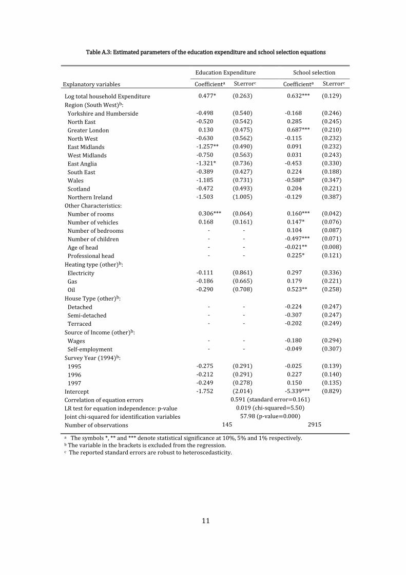
A1.2 The education component of imputed rent
We estimate the share of education in imputed rent, again using, a Heckman procedure. The
estimation results obtained for the two equations by maximum likelihood methods are shown in
Tables A3.
The equation determining the school selection, i.e. private versus state school, is defined as a
function of characteristics of the house (regional location, total rooms, heating, etc), and the
household (number of children, etc) - see complete list in Table A3.
The equation determining the household expenditure on education is specified as function of a
subset of characteristics that are used in the selection equation and a term correcting for the
bias due to sample selection.10
The additional variables excluded from the education expenditure equation and included in the
school selection equation for identification purposes are house type (detached, semi-detached,
terraced), sources of income (wages, self-employment) and other variables (number of bedrooms,
number of children, age of head, profession of head).
As shown in the second last row of Table A.3, several of these variables are significant in the school
selection equation (joint chi-squared for identification variables=57.98, p-value=0.000). Applying
a Hausman test, using the residuals from education expenditure equation, we find the same
variables to have an F-statistic for their joint significance of 1.40 (p=0.18).
After the estimation of the two models predictions about the education expenditure for all
households are constructed by extrapolating the education expenditure for households with
children in state schools from the estimated equation obtained for households with children in
private schools, and multiplying it by the probability that the children in the household attend
private school.
The distribution of the education expenditure as a share of the imputed rent is reported in Table
A.2.
Table A.2: Distribution of the imputed rent and the share of education
Quantiles
1% 5% 10% 25% 50% 75% 90% 95% 99%
Imputed renta 65.6 74.1 79.7 91.3 107.3 126.3 145.9 160.6 185.3
Share of education 0.027 0.036 0.043 0.06 0.083 0.121 0.177 0.222 0.323
Note: a Weekly imputed rent (GBP).
10 Here the error terms from the education expenditure and selection equations are allowed to be correlated, since expenditure on education is observed only for households with children in private schools. These households are likely to be at the top end of the education expenditure distribution, thereby introducing dependence between the school selection and education expenditure equations.
11
Table A.3: Estimated parameters of the education expenditure and school selection equations
Explanatory variables
Education Expenditure
School selection
Coefficienta St.errorc Coefficienta St.errorc
Log total household Expenditure 0.477*** (0.263)
0.632*** (0.129)
Region (South West)b: Yorkshire and Humberside -0.498*** (0.540)
-0.168*** (0.246)
North East -0.520*** (0.542)
0.285*** (0.245)
Greater London 0.130*** (0.475)
0.687*** (0.210)
North West -0.630*** (0.562)
-0.115*** (0.232)
East Midlands -1.257*** (0.490)
0.091*** (0.232)
West Midlands -0.750*** (0.563)
0.031*** (0.243)
East Anglia -1.321*** (0.736)
-0.453*** (0.330)
South East -0.389*** (0.427)
0.224*** (0.188)
Wales -1.185*** (0.731)
-0.588*** (0.347)
Scotland -0.472*** (0.493)
0.204*** (0.221)
Northern Ireland -1.503*** (1.005)
-0.129*** (0.387)
Other Characteristics: Number of rooms 0.306*** (0.064)
0.160*** (0.042)
Number of vehicles 0.168*** (0.161)
0.147*** (0.076)
Number of bedrooms - -
0.104*** (0.087)
Number of children - -
-0.497*** (0.071)
Age of head - -
-0.021*** (0.008)
Professional head - -
0.225*** (0.121)
Heating type (other)b: Electricity -0.111*** (0.861)
0.297*** (0.336)
Gas -0.186*** (0.665)
0.179*** (0.221)
Oil -0.290*** (0.708)
0.523*** (0.258)
House Type (other)b: Detached - -
-0.224*** (0.247)
Semi-detached - -
-0.307*** (0.247)
Terraced - -
-0.202*** (0.249)
Source of Income (other)b: Wages - -
-0.180*** (0.294)
Self-employment - -
-0.049*** (0.307)
Survey Year (1994)b: 1995 -0.275*** (0.291)
-0.025*** (0.139)
1996 -0.212*** (0.291)
0.227*** (0.140)
1997 -0.249*** (0.278) 0.150*** (0.135)
Intercept -1.752*** (2.014)
-5.339*** (0.829)
Correlation of equation errors 0.591 (standard error=0.161)
LR test for equation independence: p-value 0.019 (chi-squared=5.50)
Joint chi-squared for identification variables 57.98 (p-value=0.000)
Number of observations 145
2915
a The symbols *, ** and *** denote statistical significance at 10%, 5% and 1% respectively. b The variable in the brackets is excluded from the regression. c The reported standard errors are robust to heteroscedasticity.

12
A.2 Complete results from the consumer demand and hedonic models
Explanatory variables
Consumer demand
Hedonic
Coefficienta St.errorc
Coefficienta St.errorc
w 0.469*** 0.053
- -
w x (hholds in priv sch.) 0.084*** 0.094
- -
y - -
0.069*** 0.012
y ) x (hholds in priv sch.) - -
-0.015*** 0.019
Chlidren in private schools 0.019*** 0.014
0.248*** 0.031
Ln total expenditure 0.419*** 0.140
0.300*** 0.024
Ln total expenditure sq -0.007*** 0.012
- -
Quantities of goods
Food -0.040*** 0.008
- -
Alcohol and tobacco -0.073*** 0.010
- -
Clothing and footwear -0.015*** 0.005
- -
Fuel and light 0.092*** 0.036
- -
Leisure goods -0.007*** 0.013
- -
Leisure services -0.025*** 0.007
- -
Transport -0.028*** 0.007
- -
Other goods -0.019*** 0.004
- -
Other services -0.051*** 0.018
- -
General Characteristics
Age of head 0.005*** 0.003
0.041*** 0.011
Age of head squared -0.000*** 0.000
-0.000*** 0.000
Number of children 0.025*** 0.011
0.080*** 0.044
Number of children squared 0.001*** 0.002
-0.026*** 0.009
Number of vehicles -0.016*** 0.003
0.045*** 0.013
Number of bedrooms 0.060*** 0.004
0.154*** 0.015
House Type (other)b:
Detached 0.081*** 0.012
0.422*** 0.063
Semi-detached 0.040*** 0.011
0.134*** 0.061
Terraced -0.015*** 0.011
-0.075*** 0.061
Region (South west)b:
Yorkshire and Humberside -0.081*** 0.008
-0.232*** 0.030
North East -0.152*** 0.009
-0.246*** 0.040
Greater London 0.298*** 0.008
0.390*** 0.033
North West 0.083*** 0.008
-0.177*** 0.029
East Midlands -0.152*** 0.009
-0.116*** 0.032
West Midlands -0.112*** 0.008 -0.070** 0.030
East Anglia -0.086*** 0.012
0.027 0.046
South East 0.117*** 0.007
0.224*** 0.024
Wales -0.114*** 0.011
-0.175*** 0.050
Scotland -0.029*** 0.008
-0.207*** 0.036
Northern Ireland -0.339*** 0.018
-0.447*** 0.057
Survey Year (1994)b:
1995 0.015*** 0.005
-0.022*** 0.020
1996 0.093*** 0.006
0.134*** 0.020
1997 0.035*** 0.005
0.088*** 0.020
Intercept 2.045*** 0.418
7.547*** 0.243
Number of observations 2873 -
2873 -
R-Squared 0.865 -
0.609 -
a The symbols *, ** and *** denote statistical significance at 10%, 5% and 1% respectively. b. The variable in the brackets is excluded from the regression. c The reported standard errors are robust to heteroscedasticity.