A Constraint View of IBD Graphs

Rina Dechter, Dan Geiger and Elizabeth Thompson

Donald Bren School of Information and Computer Science

University of California, Irvine, CA 92697

1 Introduction

The report provides a constraint processing view of Identity by decent (IBD) graphs and reformulatesome aspects of the work in [4] from a constraint perspective.

A Bayesian network model of a linkage task can be decomposed into a mixed network that hasa constraint network portion and a Bayesian network portion [3]. It includes selector variables (orinheritance variables) that determine the flow of genes from parents to children along the chromo-some which are described by probabilistic dependencies. We also have the prior probabilities overthe founders. These two sets of probabilistic functions can be regarded as a Bayesian subnetwork.The rest of the dependencies in the model are deterministic and can be viewed as constraints. Ina multimarker model, whenever the selector variables are conditioned on, we have a collection ofindependent small mixed networks, one for each locus. The constraint portion of each locus-basedmixed network, can be processed by a constraint propagation algorithms. In particular, it can beprocessed by arc and path-consistency [1]. We recently observed that if we apply path-consistencysymbolically, (i.e., when the values of the variables (the alleles) are propagated symbolically), thenwe get a tighter constraint network restricted to the founder variables which is equivalent (identical)to the identity by decent (IBD) graph [4].

This equivalent constraint subnetwork together with the probabilistic subnetwork is an equivalentmodel at each locus, conditioned on the selector values. These networks can be far smaller thanthe original ones , and when provided with the actual evidence (the alleles assigned to the typedindividuals), they can often (always?) be solved efficiently. In particular, enumerating the set of allconsistent alleles associated with the founder variables can be done in output linear time. Clearly

1

if the number of consistent founder assignments for a locus-based IBD constraint network is small,computing the probability of evidence conditioned on the selectors s and over all markers can beaccomplished more effectively using the tighter mixed IBD networks than when processing theoriginal one.

The main virtue of the IBD graph seems to be that it changes only locally from one locus to thenext, and only for selectors that represent recombinations [4]. In other words, the IBD constraintnetwork along the chromosome will mimic recombination and will be more a function of the totalnumber of recombinations rather than the number of markers. In this report we propose to use themixed network view of the IBD graph to facilitate constraint-based techniques to advance ideas andgoals in linkage analysis and haplotype computations.

Section 2 provides general background on on mixed probabilistic and deterministic networksand on its use for formulating the linkage analysis task. Section 3 provides the formulation of IBDgraphs.

2 Background: the Mixed network of Linkage analysis

2.1 Definitions

DEFINITION 1 (constraint network) A constraint network CN is a triple CN = ⟨X ,D,C⟩, whereX = {X1, ...,Xn} is a set of variables associated with a set of discrete-valued domains D =

{D1, ...,Dn} and a set of constraints C = {C1, ...,Cr}. Each constraint Ci is a pair ⟨Si,Ri⟩ whereRi is a relation Ri ⊆ DSi defined on a subset of variables Si ⊆ X and DSi is the Cartesian productof the domains of variables Si. The relation Ri denotes all tuples of DSi allowed by the constraint.The projection operator π creates a new relation, πS j(Ri) = {x | x ∈ DS j and ∃y,y ∈ DSi\S j andx∪y ∈ Ri}, where S j ⊆ Si. Constraints can be combined with the join operator 1, resulting in a newrelation, Ri 1 R j = {x | x ∈ DSi∪S j and πSi(x) ∈ Ri and πS j(x) ∈ R j}.

DEFINITION 2 (constraint satisfaction problem, satisfiability) The constraint satisfaction prob-lem (CSP) defined over a constraint network C = ⟨X ,D,C ⟩, is the task of finding a solution, that is,an assignment of values to all the variables x = (x1, ...,xn),xi ∈ Di, such that ∀Ci ∈C,πSi(x) ∈ Ri.The set of all solutions of the constraint network C is sol(C ) =1 R⟩. When the variables are propo-sitional, having values ”0” and ”1” and the constraints are boolean clauses we have the special caseof a cnf formula and the satisfiability task.

2

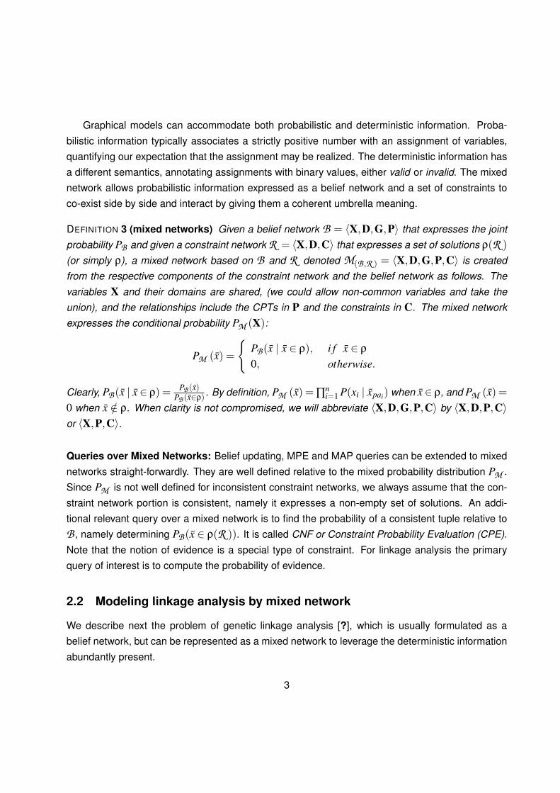
Graphical models can accommodate both probabilistic and deterministic information. Proba-bilistic information typically associates a strictly positive number with an assignment of variables,quantifying our expectation that the assignment may be realized. The deterministic information hasa different semantics, annotating assignments with binary values, either valid or invalid. The mixednetwork allows probabilistic information expressed as a belief network and a set of constraints toco-exist side by side and interact by giving them a coherent umbrella meaning.

DEFINITION 3 (mixed networks) Given a belief network B = ⟨X,D,G,P⟩ that expresses the jointprobability PB and given a constraint network R = ⟨X,D,C⟩ that expresses a set of solutions ρ(R )

(or simply ρ), a mixed network based on B and R denoted M(B,R ) = ⟨X,D,G,P,C⟩ is createdfrom the respective components of the constraint network and the belief network as follows. Thevariables X and their domains are shared, (we could allow non-common variables and take theunion), and the relationships include the CPTs in P and the constraints in C. The mixed networkexpresses the conditional probability PM (X):

PM (x̄) =

{PB(x̄ | x̄ ∈ ρ), i f x̄ ∈ ρ0, otherwise.

Clearly, PB(x̄ | x̄ ∈ ρ) = PB (x̄)PB (x̄∈ρ) . By definition, PM (x̄) = ∏n

i=1 P(xi | x̄pai) when x̄ ∈ ρ, and PM (x̄) =0 when x̄ /∈ ρ. When clarity is not compromised, we will abbreviate ⟨X,D,G,P,C⟩ by ⟨X,D,P,C⟩or ⟨X,P,C⟩.

Queries over Mixed Networks: Belief updating, MPE and MAP queries can be extended to mixednetworks straight-forwardly. They are well defined relative to the mixed probability distribution PM .Since PM is not well defined for inconsistent constraint networks, we always assume that the con-straint network portion is consistent, namely it expresses a non-empty set of solutions. An addi-tional relevant query over a mixed network is to find the probability of a consistent tuple relative toB , namely determining PB(x̄ ∈ ρ(R )). It is called CNF or Constraint Probability Evaluation (CPE).Note that the notion of evidence is a special type of constraint. For linkage analysis the primaryquery of interest is to compute the probability of evidence.

2.2 Modeling linkage analysis by mixed network

We describe next the problem of genetic linkage analysis [?], which is usually formulated as abelief network, but can be represented as a mixed network to leverage the deterministic informationabundantly present.

3

21

3

(a) Pedigree

pG 1,1mG 1,1

pG 1,3pS 1,3

(b) Constraint

pG 1,1mG 1,1

1,1P

pG 1,2mG 1,2

1,2P

pG 1,3mG 1,3

1,3P

pS 1,3mS 1,3

pG 2,1mG 2,1

2,1P

pG 2,2mG 2,2

2,2P

pG 2,3mG 2,3

2,3P

pS 2,3mS 2,3

Locus 1

Locus 2

(c) Mixed network

Figure 1: Genetic linkage analysis

Genetic linkage analysis is a statistical method for mapping genes onto a chromosome, anddetermining the distance between them. This is very useful in practice for identifying disease genes.Without going into the biology details, we briefly describe how this problem can be modeled as areasoning task in a mixed network.

Figure 1(a) shows the simplest pedigree, with two parents (denoted by 1 and 2) and an offspring(denoted by 3). Square nodes indicate males and circles indicate females. Figure 1(c) showsthe usual belief network that models this small pedigree for two particular loci (locations on thechromosome). There are three types of variables, as follows. The G variables are the genotypes(the values are the specific alleles, namely the forms in which the gene may occur on the specificlocus), the P variables are the phenotypes (the observable characteristics). Typically these are

4

evidence variables, and for the purpose of the graphical model they take as value the specificunordered pair of alleles measured for the individual. The S variables are selectors (taking values0 or 1). The upper script p stands for paternal, and the m for maternal. The first subscript numberindicates the individual (the number from the pedigree in 1(a)), and the second subscript numberindicates the locus. The interactions between all these variables are indicated by the arcs in Figure1(c).

Due to the genetic inheritance laws, many of these relationships are actually deterministic. Forexample, the value of a selector variable determines the genotype variable. Formally, if a is thefather and b is the mother of x, then:

Gpx, j =

{Gp

a, j, i f Spx, j = 0

Gma, j, i f Sp

x, j = 1

and,

Gmx, j =

{Gp

b, j, i f Smx, j = 0

Gmb, j, i f Sm

x, j = 1

The CPTs defined above are in fact deterministic, and can be captured by a constraint, whoseconstraint graph is depicted graphically in Figure 1(b). The only real probabilistic information isdefined by the CPTs between selector variables and the prior probabilities of the founders, namelythe individuals having no parents in the pedigree. Figure 2 provides the mixed network formulationof a founder variable (top of Figure), on the bottom left we have the Bayes subnetwork that consistsof three independent variables and on the right there is a constraint subnetwork. Figure 3 describesthe 3 member family formulation as a mixed network.

Genetic linkage analysis is an example of a belief network that contains many deterministic orfunctional relations that can be exploited as constraints. The typical reasoning task is equivalent tocomputing the probability of the evidence, or to maximum probable explanation.

3 A constraint network view of IBD graphs

To describe a constraint formulation of IBD graphs I will use the description of ibd graphs in sec-tion 2.3 of [4]). Paper [4] provides a description of earlier work (by Sobel and Lang (1996) and byKruglyak et. al. (1996)) of what is called distinct-genome-lable (DGL) graph that allow the compu-tation of P(Y•, j|S•, j). Given an assignment to the inheritance variables S•, j in a particular markerlocus j, and a set of distinct labels for each of the two genomes of each founder, the DGL that can

5

Figure 2: A non-founder mixed network

Figure 3: A mixed network for recombination

6

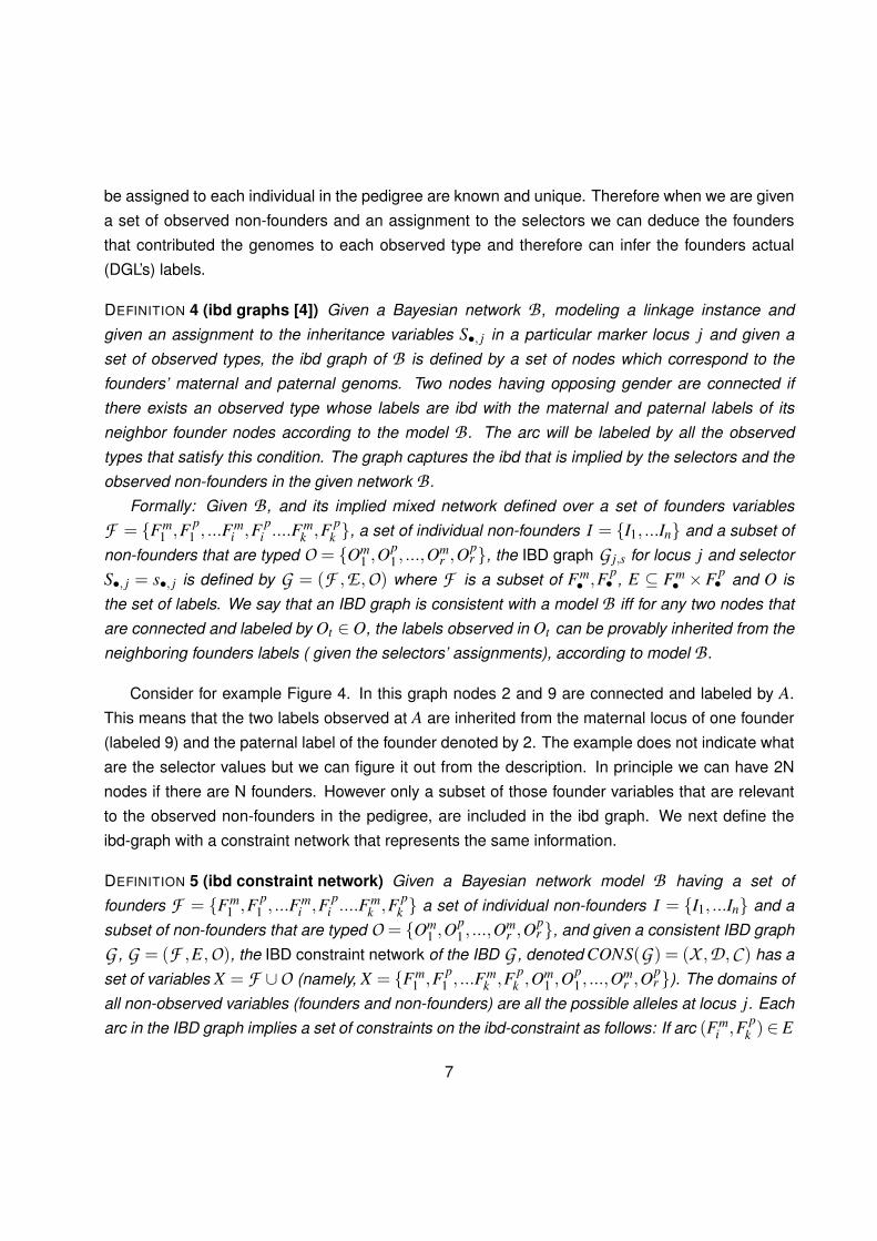
be assigned to each individual in the pedigree are known and unique. Therefore when we are givena set of observed non-founders and an assignment to the selectors we can deduce the foundersthat contributed the genomes to each observed type and therefore can infer the founders actual(DGL’s) labels.

DEFINITION 4 (ibd graphs [4]) Given a Bayesian network B , modeling a linkage instance andgiven an assignment to the inheritance variables S•, j in a particular marker locus j and given aset of observed types, the ibd graph of B is defined by a set of nodes which correspond to thefounders’ maternal and paternal genoms. Two nodes having opposing gender are connected ifthere exists an observed type whose labels are ibd with the maternal and paternal labels of itsneighbor founder nodes according to the model B . The arc will be labeled by all the observedtypes that satisfy this condition. The graph captures the ibd that is implied by the selectors and theobserved non-founders in the given network B .

Formally: Given B , and its implied mixed network defined over a set of founders variablesF = {Fm

1 ,F p1 , ...F

mi ,F p

i ....Fmk ,F p

k }, a set of individual non-founders I = {I1, ...In} and a subset ofnon-founders that are typed O = {Om

1 ,Op1 , ...,O

mr ,O

pr }, the IBD graph G j,s for locus j and selector

S•, j = s•, j is defined by G = (F ,E ,O) where F is a subset of Fm• ,F p

• , E ⊆ Fm• ×F p

• and O isthe set of labels. We say that an IBD graph is consistent with a model B iff for any two nodes thatare connected and labeled by Ot ∈ O, the labels observed in Ot can be provably inherited from theneighboring founders labels ( given the selectors’ assignments), according to model B .

Consider for example Figure 4. In this graph nodes 2 and 9 are connected and labeled by A.This means that the two labels observed at A are inherited from the maternal locus of one founder(labeled 9) and the paternal label of the founder denoted by 2. The example does not indicate whatare the selector values but we can figure it out from the description. In principle we can have 2Nnodes if there are N founders. However only a subset of those founder variables that are relevantto the observed non-founders in the pedigree, are included in the ibd graph. We next define theibd-graph with a constraint network that represents the same information.

DEFINITION 5 (ibd constraint network) Given a Bayesian network model B having a set offounders F = {Fm

1 ,F p1 , ...F

mi ,F p

i ....Fmk ,F p

k } a set of individual non-founders I = {I1, ...In} and asubset of non-founders that are typed O = {Om

1 ,Op1 , ...,O

mr ,O

pr }, and given a consistent IBD graph

G , G = (F ,E,O), the IBD constraint network of the IBD G , denoted CONS(G) = (X ,D,C ) has aset of variables X = F ∪O (namely, X = {Fm

1 ,F p1 , ...F

mk ,F p

k ,Om1 ,O

p1 , ...,O

mr ,O

pr }). The domains of

all non-observed variables (founders and non-founders) are all the possible alleles at locus j. Eacharc in the IBD graph implies a set of constraints on the ibd-constraint as follows: If arc (Fm

i ,F pk )∈ E

7

and is labeled Ol , then there is a constraint over Fmi ,F p

k ,Oml ,O

pl that forces that the maternal and

paternal labels in Ol are identical to one of the values of Fmi and F p

k . Using Boolean constraints ofdisjunction and inequality, these constraints can be expressed as:

Fmi = Om

l ∨Opl , F p

k = Oml ∨Op

l , Fmi ̸= F p

k (1)

The actual alleles for the typed individuals are modeled separately by na evidence domainconstraints. By definition, consistent founder assignments of the IBD graph correspond to solutionsof the IBD-constraint network in conjunction with its evidence domain constraints.

Example 1 Consider the example in Figure 5 of [4]. In defining next the IBD constraint network ofthe ibd graph in Figure 4 we will stay with variable names of founders being numbers and variablenames of observed types being alphabetical. The domains constraints associated with evidencewill be be lower alphabetical. The variables of the constraint network are

X = {1,2,3,4,5,6...18,A,B,C,D,E,F,G,H,J,K,L,V,U,W}

The domains of the numerical variables are the possible alleles at that locus. The constraintsassociated with each arc in the ibd graph are:

2 = Am ∨Ap, 9 = Am ∨Ap, 2 ̸= 9 (2)

2 = Bm ∨Bp, 13 = Bm ∨Bp, 2 ̸= 13, 2 = Jm ∨ Jp, 13 = Jm ∨ Jp, (3)

2 = Gm ∨Gp, 4 = Gm ∨Gp, 2 ̸= 4 (4)

13 = Dm ∨Dp, 4 = Dm ∨Dp, 13 ̸= 4 (5)

13 = Em ∨E p, 6 = Em ∨E p, 13 ̸= 6 (6)

6 =Cm ∨Cp (7)

6 = Hm ∨H p, 15 = Hm ∨H p, 6 ̸= 15 (8)

8

15 = Lm ∨Lp, 17 = Lm ∨Lp, 15 ̸= 17 (9)

15 = Fm ∨F p, 4 = Fm ∨F p, 15 ̸= 4 (10)

In this example we assume the following observations. Non-founders A, B, J are all observed tohave a1a4, type G has a1a6, type D has a4a6, type E has a4a2, C has a2a2, F has a3a6, H has a2a3,and L has a1a3. This will be modeled as evidence constraints in the evidence constraint networkin the form of unary constraints that restricts the variable domains. The evidence constraints are:(DA• stands for the pair of constraints: DAm and DAp )DA• = DB• = DJ• = {a1,a4},DG• = {a1,a6}DD• = {a4,a6},DE• = {a4,a2}DC• = {a2,a2}DF• = {a3,a6}DH• = {a2,a3}DL• = {a1,a3}

For example DD• = {a4,a6} stands for the constraints: Dm = a4 ∨a6, Dp = a4 ∨a6 and Dm ̸=Dp. (or Dm = a4 → Dp = a6 and Dp = a4 → Dm = a6 )

In this example there is a single solution which can be obtained by applying arc-consistencyonce the IBD constraint subproblems is assigned the actual values (the specific alleles observedfor the typed individuals. ) From this information we can infer that the label of 2 is a1; labels 9, and13 are a4; 4 is a6; 6 is a2; 15 is a3, and 17 is a1. The probability of this set of labels is q2

1q2q3q24q6.

3.1 Deriving the IBD constraint networks from the input mixed network

We next show that the locus-based IBD constraint subnetwork can be inferred through path andarc-consistency followed by a removal of irrelevant variables.

A mixed network of a linkage analysis task (decomposed from its Bayes network as describedearlier) yields a collection of locus-based mixed networks, one per locus, defined by all its locus vari-ables. This locus-based networks (which ignores the transition dependencies between the selectorsof successive loci, expresses a probability distribution at each locus. By definition, the probability of

9

Figure 4: An example of pedigree with its associated IBD graph

any consistent tuple, conditioned on the selectors, is proportional over the F and O variables to theproduct of the marginal probabilities in the Bayesian network since the Bayesian network portion isa set of independent variables. In our example instance there is only one tuple of founder variablewhich is consistent with the observations namely: (2 = a1; 9 = a4, 13 = a4; 4 = a6; 6 = a2; 15 = a3,17 = a1), its probability is indeed q2

1q2q3q24q6.

The constraint subnetwork within any locus mixed network, conditioned on its selectors can beprocessed by arc and path-consistency in a symbolic manner without using the specific evidenceyielding an equivalent constraint network. When its variables are restricted to the founder variablesonly it becomes far smaller. We will show that this path-consistent network restricted to the rel-evant founder variables is identical to the IBD constraint network defined earlier. In other words,the IBD constraint networks can be obtained by applying path-consistency over the original set ofconstraints. For a definition of the application of path-consistency and arc-consistency see [1].

DEFINITION 6 (Path-consistency) Given a network of constraints R = (X ,D,C) and given a setof evidence nodes Y = y for Y ⊆ X , we define R′ = PC(R,y) as the network obtained by applyingpath-consistency and arc-consistency to R ∧Y = y. The network R′ is defined on the same set ofvariables as R. The restriction of a network R to a subset of variables Z, is denoted RZ .

Proposition 1 Given a mixed network model M j,s = (B j,s,R j,s) at a locus j,and an assignmentto the selector variables S = s of a linkage problem. Let G j,s denotes its IBD graph conditioned

10

Figure 5: A mixed network represented by the IBD graph

on S = s, then the IBD constraint network CONS(G j,s), is identical to the path and arc-consistentnetwork derived from M j,s. Namely CONS(G j,s) = R′

F where R′ = PC(R j,s).

Proof I think it is correct but need to prove.Hypothesis:1. The IBD constraint graphs are always tractable and yield all solutions in output polynomial time.2. Does applying path and arc-consistency on the IBD-restricted constraint network yield the mini-mal domains and constraints.

Figure 5 shows the original constraint network at a locus (on the left) and the derived IBDconstraint network (on the right).Computing the probability of evidence. Paper [4] demonstrates how to compute the probabilityof trait data Z. The paper notes the difference when computing the probability of marker data (Y )and the probability of computing trait data Z. The trait data, given assignments to the inheritancevariables, depends only on the marker data to the left and right and on the trait model (phenotypegiven genotype). Likewise computing the probability of the trait given the selectors can be accom-plished over the derived mixed networks of the trait locus (including the trait model itself) whichconsists of the derived ibd constraint network and the Bayesian networks (that has a collection ofdisconnected probabilistic tables).

Rephrasing within the mixed network formulation, the probability of the evidence conditioned

11

on the selectors at locus j is the product of probabilities over all assignments of founder variablesthat are consistent with the evidence in the corresponding IBD graph. If the number of consistentfounder assignments is small, computing the probability of evidence conditioned on the selectorsand computing the probability of evidence over all markers can be accomplished along the mixednetworks more effectively. However if we have many markers, as is the case in snps data, or if wehave complex diseases computation may still be difficult.

The main virtue of the IBD graph seems to be that it changes only locally from one locus tothe next, and only for selectors that represent recombinations. In other words, the IBD constraintproblem along the chromosome will mimic recombination and will be more a function of the totalnumber of recombinations rather than the number of markers.

3.2 Moving from one locus to the next capturing recombination: sporadic

thoughts

Assume now that in addition to the selector variables we add persistence variables Q•, j whereQ•, j = 0 if there is no change moving from S•, j to S•,( j+1). In other words Q•, j = |S•, j − S•, j+1|.The number of changes due to recombination moving from one locus to the next is the number of1’s in this Q delta function. We can now add another auxiliary variable that counts the number ofrecombinations moving from one locus to the next called M•, j = ∑i Q•,i, j. We can identify markersof interest as those where some recombination could occur, namely those for whom M is greaterthan 0.

The number of different IBD graphs can be significantly smaller than the number of differentselector combinations along the chromosome. We can also assume that since snps are so close,there could be only a single recombination for a single individual moving in from one snp to the nextand that for some small interval no recombination occurs. This seems to be what is argued in [4]in section 2.4. This is also consistent with assumptions made in Geiger et. al.’s work on handlingSNP data http://cbl-hap.cs.technion.ac.il/superlink-snp/. Section 2.4 also demonstrate how the IBDgraph can change along the chromosome due to recombination.

Compiling IBD constraint graphs. The collection of IBD constraint graphs along the chromosomecan be compiled and allows a far more manageable computation. One option we may consider isto use AND/OR multi-valued decision diagrams [2]. Another option is proposed and carried out in arecent paper [?].

Extension of the mixed network view to inference of identity by descent on two chromosome ofthe same individual as discussed in Section 3 of [4] could also illuminate the computational aspect

12

and can bring in additional constraint processing and general graphical models ideas. In particu-lar, modeling LD along the chromosome can be captured through additional (HMM like) transitionprobabilities between founder variables. Finally extension analyzing chromosome of population,where each individual is captured by its IBD graph along the chromosome are likely to yield farmore informative answers. The mixed probabilistic and constraint-based view of this data can bringto bear both advanced computation developed in the constraint community and graphical modelcommunities.

References

[1] R. Dechter. Constraint Processing. Morgan Kaufmann Publishers, 2003.

[2] R. Mateescu and R. Dechter. Compiling constraint networks into and/or multi-valued decisiondiagrams. In Constraint Porgramming (CP2006), 2006.

[3] Robert Mateescu and Rina Dechter. Mixed deterministic and probabilistic networks. Ann. Math.Artif. Intell., 54(1-3):3–51, 2008.

[4] E. A. Thompson. Analysis of data on related individuals through inference of identity by decent.In Technical report 539, Dept of Statistics, University of Washington, August, 2008.

13