High-order short-time expansions for ATM option prices of exponential

Levy models

Jose E. Figueroa-Lopez∗ Ruoting Gong† Christian Houdre‡

August 18, 2013

Abstract

The short-time asymptotic behavior of option prices for a variety of models with jumps has received muchattention in recent years. In the present work, a novel second-order approximation for ATM option prices is derivedfor a large class of exponential Levy models with or without Brownian component. The results hereafter shed newlight on the connection between both the volatility of the continuous component and the jump parameters andthe behavior of ATM option prices near expiration. In the presence of a Brownian component, the second-orderterm, in time-t, is of the form d2 t

(3−Y )/2, with the coefficient d2 depending only on Y , the degree of jump activity,on σ, the volatility of the continuous component, and on an additional parameter controlling the intensity of the“small” jumps (regardless of their signs). This extends the well known result that the leading first-order term isσt1/2/

√2π. In contrast, under a pure-jump model, the dependence on Y and on the separate intensities of negative

and positive small jumps are already reflected in the leading term, which is of the form d1t1/Y . The second-order

term is shown to be of the form d2t and, therefore, its order of decay turns out to be independent of Y . Theasymptotic behavior of the corresponding Black-Scholes implied volatilities is also addressed. Our method of proofis based on an integral representation of the option price involving the tail probability of the log-return processunder the share measure and a suitable change of probability measure under which the pure-jump component of thelog-return process becomes a Y -stable process. Our approach is sufficiently general to cover a wide class of Levyprocesses which satisfy the latter property and whose Levy densitiy can be closely approximated by a stable densitynear the origin. Our numerical results show that first-order term typically exhibits rather poor performance andthat the second-order term significantly improves the approximation’s accuracy.

AMS 2000 subject classifications: 60G51, 60F99, 91G20, 91G60.

Keywords and phrases: Exponential Levy models; CGMY and tempered stable models; short-time asymptotics;at-the-money option pricing; implied volatility.

1 Introduction

It is generally recognized that the standard Black-Scholes option pricing model is inconsistent with options data, whilestill being used in practice because of its simplicity and the existence of tractable solutions. Exponential Levy modelsgeneralize the classical Black-Scholes setup by allowing jumps in stock prices while preserving the independence andthe stationarity of returns. There are several reasons for introducing jumps in financial modeling. First of all, suddensharp shifts in the price level of financial assets often occur in practice, and these “jumps” are hard to handled withincontinuous-paths models. Second, the empirical returns of financial assets typically exhibit distributions with heavytails and high kurtosis, which again are hard to replicate within purely-continuous frameworks. Finally, market prices of

∗Department of Statistics, Purdue University, West Lafayette, IN, 47907, USA (figueroa@purdue.edu). Research supported in part bythe NSF Grant DMS-0906919 and DMS-1149692.†Department of Mathematics, Rutgers, The State University of New Jersey, Piscataway, NJ, 08904, USA (rgong@math.rutgers.edu).‡School of Mathematics, Georgia Institute of Technology, Atlanta, GA, 30332, USA (houdre@math.gatech.edu). Research supported in

part by the the Simons Foundation grant #246283.

1

vanilla options display skewed implied volatilities (relative to changes in the strikes), in contrast to the classical Black-Scholes model which predicts a flat implied volatility smile. Moreover, the fact that the implied volatility smile andskewness phenomenon become much more pronounced for short maturities is a clear indication of the need for jumpsin the underlying models used to price options. We refer the reader to Cont and Tankov [11] for further motivationson the use of jump processes in financial modeling.

One of the first applications of jump processes in financial modeling originates with Mandelbrot [35], who suggesteda pure-jump stable Levy process to model power-like tails and self-similar behavior in cotton price returns. Merton [38]and Press [41] subsequently considered option pricing and hedging problems under an exponential compound Poissonprocess with Gaussian jumps and an additive independent non-zero Brownian component. A similar exponentialcompound Poisson jump-diffusion model was more recently studied in Kou [30], where the jump sizes are distributedaccording to an asymmetric Laplace law. For infinite activity exponential Levy models, Barndorff-Nielsen [4] introducedthe normal inverse Gaussian (NIG) model, while the extension to the generalized hyperbolic class was studied byEberlein, Keller and Prause [13]. Madan and Seneta [34] introduced the symmetric variance gamma (VG) modelwhile its asymmetric extension was later analyzed in Madan and Milne [33] and Madan, Carr and Chang [32]. Bothmodels are built on Brownian subordination; the main difference being that the log-return process in the NIG modelis an infinite variation process with Cauchy-like behavior of small jumps, while in the VG model the log-price is offinite variation with infinite but relatively low activity of small jumps. The class of “truncated stable” processes wasfirst introduced by Koponen [29]. It was advocated for financial modeling by Cont, Bouchaud and Potters [10] andMatacz [36], and further developed in the context of asset price modeling by Carr, Geman, Madan and Yor [8], whointroduced the terminology CGMY. Nowadays, the CGMY model is considered to be a prototype of the general classof models with jumps and enjoys widespread applicability.

The CGMY model is a particular case of the more general KoBoL class of Boyarchenko and Levendorksii [7], whichin turn is a subclass of the semi-parametric class of tempered stable processes (TSPs) introduced by Rosinski [46]1.TSPs form a rich class with appealing features for financial modeling. One of their most interesting features lies intheir short-time and long-time behaviors. Indeed, denoting by Y ∈ (0, 2) the index of a TSP, L := (Lt)t≥0, it followsthat (

h−1/Y Lht

)t≥0

D−→ (Zt)t≥0 , h→ 0, (1.1)

where Z := (Zt)t≥0 is a strictly Y -stable Levy process andD−→ denotes convergence in distribution. In fact, (1.1)

holds when Y ∈ (0, 1) provided L is driftless, while it holds when Y ∈ (1, 2) regardless of the mean of L. Roughly, (1.1)suggests that the short-time behavior of TSP is akin to that of a stable process, with its heavy-tailed distribution andself-similarity property which are desirable for financial modeling as emphasized, for example, by Mandelbrot [35]. Incontrast, (

h−1/2Lht

)t≥0

D−→ (Wt)t≥0 , h→∞, (1.2)

where (Wt)t≥0 is a Brownian Motion, which suggests that in the long-horizon, the process is Brownian-like. In terms ofincrements, if we were to consider the consecutive “high-frequency” increments of the process L, say Lhi−Lh(i−1)i≥1

with h 1, these will exhibit statistical features consistent with those of a selfsimilar stable time series. But, low-frequency increments, say Lhi − Lh(i−1)i≥1 with h h, will have Gaussian like distributions.

Stemming in part from their importance for model calibration and testing, small-time asymptotics of option priceshave received a lot of attention in recent years (see, e.g., [5], [6], [14], [15], [16], [21], [22], [23], [24], [25], [40], [42],[49]). We shall review here only the studies most closely related to ours, focusing in particular on the at-the-money(ATM) case. Carr and Wu [12] first analyzed, partially via heuristic arguments, the first-order asymptotic behavior ofan Ito semimartingale with jumps. Concretely, [12] argues that ATM option prices of pure-jump models of boundedvariation decrease at the rate O(t), while they are just O(t1/2) in the presence of a Brownian component. By analyzingthe particular case of a stable pure-jump component, [12] also argues that, for other cases, the rate could be O(tβ) forsome β ∈ (0, 1). Muhle-Karbe and Nutz [39] formally showed that, in the presence of a continuous-time component,the leading term of ATM option prices is of order

√t, for a relatively broad class of Ito models, while for a type of

Ito processes with α-stable-like small jumps and α > 1, the leading term is O(t1/α) (see also [16, Proposition 4.2], [17,

1The terminology Tempered Stable is widely used in the literature, but unfortunately there is no uniform usage. It is worth noting thatRosinski’s class ([46]) is much more general than the “tempered stable” class introduced in several classical references of financial modelingwith jumps (e.g. [2], [11], [31]).

2

Theorem 3.7], and [49, Proposition 5] for related results in exponential Levy models). However, none of these papersgive higher order asymptotics for the ATM option prices.

In the present paper, we study the small-time behavior for at-the-money call (or equivalently, put) option prices

E (St − S0)+

= S0E(eXt − 1

)+, (1.3)

under the exponential Levy modelSt := S0e

Xt , (1.4)

where X := (Xt)t≥0 is the superposition of a tempered-stable-like process L := (Lt)t≥0 and of an independent Brownianmotion (σWt)t≥0, i.e.,

Xt := σWt + Lt, (1.5)

where W := (Wt)t≥0 is a standard Brownian motion independent of L. The term “tempered stable” is understoodhere in a much more general sense than in several classical sources of financial mathematics (e.g., [2], [11], [31]) andeven more general than in Rosinski [46]. Roughly (see Section 2 below for the explicit conditions), we consider Levyprocesses whose Levy measure ν admits a density s : R\0 → (0,∞) such that, for some Y ∈ (1, 2), the functionq(x) := s(x)|x|Y+1 satisfies the following fundamental property:

limx0

1

x(C+ − q(x)) = β+, lim

x0

1

x(C− − q(x)) = −β−, (1.6)

for some positive constants C+, C−, β+, β− > 0. Intuitively, (1.6) indicates that the small jumps of the processbehave like those of a Y -stable process. As it turns out (see [44, Proposition 1]), this class still exhibits the appealingshort-time and long-time behaviors of Rosinski’s original tempered stable processes as described in (1.1)-(1.2) above.It is worth noting that the previously defined parameter Y coincides with the Blumenthal-Getoor index BG := infr ≥0 :

∫|x|≤1

|x|rν(dx) < ∞ of the process L, which measures the “degree of jump activity” of the process in that∑u≤t |∆Lu|r <∞, a.s., if and only if r > Y (see, e.g., [48]). As it turns out, for any r > Y > 1, limt→0 t

−1Eψ(Lt) =∫ψ(x)ν(x) for any bounded continuous function ψ such that ψ(x) = O(|x|r) as x→ 0 (see [27]).

Under the standing assumption (1.6) and other mild conditions, we show that the first-order asymptotic behaviorof (1.3) in short-time takes the form

limt→0

t−1/Y E (St − S0)+

= S0E(Z+), (1.7)

where Z is a centered Y -stable random variable under P. When σ 6= 0, Z ∼ N (0, σ2) (i.e., Y = 2) and, thus,E(Z+) = σ/

√2π, as already shown in [49] and [42]. If σ = 0 and L is symmetric, the characteristic function of Z is

explicitly given by

E(eiuZ

)= exp

−2CΓ(−Y )

∣∣∣∣cos

(1

2Y π

)∣∣∣∣ |u|Y,where C := C+ = C− can be interpreted as a measure of the “intensity of small jumps” of the process. In that case,(see [48, (25.6)]),

d1 := E(Z+)

=1

πΓ

(1− 1

Y

)(2CΓ(−Y )

∣∣∣∣cos

(πY

2

)∣∣∣∣)1/Y

. (1.8)

We refer the reader to Remark 3.5 below for the explicit expression of the leading term in the general case. Interestinglyenough, under the presence of a continuous component (σ 6= 0), the first-order asymptotic term only reflects informationon the continuous-time volatility, in sharp contrast with the pure-jump case where the leading term depends on theparameter C and on the index Y , which in turn respectively control the intensity of small jumps and the degree ofjump activity of the process, as already stated above. The intuition behind (1.7) is actually easy to explain. Indeed,since (St − 1)+ =

(eXt − 1

)+

= e(Xt)+ − 1 ∼ (Xt)+, it is expected that

limt→0

t−1/Y E (St − S0)+

= limt→0

E((

t−1/YXt

)+

)= E ((Z1)+) , (1.9)

3

in light of (1.1). Note that in the presence of a non-zero Brownian component, it is known that t−1/2XtD−→ σW1 as

t→ 0 (see [48, pp. 40]).

The asymptotic result (1.7) is in agreement with the result of Tankov [49, Theorem 5], which showed that for apure-jump Levy process (Xt)t≥0 (i.e., σ = 0 in (1.5)), whose characteristic function is of the form

E(eiuXt

)= exp

(tiuγ − |u|Y f(u)

), (1.10)

with Y ∈ (1, 2) and a function f satisfying limu∞ f(u) = c+ ∈ (0,∞) and limu−∞ f(u) = c− ∈ (0,∞), it followsthat

limt→0

t−1/Y E (St − S0)+

=S0

2π

(c1/Y+ + c

1/Y−

). (1.11)

An expression similar to (1.7) is also obtained in [39, Theorem 4.4] for a more general class of pure-jump martingales.Nevertheless, as previously mentioned, none of the these papers obtained second or higher order terms for the ATMoption prices.

The main result of the present paper establishes, for the exponential Levy model described above, a second-ordercorrection term to (1.7). To the best of our knowledge, this is the first second-order result in the literature of exponentialLevy models. We show that the second-order asymptotic behavior of the ATM call option price (1.3) in short-time isof the form

1

S0E (St − S0)

+= d1t

1Y + d2t+ o(t), t→ 0, (1.12)

in the pure-jump case (i.e., σ = 0 in (1.5)), while in the presence of a non-zero independent Brownian component (i.e.,σ 6= 0),

1

S0E (St − S0)

+= d1t

12 + d2t

3−Y2 + o

(t

3−Y2

), t→ 0, (1.13)

for different constants d1 and d2 that we will determine explicitly. To wit, we found that, under the presence of anonzero Gaussian component, the second-order term d2 depends only on the degree of jump activity Y and on theparameter C := (C+ + C−)/2, which measures the net intensity of the small jumps of X (regardless of their sign). Inparticular, it is impossible to discern the difference between C+ and C− at this second-order. In contrast, in a pure-jump case (i.e., σ = 0 in (1.5)) the degree of jump activity of the Levy process is already present in the first-order term.As a byproduct of our asymptotic results for option prices, we also give the asymptotic behavior of the correspondingBlack-Scholes implied volatility, denoted by σ(t). Concretely, we show that, in the presence of a Brownian component(i.e., σ 6= 0 in (1.5)),

σ(t) = σ +(C+ + C−)2−

Y2

Y (Y − 1)Γ

(1− Y

2

)σ1−Y t1−

Y2 + o

(t1−

Y2

), t→ 0, (1.14)

while, in the absence of the continuous component,

σ(t) = σ1t1Y −

12 + σ2t

12 + o(t

12 ), t→ 0, (1.15)

for some constants σ1, σ2 that we will determine explicitly.

The results (1.12)-(1.15) are completely new and, furthermore, in our opinion, they are not quite easy to guessas the first-order term. Indeed, for instance, the intuition behind (1.9) does not seem to be directly transferable to(1.12)-(1.13) since, from the second-order Taylor expansion of the exponential,

(St − 1)+ = e(Xt)+ − 1 ≈ (Xt)+ +1

2X2t

D≈ t1/Y (Z1)+ +

1

2t2/Y Z2

1 ,

where for the third approximation we again used that t−1/YXtD→ Z1 as t→ 0. However, EZ2

1 =∞ and the argumentfails after taking expectations. Our derivation is fully probabilistic and builds on two facts. First, we make use of thefollowing model-free representation due to Carr and Madan [9]:

1

S0E (St − S0)

+= P∗ (Xt > E) =

∫ ∞0

e−xP∗ (Xt > x) dx, (1.16)

4

where P∗ is the martingale probability measure obtained when one takes the stock as the numeraire (i.e., P∗(A) :=E (St1A)) and E is an independent mean-one exponential random variable under P∗. The measure P∗ is also called the

share measure (see [9]). Second, we further change the probability measure P∗ to another probability measure, say P,under which the pure jump-component of X becomes a stable Levy process, independent of the continuous componentof X. This change, in turn, enables us to exploit some key features of stable processes such as self-similarity and theasymptotic behavior of their marginal densities tails.

Let us finish this introductory section with a brief digression on the relevance as well as potential extensions andapplications of our results:

• Levy models are often criticized for their partial ability to fit volatility surfaces across maturities and to accountfor some stylized features of stock prices such as volatility clustering. A natural question is then whether theresults hereafter can be extended to more complex models. The short answer is “yes”. Even though a completeexposition of this point is out of the scope of the present manuscript, we can broadly justify the reason and whythe results obtained in the present paper are crucial for such extensions. The reason has its origins in the work ofMuhle-Karbe and Nut [39], where first-order asymptotics of ATM option prices for a relatively general martingaleprocess with jumps and stochastic volatility are obtained by first showing the analog for a suitable class of Levymodels and then proving that the option prices under the general model can be closely approximated by those ofa suitably chosen Levy model in the class. It is therefore expected that our second-order expansions will be validfor a much more general class of Ito models satisfying certain regularity conditions (cf. [20]). Thus, for instance,it is expected that (1.14) will hold with σ replaced with the spot volatility at time 0, say σ0, which itself can berandom depending on an additional risky factor such as in the Heston model.

• From a qualitative point of view, the short-time expansions stated here enable us to connect information of themodel’s parameters to key features of the option prices and the implied volatility smile or, at a more basic level,allow us to identify (and rank) the parameters (or numerical features of functional parameters) that influencethe most the behavior of the option prices and implied volatilities in short-time. Hence, for instance, (1.14) tellsus that, under a continuous component and an infinite stable-like jump activity component, the most importantfeature that determines the short-time behavior of the implied volatility, below the spot volatility σ, is theintensity of small-jumps as measured by C := (C+ + C−)/2 and that its influence is “felt at the rate” of t1−Y/2,much stronger than how the jump features start to be “felt” in the case of a finite jump activity, where the rateis of order t1/2 (see Remark 4.4 below).

• From a quantitative point of view, as previously mentioned, short-time asymptotics of option prices are relevantin model testing and calibration. The first type of application was already present in the seminal work of Carrand Wu [12]. Regarding the second type of application, high-order expansions, as the ones obtained here, canfacilitate numerical calibration by, e.g., suggesting proper functional forms for extrapolation purposes or settingstarting points of numerical calibration methods. We refer to Remark 4.5 below for more information about thelatter type of application.

The present article is organized as follows. Section 2 introduces the class of Levy processes studied thereafter andsome probability measures transformations, which will be needed throughout the paper. Section 3 establishes thesecond-order asymptotics of the call option price under the pure-jump model (σ = 0). Section 4 establishes the second-order asymptotics of the call option price under an additional independent non-zero Brownian component (σ 6= 0).Section 5 illustrates our second-order asymptotics for the important particular class of CGMY models, recovering ourpreliminary results first presented in [18]. Section 6 assesses the performance of the asymptotic expansions through adetailed numerical analysis for the CGMY model. The proofs of our main results are deferred to the appendices.

2 A tempered-stable-like model with Brownian component

Let L := (Lt)t≥0 be a pure-jump Levy process with triplet (0, b, ν) and let W := (Wt)t≥0 be a Wiener process,independent of L, defined on a complete filtered probability space (Ω,F , (Ft)t≥0,P). We assume zero interest rate andthat P is a martingale measure for the exponential Levy model

St = S0eXt , with Xt := σWt + Lt,

5

where (St)t≥0 represents the price process of a non-dividend paying risky asset. Equivalently, the Levy triplet (σ2, b, ν)of X := (Xt)t≥0 is such that

(i)

∫ ∞1

exν(dx) <∞, and (ii) E(eX1)

= exp

(b+

σ2

2+

∫R0

(ex − 1− x1|x|≤1

)ν(dx)

)= 1, (2.1)

where hereafter R0 := R\0 and the Levy triplets are given relative to the truncation function 1|x|≤1 (see [48,Section 8]). Without loss of generality, we also assume that (Xt)t≥0 is the canonical process Xt(ω) := ω(t) definedon the canonical space Ω = D([0,∞),R) (the space of cadlag functions ω : [0,∞) → R) equipped with the σ-fieldF := σ(Xs : s ≥ 0) and the right-continuous filtration Ft := ∩s>tσ(Xu : u ≤ s)).

As explained in the introduction, we consider a tempered-stable-like Levy processes L where the Levy measureadmits a density s : R0 → [0,∞) of the form

s(x) = |x|−Y−1q(x),

for Y ∈ (1, 2) and a bounded measurable function q : R0 → [0,∞) such that

limx0

1

x(C+ − q(x)) = β+, lim

x0

1

x(C− − q(x)) = −β−, (2.2)

for some positive constants C+, C−, β+ and β−. Throughout, we will also make use of the following assumptions:

Assumption 2.1. The function q : R0 → [0,∞) is such that

(i) q(x) ≤ C−, for all x < 0; (ii) q(x) ≤ C+e−x, for all x > 0; (2.3)

(iii) lim sup|x|→∞

| ln q(x)||x|

<∞; (iv) inf|x|<δ

q(x) > 0, for any δ > 0. (2.4)

A prototypical tempered-stable-like process, as understood here, is the CGMY process of widespread use in math-ematical finance. For the CGMY process,

ν(dx) =

(Ce−Mx

x1+Y1x>0 +

CeGx

|x|1+Y1x<0

)dx, (2.5)

so that C+ = C− = C, β+ = C+M , and β− = C−G. From this analogy, we choose to re-express the model in terms ofthe parameters M := β+/C+ and G := β−/C−, and the function

q(x) :=q(x)

C+1x>0 +

q(x)

C−1x<0. (2.6)

In that case, (2.2) can equivalently be written as

limx0

1

x(1− q(x)) = M, lim

x0

1

x(1− q(x)) = −G. (2.7)

The following relations are direct consequences of (2.7) and are only stated here for future reference:

(i) limδ0

q (δy)1/δ

= e−yM1y>0 + e−|y|G1y<0, (ii) limδ0

1

δln q (δy) = −yM1y>0 − |y|G1y<0, (2.8)

for any y ∈ R\0. Let us also note that (2.3-ii) implies the martingale condition (2.1-i) and also that M > 1.

Remark 2.2. The class of processes considered here is similar to the unifying class of Regular Levy Processes ofExponential type (RLPE) as introduced in [7]. It also covers the class of proper tempered stable processes as definedin [46] as well as several parametric models typically used in mathematical finance, including the CGMY processesand the more general class of normal tempered stable processes (cf. [11, Section 4.4.3]). Let us also remark that therange of Y considered here (namely, Y ∈ (1, 2)) may arguably be the most relevant for financial applications in lightof several recent econometric studies of high-frequency financial data suggesting that the Blumenthal-Getoor index islarger than 1 (cf. [1], [3], and references therein). Nevertheless, admittedly the Blumenthal-Getoor index is in generalrelatively hard to estimate and different, earlier, studies have indicated values of Y < 1 for some financial data set(see, e.g., [8]).

6

Following a density transformation construction as given in Sato [48, Definition 33.4 and Example 33.14] and usingthe martingale condition EeXt = 1, we define a probability measure P∗ on (Ω,F) via

dP∗|FtdP|Ft

= eXt , t ≥ 0, (2.9)

i.e., P∗(B) = E(eXt1B

), for any B ∈ Ft and t ≥ 0. The measure P∗, sometimes termed the share measure, can be

interpreted as the martingale measure when using the stock price as the numeraire. Under this probability measure,(Xt)t≥0 has the representation (σW ∗t +L∗t )t≥0 where, under P∗, W ∗ := (W ∗t )t≥0 is a Wiener process and L∗ := (L∗t )t≥0

is a Levy process with triplet (0, b∗, ν∗) given by

ν∗(dx) := exν(dx) = exs(x)dx, b∗ := b+

∫|x|≤1

x (ex − 1) s(x)dx+ σ2,

which is moreover independent of W ∗. Hereafter, we set

q∗(x) = q(x)ex, s∗(x) = |x|−Y−1q∗(x), q∗(x) := q(x)ex.

The next relations follow immediately from (2.8):

(i) limδ0

q∗ (δy)1/δ

= e−yM∗1y>0 + e−|y|G

∗1y<0, (ii) lim

δ0

1

δln q∗ (δy) = −yM∗1y>0 − |y|G∗1y<0, (2.10)

where

M∗ := M − 1, and G∗ := G+ 1.

An important tool thereafter is to change probability measures from P∗ to another probability measure, hereafterdenoted by P, under which (L∗t )t≥0 is a stable Levy process and (W ∗t )t≥0 is a Wiener process independent of L∗.Concretely, let

q(x) := C+1x>0 + C−1x<0, ν(dx) := |x|−Y−1q(x)dx, b := b∗ +

∫|x|≤1

x(ν − ν∗)(dx).

Note that ν is the Levy measure of a Y -stable Levy process. Moreover, ν is equivalent to ν∗ since clearly ν∗(dx) =exq(x)q(x)−1ν(dx) and q is strictly positive in light of (2.4-iv). For future reference, it is convenient to write ν as

ν(dx) = eϕ(x)ν∗(dx), with ϕ(x) := − ln q∗(x) = − ln q(x)− x.

By virtue of [48, Theorem 33.1], there exists a probability measure P locally equivalent2 to P∗ such that (Xt)t≥0 is a

Levy process with Levy triplet (σ2, b, ν) under P, provided that the following condition is satisfied:∫R0

(eϕ(x)/2 − 1

)2

ν∗(dx) =

∫R0

(1− e−ϕ(x)/2

)2

ν(dx) <∞.

To see that the previous condition holds under our assumptions, note that the integral therein can be expressed as

C+

∫ ∞0

(1− e 1

2 ln q∗(x))2

|x|−Y−1dx+ C−

∫ 0

−∞

(1− e 1

2 ln q∗(x))2

|x|−Y−1dx, (2.11)

and, by (2.10-ii), the integrand in the first integral is such that(e

12 ln q∗(x) − 1

)2

∼ 1

4(ln q∗(x))

2 ∼ (M∗)2

4x2, as x 0.

2Equivalently, there exists a process (Ut)t≥0 such that P∗(B) = E∗(eUt1B), for t ≥ 0 and B ∈ Ft.

7

This shows that the first integral is finite on any interval (0, ε). Outside any neighborhood of the origin, this integralis finite in view of (2.1-i). The second integral in (2.11) can be handled using again (2.10) and the fact that

ϕ(x) = − ln q∗(x) ≥ 0, for any x < 0, (2.12)

as seen from the assumption (2.3-i).

Now that we have established the existence of the probability measure P, let us state some properties and introducesome related terminology. Throughout, E denotes expectation under P. Letting γ := EX1 = EL∗1, we recall that thecentered process (Zt)t≥0, defined by

Zt := L∗t − tγ, (2.13)

is a strictly Y -stable under P and, thus, is also self-similar, i.e.,(t−1/Y Zut

)u≥0

D= (Zu)u≥0, for any t > 0. (2.14)

Let pZ denote the marginal density function of Z1 under P. It is well known (see, e.g., [48, (14.37)] and referencestherein) that

pZ(v) ∼ C±|v|−Y−1, as v → ±∞, respectively. (2.15)

In particular, for any v > 0, as t→ 0,

P (Zt ≥ v) = P(Z1 ≥ t−1/Y v

)∼ tν([v,∞)) = t

C+

Yv−Y , (2.16)

P (Zt ≤ −v) = P(Z1 ≤ −t−1/Y v

)∼ tν((−∞,−v]) = t

C−Yv−Y . (2.17)

The following tail estimate can also be deduced from (2.15) (see Appendix C for its proof):

P(|Z1| ≥ t−1/Y v

)= P (|Zt| ≥ v) ≤ κt|v|−Y , (2.18)

for all v > 0 and 0 < t ≤ 1 and some absolute constant 0 < κ <∞.

Also, of use below, is the following representation of the log density process

Ut := lndP|FtdP∗|Ft

= limε→0

∑s≤t:|∆Xs|>ε

ϕ (∆Xs)− t∫|x|>ε

(eϕ(x) − 1

)ν∗(dx)

, (2.19)

(cf. [48, Theorem 33.2]). The process (Ut)t≥0 can be expressed in terms of the jump-measure N(dt, dx) := #(s,∆Xs) ∈dt× dx of the process (Xt)t≥0 and its compensated measure N(dt, dx) := N(dt, dx)− ν(dx)dt (under P). Indeed,

Ut = limε→0

(∫ t

0

∫|x|>ε

ϕ(x)N(ds, dx)− t∫|x|>ε

(eϕ(x) − 1

)e−ϕ(x)ν(dx)

)

= limε→0

(∫ t

0

∫|x|>ε

ϕ(x)N(ds, dx) + t

∫|x|>ε

(e−ϕ(x) − 1 + ϕ(x)

)ν(dx)

).

Thus, from the definition of the Poisson integral under a compensated Poisson measure as in [28, Theorem 33.2], weget

Ut = Ut + ηt, (2.20)

with

Ut :=

∫ t

0

∫R0

ϕ(x)N(ds, dx), η :=

∫R0

(e−ϕ(x) − 1 + ϕ(x)

)ν(dx). (2.21)

In particular, from the definition of (Ut)t≥0 in (2.19), the process e−Ut is a P-martingale and, thus,

E(e−Ut

)= eηt. (2.22)

8

Remark 2.3. The constant η above (and, therefore, also Ut) is well defined. Indeed, from (2.4-iv) and (2.10-ii),∫|x|≤1

∣∣∣e−ϕ(x) − 1 + ϕ(x)∣∣∣ |x|−Y−1dx ≤ C1

∫|x|≤1

ϕ2(x)|x|−Y−1dx ≤ C2

∫|x|≤1

|x|1−Y dx <∞,

for some constants 0 < C1, C2 <∞. Similarly, from (2.12) and both conditions in (2.4),∫x<−1

∣∣∣e−ϕ(x) − 1 + ϕ(x)∣∣∣ |x|−Y−1dx ≤ C1

∫x<−1

|ϕ(x)||x|−Y−1dx ≤ C2

∫x<−1

|x|−Y dx <∞.

Finally, from (2.1-i) and (2.4), for some constant 0 < C1 <∞,∫x>1

∣∣∣e−ϕ(x) − 1 + ϕ(x)∣∣∣ |x|−Y−1dx ≤ C1

∫x>1

eln q(x)+xx−Y−1dx+

∫x>1

|−1 + ϕ(x)|x−Y−1dx <∞.

The following decomposition of the process X in terms of the compensated measure N(dt, dx) := N(dt, dx)−ν(dx)dtis also of use throughout:

Xt = σW ∗t + Zt + tγ = σW ∗t +

∫ t

0

∫R0

xN(ds, dx) + tγ. (2.23)

The representation (2.23) can be deduced from the Levy-Ito decomposition of the process (Xt)t≥0 (cf. [28, Theorem

13.4 and Corollary 13.7] or [48, Theorem 19.2]) with the stated Levy triplet (0, b, ν) of X under P and where, by

construction, b must be such that E(Xt) = γt.

3 Pure-jump model

In this section, we find the second-order asymptotic behavior for the at-the-money call option prices (1.3) in the pure-jump model (i.e., σ = 0 and Xt = Lt). The proofs of all the results of this section are deferred to Appendix A. Beforestating our first result, we need to rewrite the call option price (1.3) in a suitable form.

Lemma 3.1. With the probability measure P defined in (2.19) and the parameter γ := EX1 = EL∗1,

t−1Y

1

S0E (St − S0)

+= e−(γ+η)t

∫ ∞−γt1−1/Y

e−t1/Y v E

(e−Ut1t−1/Y Zt≥v

)dv. (3.1)

The next two lemmas are crucial to obtain the main result of the section:

Lemma 3.2. In the setting and under the assumptions of Section 2, for any ξ ≥ 0,

(i) limt→0

E(e−ξt

−1/Y (Ut+Zt))

= eηξY

, (ii) limt→0

E(e−ξt

−1/Y Ut)

= eη∗ξY , (3.2)

where η := Γ(−Y )(C+M

Y + C−GY)

and η∗ = Γ(−Y )(C+(M∗)Y + C−(G∗)Y

). In particular, both t−1/Y (Ut + Zt)

and t−1/Y Ut converge to a Y -stable distribution as t→ 0.

Lemma 3.3. In the setting and under the assumptions of Section 2, the following two assertions hold true:

1. For any v > 0,

limt→0

1

tP(Z+t + Ut ≥ v

)=

∫R0

1x−−ln q(x)≥vν(dx). (3.3)

2. There exist constants 0 < κ <∞ and t0 > 0 such that

(i)1

tP(Ut ≥ v

)≤ κv−Y , (ii)

1

tP(Z+t + Ut ≥ v

)≤ κv−Y , (3.4)

for any 0 < t ≤ t0 and v > 0.

9

We are now in a position to establish the main result of this section. The following result gives the second-orderasymptotic behavior of at-the-money call option prices under an exponential tempered stable Levy model.

Theorem 3.4. For the exponential Levy model (1.4) without Brownian component (σ = 0) and under the conditionsof Section 2,

limt→0

t1Y −1

(t−

1Y

1

S0E (St − S0)

+ − E(Z+

1

))= ϑ+ γ P (Z1 ≥ 0) , (3.5)

where, in terms of the function q introduced in (2.6),

ϑ := C+

∫ ∞0

(exq(x)− q(x)− x)x−Y−1dx, (3.6)

γ := EL∗1 = b+C+ + C−Y − 1

+ C+

∫ ∞0

x−Y (1− q(x)) dx+ C−

∫ 0

−∞|x|−Y (1− q(x)) dx. (3.7)

Remark 3.5. The leading term E(Z+

1

)can be explicitly computed via the absolute first moment of Z1 since E |Z1| =

2E(Z+

1

)− E (Z1) = 2E

(Z+

1

). It turns out that

E(Z+

1

)=

1

2E|Z1| =

1

π(C+ + C−)

1Y Γ(−Y )

1Y

∣∣∣∣cos

(Y π

2

)∣∣∣∣ 1Y

Γ

(1− 1

Y

)(1 +

(C+ − C−C+ + C−

)2

tan2

(Y π

2

)) 12Y

× cos

(1

Yarctan

(C+ − C−C+ + C−

tan

(Y π

2

))), (3.8)

(see the proof of [47, (1.2.13)]). In the symmetric case (i.e. C− = C+ = C), (3.8) simplifies to (1.8).

Remark 3.6. From (3.5), it follows that the short-time second-order asymptotic behavior of the ATM call optionprice (1.3) has the form:

1

S0E (St − S0)

+= d1t

1Y + d2t+ o(t), t→ 0, (3.9)

with d1 = E(Z+

1

)given in (3.8) and d2 = ϑ+γP (Z1 ≥ 0). In words, the first-order term only synthesizes information on

the degree of jump activity as measured by Y and on the intensity of small jumps as measured by C+ and C−. However,the second-order term also incorporates some information about the tempering function q. Let us also point out thateven though the parameters M and G introduced in (2.7) do not explicitly show up in the second-order expansion,their existence guarantees that the last two terms in the right-hand side of (3.7) are well-defined. In particular, we seethat the result is expected to be true if M = 0 or G = 0, but not if either M or G is ∞.

We now proceed to study the asymptotic behavior of the corresponding Black-Scholes implied volatilities. Through-out, let σ(t) denote the ATM Black-Scholes implied volatility at maturity t with zero interest rates and dividend yield.The following result gives the asymptotic behavior of σ(t) as t→ 0.

Corollary 3.7. For the exponential Levy model (1.4) without Brownian component, the implied volatility σ has thefollowing small-time behavior:

σ(t) = σ1t1Y −

12 + σ2t

12 + o(t

12 ), t→ 0, (3.10)

where

σ1 :=√

2π E(Z+

1

), σ2 :=

√2π(ϑ+ γP (Z1 ≥ 0)

), (3.11)

and where ϑ and γ are respectively given in (3.6) and (3.7).

10

4 Pure-jump model with a non-zero Brownian component

In this part, we consider the case of a non-zero Brownian component. Concretely, throughout, (Xt)t≥0 is a Levyprocess with triplet (σ2, b, ν) as introduced in Section 2 and σ 6= 0. The first-order asymptotic behavior for the ATMEuropean call options in this mixed model is obtained in [49] using Fourier methods. We give next the second-ordercorrection term for the at-the-money European call option price. As before, we change the probability measure P∗ toP so that Xt = tγ + σW ∗t + Zt, with (Zt)t≥0 a strictly Y -stable Levy process under P (see (2.13)). Recall also that,

under both P∗ and P, W ∗ is still a standard Brownian motion, independent of (Zt)t≥0. We will also make use of thedecompositions (2.20) and (2.23). The proof of the result below is presented in Appendix B.

Theorem 4.1. For the exponential Levy model (1.4) with non-zero Brownian component and under the conditions ofSection 2, the ATM European call option price is such that

limt→0

tY2 −1

(t−

12

1

S0E (St − S0)+ − σE

∗ (W ∗1 )+

)=

C− + C+

2Y (Y − 1)σ1−Y E∗

(|W ∗1 |

1−Y). (4.1)

Remark 4.2. The (1− Y )-centered moment of a standard normal distribution is given by (see, e.g., [48, (25.6)]):

E∗(|W ∗1 |

1−Y)

=2

1−Y2

√π

Γ

(1− Y

2

).

Thus, the second-order asymptotic behavior of the ATM call option price (1.3) in short-time takes the form

1

S0E (St − S0)

+= d1t

12 + d2t

3−Y2 + o

(t

3−Y2

), t→ 0, (4.2)

with

d1 =σ√2π, d2 =

21−Y

2

√π

Γ

(1− Y

2

)(C− + C+)σ1−Y

2Y (Y − 1). (4.3)

The first-order term only synthesizes the information about the continuous volatility parameter σ. In fact, the first-order term of the ATM call option price under the mixed tempered-stable-like model is the same as the one under theBlack-Scholes model. The second-order term further incorporates the information on the degree of jump activity Yand the net intensity of small jumps as measured by the parameter C := C− + C+. However, these two-terms do notreflect the individual intensities of the small negative or positive jumps as measured by the values of C− and C+. Thisfact suggests that it could be useful to consider a third-order approximation. For more information on the latter inthe CGMY model, we refer the reader to [19].

The next proposition provides the small-time asymptotic behavior for the ATM Black-Scholes implied volatilityunder the tempered-stable-like model with non-zero Brownian component. Unlike the pure-jump case, we can onlyderive the first-order asymptotics using Theorem 4.1. The second-order term for the implied volatility requires third-order asymptotics for the ATM call option price. The proof is deferred to Appendix B.

Corollary 4.3. For the exponential Levy model (1.4) with non-zero Brownian component, the implied volatility σ hasthe following small-time behavior:

σ(t) = σ +(C+ + C−)2−

Y2

Y (Y − 1)Γ

(1− Y

2

)σ1−Y t1−

Y2 + o

(t1−

Y2

), t→ 0. (4.4)

Remark 4.4. It is interesting to compare (4.4) with the corresponding asymptotics under the presence of a jumpcomponent L of finite activity (namely, a compound Poisson process). Indeed, [37] argues that, under a relativelystrong technical condition (see Proposition 5 therein for details), the implied volatility is asymptotically σ+I1

√t+O(t),

for a certain constant I1. As we can see, (4.4) implies that σ(t) converges slower under a tempered stable-like infinitejump activity component. In fact, the higher the degree of jump activity, the slower the rate of convergence is and,thus, the stronger is the effect of the intensity of small jumps in the asymptotic behavior of the implied volatility inshort-time.

11

Remark 4.5. As mentioned in the introduction, short-time asymptotics of option prices are relevant in numericalcalibration. Here, we illustrate an approach for this purpose inspired by a method proposed in [37]. As outlined inthe introduction, it is expected that (4.4) is valid under a stochastic volatility model with σ replaced with the spotvolatility at time 0, say σ0, which itself can be random depending on an additional risky factor (see [20] for furtherinformation about this type of results). Now, two major interrelated issues arise. First, the resulting asymptoticformula would involve the unobserved spot volatility, which is changing in time. Thus, apparently the calibrationwill have to be carried out day by day, but unfortunately, a limited number of short-term options are available inthe market at a any given day. To overcome these issues, we argue as follows: First, it is reasonable that observedprices of options “sufficiently close-to-the-money” can be considered as being at-the-money. Hence, if κ denotes thelog-moneyness ln (K/S0) of the option and σ(t;κ) denotes the corresponding implied volatility under the model, thenwe expect that

σ(t;κ) ≈ σ0 +(C+ + C−)2−Y

Y (Y − 1)Γ

(1− Y

2

)σ1−Y

0 t1−Y2 , (4.5)

when κ ≈ 0. Next, we consider the observed implied volatility corresponding to the close-to-the-money option, hereafterdenoted by σ∗ and solve the equation

σ∗ = σ0 +(C+ + C−)2−Y

Y (Y − 1)Γ

(1− Y

2

)σ1−Y

0 t1−Y2 , (4.6)

for the spot volatility σ0. We denote the smallest of the solutions σ0 by σ0 (t, σ∗;C+, C−, Y ). Then, we substitute thisin (4.5) to get the equation:

σ(t;κ) ≈ σ0 (t, σ∗;C+, C−, Y ) +(C+ + C−)2−Y

Y (Y − 1)Γ

(1− Y

2

)σ0 (t, σ∗;C+, C−, Y )

1−Yt1−

Y2 , (4.7)

which is free of the unobserved spot volatility σ0. Finally, we can calibrate (4.7) to other sufficiently close-to-the-money implied volatilities by minimizing a weighted sum of squared errors. As in [37], this approach has the advantageof enabling us to calibrate the parameters across calendar dates simultaneously and not day by day. Note that,alternatively, one can plug σ0(t, σ∗;C+, C−, Y ) into other type of asymptotics such as the out-of-the-money asymptoticsobtained in [17].

5 Asymptotics for ATM option prices under a CGMY model

In this section, we specialize the second-order asymptotic expansions of the two previous sections to the CGMY model.The result presented here were first reported in [18]. Recall that under the CGMY model, the Levy measure of thepure-jump component (Lt)t≥0 is given by

ν(dx) = |x|−Y−1q(x)dx = |x|−Y−1(Ce−Mx 1x>0 + CeGx 1x<0

)dx, (5.1)

with corresponding parameters C, G, M > 0 and Y ∈ (1, 2). Then, the characteristic function of the log-return processXt = σWt + Lt takes the form

ϕt(u) = E(eiuXt

)= exp

(t

[icu− σ2u2

2+ CΓ(−Y )

((M − iu)Y + (G+ iu)Y −MY −GY

)]), (5.2)

for a constant c ∈ R. The martingale condition (2.1) implies that M > 1 and

c = −CΓ(−Y )((M − 1)Y + (G+ 1)Y −MY −GY

)− σ2

2, (5.3)

(see, e.g., [49, Proposition 4.2]). In particular, the center γ := EX1 = EL1 of X and the parameter b of X (relative tothe truncation function x1|x|≤1) are given by

γ = c− CY Γ(−Y )(MY−1 −GY−1

), b = c−

∫|x|>1

xν(dx)− CY Γ(−Y )(MY−1 −GY−1

).

12

Under the share measure P∗ introduced in Section 2, (Xt)t≥0 has Levy triplet (b∗, (σ∗)2, ν∗) given by

σ∗ := σ, b∗ := c+ σ2 −∫|x|>1

xν∗(dx)− CY Γ(−Y )(

(M∗)Y−1 − (G∗)

Y−1), ν∗(dx) := exν(dx), (5.4)

with M∗ = M − 1 and G∗ = G+ 1. Under the probability measure P, the centered process (Zt)t≥0 is symmetric, and

its center γ := EX1 = EL∗1 is given by (see [18] for the detailed computation)

γ = b+

∫|x|>1

xν(dx) = b∗ +

∫|x|≤1

x(ν − ν∗)(dx) +

∫|x|>1

xν(dx)

= −CΓ(−Y )((M − 1)Y + (G+ 1)Y −MY −GY

)+σ2

2. (5.5)

We also need the value of η defined in (2.21), which, under the CGMY model, is now given by

η = C

∫ ∞0+

(e−M

∗x− 1 +M∗x)x−Y−1dx+ C

∫ 0−

−∞

(eG∗x− 1−G∗x

)|x|−Y−1dx = CΓ(−Y )

((M∗)

Y+(G∗)

Y), (5.6)

where, for the last equality above, we used the analytic continuation of [48, (14.19)].

We are now ready to explicitly write the second-order expansions. First, let us compute the term ϑ of (3.6). Tothis end, it is convenient to use the representation given in (A.17) below noting that in the CGMY case q(x) :=e−Mx1x>0 + eGx1x<0. Hence,

ϑ = C

∫ ∞0

(e−v − 1

) ∫R0

1x−−ln q(x)≥v|x|−Y−1dxdv

= C

∫ ∞0

(e−v − 1

) ∫ ∞0

1Mx≥vx−Y−1dxdv + C

∫ ∞0

(e−v − 1

) ∫ 0

−∞1−x−Gx≥v(−x)−Y−1dxdv

=C

Y

(MY + (G+ 1)Y

) ∫ ∞0

(e−v − 1

)v−Y dv

= −CΓ(−Y )(

(M∗ + 1)Y

+ (G∗)Y), (5.7)

where in the last equality we used the identities∫∞

0(e−v − 1) v−Y dv = Γ(1−Y ) = −Y Γ(−Y ) (see [48, (14.18)]). Using

(5.5)-(5.7) and recalling that ϑ = ϑ+ η (see (A.18)), it follows that in the pure-jump CGMY model,

d2 := ϑ+ η +γ

2=CΓ(−Y )

2

((M − 1)Y −MY − (G+ 1)Y +GY

),

while in the general CGMY model with non-zero Brownian component, C+ = C− = C, and thus

d2 :=Cσ1−Y 2

1−Y2

Y (Y − 1)√π

Γ

(1− Y

2

).

6 Numerical examples

In this part, we assess the performance of the previous approximations through a detailed numerical analysis for theCGMY model.

6.1 The numerical methods

Let us first select a suitable numerical scheme to compute the ATM option prices by considering two methods: In-verse Fourier Transform (IFT) and Monte Carlo (MC). Before introducing the IFT, let us set some notations. Thecharacteristic function corresponding to the Black-Scholes model with volatility Σ is given by

ϕBS,Σt (v) = exp

(−Σ2t

2

(v2 + iv

)).

13

The corresponding call option price at the log-moneyness k = log(S0/K) under the Black-Scholes model with volatilityΣ is denoted by CΣ

BS(k); that is,

CΣBS(k) = S0e

−rt E(e(r−Σ2/2)t+ΣWt − ek

)+.

Let us also recall that the characteristic function, under the mixed CGMY model with a Brownian component, isdenoted by ϕt (see (5.2)) and let us denote the corresponding call option price at log-moneyness k by C(k). The IFTmethod is based on the following inversion formula (see [11, Section 11.1.3]):

zT

(k) := C(k)− CΣBS(k) =

1

2π

∫ ∞−∞

e−ivkζT

(v)dv, (6.1)

where

ζT

(v) := eivrϕT

(v − i)− ϕBS,ΣT

(v − i)iv(1 + iv)

. (6.2)

In our case, we fix r = 0 and, since we are only interested in ATM option prices, we set k = 0. In order to computenumerically the integral in (6.1), we use Simpson’s rule:

zT

(0) :=1

2π

∫ ∞−∞

ζT

(v)dv = ∆

P−1∑m=0

w∗MζT (v∗M ) ,

with ∆ = Q/(P − 1), v∗M = −Q/2 +m∆, and w0 = 1/2, w2`−1 = 4/3, and w2` = 2/3, for ` = 1, . . . , P/2.

We now introduce a Monte Carlo method based on the risk-neutral option price representation under the probabilitymeasure P. Under this probability measure and using the notation (2.21) as well as the relations (2.20) and (2.23), wehave:

E(eXT − 1

)+=E∗

(e−XT

(eXT − 1

)+)= E

(e−UT

(1− e−XT

)+)= E

(e−M

∗U+T +G∗U−T −ηT

(1− e−U

+T −U

−T −T γ−σWT

)+),

which can be easily computed by Monte Carlo method using that, under P, the variables U+T and −U−T are independent

Y -stable random variables with scale, skewness, and location parameters TC| cos(πY/2)|Γ(−Y ), 1 and 0, respectively.Standard simulation methods are available to generate stable random variables.

Next, we take the following set of parameters

C = 0.5, G = 2, M = 3.6, Y = 1.5.

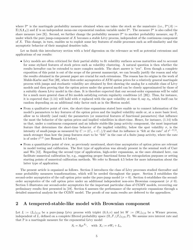
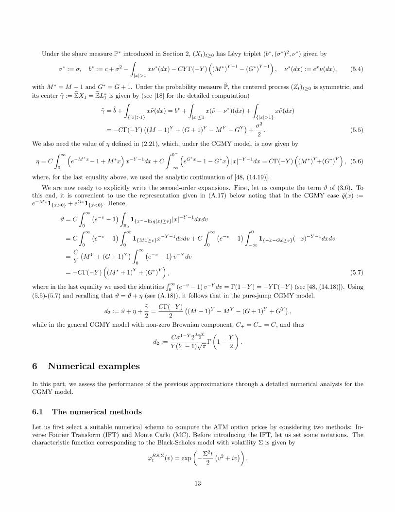
Figure 1 compares the first- and second-order approximations as given in Remarks 3.6 and 4.2 to the prices basedon the Inverse Fourier Transform (IFT-based price) and the Monte Carlo method (MC-based price) under both thepure-jump case and the mixed CGMY case with σ = 0.4. For the MC-based price, we use 100, 000 simulations, whilefor the IFT-based method, we use P = 214 and Q = 800. As it can be seen, it is not easy to integrate numerically thecharacteristic function (6.2) since T is quite small and, therefore, the characteristic functions ϕT and ϕBS,ΣT are quiteflat. The Monte Carlo method turns out to be much more accurate and faster. It is also interesting to note that thesecond-order approximation is in general much more accurate in the pure-jump model than in the mixed model withnonzero continuous component. This observation is consistent with the last comment of Remark 4.2.

6.2 Results for different parameter settings

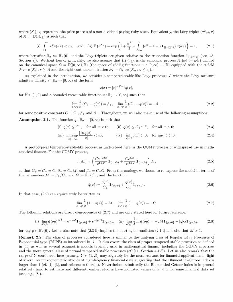
Below, we investigate the performance of the approximations for different settings of parameters:

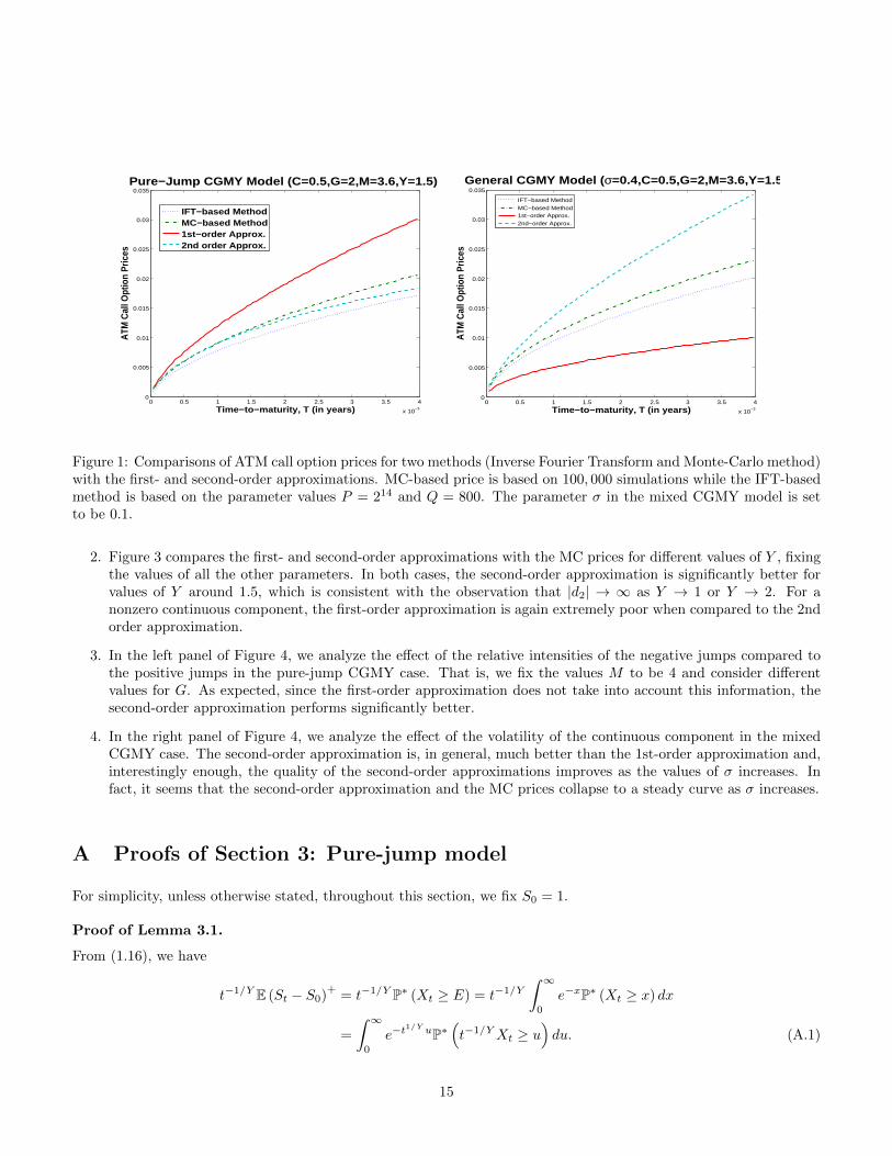
1. Figure 2 compares the first- and second-order approximations with the MC prices for different values of C, fixingthe values of all the other parameters. In the pure-jump case, the second-order approximation is significantlybetter for moderately small values of C, but for larger values of C, this is not the case unless T is extremelysmall. For a nonzero continuous component, the first-order approximation is extremely poor as it only takes intoaccount the parameter σ.

14

0 0.5 1 1.5 2 2.5 3 3.5 4

x 10−3

0

0.005

0.01

0.015

0.02

0.025

0.03

0.035Pure−Jump CGMY Model (C=0.5,G=2,M=3.6,Y=1.5)

Time−to−maturity, T (in years)

ATM

Cal

l Opt

ion

Pric

es

IFT−based MethodMC−based Method1st−order Approx.2nd order Approx.

0 0.5 1 1.5 2 2.5 3 3.5 4

x 10−3

0

0.005

0.01

0.015

0.02

0.025

0.03

0.035

General CGMY Model ( σ=0.4,C=0.5,G=2,M=3.6,Y=1.5)

Time−to−maturity, T (in years)

ATM

Cal

l Opt

ion

Pric

es

IFT−based MethodMC−based Method1st−order Approx.2nd−order Approx.

Figure 1: Comparisons of ATM call option prices for two methods (Inverse Fourier Transform and Monte-Carlo method)with the first- and second-order approximations. MC-based price is based on 100, 000 simulations while the IFT-basedmethod is based on the parameter values P = 214 and Q = 800. The parameter σ in the mixed CGMY model is setto be 0.1.

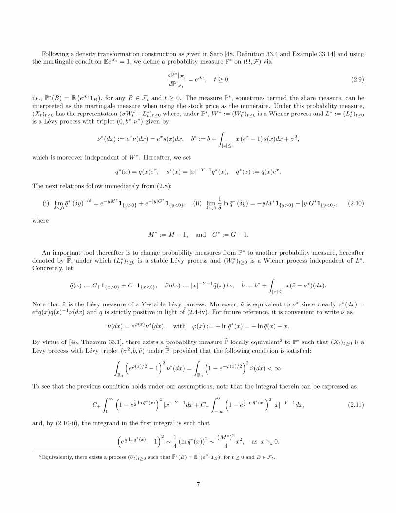
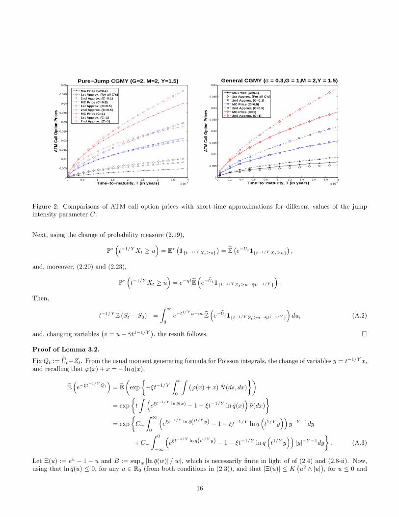
2. Figure 3 compares the first- and second-order approximations with the MC prices for different values of Y , fixingthe values of all the other parameters. In both cases, the second-order approximation is significantly better forvalues of Y around 1.5, which is consistent with the observation that |d2| → ∞ as Y → 1 or Y → 2. For anonzero continuous component, the first-order approximation is again extremely poor when compared to the 2ndorder approximation.

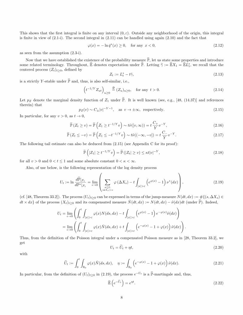
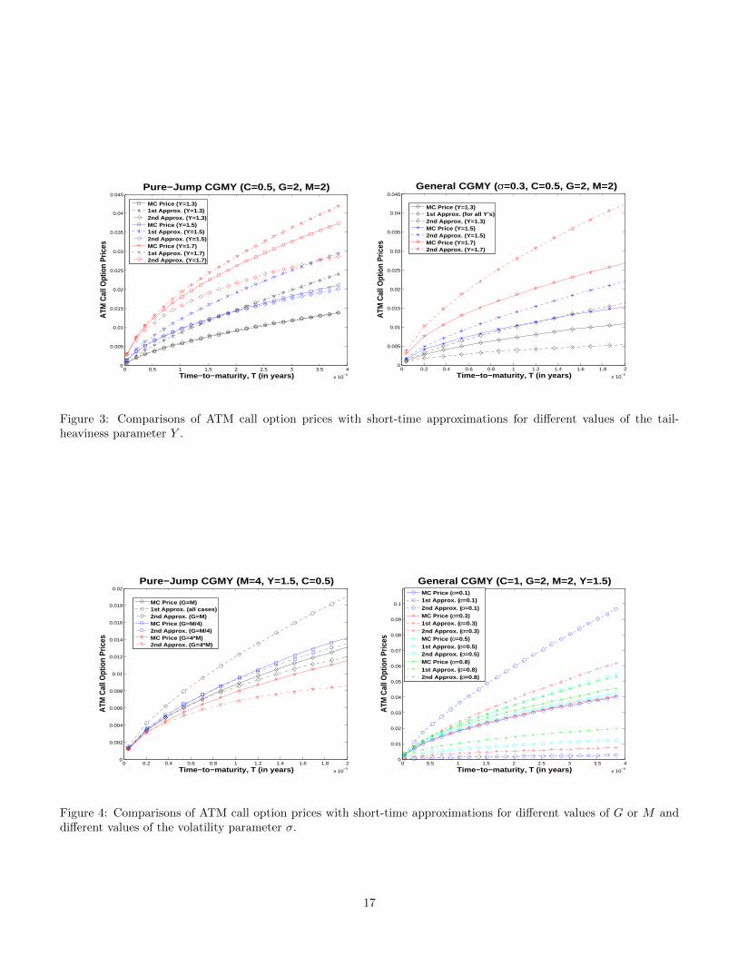
3. In the left panel of Figure 4, we analyze the effect of the relative intensities of the negative jumps compared tothe positive jumps in the pure-jump CGMY case. That is, we fix the values M to be 4 and consider differentvalues for G. As expected, since the first-order approximation does not take into account this information, thesecond-order approximation performs significantly better.

4. In the right panel of Figure 4, we analyze the effect of the volatility of the continuous component in the mixedCGMY case. The second-order approximation is, in general, much better than the 1st-order approximation and,interestingly enough, the quality of the second-order approximations improves as the values of σ increases. Infact, it seems that the second-order approximation and the MC prices collapse to a steady curve as σ increases.

A Proofs of Section 3: Pure-jump model

For simplicity, unless otherwise stated, throughout this section, we fix S0 = 1.

Proof of Lemma 3.1.

From (1.16), we have

t−1/Y E (St − S0)+

= t−1/Y P∗ (Xt ≥ E) = t−1/Y

∫ ∞0

e−xP∗ (Xt ≥ x) dx

=

∫ ∞0

e−t1/Y uP∗

(t−1/YXt ≥ u

)du. (A.1)

15

0 0.5 1 1.5 2 2.5 3 3.5 4

x 10−3

0

0.005

0.01

0.015

0.02

0.025

0.03

0.035

0.04

0.045

0.05Pure−Jump CGMY (G=2, M=2, Y=1.5)

Time−to−maturity, T (in years)

ATM

Cal

l Opt

ion

Pric

es

MC Price (C=0.1)1st Approx. (for all C’s)2nd Approx. (C=0.1)MC Price (C=0.5)1st Approx. (C=0.5)2nd Approx. (C=0.5)MC Price (C=1)1st Approx. (C=1)2nd Approx. (C=1)

0 0.2 0.4 0.6 0.8 1 1.2 1.4 1.6 1.8 2

x 10−3

0

0.005

0.01

0.015

0.02

0.025

0.03

0.035

0.04

General CGMY ( σ = 0.3,G = 1,M = 2,Y = 1.5)

Time−to−maturity, T (in years)

ATM

Cal

l Opt

ion

Pric

es

MC Price (C=0.1)1st Approx. (For all C’s)2nd Approx. (C=0.1)MC Price (C=0.5)2nd Approx. (C=0.5)MC Price (C=1)2nd Approx. (C=1)

Figure 2: Comparisons of ATM call option prices with short-time approximations for different values of the jumpintensity parameter C.

Next, using the change of probability measure (2.19),

P∗(t−1/YXt ≥ u

)= E∗

(1t−1/YXt≥u

)= E

(e−Ut1t−1/YXt≥u

),

and, moreover, (2.20) and (2.23),

P∗(t−1/YXt ≥ u

)= e−ηtE

(e−Ut1t−1/Y Zt≥u−γt1−1/Y

).

Then,

t−1/Y E (St − S0)+

=

∫ ∞0

e−t1/Y u−ηt E

(e−Ut1t−1/Y Zt≥u−γt1−1/Y

)du, (A.2)

and, changing variables(v = u− γt1−1/Y

), the result follows.

Proof of Lemma 3.2.

Fix Qt := Ut+Zt. From the usual moment generating formula for Poisson integrals, the change of variables y = t−1/Y x,and recalling that ϕ(x) + x = − ln q(x),

E(e−ξt

−1/YQt)

= E(

exp

−ξt−1/Y

∫ t

0

∫(ϕ(x) + x) N(ds, dx)

)= exp

t

∫ (eξt−1/Y ln q(x) − 1− ξt−1/Y ln q(x)

)ν(dx)

= exp

C+

∫ ∞0

(eξt−1/Y ln q(t1/Y y) − 1− ξt−1/Y ln q

(t1/Y y

))y−Y−1dy

+C−

∫ 0

−∞

(eξt−1/Y ln q(t1/Y y) − 1− ξt−1/Y ln q

(t1/Y y

))|y|−Y−1dy

. (A.3)

Let Ξ(u) := eu − 1 − u and B := supw |ln q(w)| /|w|, which is necessarily finite in light of of (2.4) and (2.8-ii). Now,using that ln q(u) ≤ 0, for any u ∈ R0 (from both conditions in (2.3)), and that |Ξ(u)| ≤ K

(u2 ∧ |u|

), for u ≤ 0 and

16

0 0.5 1 1.5 2 2.5 3 3.5 4

x 10−3

0

0.005

0.01

0.015

0.02

0.025

0.03

0.035

0.04

0.045

Time−to−maturity, T (in years)

ATM

Cal

l Opt

ion

Pric

es

Pure−Jump CGMY (C=0.5, G=2, M=2)

MC Price (Y=1.3)1st Approx. (Y=1.3)2nd Approx. (Y=1.3)MC Price (Y=1.5)1st Approx. (Y=1.5)2nd Approx. (Y=1.5)MC Price (Y=1.7)1st Approx. (Y=1.7)2nd Approx. (Y=1.7)

0 0.2 0.4 0.6 0.8 1 1.2 1.4 1.6 1.8 2

x 10−3

0

0.005

0.01

0.015

0.02

0.025

0.03

0.035

0.04

0.045

Time−to−maturity, T (in years)AT

M C

all O

ptio

n Pr

ices

General CGMY ( σ=0.3, C=0.5, G=2, M=2)

MC Price (Y=1.3)1st Approx. (for all Y’s)2nd Approx. (Y=1.3)MC Price (Y=1.5)2nd Approx. (Y=1.5)MC Price (Y=1.7)2nd Approx. (Y=1.7)

Figure 3: Comparisons of ATM call option prices with short-time approximations for different values of the tail-heaviness parameter Y .

0 0.2 0.4 0.6 0.8 1 1.2 1.4 1.6 1.8 2

x 10−3

0

0.002

0.004

0.006

0.008

0.01

0.012

0.014

0.016

0.018

0.02Pure−Jump CGMY (M=4, Y=1.5, C=0.5)

Time−to−maturity, T (in years)

ATM

Cal

l Opt

ion

Pric

es

MC Price (G=M)1st Approx. (all cases)2nd Approx. (G=M)MC Price (G=M/4)2nd Approx. (G=M/4)MC Price (G=4*M)2nd Approx. (G=4*M)

0 0.5 1 1.5 2 2.5 3 3.5 4

x 10−3

0

0.01

0.02

0.03

0.04

0.05

0.06

0.07

0.08

0.09

0.1

General CGMY (C=1, G=2, M=2, Y=1.5)

Time−to−maturity, T (in years)

ATM

Cal

l Opt

ion

Pric

es

MC Price (σ=0.1)1st Approx. ( σ=0.1)2nd Approx. ( σ=0.1)MC Price (σ=0.3)1st Approx. ( σ=0.3)2nd Approx. ( σ=0.3)MC Price (σ=0.5)1st Approx. ( σ=0.5)2nd Approx. ( σ=0.5)MC Price (σ=0.8)1st Approx. ( σ=0.8)2nd Approx. ( σ=0.8)

Figure 4: Comparisons of ATM call option prices with short-time approximations for different values of G or M anddifferent values of the volatility parameter σ.

17

some constant 0 < K <∞,

Ξ(ξt−

1Y ln q

(t

1Y y))|y|−Y−1 ≤ K

((ξt−

1Y ln q

(t

1Y y))2

∧∣∣∣ξt− 1

Y ln q(t

1Y y)∣∣∣) |y|−Y−1

≤ K(

(ξyB)2 ∧ |ξyB|

)|y|−Y−1

≤ K(

(ξB)2 ∨ |ξB|

) (y2 ∧ |y|

)|y|−Y−1,

which is integrable. Therefore, one can pass the limit inside the integrals in (A.3) and, using (2.8),

limt→0

E(e−ξt

−1/YQt)

= exp

C+

∫ ∞0

(e−yξM − 1 + yξM

)y−Y−1dy + C−

∫ 0

−∞

(e−|y|ξG − 1 + |y|ξG

)|y|−Y−1dy

= exp

(C+

∫ ∞0

(e−uM − 1 + uM

)u−Y−1du+ C−

∫ 0

−∞

(e−|u|G − 1 + |u|G

)|u|−Y−1du

)ξY.

Finally, using the analytic continuation of the representation [48, (14.19)], we show that the last expression is of theform exp(ηξY ), with η given as in the statement of the lemma.

For (3.2-ii), we proceed as above to get

E(e−ξt

−1/Y Ut)

=exp

C+

∫ ∞0

Ξ(ξt−1/Y ln q∗

(t1/Y y

))y−Y−1dy + C−

∫ 0

−∞Ξ(ξt−1/Y ln q∗

(t1/Y y

))|y|−Y−1dy

. (A.4)

Now, for all y ∈ R0,

ξt−1/Y ln q∗(t1/Y y

)= ξt−1/Y ln q

(t1/Y y

)+ ξy = ξy

(1

yt1/Yln q

(t1/Y y

)+ 1

)≤ 0, (A.5)

from both conditions in (2.3). Using (A.5), we can then proceed as above to justify passing the limit into the integralsin (A.4). Next, using (2.10), we conclude that

limt→0

E(e−ξt

−1/Y Ut)

= exp

C+

∫ ∞0

(e−yξM

∗− 1 + yξM∗

)y−Y−1dy + C−

∫ 0

−∞

(e−|y|ξG

∗− 1 + |y|ξG∗

)|y|−Y−1dy

= exp

(C+

∫ ∞0

(e−uM

∗− 1 + uM∗

)u−Y−1du+ C−

∫ 0

−∞

(e−|u|G

∗− 1 + |u|G∗

)|u|−Y−1du

)ξY.

Finally, (3.2-ii) follows once more from the analytic continuation of [48, (14.19)].

Proof of Lemma 3.3.

We use a small/large jump type decomposition. Concretely, fix ε > 0 and let

Z(ε)t :=

∫ t

0

∫|x|≥ε

xN(ds, dx), Z(ε)t := Zt − Z(ε)

t . (A.6)

Under P, Z(ε) is a drift-less Levy process with finite Levy measure 1x≥εν(dx) and, thus, is a compound Poisson

process. Denote respectively by (N(ε)t )t≥0 and (ξ

(ε)i )i≥1 the counting process and the sizes of the jumps of (Z

(ε)t )t≥0,

so that Z(ε)t =

∑N(ε)t

i=1 ξ(ε)i . In particular, N (ε) is a Poisson process with intensity λε := EN (ε)

1 and (ξ(ε)i )i≥1 are i.i.d,

random variables with distribution 1|x|≥εν(dx)/λε. Next, defined the corresponding processes for U :

¯U

(ε)

t :=

∫ t

0

∫|x|≥ε

ϕ(x)N(ds, dx) = −N

(ε)t∑i=1

ln q∗(ξ

(ε)i

), U

(ε)t := Ut −

¯U

(ε)

t . (A.7)

We prove the validity of the two assertions in two steps:

18

(1) Recalling that N(ε)t is Poisson distributed with mean λεt and using (A.6) and (A.7), we condition on N

(ε)t to get

t−1P(Z+t + Ut ≥ v

)= t−1P

Z(ε)

t +

N(ε)t∑i=1

ξ(ε)i

+

+ U(ε)t −

N(ε)t∑i=1

ln q∗(ξ

(ε)i

)≥ v

=

1

tP((

Z(ε)t

)+

+ U(ε)t ≥ v

)e−λεt+e−λεtλεP

((Z

(ε)t + ξ

(ε)1

)+

+ U(ε)t − ln q∗

(ξ

(ε)1

)≥ v)

+O(t).

The first term above can be made O(t) by taking ε ∈ (0, ε0), for some small enough ε0 > 0 (see, e.g., [48, Section

26] and [45, Lemma 3.2]). Indeed, first note that the support of the Levy measures of Z(ε) and U (ε) are respectivelyx : |x| ≤ ε and ϕ(x) : |x| ≤ ε = − ln q(x) − x : |x| ≤ ε. Next, since limx→0 q(x) = 1, one can choose εsmall enough so that the supports are contained in a ball of arbitrarily small radius δ, which in turn implies that

P(Z

(ε)t ≥ v/2

)= O(t2) and P

(U

(ε)t ≥ v/2

)= O(t2), by taking δ > 0 small enough. For the second term, first from

(2.7), there exists ε0 > 0 such that, for all 0 < ε < ε0,

a0(v):= λεP((

ξ(ε)1

)+

− ln q∗(ξ

(ε)1

)≥ v)

=

∫R0

1x+−ln q∗(x)≥vν(dx) =

∫R0

1x−−ln q(x)≥vν(dx)

= C+

∫ ∞0

1− ln q(x)≥vx−Y−1dx+ C−

∫ 0

−∞1−x−ln q(x)≥v|x|−Y−1dx,

where for the second equality we recalled that ξ(ε)i has distribution 1|x|≥εν(dx)/λε. Also, since

Fv,ε(z, u) := P((

z + ξ(ε)1

)+

+ u− ln q∗(ξ

(ε)1

)≥ v),

is continuous at (z, u) = (0, 0), for any fixed 0 < ε < ε0, the function

At(v) := t−1P(Z+t + Ut ≥ v

)− a0(v),

is such that

limt→0

At(v) = λε limt→0

(P((

Z(ε)t + ξ

(ε)1

)+

+ U(ε)t − ln q∗

(ξ

(ε)1

)≥ v)− λεP

((ξ

(ε)1

)+

− ln q∗(ξ

(ε)1

)≥ v))

= λε limt→0

E(Fv,ε

(Z

(ε)t , U

(ε)t

)− Fv,ε(0, 0)

)= λεE

(limt→0

Fv,ε

(Z

(ε)t , U

(ε)t

)− Fv,ε(0, 0)

)= 0,

where dominated convergence is used to obtain the last equality.

(2) Throughout this part, κ > 0 denotes a generic finite constant that may vary from line to line. First, note that(2.18) implies that

1

tP(Z+t ≥ v

)≤ κv−Y , (A.8)

for any 0 < t ≤ 1 and v > 0. So, it suffices to show the analog inequality for U . Let C := C+ + C−. Using thedecompositions (A.6-A.7) with ε = v/4,

1

tP(

¯U

(ε)

t ≥ v/2)≤ 1

tP(N

(ε)t 6= 0

)=

1

t

(1− e−λεt

)≤ λε ≤ C

∫|x|≥v/4

|x|−Y−1dx ≤ κv−Y ,

for some 0 < κ <∞. Then,

E(U

(ε)t

)= t

∫|x|>ε

ln q∗(x)ν(dx) = t

∫|x|>ε

ln q(x)ν(dx) + t C−

∫x<−ε

x|x|−Y−1dx+ t C+

∫x>ε

x|x|−Y−1dx,

19

and, since q(x) ≤ 1 for all x ∈ R\0 (from (2.3)), E U (ε)t ≤ tC+

∫x>ε

x|x|−Y−1dx = C+(Y − 1)−14Y−1tv1−Y . Thus,

whenever t and v are such that C+(Y − 1)−14Y−1tv1−Y ≤ v/4, we have

P(U

(ε)t ≥ v/2

)≤ P

(U

(ε)t − E

(U

(ε)t

)+ E

(U

(ε)t

)≥ v/2

)≤ P

(U

(ε)t − E

(U

(ε)t

)≥ v/4

).

Next, using a concentration inequality for centered random variables (see, e.g., [26, Corollary 1]),

P(U

(ε)t ≥ v/2

)≤ P

(U

(ε)t − E

(U

(ε)t

)≥ v/4

)≤ e

v4ε−

(v4ε+

tV 2εε2

)log

(1+ εv

4tV 2ε

)≤(

4eV 2ε

εv

) v4ε

tv4ε ≤

16eV 2v/4

v2t,

where V 2ε := Var

(U

(ε)t

)and in the last inequality, ε = v/4. Now,

V 2v/4 = Var

(U

(v/4)t

)=

∫|x|≤v/4

(ln q∗(x))2ν(dx) ≤ C

∫|x|≤v/4

x2|x|−Y−1dx ≤ κv2−Y ,

for some 0 < κ <∞, where above, we set C = sup|x|>0 | ln q∗(x)|/|x|, which is finite in view of both (2.4) and (2.10-ii).

Therefore, whenever C+(Y − 1)−14Y−1tv1−Y ≤ v/4 (or equivalently, C+(Y − 1)−14Y tv−Y ≤ 1),

1

tP(U

(ε)t ≥ v/2

)≤eV 2v/4

v2≤ κv−Y ,

for some 0 < κ <∞. Moreover, for any t > 0 and v > 0,

1

tP(U

(ε)t ≥ v/2

)=

1

tP(U

(ε)t ≥ v/2

)1C+(Y−1)−14Y tv−Y ≤1 +

1

tP(U

(ε)t ≥ v/2

)1C+(Y−1)−14Y tv−Y >1

≤ κv−Y +C+

t(Y − 1)−14Y tv−Y ≤ κ′v−Y ,

for some constant 0 < κ′ <∞. Combining the previous estimates, we finally have

1

tP(Ut ≥ v

)≤ 1

tP(

¯U

(ε)

t ≥ v/2)

+1

tP(U

(ε)t ≥ v/2

)≤ κv−Y , (A.9)

for all v > 0 and t > 0 and some constant 0 < κ <∞.

Proof of Theorem 3.4.

For simplicity, we first treat the case γ = 0 so that, in light of Lemma 3.1,

t−1/Y E (St − S0)+

= e−ηt∫ ∞

0

e−t1/Y vE

(e−Ut1t−1/Y Zt≥v

)dv. (A.10)

The general case is resolved in Lemma A.1 below. Let

D(t) := t−1/Y E (St − S0)+ − E

(Z+

1

),

which can be written as

D(t) :=

[∫ ∞0

e−t1/Y vE

(e−Ut1t−1/Y Zt≥v

)dv − E

(Z+

1

)]+(e−ηt − 1

)E(Z+

1

)+ (e−ηt − 1)

(∫ ∞0

e−t1/Y vE

(e−Ut1t−1/Y Zt≥v

)dv − E

(Z+

1

))=: D1(t) +D2(t) +D3(t). (A.11)

We will show thatt1/Y−1D1(t)→ ϑ+ η =: ϑ, as t→ 0, (A.12)

20

for a certain constant ϑ, while it is clear that D3(t) = o(D1(t)) and that t1/Y−1D2(t) = o(1), as t→ 0. First, note that

D1(t) = E

(e−Ut

∫ t−1/Y Z+t

0

e−t1/Y vdv

)− E

(Z+

1

)= t−1/Y

(E(e−Ut

)− E

(e−(Ut+Z+

t )))− E

(Z+

1

)= t−1/Y

(eηt − E

(e−(Ut+Z+

t )))− E

(Z+

1

), (A.13)

where to obtain the last equality we have used (2.22). Next, by the self-similarity of (Zt)t≥0 under P (see (2.14)),

E(Z+

1

)= t−1/Y E

(Z+t

)and, also using that E Ut = 0,

t1/Y−1D1(t) = t1/Y−1

eηt − 1

t1/Y+

1− E(e−(Z+

t +Ut))− E

(Z+t + Ut

)t1/Y

=eηt − 1

t+

1

tE

(∫ Z+t +Ut

0

(e−v − 1

)dv1Z+

t +Ut≥0

)− 1

tE

(∫ 0

Z+t +Ut

(e−v − 1

)dv1Z+

t +Ut≤0

)

=eηt − 1

t+

1

t

∫ ∞0

(e−v − 1

)P(Z+t + Ut ≥ v

)dv − 1

t

∫ ∞0

(ev − 1) P(Z+t + Ut ≤ −v

)dv

=: D11(t) +D12(t) +D13(t). (A.14)

Clearly,

D11(t)→ η, as t→ 0. (A.15)

Let Qt := Zt + Ut and note that Qt ≤ Z+t + Ut. Then, for D13(t), using that ey − 1 ≤ yey, y > 0, Markov’s inequality,

and since Y < 2,

0 ≤ D1,3(t) ≤ t1/Y−1

∫ ∞0

(et

1/Y u − 1)P(t−1/YQt ≤ −u

)du

≤ t2/Y−1

∫ ∞0

et1/Y uuP

(t−1/YQt ≤ −u

)du

≤ t2/Y−1

∫ ∞0

e(t1/Y −1)uuduE(e−t

−1/Y Qt)t→0→ 0, (A.16)

where in the last step we applied (3.2-i).

Let us now deal with D12. First, from (3.4-ii), one can apply dominated convergence and pass the limit inside theintegrals so that

limt→0

D12(t) =

∫ ∞0

(e−v − 1

)limt→0

(t−1P

(Z+t + Ut ≥ v

))dv.

From (3.3), we then have

limt→0

D12(t) =

∫ ∞0

(e−v − 1

) ∫R0

1x−−ln q(x)≥vν(dx)dv =: ϑ. (A.17)

Combining (A.14), (A.15), (A.16), and (A.17), it follows that

limt→0

t1/Y−1(t−

1Y E (St − S0)

+ − E(Z+

1

))= limt→0

t1/Y−1D1(t) = ϑ+ η. (A.18)

21

Finally, to get the expression in (3.6), recall that ν(dx) = |x|−Y−1(C+1x>0 + C−1x<0

)dx and, thus, applying

Fubini’s theorem to the right-hand side of (A.17) gives

ϑ = C+

∫ ∞0

(e−v − 1

) ∫ ∞0

1− ln q(x)≥vx−Y−1dxdv + C−

∫ ∞0

(e−v − 1

) ∫ 0

−∞1−x−ln q(x)≥v|x|−Y−1dxdv

= C+

∫ ∞0

∫ − ln q(x)

0

(e−v − 1

)dvx−Y−1dx+ C−

∫ 0

−∞

∫ −x−ln q(x)

0

(e−v − 1

)dv|x|−Y−1dx

= C+

∫ ∞0

(1− eln q(x) + ln q(x)

)x−Y−1dx+ C−

∫ 0

−∞

(1− ex+ln q(x) + x+ ln q(x)

)|x|−Y−1dx.

One can similarly show that the constant η defined in (2.21) can be written as:

η = C+

∫ ∞0

(ex+ln q(x) − 1− ln q(x)− x

)x−Y−1dx+ C−

∫ 0

−∞

(ex+ln q(x) − 1− ln q(x)− x

)|x|−Y−1dx.

Combining both expressions for ϑ and η yields (3.6). The expression for γ in (3.7) follows from

γ = EL∗1 = b+

∫|x|>1

xν(dx) = b∗ +

∫|x|≤1

x (ν − ν∗) (dx) +

∫|x|>1

xν(dx),

and standard simplifications. This concludes the proof.

Lemma A.1. If γ 6= 0 in (3.1), then

limt→0

t1Y −1

(t−

1Y

1

S0E (St − S0)

+ − S0 E(Z+

1

))= ϑ+ γP (Z1 ≥ 0) . (A.19)

Proof. Without loss of generality fix S0 = 1, and also assume that γ > 0 (the case γ < 0 being similar). Using (3.1),

t1/Y−1(t−1/Y E (St − S0)

+ − E(Z+

1

))= t1/Y−1

(e−(γ+η)t

∫ ∞0

e−t1/Y vE

(e−Ut1t−1/Y Zt≥v

)dv − E

(Z+

1

))+ t1/Y−1e−(γ+η)t

∫ 0

−γt1−1/Y

e−t1/Y vE

(e−Ut1t−1/Y Zt≥v

)dv

=: D11(t) + D12(t).

As in the proof of (A.12), it can be shown that

limt→0

D11(t) = ϑ. (A.20)

For D12(t), changing variables to u = t1/Y−1v and probability measure to P∗, we have

D12(t) = e−γt∫ 0

−γe−tuE

(e−(Ut+ηt)1Zt≥tu

)du = e−γt

∫ 0

−γe−tuP∗

(t−1/Y Zt ≥ t1−1/Y u

)du.

Next, recall from Section 2 that, under P∗, (L∗t )t≥0 is a Levy process with Levy measure ν∗ given by

ν∗(dx) := exν(dx) = exs(x)dx = q∗(x)|x|−Y−1dx.

In particular, limx0 q∗(x) = C+ and limx0 q

∗(x) = C− and, since 1 < Y < 2, the assumptions of [44, Proposition 1]are satisfied. Therefore, we conclude that t−1/Y L∗t as well as t−1/Y Zt converge in distribution to a Y -stable random

variable Z under P∗ with center (or mean) 0 and Levy measure |x|−Y−1(C+1x>0 + C−1x<0

)dx. Hence, the

distribution of Z (under P∗) is the same as the distribution of Z1 under P. Thus, Slutsky’s lemma implies that

t−1/Y Zt − t1−1/Y uD−→ Z and, thus,

limt→0

P∗(t−1/Y Zt − t1−1/Y u ≥ 0

)= P∗

(Z ≥ 0

)= P (Z1 ≥ 0) .

22

Finally, by the dominated convergence theorem,

limt→0

D12(t) = γ P (Z1 ≥ 0) . (A.21)

Combining (A.21) with (A.20) leads to (A.19).

Proof of Corollary 3.7.

The small-time asymptotic behavior of the ATM call option price CBS(t, σ) at maturity t under the Black-Scholesmodel with volatility σ and zero interest rates is given by (e.g., see [23, Corollary 3.4] and recall also that S0 = 1)

CBS(t, σ) =σ√2πt1/2 − σ3

24√

2πt3/2 +O

(t5/2

), t→ 0. (A.22)

To derive the small-time asymptotics for the implied volatility, we need a result analogous to (A.22) when σ is replacedby σ(t). The following representation taken from [43, Lemma 3.1] will be useful,

CBS(t, σ) = F (σ√t) with F (θ) :=

∫ θ

0

Φ′(v

2

)dv =

1√2π

∫ θ

0

exp

(−v

2

8

)dv,

together with the Taylor expansion for F at θ = 0 (see [43, Lemma 5.1]), i.e.,

F (θ) =1√2πθ − 1

24√

2πθ3 +O

(θ5), θ → 0.

Then, since σ(t)→ 0 as t→ 0 (see, e.g., [49, Proposition 5]), we conclude that

CBS(t, σ(t)) =σ(t)√

2πt1/2 − σ(t)3

24√

2πt3/2 +O

((σ(t)t1/2

)5), as t→ 0. (A.23)

Returning to the proof of Proposition 3.7, by equating (3.9) and (A.23) and comparing the first-order terms,

E(Z+

1

)t1/Y ∼ σ(t)√

2πt1/2, t→ 0,

and, therefore,

σ(t) ∼√

2π E(Z+

1

)t

1Y −

12 := σ1t

1Y −

12 , t→ 0. (A.24)

Next, set σ(t) = σ(t)− σ1t1Y −

12 . By comparing the first- and second-order terms in (3.9) with the first term in (A.23)

(noting that the second-order term in (A.23) is o(t)),(ϑ+ γP (Z1 ≥ 0)

)t ∼ σ(t)√

2πt1/2, t→ 0.

Hence, σ(t)→ 0 as t→ 0, and moreover

σ(t) ∼√

2π(ϑ+ γP (Z1 ≥ 0)

)t1/2, t→ 0. (A.25)

Combining (A.24) and (A.25) finishes the proof.

B Proofs of Section 4: Pure-jump model with a non-zero Browniancomponent

Proof of Theorem 4.1.

23

For simplicity, fix S0 = 1. Recalling that Xt = σW ∗t + L∗t under P∗, and using (1.16), the self-similarity of W ∗, andthe change of variable u = t−1/2x,

Rt := t−1/2E (St − S0)+ − σE∗ (W ∗1 )

+=

∫ ∞0

e−√tuP∗

(σW ∗1 ≥ u− t−

12L∗t

)du−

∫ ∞0

P∗ (σW ∗1 ≥ u) du.

Next, changing the probability measure to P, using that L∗t = Zt + γt, Ut = Ut + ηt, and the change of variabley = u− t1/2γ in the first integral above, lead to

Rt =

∫ ∞−t1/2γ

e−√ty−γt E

(e−Ut−ηt1

σW∗1≥y−t− 1

2 Zt

)dy −

∫ ∞0

E(e−Ut−ηt1σW∗1≥u

)du

= e−(η+γ)t

∫ ∞0

e−√ty(E(e−Ut1

σW∗1≥y−t− 1

2 Zt

)− E

(e−Ut1σW∗1≥y

))dy

+ e−(η+γ)t

∫ 0

−t1/2γ

e−√tyE

(e−Ut1

σW∗1≥y−t− 1

2 Zt

)dy +

∫ ∞0

(e−γt−

√ty − 1

)P∗ (σW ∗1 ≥ y) dy. (B.1)

Above, the last term is clearly O(t1/2) as t→ 0, while the second term can be shown to be asymptotically equivalentto a term that is O(t1/2) by arguments analogous to those of (A.21). Thus, we only need to study the term in (B.1),which we hereafter denote by At. This term can further be expressed as:

At = e−ηtE(e−Ut

∫ ∞0

e−√ty(1σW∗1≥y−t

− 12 Zt

− 1σW∗1≥y

)dy

),

where we had set η := η + γ. To study the asymptotic behavior of At, decompose it into the following three parts:

At = e−ηtE

e−Ut1W∗1≥0,σW∗1 +t−

12 Zt≥0

∫ σW∗1 +t−12 Zt

σW∗1

e−√tydy

− e−ηtE(e−Ut10≤σW∗1≤−t

− 12 Zt

∫ σW∗1

0

e−√tydy

)

+ e−ηtE

e−Ut10≤−σW∗1≤t

− 12 Zt

∫ σW∗1 +t−12 Zt

0

e−√tydy

=: I1(t)− I2(t) + I3(t). (B.2)

We analyze each of these terms in the following three steps:

Step 1. Since (Zt)t≥0 and (W ∗t )t≥0 are independent,

I1(t) = e−ηtE

(1W∗1≥0,σW∗1 +t−

12 Zt≥0

e−Ut − e−(Ut+Zt)

√t

e−√tσW∗1

)

= e−ηt∫ ∞

0

E

(1Zt≥−t

12 y

e−Ut(1− e−Zt

)√t

)e−√ty e

− y2

2σ2

√2πσ2

dy

=: e−ηt∫ ∞

0

J1(t, y)e−√ty e

− y2

2σ2

√2πσ2

dy. (B.3)

Using the self-similarity of (Zt)t≥0 and since EZt = 0, J1(t, y) is then decomposed as:

J1(t, y) = E

(1Zt≥−t

12 y

(e−Ut−e−(Ut+Zt)

√t

− t− 12Zt

))+ t

1Y −

12 E(

(−Z1) 1−Z1≥t

12− 1Y y

)=:J11(t, y)+J12(t, y). (B.4)

Let us first consider J12(t, y). From (2.15)-(2.17), there exists a constant λ > 0 such that

tY2 −1J12(t, y) ≤ λy1−Y , (B.5)

24

for any 0 < t ≤ 1 and y > 0 (see Appendix C for the verification of this claim). Moreover, for any fixed y > 0,

tY2 −1J12(t, y) = t

Y2 + 1

Y −32

∫ ∞t

12− 1Y y

upZ(−u)du = tY2 −

1Y −

12

∫ ∞y

wpZ

(−t 1

2−1Y w)dw.

Using (2.15), there exists 0 < t0 < 1 such that

tY2 −

1Y −

12wpZ

(−t 1

2−1Y w)≤ 2 (C+ ∨ C−)w−Y ,

for any 0 < t < t0 and w ≥ y. Therefore, by the dominated convergence theorem, and in light of (2.15), we get:

limt→0

tY2 −1e−ηt

∫ ∞0

J12(t, y)e−√ty e

− y2

2σ2

√2πσ2

dy =

∫ ∞0

(limt→0

tY2 −1J12(t, y)

) e−y2

2σ2

√2πσ2

dy

=

∫ ∞0

(∫ ∞y

w(

limt→0

tY2 −

1Y −

12 pZ

(−t 1

2−1Y w))

dw

)e−

y2

2σ2

√2πσ2

dy

= C−

∫ ∞0

(∫ ∞y

w−Y dw

)e−

y2

2σ2

√2πσ2

dy =C−Y − 1

∫ ∞0

y1−Y e−y2

2σ2

√2πσ2

dy. (B.6)

For J11(t, y),

J11(t, y) = t−12 E

(1Zt≥0

∫ Ut+Zt

Ut

(e−x − 1

)dx

)− t− 1

2 E

(1−t

12 y≤Zt≤0

∫ Ut

Ut+Zt

(e−x − 1

)dx

)

= t−12

∫R

(e−x − 1

)T1(t, x, y)dx− t− 1

2

∫R

(e−x − 1

)T2(t, x, y)dx, (B.7)

where, for t > 0 and y > 0, we set

T1(t, x, y) := P(Zt ≥ 0, Ut ≤ x ≤ Ut + Zt

), T2(t, x, y) := P

(−t 1

2 y ≤ Zt ≤ 0, Ut + Zt ≤ x ≤ Ut).

By (3.4-ii), there exists 0 < κ <∞ such that, for any x > 0 and 0 < t ≤ 1,

T1(t, x, y) ≤ P(x ≤ Ut + Zt

)≤ P

(x ≤ Ut + Z+

t

)≤ κtx−Y . (B.8)

Hence,

0 ≤ e−ηttY2 −1

∫ ∞0

∫ ∞0

(1− e−x)√t

T1(t, x, y)dxe−√tye−

y2

2σ2

√2πσ2

dy

≤ e−ηtκtY−1

2

∫ ∞0

∫ ∞0

(1− e−x

)x−Y dx

e−y2

2σ2

√2πσ2

dy → 0, as t→ 0, (B.9)

since Y > 1. Similarly, using (3.4-i), there exists a constant 0 < κ <∞ such that

T2(t, x, y) ≤ P(Ut ≥ x

)≤ κtx−Y , (B.10)

for any x > 0 and 0 < t ≤ 1, and, thus, as in (B.9),

limt→0

e−ηt

t1−Y2

∫ ∞0

∫ ∞0

(1− e−x)√t

T2(t, x, y)dxe−√tye−

y2

2σ2

√2πσ2

dy = 0. (B.11)

For x < 0, using (3.2-ii) and Markov’s inequality, there exist 0 < t0 < 1 and 0 < κ <∞ such that

T1(t, x, y) ≤ P(t−1/Y Ut ≤ t−

1Y x)≤ E

(e−t

−1/Y Ut)et−1/Y x ≤ κet

−1/Y x, (B.12)

25

for any 0 < t ≤ t0. Therefore,

0 ≤ tY−3

2

∫ 0

−∞

(e−x − 1

)T1(t, x, y)dx ≤ κt

Y−32

∫ 0

−∞

(e(t−

1Y −1)x − et

− 1Y x

)dx = κt

Y−32

t2Y

1− t 1Y

.

Hence, by the dominated convergence theorem,

0 ≤ e−ηttY2 −1

∫ ∞0

∫ 0

−∞

e−x − 1√t

T1(t, x, y)dxe−√tye−

y2

2σ2

√2πσ2

dy ≤ κtY−3

2t

2Y

1− t 1Y

∫ ∞0

e−y2

2σ2

√2πσ2

dy → 0, as t→ 0, (B.13)

since 2/Y > 1 > (3− Y )/2, for 1 < Y < 2. Similarly, using (3.2-i), for x < 0,

T2(t, x, y) ≤ P(Ut + Zt ≤ x

)≤ E

(e−t

−1/Y (Ut+Zt))et−1/Y x ≤ κet

−1/Y x, (B.14)

for any 0 < t ≤ t0 and some constant 0 < κ <∞. Therefore, as in (B.13),

limt→0

e−ηttY2 −1

∫ ∞0

∫ 0

−∞

(1− e−x)√t

T2(t, x, y)dxe−√tye−

y2

2σ2

√2πσ2

dy = 0. (B.15)

Combining (B.6), (B.9), (B.11), (B.13) and (B.15), we finally obtain

limt→0

tY2 −1I1(t) =

C−Y − 1

∫ ∞0

y1−Y e−y2

2σ2

√2πσ2

dy. (B.16)

Step 2. Next, we study the asymptotic behavior of I2(t). Using the independence of (Zt)t≥0 and (W ∗t )t≥0,

I2(t) = e−ηtE

(e−Ut1

0≤σW∗1≤−t− 1

2 Zt1− e−

√tσW∗1

√t

)

= e−ηt∫ ∞

0

E(e−Ut1

Zt≤−t12 y

) 1− e−√ty

√t

e−y2

2σ2

√2πσ2

dy

= e−ηt∫ ∞

0

E((e−Ut−1

)1Zt≤−t

12 y

) 1−e−√ty

√t

e−y2

2σ2

√2πσ2

dy + e−ηt∫ ∞

0

P(Zt ≤ −t

12 y) 1−e−

√ty

√t

e−y2

2σ2

√2πσ2

dy. (B.17)

By (2.18) and the self-similarity of (Zt)t≥0, for y > 0,

P(Zt ≤ −t

12 y) 1− e−

√ty

√t

= P(Z1 ≤ −t

12−

1Y y) 1− e−

√ty

√t

≤ κt1−Y2 y1−Y ≤ κy1−Y ,

which, when multiplied by exp(−y2/2σ2), becomes integrable on [0,∞). Hence, by (2.17) and the dominated conver-gence theorem,

limt→0

tY2 −1e−ηt

∫ ∞0

P(Zt ≤ −t

12 y) 1− e−

√ty

√t

e−y2

2σ2

√2πσ2

dy =C−Y

∫ ∞0

y1−Y e−y2

2σ2

√2πσ2

dy. (B.18)

To find the asymptotic behavior of the first integral in (B.17), we decompose it as:

E((e−Ut−1

)1Zt≤−t

12 y

)= E(1Zt≤−t

12 y,Ut<0

∫ 0

Ut

e−udu

)−E

(1Zt≤−t

12 y,Ut≥0

∫ Ut

0

e−udu

)=:J21(t, y)+J22(t, y). (B.19)

For J21(t, y), using Markov’s inequality and (3.2-ii), there exist 0 < κ <∞ and 0 < t0 < 1 such that

J21(t, y) =

∫ 0

−∞e−xP

(Zt ≤ −t

12 y, t−

1Y Ut ≤ t−

1Y x)dx ≤ E

(e−t

−1/Y Ut)∫ 0

−∞e−x exp

(t−

1Y x)dx ≤ κ t

1Y

1− t 1Y

,

26

for any 0 < t < t0 and y ≥ 0. Since 1− Y/2 < 1/2 < 1/Y , for 1 < Y < 2, by the dominated convergence theorem,

0 ≤ tY2 −1e−ηt∫ ∞

0

J21(t, y)1− e−

√ty

√t

e−y2

2σ2

√2πσ2

dy ≤ κtY2 −1 t1Y

1− t 1Y

∫ ∞0

ye−

y2

2σ2

√2πσ2

dy → 0, as t→ 0. (B.20)

We further decompose the second term J22(t, y) in (B.19) as:

J22(t, y) = E((e−Ut − 1 + Ut

)1Zt≤−t

12 y,Ut≥0

)− E

(Ut1Zt≤−t

12 y,Ut≥0

)=: J

(1)22 (t, y)− J (2)

22 (t, y). (B.21)

Using (3.4-i) and the fact that 1− Y/2 < 1/2 < 1/Y , for 1 < Y < 2,

0 ≤ J (2)22 (t, y) ≤ t 1

Y E(t−1/Y Ut

)+

= t1/Y∫ ∞

0

P(t−1/Y Ut ≥ u

)du ≤ t1/Y

(1 +

∫ ∞1

P(t−1/Y Ut ≥ u

)du

)≤ t1/Y

(1 +

∫ ∞1

κt(t1/Y u)−Y du

), (B.22)

which is clearly o(t1−Y2 ). Moreover,

J(1)22 (t, y)= E

(∫ Ut

0

(1−e−w

)dw1

Zt≤−t12 y,Ut≥0

)=

∫ ∞0

(1−e−w

)P(Ut ≥ w,Zt≤−t

12 y)dw≤

∫ ∞0

(1−e−w

)P(Ut ≥ w

)dw.

Using (B.10),(

1− e−√ty)/√t ≤ y, for y > 0, and applying the dominated convergence theorem, we get

0 ≤ tY2 −1e−ηt∫ ∞

0

J(1)22 (t, y)

1− e−√ty

√t

e−y2

2σ2

√2πσ2

dy ≤ tY2∫ ∞

0

(1− e−w

)w−Y dw

∫ ∞0

ye−

y2

2σ2

√2πσ2

dy → 0, as t→ 0. (B.23)

Combining (B.18), (B.20), (B.22) and (B.23) lead to

limt→0

tY2 −1I2(t) =

C−Y

∫ ∞0

y1−Y e−y2

2σ2

√2πσ2

dy. (B.24)

Step 3. We finally study the behavior of I3(t). Note that

I3(t) = e−ηt∫ ∞

0

E

(e−Ut1

Zt≥t12 y

1− e√tye−Zt√t

)e−

y2

2σ2

√2πσ2

dy

= e−ηt∫ ∞

0

E(e−Ut1

Zt≥t12 y

) 1− e√ty

√t

e−y2

2σ2

√2πσ2

dy + e−ηt∫ ∞

0

E(e−Ut1

Zt≥t12 y

1− e−Zt√t

)e√ty e

− y2

2σ2

√2πσ2

dy. (B.25)

We first investigate J31(t, y) := E(e−Ut1

Zt≥t12 y

)by decomposing it as:

J31(t, y) = E((e−Ut − 1

)1Zt≥t

12 y

)+ P

(Zt ≥ t

12 y)

=: J(1)31 (t, y) + J

(2)31 (t, y). (B.26)

By (2.18), it is easy to see that J(2)31 (t, y) ≤ κt1−

Y2 y−Y , for any 0 < t ≤ 1 and y ≥ 0. Hence, dominated convergence

theorem together with (2.16) lead to

limt→0

e−ηttY2 −1

∫ ∞0

J(2)31 (t, y)

1− e√ty

√t

e−y2

2σ2

√2πσ2

dy = −C+

Y

∫ ∞0

y1−Y e−y2

2σ2

√2πσ2

dy. (B.27)

27

As before, J(1)31 (t, y) can be further decomposed as

J(1)31 (t, y) = E

((e−Ut − 1

)1Zt≥t

12 y,Ut≥0

)+

∫ ∞0

euP(Zt ≥ t

12 y, Ut ≤ −u

)du.

Now, for u > 0, y > 0 and t > 0, by Markov’s inequality and (3.2-ii), there exist 0 < κ <∞ and 0 < t0 < 1, such that

P(Zt ≥ t

12 y, Ut ≤ −u

)≤ P

(Ut ≤ −u

)≤ E

(e−t

−1/Y Ut)e−t

−1/Y u ≤ κe−t−1/Y u, (B.28)

for all 0 < t < t0. Also, as we did in (B.22), there exist 0 < K <∞ and 0 < t0 < 1 such that

0 ≤ E((

1− e−Ut)

1Zt≥t

12 y,Ut≥0

)≤ E

(Ut

)+

≤ Kt1/Y , (B.29)

for all 0 < t < t0. Hence, for any y ≥ 0 and 0 < t < t0 < 1, and since 1− Y/2 < 1/2 < 1/Y , for 1 < Y < 2,

tY2 −1|J (1)

31 (t, y)| ≤ κtY2 −1

∫ ∞0

e−u(t−1Y −1)du+Kt

1Y +Y

2 −1 = κtY2 −1 t

1Y

1− t 1Y

+Kt1Y +Y

2 −1 → 0, as t→ 0. (B.30)

Since both control functions in (B.28) and (B.29) are independent of y, combining (B.27) and (B.30), and by thedominated convergence theorem,

limt→0

e−ηttY2 −2

∫ ∞0

J31(t, y)1− e

√ty

√t

e−y2

2σ2

√2πσ2

dy = −C+

Y

∫ ∞0

y1−Y e−y2

2σ2

√2πσ2

dy. (B.31)

Next, by the self-similarity of (Zt)t≥0, we decompose the expression J32(t, y) := E(e−Ut1

Zt≥t12 y

(1− e−Zt)/√t)

appearing in (B.25) as:

J32(t, y) = E

(1Zt≥t

12 y

(e−Ut − e−(Zt+Ut)

√t

− t− 12Zt

))+ E

(t

1Y −

12Z11Z1≥t

12− 1Y y

)=:J

(1)32 (t, y) + J

(2)32 (t, y). (B.32)

Note that J(2)32 (t, y) is quite similar to J12(t, y) in (B.4) and, thus, the corresponding integral has an asymptotic

behavior similar to (B.6). Concretely,

limt→0

tY2 −1e−ηt

∫ ∞0

E(t

1Y −

12Z11Z1≥t

12− 1Y y

)e√ty e

− y2

2σ2

√2πσ2

dy =C+

Y − 1

∫ ∞0

y1−Y e−y2

2σ2

√2πσ2

dy. (B.33)

Next, decompose J(1)32 (t, y) as:

J(1)32 (t, y) = t−

12 E

(1Zt≥t

12 y

∫ Zt+Ut

Ut

(e−x − 1

)dx

)

=1√t

∫ 0

−∞

(e−x−1

)P(Zt ≥ t

12 y, Ut ≤ x ≤ Zt + Ut

)dx+

1√t

∫ ∞0

(e−x−1

)P(Zt ≥ t

12 y, Ut ≤ x ≤ Zt + Ut

)dx.

Note that for x > 0,

P(Zt ≥ t

12 y, Ut ≤ x ≤ Zt + Ut

)≤ P

(x ≤ Zt + Ut

),

while for x < 0,

P(Zt ≥ t

12 y, Ut ≤ x ≤ Zt + Ut

)≤ P

(Ut ≤ x

).

Using the estimates (B.8) and (B.12), arguments as in getting (B.9) and (B.13) give

limt→0

e−ηttY2 −1

∫ ∞0

J(1)32 (t, y)e

√ty e

− y2

2σ2

√2πσ2

dy = 0. (B.34)

28

Combining (B.31), (B.33) and (B.34),

limt→0

tY2 −1I3(t) =

C+

Y (Y − 1)

∫ ∞0

y1−Y e−y2

2σ2

√2πσ2

dy. (B.35)

Finally, from (B.2), (B.16), (B.24) and (B.35), and since 1− Y/2 < 1/2, for 1 < y < 2, we obtain (4.1).

Proof of Corollary 4.3.When the diffusion component is nonzero, [49, Proposition 5] implies that σ(t)→ σ as t→ 0. In particular, σtt

1/2 → 0as t→ 0 and, thus, (A.23) above remains true. Let σ(t) := σt − σ, then σ(t)→ 0 as t→ 0, and (A.23) can be writtenas

CBS(t, σ(t)) =σ√2πt1/2 +

σ(t)√2πt1/2 − σ(t)3

24√

2πt3/2 +O

((σ(t)t1/2

)5)=

σ√2πt1/2 +

σ(t)√2πt1/2 +O(t3/2). (B.36)

By comparing (4.2)-(4.3) and (B.36), we have

(C+ + C−)2−1+Y

2 σ1−Y

Y (Y − 1)√π

Γ

(1− Y

2

)t

3−Y2 ∼ σ(t)√

2πt1/2, t→ 0,

and, therefore,

σ(t) ∼ (C+ + C−)2−Y2 σ1−Y

Y (Y − 1)Γ

(1− Y

2

)t1−

Y2 , t→ 0.

The proof is now complete.

C Additional proofs

Verification of (2.18).

It suffices to show that, for some constant 0 < κ < ∞ and any v > 0 and 0 < t ≤ 1, P(Z1 ≥ t−1/Y v

)≤ κt|v|−Y .

Indeed, using the same argument for −Z1, one can show an analog bound for P(Z1 ≤ t−1/Y v

), with v < 0, which in

turn will imply (2.18). First, in light of (2.15), there exist 0 < R <∞ and H > 0, such that for any u ≥ H,

pZ(u) ≤ Ru−Y−1. (C.1)

Thus, whenever t−1/Y v ≥ H,

P(Z1 ≥ t−1/Y v

)≤ R

∫ ∞t−1/Y v

u−Y−1du =R

Y

(t−1/Y v

)−Y=R

Ytv−Y .

Since P(Z1 ≥ t−1/Y v

)≤ 1 < HY tv−Y , when t−1/Y v < H, we deduce that

P(Z1 ≥ t−1/Y v

)≤ 1t−1/Y v≥HP

(Z1 ≥ t−1/Y v

)+ 1t−1/Y v<HP

(Z1 ≥ t−1/Y v

)≤ 1t−1/Y v≥H

R

Ytv−Y + 1t−1/Y v<HH

Y tv−Y

≤ tv−Y(R

Y+HY

),

for all 0 < t ≤ 1 and v > 0.

29

Verification of (B.5)

This is similar to the proof of (2.18). Using (C.1), for any t > 0 and y > 0,

tY2 −1J12(t, y) = t

Y2 −1t

1Y −

12

∫ ∞t

12− 1Y y

upZ(u)du

= t(1Y −

12 )(1−Y )1

t12− 1Y y≥H

∫ ∞t

12− 1Y y

upZ(u)du

+ t(1Y −

12 )(1−Y )1

t12− 1Y y≤H

(∫ ∞H

upZ(u)du+

∫ H

t12− 1Y y

upZ(u)du

)

≤ t( 1Y −

12 )(1−Y )1

t12− 1Y y≥H

∫ ∞t

12− 1Y y

Ru−Y du

+ t(1Y −

12 )(1−Y )1

t12− 1Y y≤H

(∫ ∞H

Ru−Y du+HP(Z1 ≥ t12−

1Y y)

).

Then, using (2.18),

tY2 −1J12(t, y) ≤ t( 1

Y −12 )(1−Y )R(Y − 1)−1y1−Y t(

12−

1Y )(1−Y )

+ t(1Y −

12 )(1−Y )1

t12− 1Y y≤H

(RH1−Y +H

(H

t12−

1Y y

)Y−1)

≤ R(Y − 1)−1y1−Y + t(1Y −

12 )(1−Y )Rt(

12−

1Y )(1−Y )y1−Y +HY y1−Y ,

and (B.5) follows with λ := RY/(Y − 1) +HY .

References

[1] Y. Aıt-Sahalia and J. Jacod. Estimating the degree of activity of jumps in high-frequency data. Annals of Statistics37(5A), 2202–2244, 2009.

[2] D. Applebaum. Levy Processes and Stochastic Calculus, Cambridge Unversity Press, Cambridge, 2004.

[3] D. Belomestny. Spectral estimation of the fractional order of a Levy process, Annals of Statistics 38(1), 317-351,2010.

[4] O. E. Barndorff-Nielsen, Processes of Normal Inverse Gaussian type, Finance and Stochastics, 2, 41-68, 1997.

[5] H. Berestycki, J. Busca, and I. Florent. Asymptotics and calibration of local volatility models, Quantitative Finance,2, 61-69, 2002.

[6] H. Berestyki, J. Busca, and I. Florent. Computing the implied volatility in stochastic volatility models, Commu-nications on Pure and Applied Mathematics, Vol LVII, 1352-1373, 2004.

[7] Boyarchenko, S.I., and S.Z. Levendorksii. Non-Gaussian Merton-Black- Scholes theory, Adv. Ser. Stat. Sci. Appl.Probab. 9. World Scientic Publishing Co., Inc., River Edge, NJ, 2002.

[8] P. Carr, H. Geman, D. Madan, and M. Yor. The fine structure of asset returns: an empirical investigation, Journalof Business, 75, 305-332, 2002.

[9] P. Carr and D. Madan. Saddle point methods for option pricing, The Journal of Computational Finance, 13(1),49-61, 2009.

[10] R. Cont, J. Bouchaud, and M. Potters. Scaling in financial data: stable laws and beyond. In “Scale Invarianceand Beyond”, B. Dubrulle, F. Graner and D. Sornette, eds., 1997.

30

[11] R. Cont and P. Tankov, Financial modelling with jump processes, Chapman & Hall, 2004.

[12] P. Carr and L. Wu. What type of process underlies options? A simple robust test, Journal of Finance, 58(6),2581-2610, 2003.

[13] E. Eberlein, U. Keller, and K. Prause. New insights into smile, mispricing and value at risk, Journal of Bussiness,71, 371-406, 1998.

[14] J. Feng, M. Forde, and J.P. Fouque. Short maturity asymptotics for a fast mean reverting Heston stochasticvolatility model, SIAM Journal on Financial Mathematics, 1, 126-141, 2010.

[15] J. Feng, J.P. Fouque, and R. Kumar, Small-time Asymptotics for Fast Mean-Reverting Stochastic VolatilityModels, Annals of Applied Probability, 22(4), 1541-1575, 2012.

[16] J.E. Figueroa-Lopez and M. Forde. The small-maturity smile for exponential Levy models, SIAM Journal onFinancial Mathematics 3(1), 33-65, 2012.

[17] J.E. Figueroa-Lopez, R. Gong, and C. Houdre. Small-time expansions of the distributions, densities, and optionprices under stochastic volatility models with Levy jumps, Stochastic Processes and their Applications, 122, 1808-1839, 2012.

[18] J.E. Figueroa-Lopez, R. Gong, and C. Houdre. High-order short-time expansions for ATM option prices underthe CGMY model, Preprint. Available at arXiv:1112.3111 [q-fin.CP].

[19] J.E. Figueroa-Lopez, R. Gong, and C. Houdre. A note on high-order short-time expansions for ATM option pricesunder the CGMY model, Preprint. Available at arXiv:1305.4719 [q-fin.CP].

[20] J.E. Figueroa-Lopez and S. Olafsson. Small-time asymptotics of ATM option prices under a stochastic volatilitymodel with Levy jumps, In Preparation.

[21] M. Forde and A. Jacquier. Small-time asymptotics for implied volatility under the Heston model, Int. J. Theor.Appl. Finance, 12(6), 861-876, 2009.

[22] M. Forde and A. Jacquier. Small time asymptotics for an uncorrelated local-stochastic volatility model, AppliedMathematical Finance, 18(6), 517-535, 2011.

[23] M. Forde, A. Jacquier, and R. Lee. The small-time smile and term structure for implied volatility under theHeston model, SIAM Journal on Financial Mathematics, 3:690-708, 2012.

[24] J. Gatheral, E. Hsu, P. Laurence, C. Ouyang, and T-H. Wang. Asymptotics of implied volatility in local volatilitymodels, Mathematical Finance, 22:591-620, 2012.

[25] P. Henry-Labordere. Analysis, geometry, and modeling in finance: advanced methods in option pricing, Chapman& Hall, 2009.

[26] C. Houdre. Remarks on deviation inequalities for functions of infinitely divisible random vectors, Annals ofProbability, 30(3), 1223-1237, 2002.

[27] J. Jacod. Asymptotic properties of power variations of Levy processes. ESAIM:P&S 11, 173–196, 2007.

[28] O. Kallenberg. Foundations of Modern Probability. Springer-Verlag, Berlin, New York, Heidelberg, 1997.

[29] I. Koponen. Analytic approach to the problem of convergence of truncated Levy flights towards the Gaussianstochastic process, Physical Review E, 52, 1197-1199, 1995.

[30] S. Kou. A jump-diffusion model for option pricing, Management Science, 48, 1086-1101, 2002.

[31] A. Kyprianou, W. Schoutens, and P. Wilmott. Exotic Option Pricing and Advanced Levy Models, John Wiley &Sons, West Sussex, England, 2005.

[32] D. Madan, P. Carr, and E. Chang. The variance gamma process and option pricing, European Finance Review,2, 79-105, 1998.

31

[33] D. Madan and F. Milne. Option pricing with VG martingale components, Mathematical Finance, 1, 39-56, 1991.

[34] D. Madan and E. Seneta. The variance gamma (VG) model for share market returns, Journal of Business, 63,511-524, 1990.

[35] B. Mandelbrot. The variation of certain speculative prices. The Journal of Business, 36:394–419, 1963.

[36] A. Matacz. Financial modeling and option theory with the truncated Levy process, Int. J. Theor. Appl. Finance,3:143–160, 2000.

[37] A. Medvedev and O. Scailllet, Approximation and calibration of short-term implied volatility under jump-diffusionstochastic volatility, The review of Financial Studies, 20(2):427-459, 2007.

[38] R. Merton. Option pricing when underlying stock returns are discontinuous, Journal of Financial Economics, 3,125-144, 1976.

[39] J. Muhle-Karbe and M. Nutz. Small-time asymptotics of option prices and first absolute moments, Journal ofApplied Probability, 48(4), 1003-1020, 2011.

[40] L. Paulot. Asymptotic implied volatility at the second order with application to the SABR model, Preprint, 2009.

[41] S.J. Press. A compound event model for security prices. The Journal of Business, 40:317–335, 1967.

[42] M. Roper. Implied volatility: small time to expiry asymptotics in exponential Levy models, Thesis, University ofNew South Wales, 2009.

[43] M. Roper and M. Rutkowski. A note on the behaviour of the Black-Scholes implied volatility close to expiry,Tech. Report, UNSW, August, 2007.

[44] M. Rosenbaum and P. Tankov. Asymptotic results for time-changed Levy processes sampled at hitting times.Stochastic processes and their applications, 121:1607–1633, 2011.

[45] L. Ruschendorf and J. Woerner. Expansion of transition distributions of Levy processes in small time. Bernoulli,8, 81-96, 2002.

[46] J. Rosinski. Tempering stable processes. Stochastic processes and their applications, 117:677–707, 2007.

[47] G. Samorodnitsky and M. Taqqu. Stable non-Gaussian random processes, Chapman & Hall, New York, 1994.

[48] K. Sato. Levy processes and infinitely divisible distributions, Cambridge University Press, 1999.

[49] P. Tankov. Pricing and hedging in exponential Levy models: review of recent results, Paris-Princeton LectureNotes in Mathematical Finance, Springer 2010.

32