a conceptual framework for monitoring fisheries sensitive
TRANSCRIPT

A Conceptual Framework for Monitoring Fisheries Sensitive Watersheds (FSW)
Prepared for:
British Columbia Ministry of Environment 4th floor, 2975 Jutland Rd., Victoria
P.O. Box 9338, Stn Prov Govt Victoria, BC, V8W 9M1
Prepared by
Katherine Wieckowski, Darcy Pickard, Marc Porter, Don Robinson, and David Marmorek ESSA Technologies Ltd.
Suite 300, 1765 West 8th Avenue Vancouver, BC V6J 5C6
and
Carl Schwarz
Department of Statistics and Actuarial Science, Simon Fraser University
8888 University Drive Burnaby, BC Canada V5A 1S6
September 17, 2008

ii
Citation: Wieckowski, K., D. Pickard, M. Porter, D. Robinson, D. Marmorek, and C. Schwarz. 2008.
A conceptual framework for monitoring Fisheries Sensitive Watersheds (FSW).. Report prepared
by ESSA Technologies Ltd. for BC Ministry of the Environment (MOE), Victoria, BC. 61 p.

FSW Conceptual Model and Alternative Monitoring Designs
ESSA Technologies Ltd. iii
Acknowledgements
We are extremely grateful to David P. Larsen, Pacific States Marine Fisheries Commission, US EPA for
sharing his knowledge and expertise of monitoring approaches and for his assistance in developing the
statistical designs and work plan proposed in this document.
Several managers and researchers in British Columbia contributed their time and insights to help us
understand data collection procedures for habitat indicators monitored under the Forest and Range
Evaluation Program (FREP) and by the Forest Sciences Section in the BC Ministry of Forests and Range.
We would like to thank Kevin Kilpatrick, Peter Jordan, and Peter Tschaplinski from the BC Ministry of
Forest and Range and Lars Reese-Hansen and Richard Thompson from the BC Ministry of Environment
for their contributions
Any errors of misunderstanding or omission when interpreting information provided by these individuals
or reviewed during our research are our own.

FSW Conceptual Model and Alternative Monitoring Designs
ESSA Technologies Ltd. .
iv
Glossary
AREMP Aquatic-Riparian Effectiveness Monitoring Program
BTM Baseline thematic mapping
CWI Cumulative watershed impact
DQO Data Quality Objectives
FREP Forest and Range Evaluation Program
FRPA Forest and Range Practices Act
FSP Forest service plan
FSW Fisheries sensitive watershed
GAR Government Action Regulations
GRTS Generalized random tessellation stratified
LIDAR Light Detection and Ranging
PIBO PACFISH/INFISH Biological Opinion
QCP Question clarification process
RBA Rapid biological assessment
SRS Simple random sampling
SysRS Systematic random sampling
TRIM Terrain resource information management
WET Watershed Evaluation Tool

FSW Conceptual Model and Alternative Monitoring Designs
ESSA Technologies Ltd. .
v
Table of Contents
1.0 Introduction ..................................................................................................................................... 1 1.1 Background................................................................................................................................ 1 1.2 Report objectives ....................................................................................................................... 2
2.0 Steps to developing a FSW monitoring framework...................................................................... 3 2.1 State the problem and develop a conceptual model of watershed processes and disturbances
(DQO step 1) ............................................................................................................................. 3 2.2 Identify FSW monitoring questions (DQO step 2).................................................................... 4 2.3 Identify inputs to the decision (DQO step 3)............................................................................. 4 2.4 Describe alternative approach/design options for monitoring watersheds ................................ 4
3.0 Identify the problem and develop a conceptual model (DQO step 1) ......................................... 4 3.1 The problem............................................................................................................................... 4 3.2 Linking ecological processes to fish habitat and stream function ............................................. 5 3.3 Conceptual model ...................................................................................................................... 6 3.4 Stressors and influence on stream function and fish habitat...................................................... 9
4.0 Candidate FSW questions (DQO step 2) ..................................................................................... 11 4.1 Question development ............................................................................................................. 11 4.2 Question clarification............................................................................................................... 12 4.3 Candidate questions ................................................................................................................. 12
5.0 Identify data inputs into the decision (DQO step 3) ................................................................... 14 5.1 FREP background.................................................................................................................... 14 5.2 Rapid biological assessment (RBA) protocols ........................................................................ 14 5.3 Summary of FREP’s relevant indicators for FSW monitoring................................................ 16 5.4 Gaps identified in FREP and missing indicators ..................................................................... 23 5.5 Remote sensing protocols ........................................................................................................ 28
6.0 Approaches/Design options to monitoring watersheds .............................................................. 29 6.1 Strength of Inference ............................................................................................................... 30 6.2 Review of Sampling Approaches ............................................................................................ 32
6.2.1 Basic probabilistic sampling designs ................................................................................ 32 6.2.2 Variations on the basic probabilistic designs.................................................................... 32 6.2.3 Choosing an appropriate probabilistic sampling design ................................................... 33 6.2.4 Comparison of SRS, SysRS, and GRTS........................................................................... 33 6.2.5 Judgement or non-probabilistic designs............................................................................ 35
6.3 Timing and frequency of sampling.......................................................................................... 36 6.4 Recommendations.................................................................................................................... 38
7.0 Works cited .................................................................................................................................... 42 Appendix A - Organizing framework: Data Quality Objectives (DQO)....................................... 50 Appendix B - Defining data aggregation methods .......................................................................... 53 Appendix C - Specifying tolerable limits on potential decision errors .......................................... 56 Appendix D - Developing a sampling design.................................................................................... 57

FSW Conceptual Model and Alternative Monitoring Designs
ESSA Technologies Ltd. .
vi
List of Figures
Figure 1 Map of BC showing the location of the 31 watersheds that have been designated as a FSW as
of March 2008. FSWs are shown in pink. .................................................................................. 2 Figure 2 The 7-step DQO process helps define the spatial and temporal bounds and quantitative
parameters crucial for developing monitoring designs............................................................... 3 Figure 3 Summary of linkages among upslope (red boxes), riparian floodplain (white or light grey
boxes), and stream (white or light grey boxes) pressures on fish habitat and life stage (dark
grey boxes) (Modified from Nelitz et al. 2007). ........................................................................ 6 Figure 4 Overview diagram outlining the basic components of a watershed that need to be considered
when evaluating ecological condition, stream function, and fish habitat. Basic watershed
components include basin geomorphology, hydrologic patterns, water quality, riparian
condition, and aquatic habitat condition. All watershed components and processes are
influenced by climate. ................................................................................................................ 7 Figure 5 Key processes affecting stream function and fish habitat are grouped according to the
subsystem in which they occur. The magnitude and frequency of processes in each subsystem
are affected by climate. Arrow size is representative of the degree to which processes in one
subsystem affect processes in another subsystem. ..................................................................... 9 Figure 6 Relationship between degree of control, strength of inference (and ability to determine
causation), and type of study design (modified from Schwarz 2006). ..................................... 30 Figure 7 Example of an experimental design using GRTS selected sampling points outside and within a
subset of 31 currently designated Fisheries Sensitive Watersheds (FSWs). Shown are GRTS
selected sample points: 1) outside the boundaries of the FSWs (n=30, red points); 2)
distributed within treatment FSWs (n=18; shaded yellow, 100 brown points); and 3) within
non-treated FSWs (n = 15; shaded blue, 30 green points), using the province’s 1:50,000
stream reach hydrology network as the underlying sample frame. .......................................... 41
List of Tables
Table 1 List of key processes intrinsic to stream function, the stressors affecting them, and the
resulting affect on stream function and fish habitat. ................................................................ 10 Table 2 Summary of FREP indicators and methods of data collection taken from the protocols for
water quality and streams and riparian management areas. ..................................................... 17 Table 3 Summary of select indicators that may address gaps in FREP methodology or scope, taken
from AREMP and PIBO protocols, BC Watershed Assessment Procedures, and other grey and
peer review documents. ............................................................................................................ 25 Table 4 Comparison of SRS, SysRS, and GRTS estimates if precision................................................ 33 Table 5 Comparison of SRS, SysRS, and GRTS under “refusals” or “non-response” scenario. .......... 33 Table 6 Procedure for accommodating different sampling regimes when using SRS, SysRS, and
GRTS........................................................................................................................................ 34 Table 7 Comparison of spatial coverage of SRS, SysRS, and GRTS approaches. ............................... 34 Table 8 Comparison of SRS, SysRS, and GRTS approaches when using variable selection
probabilities. ............................................................................................................................. 34 Table 9 Comparison of SRS, SysRS, and GRTS approaches and inverse sampling............................. 35 Table 10 Comparison of SRS, SysRS, and GRTS approaches and stratification.................................... 35 Table 11 Comparison of SRS, SysRS, and GRTS approaches with continuous sampling units............. 35

FSW Conceptual Model and Alternative Monitoring Designs
ESSA Technologies Ltd. .
vii
FSW Conceptual Model and Alternative Monitoring Designs
ESSA Technologies Ltd. .
1
1.0 Introduction
1.1 Background
In 2004, the government of British Columbia took steps towards protecting the social, ecological, and
economic fisheries values in the province by putting into force the Government Actions Regulations
(GAR). Under section 14 of the GAR, the Minister of Environment (MOE) is authorised to designate a
watershed as a Fisheries Sensitive Watershed (FSW) that has both i) significant fish values and ii)
watershed sensitivity. A FSW designation acknowledges the considerable benefits derived from British
Columbia’s fisheries resources and provides the legal framework that will require forest and range
operators to undertake practices that maintain the natural watershed processes that conserve the ecological
attributes necessary to protect and sustain fish and their habitat (Reese-Hansen and Parkinson 2006).
These conditions include 1) conserving the natural hydrological condition, stream bed dynamics, and
channel integrity; 2) conserving the quality, quantity, and timing of flows; and 3) preventing cumulative
effects.
Under the Forest and Range Practices Act (FRPA) and GAR, the MOE has developed policy and
procedures that guide a program for evaluating and designating drainages as FSWs (Reese-Hansen and
Parkinson 2006). In brief, the procedure for identifying FSW candidates uses the Watershed Evaluation
Tool (WET) to help rank suitable watersheds in any region of the province (for a detailed description of
the FSW candidate selection procedure using WET see Reese-Hansen and Parkinson 2006 and BC MOE
2007). Thirty-one FSWs have been designated by the Minister of the Environment (Figure 1) and over the
course of the next several years there are plans to identify and designate additional watersheds throughout
the province as FSWs (L. Reese-Hansen, BC Ministry of Environment, pers. comm.). A comprehensive
monitoring plan will be essential for ensuring that critical watershed processes and associated resource
values are being maintained within designated FSWs. The purpose of this report is to provide an initial
conceptual framework for this FSW monitoring.

FSW Conceptual Model and Alternative Monitoring Designs
ESSA Technologies Ltd. .
2
Figure 1 Map of BC showing the location of the 31 watersheds that have been designated as a FSW as of March
2008. FSWs are shown in pink.
1.2 Report objectives
A successful monitoring program begins with clearly defined objectives. Without clear objectives, it is
very difficult to assess the tradeoffs between monitoring approaches. The purpose of this report is
twofold: 1) identify the objectives of the FSW monitoring program; and 2) suggest, as an initial starting
point for discussion, a conceptual monitoring framework through which the identified objectives could be
addressed
The Data Quality Objectives (DQO) approach developed by the US environmental Protection Agency
(U.S. EPA 2006) provides a useful initial framework for guiding the development and evaluation of
alternative monitoring designs. The DQO is a structured, systematic, and iterative decision processes that
requires monitoring practitioners to identify the problem and work through the related decisions to be
made, the quality and quantity of data needed to support decisions, alternative analytical and evaluation
approaches that could be used, key performance measures required to feed those analyses, and the
sampling design required to generate the data for the key performance measures (Figure 2). The DQO
process is described in more detail in Appendix A.
FSW Conceptual Model and Alternative Monitoring Designs
ESSA Technologies Ltd. .
3
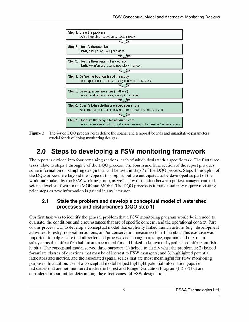
Figure 2 The 7-step DQO process helps define the spatial and temporal bounds and quantitative parameters
crucial for developing monitoring designs.
2.0 Steps to developing a FSW monitoring framework
The report is divided into four remaining sections, each of which deals with a specific task. The first three
tasks relate to steps 1 through 3 of the DQO process. The fourth and final section of the report provides
some information on sampling design that will be used in step 7 of the DQO process. Steps 4 through 6 of
the DQO process are beyond the scope of this report, but are anticipated to be developed as part of the
work undertaken by the FSW working group, as well as by discussion between policy/management and
science level staff within the MOE and MOFR. The DQO process is iterative and may require revisiting
prior steps as new information is gained in any later step.
2.1 State the problem and develop a conceptual model of watershed processes and disturbances (DQO step 1)
Our first task was to identify the general problem that a FSW monitoring program would be intended to
evaluate, the conditions and circumstances that are of specific concern, and the operational context. Part
of this process was to develop a conceptual model that explicitly linked human actions (e.g., development
activities, forestry, restoration actions, and/or conservation measures) to fish habitat. This exercise was
important to help ensure that all watershed processes occurring in upslope, riparian, and in-stream
subsystems that affect fish habitat are accounted for and linked to known or hypothesised effects on fish
habitat. The conceptual model served three purposes: 1) helped to clarify what the problem is; 2) helped
formulate classes of questions that may be of interest to FSW managers; and 3) highlighted potential
indicators and metrics, and the associated spatial scales that are most meaningful for FSW monitoring
purposes. In addition, use of a conceptual model helped highlight potential information gaps i.e.,
indicators that are not monitored under the Forest and Range Evaluation Program (FREP) but are
considered important for determining the effectiveness of FSW designation.

FSW Conceptual Model and Alternative Monitoring Designs
ESSA Technologies Ltd. .
4
2.2 Identify FSW monitoring questions (DQO step 2)
The second task was to formulate monitoring questions to be addressed by the FSW monitoring program.
Question identification and a process of question clarification are important because it focuses the search
for specific information needed to address the problem. Alternative actions that could be triggered as a
consequence of monitoring results for a given question were also considered as part of this task.
2.3 Identify inputs to the decision (DQO step 3)
Our third task was to identify inputs to the decision. We started with a review of FREP’s Stream and
Riparian Management Areas (see Tripp et al. 2008) and Water Quality (see Carson et al. 2008)
monitoring protocols to see what FREP indicators might be transferable to a monitoring framework
designed to track status/trends in FSW condition. In so doing, we identified gaps where no FREP
indicators are available or suitable (e.g., indicators for upslope processes). Assessing additional
monitoring protocols used in other jurisdictions that could potentially fill these gaps was the primary
focus of a supplement literature review. For this task, we reviewed published, grey, and web literature to
identify potential indicators and protocols not included in FREP, but which would be valuable to include
within a FSW monitoring framework. In addition, we conducted a preliminary review of the site selection
and data collection procedures within the Protocol for Evaluating the Condition of Streams and Riparian
Management Areas (Tripp et al. 2008), in order to assess the feasibility of employing these methods
within a FSW monitoring framework.
We focused our literature review in three areas: a) scientific documentation supporting the use of
indicators not captured by FREP, but which are known to be important for monitoring stream function
and fish habitat; b) remote sensing protocols and methods that could be used within a FSW framework to
inform various indicators (e.g., mass wasting events); and c) the effectiveness and reliability of rapid
bioassessment procedures for determining watershed function/status.
2.4 Describe alternative approach/design options for monitoring watersheds
As a final task, we reviewed the academic and grey literature and consulted experts in the field of
sampling design, to identify a subset of approaches that may be suitable for FSW monitoring objectives.
We briefly describe these alternatives, as well as their strengths and weakness. This task represented an
initial exploration of DQO Step 7 related monitoring design alternatives, but is a task which can only be
fully pursued when the required discussions required to inform DQO steps 4 to 6 have been completed.
3.0 Identify the problem and develop a conceptual model (DQO step 1)
3.1 The problem
The particular problem to be evaluated is described in the FSW monitoring charter (L. Reese-Hansen, BC
Ministry of Environment, pers. comm.). The charter states that watersheds with both high fish value and
watershed sensitivity are designated as FSW to conserve i) fish habitat, and ii) the natural function and
processes required to maintain fish habitat values now and in the future. A monitoring program is needed
to ensure that FSWs are indeed protecting fish habitat and the processes required to maintain it. The
agencies ultimately responsible for making decisions related to FSWs are the BC MOE and forest and

FSW Conceptual Model and Alternative Monitoring Designs
ESSA Technologies Ltd. .
5
range operators. BC MOE will be responsible for developing the technical design of a monitoring
program that addresses this problem; however, the final design will be contingent on the extent of
interagency cooperation between BC MOE and BC Ministry of Forests and Range (BC MOFR). Non-
technical issues that could impact the development of a FSW monitoring design are departmental funding
and capacity constraints and jurisdictional differences (i.e., may have different levels of collaboration
across forest districts which may lead to different levels of monitoring effort).
3.2 Linking ecological processes to fish habitat and stream function
Freshwater habitats for fish are the product of interactions among climate, hydrologic response of
watersheds, hillslope, and channel erosion processes (Swanston 1991). Coupled with the type and extent
of vegetative cover, watershed processes control streamflow, input of nutrients into the stream channel,
channel stability, and the development of fish habitat suitable for fish spawning, incubation, and rearing.
In the absence of major disturbances watershed processes produce small but continuous changes in the
environment (i.e., natural variability), making it difficult to evaluate whether environmental changes are a
consequence of natural or human activity (Swanston 1991).
The basic components of aquatic ecosystems that need to be considered when evaluating ecological
condition and stream function include basin geomorphology, hydrologic patterns, water quality, riparian
forest conditions, and aquatic habitat characteristics for a variety of aquatic organisms (Naiman et al.
1992). Ecologically healthy watersheds have lateral, vertical, and longitudinal connections between
ecosystem components which are spatially and temporally variable (Reeves et al. 2004). This variability
adds a substantial degree of complexity to the quantification of direct links between processes and stream
function, as well as to the development of standards and expectations for aquatic ecosystems condition.
Cause-and-effect linkages between watershed processes and physical and biological response are unique
to habitat types. In addition, different species of fish use different habitats and are sensitive to different
levels of stream function condition. Some of the cause-and-effect linkages between watershed processes
and fish habitat used by different life stages are illustrated in Figure 3 (Nelitz et al. 2007). Habitat
pressures at the watershed level (upslope subsystem) are represented by red boxes. Habitat pressures at
the stream level (riparian and floodplain and in-channel subsystems) are represented by white and light
grey boxes. Life stage response is represented by dark grey boxes. For example, water extraction
(watershed pressure) affects stream discharge (in-stream pressure) which can in turn affect adult spawners
via changes in the amount of viable spawning habitat. In addition, changes in stream discharge can affect
in-stream temperatures, which can affect the extent of suitable juvenile rearing and spawning habitat.

FSW Conceptual Model and Alternative Monitoring Designs
ESSA Technologies Ltd. .
6
Figure 3 Summary of linkages among upslope (red boxes), riparian floodplain (white or light grey boxes), and
stream (white or light grey boxes) pressures on fish habitat and life stage (dark grey boxes) (Modified
from Nelitz et al. 2007).
3.3 Conceptual model
To be meaningful, a monitoring program should provide insights into cause-and-effect relationships
between environmental stressors and anticipated ecosystem responses (Reeves et al. 2004). The first step

FSW Conceptual Model and Alternative Monitoring Designs
ESSA Technologies Ltd. .
7
in developing a monitoring plan is to identify the factors that influence the ecological processes of interest
and respective indicators. The high level conceptual model illustrated here, highlights the links between
fundamental watershed processes, natural and human caused stressors, and stream function and fish
habitat (Figure 4). The conceptual model also recognizes that watersheds vary regionally, and that this
variability plays an important role in determining the magnitude, frequency, and pathways of disturbances
in each of the three subsystems. Consequently, the model must account for the inherent watershed-scale
landscape characteristics of topography, geology, and climate when developing reliable indicators of
condition. The model highlights that watershed processes occurring in each of the subsystems (upslope,
riparian, and in-channel) has the potential to affect physical process, stream function, and fish habitat in
different ways. It is important to emphasise that the conceptual model presented here is a starting point
from which a more detailed and refined conceptual model should be developed. Creating a conceptual
model is not a one-off process, rather it is one that is repeated and refined a number of times during a
study as research questions become more specific, experts are consulted with, and hypotheses are tested
(Robinson 2006).
Figure 4 Overview diagram outlining the basic components of a watershed that need to be considered when
evaluating ecological condition, stream function, and fish habitat. Basic watershed components include
basin geomorphology, hydrologic patterns, water quality, riparian condition, and aquatic habitat
condition. All watershed components and processes are influenced by climate.
A conceptual model provides a perspective at the system scale of the linkages among physical, chemical,
and biological components and processes in an ecosystem (Nelitz et al. 2007). Such a perspective is
valuable for this work because it:

FSW Conceptual Model and Alternative Monitoring Designs
ESSA Technologies Ltd. .
8
1) provides a framework for summarising the current state of knowledge describing the key cause
effect linkages between watershed processes and stream function/fish habitat;
2) improves clarity and transparency for discussion around indicator selection for monitoring
purposes;
3) helps to ensure that selected indicators are responsive to environmental change be it human or
naturally induced; and
4) helps to ensure recommendations around monitoring design address the pressures on stream
function/fish habitat.
One of the key questions when trying to ascertain ecological condition is:
Are the key processes that create and maintain habitat conditions in aquatic and
riparian systems intact?
However, before addressing this question the key watershed processes need to be identified. We therefore
mapped out the key processes in each subsystem that affect stream function and fish habitat (Figure 5).
For instance, a watershed’s ability to effectively store and release water is critical for maintaining stream
function in a number of ways, some of which include: i) decrease effect of extreme flood events by
storing water in soils and plants; and ii) gradual release of water from soils and snowpack (Swanston
1991).
The processes occurring in the upslope subsystem (i.e., in the watershed in general) are assumed to affect
the riparian floodplain subsystem which in turn affects the stream channel subsystem. The riparian and
floodplain subsystem may to some extent buffer the effects of the upslope system on the stream channel
(degree of buffering is situation dependent) (Platts 1991). Stream channel and riparian floodplain
subsystems are intricately coupled so that changes in states or function associated with processes and
stressors in one subsystem generally affect the linked subsystem (Naiman et al. 1992). In contrast, the
influence of the riparian subsystem on the upslope subsystem is assumed to be nearly, but not completely,
negligible.

FSW Conceptual Model and Alternative Monitoring Designs
ESSA Technologies Ltd. .
9
Figure 5 Key processes affecting stream function and fish habitat are grouped according to the subsystem in
which they occur. The magnitude and frequency of processes in each subsystem are affected by climate.
Arrow size is representative of the degree to which processes in one subsystem affect processes in
another subsystem.
3.4 Stressors and influence on stream function and fish habitat
Major disturbance of watershed processes, be they human or natural in origin, can drastically alter habitat
condition and stream function. In brief, disturbances can result in movement and redistribution of
spawning gravel, addition of sediment and woody debris, changes in stream productivity, and changes in
accessibility to habitat. For example, an increased input of storm water can lead to channel erosion,
resulting in channel widening and sediment deposition downstream. An increase in sediment loads may in
turn alter the habitats of fish and/or the benthic macroinvertebrates on which they feed, resulting in a
change in stream condition and function. The actual effect of watershed processes, such as floods, on
habitat and stream function is largely dependent on the frequency and magnitude of the disrupting events.
Using the conceptual model and key processes by subsystem as a guide (Figures 4 and 5), we identified a
suite of stressors that are most likely to affect stream function and fish habitat across all types of
watersheds (Table 1). The stressors are intended to be value neutral, meaning they can either negatively
or positively impact stream function and fish habitat. For example, mass wasting events can have either

FSW Conceptual Model and Alternative Monitoring Designs
ESSA Technologies Ltd. .
10
negative or positive impacts depending on the quantity and size of sediment and woody debris added to
the system and the frequency at which events reoccur. For the sake of simplicity, stressors have been
stated in general terms. For example, change in vegetation cover is meant to encompass a variety of
potential stressors such as land use, timber harvest, forest/vegetation type, fire, insects and pathogens.
Stressors can be further refined when deciding on which indicators to use for monitoring FSW status.
Table 1 List of key processes intrinsic to stream function, the stressors affecting them, and the resulting affect on
stream function and fish habitat.
Component Key process Stressors* Influence to stream function and fish
habitat
Upslope subsystem
Hydrological Water storage and release Change in vegetation cover; roads; extreme climate events
Changes in runoff timing, magnitude, and water storage
Vegetation Wood production and transport
Change in vegetation cover Forest fragmentation, debris, nutrient cycling
Soil Sediment production and transport
Surface erosion, mass wasting; and roads
Nutrient cycling, soil moisture, formation rates, and sediment regime
Riparian floodplain subsystem
Hydrological Water storage and release Change in vegetation cover; roads; extreme climate events
Changes in runoff timing, magnitude, water temperature, and toxins
Hydrological Flood tolerance (i.e., soil erosion channel movement, bank erosion)
Change in riparian vegetation Changes in sediment load, bank stability, fish habitat availability
Vegetation Vegetative community structure; succession, growth, and mortality
Landscape disturbance Forest fragmentation, debris, nutrient cycling, and changes in microclimate
Vegetation LWD supply and retention Change in riparian vegetation Creation of stream channel fish habitat, refugia
Soil Sediment production and transport
Surface and bank erosion, mass wasting; roads
Nutrient cycling, soil moisture, formation rates, and sediment regime
Thermal energy transfer
Microclimate regulation Change in riparian vegetation Microclimate and water temperature
System productivity Chemical and nutrient delivery
Loss of riparian vegetation; changes in water quality
System productivity, available nutrients, toxins
Stream channel subsystem
Hydrological Flood tolerance (i.e., soil erosion, channel movement, bank erosion)
Change in vegetation cover; change in riparian vegetation
Habitat loss, channel scour and morphology,
Hydrological Water delivery (i.e., how and when water enters the system), flow, and yield
Landscape disturbance; in-stream barriers
Habitat loss, redd dewatering, spawning ground loss
Channel Structure Sediment delivery and habitat formation
Landscape disturbance; roads and road crossings; mass wasting
Habitat loss, change in stream channel form and sediment supply regime
Channel Structure LWD delivery and habitat formation
Change in vegetation cover; change in riparian vegetation
Change to fish habitat, channel form, refugia
Thermal energy transfer
Microclimate regulation Changes in riparian vegetation Microclimate and water temperature
System productivity Chemical and nutrient delivery
Loss of riparian vegetation; changes in water quality
Habitat loss, change in stream channel form and sediment supply regime
Identified stressors can act synergistically to produce cumulative watershed impacts (CWI), which are
defined as impacts that influence or are influenced by the flow of water through a watershed (Reid 2001).
CWIs include impacts that arise from either a single factor or any combination of factors, including,
changes in hydrology, erosion, in-stream woody debris, channel form, chemicals, heat, flora and fauna,

FSW Conceptual Model and Alternative Monitoring Designs
ESSA Technologies Ltd. .
11
and water quality (Reid 2004). The majority of impacts that occur away from the site where the triggering
land-use activity occurred are CWIs because something must be transported from the site of the activity to
the site being impacted (Reid 2001).
Thresholds are a commonly used method for preventing cumulative effects and have been discussed as a
possible tool for FSW monitoring as a means to decide when an undesirable effect (impact) has been
reached. However, a threshold approach has limited utility if the intent is to reverse existing or prevent
future cumulative effects because the majority of responses of interest significantly lag behind the land
use activities (Reid 2001). For example, aggradation at downstream sites (the result of elevated rates of
erosion from a site impacted by development), can take decades to manifest itself. If a threshold is
defined according to a system response, the trend of change may be irreversible by the time the threshold
is surpassed. It is therefore important to consider the rate with which a system responds to a specific
impact when deciding whether using thresholds is appropriate for the prevention of cumulative effects
from a specific impact and what the appropriate threshold level should be.
The past several decades have seen a growing emphasis on the need to evaluate and regulate cumulative
impacts; however, management of CWIs is one of the most difficult issues to deal with (Stein and
Ambrose 2001). This difficulty stems from the high degree of variability in how CWI manifest
themselves both spatially and temporally (Johnston 1994), e.g., distance from action. There is a general
lack of understanding of the spatial and temporal interactions of individual impacts and how they should
be monitored (Stein and Ambrose 2001). If CWI are to be avoided and managed for in any meaningful
way, managers must have a thorough understanding of the causal mechanisms between activity and
impact at appropriate temporal and spatial scale (Reid 2001; Stein and Ambrose 2001). That is, causal
mechanisms, symptoms, and impact persistence need to be determined and monitored at a broad enough
scale using landscape approaches that include enough area for the accumulation of impacts to be
recognised (Reid 2001). Identification and understanding of causal mechanisms makes it possible to take
a more proactive approach towards CWI management because the potential influence of planned
activities can be inferred and taken into account from the beginning of the planning process (Reid and
Furniss 1999; Reid 2001; Stein and Ambrose 2001). Watershed analysis will ideally described the most
important cause-and-effect linkages between land-use activity and system response in a particular are of
interest, such that individual activities known to cause an impact can be monitored and assessed based on
the scale of the activity taking place (Reid and Furniss 1999).
4.0 Candidate FSW questions (DQO step 2)
4.1 Question development
Questions can be developed in a number of ways. One possibility is to use the main monitoring questions
asked using the FREP sampling protocols (e.g., a total of 15 questions addressed in Tripp et al. (2008))
and evaluate them similarly for FSWs, but with the following overarching question in mind: Is it
necessary/desired to know this information in the particular form developed by FREP, or can/should the
information be expressed/used in a more general way?
Alternatively, monitoring questions can be developed by thinking about the reporting needs or treatment
effects, which may already be well defined in some cases. For example, in answering a question such as
“Are there significant differences between S3 and S4 streams in undisturbed versus disturbed watersheds
in the Interior of BC,” it might be sufficient to report out the distribution of final high-level FREP stream
assessments (Properly Function, Properly Functioning at risk, etc.) between the two treatments.

FSW Conceptual Model and Alternative Monitoring Designs
ESSA Technologies Ltd. .
12
Once a set of questions emerges, it will be necessary to consider how each question will be worked out in
terms their spatial and temporal bounds, necessary data inputs, the statistical design best suited to the
question, and reporting outputs. Answering the details around each question will help direct the sampling
and monitoring design.
4.2 Question clarification
It is important to provide decision-makers with information on why particular types of information are
important for quantitative design. Doing so provides a way of moving beyond a general discussion of
design considerations and helps avoid developing a design that provides a precise answer to the wrong
question. As a start to this process, it can be useful to adopt a “Question Clarification” process (see
CSMEP 2005). The “Question Clarification” process is designed to allow biologists / biometricians to
both inform decision-makers about the quantitative needs for monitoring design and to help extract this
information from them via a series of clarifying questions. While these questions address the same
information needs touched upon in Steps 1 to 7 of the DQO, they focus on more specific data needs and
address the implications for the design process when this is not provided. By moving through the
“Question Clarification” process, a decision-maker should be able to provide the information necessary to
develop monitoring questions that are consistent with policy and explicit enough to guide a biologist /
biometrician in the quantitative design of a monitoring program to address those questions.
Questions to be addressed through this process can be broken into 3 categories: management questions,
monitoring questions, and sampling questions. Answers to management questions will provide focus
about the desired state or condition of the resource, and provide a measure of management success. As
described by Elzinga et al. (2001), management questions can usually be classified in relation to two
types of objectives: (1) target/threshold objectives, and (2) change/trend objectives. Answers to
monitoring questions provide additional detail about what the monitoring program will do. A long term
monitoring program needs to focus on a set of objectives that meet the test of being realistic, specific, and
measurable. Answers to monitoring questions should allow the analyst to anticipate what the required
data will look like, and should have a good sense of what potential measures will or will not be included
for monitoring. Monitoring questions also help clarify what the sampling protocols should do, and help
place boundaries and limits on what will be included in the monitoring by specifying particular study
areas, species, or measures. Answers to sampling questions focus on statistical objectives and clarify
specific information needs such as required levels of precision, power, acceptable Type I and II error
rates, and the magnitude of change you are hoping to detect. An example of a sampling objective would
be as follows: We want to be 90% certain of detecting a 40% change in habitat condition and we are
willing to accept a 10% chance of saying a change took place when it really did not.
Based on our discussion with individuals involved in the development of the FSW monitoring program,
we have concluded that the FSW program is presently at the stage of defining management questions that
focus on target/threshold objectives and change/trend objectives. Specific targets/thresholds for watershed
processes of interest that will be used to determine watershed status remain to be defined. As the
management questions are further refined, the monitoring (part of DQO steps 2 and 4) and sampling
questions (DQO step 5 and 6) associated with each will begin to form.
4.3 Candidate questions
There are three tiers of management questions that could inform the decision making process for FSWs
management. Each tier refers to a particular scale of interest, and will in turn dictate the type of

FSW Conceptual Model and Alternative Monitoring Designs
ESSA Technologies Ltd. .
13
monitoring framework needed depending on which of the questions are selected. The first tier of
management questions examines FSWs as a class of actions:
How do FSWs perform as a ‘class’ of actions, i.e., in general how are FSWs doing
relative to non-FSWs (e.g., proportion of functioning watersheds to non-functioning
within each class of actions)?
More specific monitoring questions relating to this tier can be asked in conjunction with this broad-scale
question. For example, it may be of interest to know how FSWs compare to non-FSWs with respect to a
specific indicator:
How do FSW perform relative to non-FSWs with respect to LWD processes, mass
wasting events, or vegetation cover?
Development of monitoring questions will require that specific indicators be chosen which will act as the
basis for comparing FSWs to non-FSWs. The FSW program may decide that several indicators should be
used to answer the first tier management question, in which case data aggregation methods will need to be
chosen and tested (DQO step 4; refer to Appendix B for a discussion of possible data aggregation
methods) . The desired level of precision to detect whether a difference exists and/or whether a threshold
has been exceeded remains to be defined (sampling question). An initial starting point for a sampling
question at this tier may be:
We want to be 80% certain of detecting a difference between FSWs and non-FSWs and
we are willing to accept a 20% chance of saying a difference exists when it really does
not.
The feasibility of being able to answer the above stated management question with this degree of
precision will have to be assessed taking into account several factors including: the resources available to
the FSW monitoring program and the degree of certainty needed for management decision. Refer to
Appendix C for a lengthier discussion on the specification of tolerance limits.
The second tier of management questions focuses exclusively on FSWs and examines the differences
between FSWs that are considered to be functional (green) versus those that are not functional (red):
What is the difference between watershed processes in functional vs. non-functional
FSWs (i.e., what is causing FSWs to be non-functional)?
Investigation at this scale serves two functions. First, detailed monitoring will provide insight into what
key watershed processes have failed, thus causing the observed outcome of non-functional. Information
on the cause of failure can in turn be used to make statements about the status of non-functional FSWs.
An example statement is: 60% of FSWs are scored as non-functional because of excessive mass wasting
events. Second, data collected from monitoring of functional and non-functional watersheds can be used
to refine threshold criteria for defining functional vs. non-functional for all indicators. This information
can then be used to inform both Tier 1 and Tier 2 management questions.
The third tier of management question deals with FSWs at the individual scale:
Are habitat protection objectives for a particular FSW being maintained (e.g., in
relation to targets for specific habitat indicators within a FSW)?
FSW Conceptual Model and Alternative Monitoring Designs
ESSA Technologies Ltd. .
14
The intention of management questions at the individual scale is to determine whether improvement in
the status of individual FSWs has taken place as a result of particular actions. The nature of the
monitoring questions at this scale will be dependent on which watershed processes were identified as
failing in response to the Tier 2 management question. The desired level of precision to detect a change in
condition remains to be defined (sampling question).
5.0 Identify data inputs into the decision (DQO step 3)
Once the candidate questions have been specified the next step is to identify the information required (i.e.,
indicators / performance measures (PM)) to answer management and monitoring questions and to identify
what data could be used to inform the PMs. The PMs selected to address each question will be contingent
on input data and the conceptual model outlining system interactions of interest. The reporting needs for
each candidate question may vary; consequently the methods used to meet these needs may take on
several different forms depending on the question. For example, it might be necessary to produce a
summary of trends in stream health given a variety of strata and treatments to answer one specific
management question, while another might only require statements about significant changes (or absence
of significant changes).
In order to move towards greater harmonisation of monitoring across the province and to leverage past
efforts, one of the primary data inputs into the decisions for the FSW monitoring program will be
performance measures collected using FREP protocols (see Section 5.3). Data inputs not captured by
FREP, but which may be important inputs into the decision making process are discussed in Section 5.4
and 5.5. A candidate list of indicators/metrics to inform the questions should be compiled based on
Tables 2 and 3, and potential confounding factors should be identified. The final selection of data inputs
and indicators will also be informed by data availability, data aggregation method, and necessary
precision.
5.1 FREP background
In 2004, FRPA came into effect introducing the regulatory framework that would transition BC to a
results-based forest management approach. Under the results based approach to forest management, the
forest industry is responsible for developing results and strategies, or using specified defaults, for the
sustainable management of resources (BC MOFR 2007). The role of government is to ensure compliance
with established results and strategies, and evaluate the effectiveness of forest and range practices in
achieving management objectives (BC MOFR 2007). Effectiveness monitoring under FRPA is carried out
by FREP, a multi-agency program established by government, to ensure that the stewardship of the eleven
resource values identified under FRPA is achieved. Rapid biological assessment (RBA) protocols and
appropriate indicators for each of the eleven resource values have been developed under FREP to monitor
resource values. RBAs are defined as cost effective assessments that use semi-quantitative methods to
quickly collect, compile, analyze, and interpret environmental data to facilitate management decisions and
resultant actions for control and/or mitigation of impairment (Barbour et al. 1999). Knowledge gained
through watershed research provides the scientific foundation for evaluating the effectiveness of forest
practices.
5.2 Rapid biological assessment (RBA) protocols
Rapid biological assessment (RBA) protocols to determine ecosystem function and biotic integrity of
watersheds have become an important component of aquatic systems management (Utrup and Fisher

FSW Conceptual Model and Alternative Monitoring Designs
ESSA Technologies Ltd. .
15
2006; Marchant et al. 2006). RBAs have grown in popularity over the past decade because they avoid the
time consuming quantitative elements of traditional biological assessment methods and satisfy the
demand for cost effective and timely monitoring (Growns et al. 1997; Fennessy et al. 2007). Another
advantage of using RBA methods is that they can be used to validate and refine landscape level
assessments and techniques (Fennessy et al. 2004). RBA methods are currently used in Europe by the
European Water Framework Directive to provide a basis for management, in Australia to guide water
management, and in the USA for purposes as diverse as ranking wetlands for protection (see Collins et al.
2007), the regulation of water quality, invasive species management, and fire regime mapping (see TNC
2008).
RBA have been criticized on several levels. First, RBAs that focus exclusively on biological components
do not provide accurate information about species abundance, consequently it is assumed that RBAs can
only detect gross impacts and that they are not as sensitive as quantitative methods (e.g., Taylor 1997).
The FREP protocol utilizes a suite of over 50 indicators thus allowing it to examine both biological and
physical components of stream/riparian ecosystem. Second, there is the possibility for inter-operator
differences, where sampling undertaken by community groups, volunteers, or other individuals with little
experience or formal training can produce substantially different results from trained field technicians
(Metzeling et al. 2003; Navies and Gillies 2001). Engel and Voshell (2002) demonstrate that iterative
refinement of RBA protocols to ensure inter-operator consistency can minimize the effect of operator
variability such that conclusions on ecological function reached by volunteer oriented protocols and
professional oriented protocols are similar. Last, choosing appropriate reference sites is often problematic,
where the ability of RBAs to detect ecological condition is dependent on the reference sites selected
(Turak et al. 1999).
Comparisons of RBA protocols used by FREP and more traditional quantitative protocols have shown
that RBAs are effective at detecting declines in overall stream/riparian health (Peter Tschaplinski, BC
Ministry of Forests and Range, pers. comm.). A rapid assessment of rivers using macroinvertebrates
yields similar conclusions on the effectiveness of RBA for detecting change (see Metzeling et al. 2003;
Sloan and Norris 2003).
Fennessy et al. (2007) identified five general areas that need to be addressed when adapting existing
methods or developing RBA methods to assess condition:
1) definition of the assessment area;
2) treatment of site type;
3) methods for scoring;
4) consideration of highly valued stream types or features; and
5) procedures for validation with comprehensive ecological data so that the rapid method can be
used to extrapolate more detailed results to the resource base as a whole.
Consideration of each element highlighted by Fennessy et al. (2007) in the development of a FSW
monitoring framework will help ensure successful detection of site degradation.

FSW Conceptual Model and Alternative Monitoring Designs
ESSA Technologies Ltd. .
16
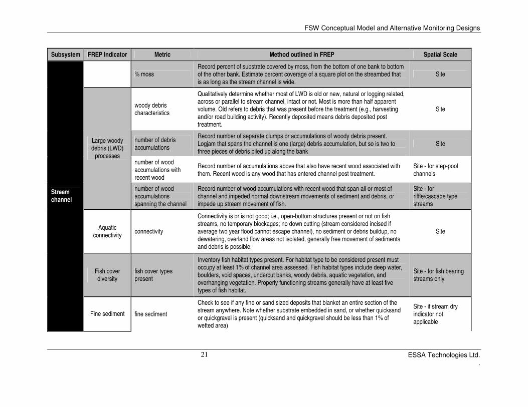
5.3 Summary of FREP’s relevant indicators for FSW monitoring
Currently, two FREP protocols are relevant for FSW purposes: streams and management riparian areas
and water quality. Additional FREP protocols for windthrow, fish passage, and mass wasting are being
developed and will be useful to the FSW monitoring program. The FSW monitoring initiative would
benefit from incorporating the data collection methodology already established under FREP for these two
relevant resources values, as well as those mentioned which are being developed. The benefit of using
FREP protocols is twofold: 1) data compatibility across sites that are monitored under different programs;
2) efficiencies in cost of program development and personnel training; and 3) comparison between FSWs
and non-FSWs across the province. Indicators, metrics, and collection methods described for the resource
values fish/riparian and water that may be useful for monitoring FSW stream function and habitat status
are listed in Table 2.

FSW Conceptual Model and Alternative Monitoring Designs
ESSA Technologies Ltd. .
17
Table 2 Summary of FREP indicators and methods of data collection taken from the protocols for water quality and streams and riparian management areas.
Subsystem FREP Indicator Metric Method outlined in FREP Spatial Scale
Upslope None
mid-channel bars (m)
Mid-channel bars, diagonal bars, spanning bars, and braided bars should all be treated as mid-channel bars. Use a hand-held tape or hip chain to directly measure the length of reach with the bar types, or visually estimate length in short manageable sections of known length. Where same type of gravel bars overlap do not measure overlap twice
Site
lateral bars (m) Measure as per mid-channel bars and wedges. Site
Channel bed disturbance
multiple channels and braids (m)
Includes any active channel that is separated by an island (vegetated or gravel) and dry side channels separated by vegetated islands. Record reach length where multiple channels and braids are present
Site
length of stream with deeply rooted vegetation (m)
Measure length of stream on both sides of the stream reach. Consider only the vegetation within first 1m of the rooted edge.
Site
length of stream reach with recently disturbed bank (m)
Measure total length of indicator on both banks even if management activity being assessed only occurs on one side (do not double count stream length if metric on one bank overlaps with same metric on the other bank). Non-erodible boulder or bedrock not to included.
Site
length of stream reach with recently upturned root wads (m)
Measure total length of indicator on both banks even if management activity being assessed only occurs on one side (do not double count stream length if metric on one bank overlaps with same metric on the other bank). Measure length of each root wad from the upstream edge to the downstream edge.
Site
non-erodible banks (m)
Record the reach length where naturally non-erodible banks are present on both sides of the stream. Subtract reach length with naturally non-erodible banks on both sides from total reach length to give total “erodible” reach length.
Riparian Floodplain
Channel bank disturbance
length of stream with stable undercut banks (m)
This metric not relevant for non-alluvial channels. Measure total length of indicator on both banks even if management activity being assessed only occurs on one side (do not double count stream length if metric on one bank overlaps with same metric on the other bank). Non-erodible boulder or bedrock not to included. Bank considered to be undercut when depth is at least 2% of channel width and height is at least within two times this distance.
Site

FSW Conceptual Model and Alternative Monitoring Designs
ESSA Technologies Ltd. .
18
Subsystem FREP Indicator Metric Method outlined in FREP Spatial Scale
LWD supply adequate LWD supply retained
Using stream classification and retention levels recommended in Riparian Area Management Guidebook determine if adequate LWD supply in first 10m
Site
bare soils in first 10m (m2)
Locate and visually estimate the area of each patch of bare ground present in the first 10m of the riparian area, including all permanently deactivated or de-built roads. Where bare ground not present as discreet bare patches that can be measured individually, but is dispersed throughout the vegetation, use the percent cover class card to estimate the amount of bare ground. Bare soils and bare erodible ground are the same thing.
Site
bare soils exposed to rain in first 10m (m2)
For each patch of bare ground recorded within first 10m, record what area is outside of the drip line and therefore directly exposed to rainfall.
Site
bare soil hydrologically connected to first 10m (m2) plus bare soil in first 10m (m2)
Look at all active roads within first 10m of riparian are plus all other ground beyond the first 10m. Treat any seasonally or temporally deactivated roads as active roads. Bare ground outside first 10m could include any other eroded surfaces, cut/fill slopes, failures, sloughs, slides, or torrents that may be far from riparian area but nevertheless hydrologically connected either by ditch lines, slide tracks, or stream channels.
Site
disturbed ground in first 10m (m2)
Disturbed ground is affected by pugging, hummocking, or rutting, usually by animals or vehicles. Main characteristic of concern is soil compaction. Locate and measure the area of all disturbed ground present in the first 10 m of the riparian area, including all permanently deactivated or de-built roads.
Site
Riparian soil disturbance
disturbed ground hydrologically connected to first 10m (m2) plus bare soil in first 10m (m2)
Look at all active, seasonally deactived or temporarily deactivated roads in the first 10 m of the riparian area plus all other disturbed ground beyond the first 10 m that may be hydrologically connected to the first 10 m
Site
extent of browsing/grazing
Heavily browsed shrubs are or are not present. Heavy grazing is or is not present on more than 10% of available forage
Site
riparian structure Does the distribution and relative abundance of the vegetation layers and forest components present collectively approach 75% of what is expected at similar but otherwise healthy, unmanaged sites in your area
Site
Riparian Floodplain
Vegetation form, vigour,
and recruitment
form Is form normal or not, vigour normal or not, recruitment normal or not Site

FSW Conceptual Model and Alternative Monitoring Designs
ESSA Technologies Ltd. .
19
Subsystem FREP Indicator Metric Method outlined in FREP Spatial Scale
presence of moisture loving plants
Are moisture loving plants present or not, if present are they healthy or no. Species include: willows, rushes, reeds, speckled alder, salmonberry, Devil's club, horsetails, ferns, mosses, liverworts.
Site
bank soil Are bank soils cool or warm, moist or dry, unchanged or not Site
Shade and bank microclimate
% shade
Percent shade at any point is the average of the two shadiest of east, west, or south aspects. Measure shade at a 60-degree angle above the horizontal. Looking through a circle made by your thumb and forefinger and held straight out above your head at a 60-degree angle to the E, S, and W is a useful area upon which to base visual estimates. For small streams < 2 m wide, shade can be estimated from the center of the channel. For wider streams, estimate shade on both sides of the streams and record the average of those two estimates.
Site
% disturbance increaser species
Record what % of a 10m transect is occupied by disturbance increaser plants within first 10m of riparian area. Transect should be perpendicular to stream reach
Site Disturbance
increaser plants
% noxious weeds Record what % of 10m transect is occupied by noxious weeds and/or invasive plants in first 10m. Transects should be perpendicular to stream reach.
Site
recent windthrow (number)
Count the number of recent (i.e., post-harvest) windthrown trees present in the designated management area. Compare this number with the number of standing trees below to estimate % windthrow. If number of windthrows or the number of trees present is too difficult to count, sub-sample the riparian area with fixed area plots to estimate total number of trees or windthrows present. With experience in assessing percent windthrow, a simple visual estimate of percent windthrow is appropriate if the percent of trees windthrown is clearly much greater than 10% of the trees, or less than 1%. % New = (# New) / (# Standing+ # New) X 100
Riparian Floodplain
old windthrow (number)
Count number of old (i.e., pre-harvest) windthrown trees present if it looks like the amount of old windthrow needs to be accounted for in assessing significance of recent windthrow.
Windthrow frequency
standing trees (number)
Count number of standing trees if percent of trees windthrown could be between 1 and 10% of all stems, or where you lack confidence in estimating percent windthrown. Rough estimates are appropriate if % windthrown < 1 or > 10. % Old = (# Old) / (# Standing+ # Old + # New) x 100
Site - In a RMA, if a reserve is present, the entire reserve or wildlife patch should be assessed. Also check adjacent management zone if trees were retained. If there is no reserve or wildlife tree patch, entire management zone should be assessed, provided some retention was prescribed

FSW Conceptual Model and Alternative Monitoring Designs
ESSA Technologies Ltd. .
20
Subsystem FREP Indicator Metric Method outlined in FREP Spatial Scale
volume of fine sediment lost by surface erosion
Estimate depth of annual erosion from road surface as a function of slope and road quality and multiply by the area experiencing to erosion. For surfaces associated with mini-catchments depth of annual erosion is a function of ground cover and surface type and multiply by the area experiencing to erosion.
Site
Riparian Floodplain
Sediment volumes at
stream crossings volume of fine
sediment lost by mass wasting
Estimate length, width, and depth of landslide scares, gullies, or rills to get an estimate of volume eroded from the site. Multiply estimated volume by estimate of portion of fine sand, silt, and clay eroded (excludes active roads). Estimate of portion of fines calculated using hand texturing or jar technique. Only consider if mass wasting contribution > 0.5m3.
Site
species richness List all different invertebrates sampled Site - minimum of six stations should sampled at a site
number sensitive invertebrate types
Sample benthic inverts at each sample station with dip net using white tray to sort through the sample. Sensitive species include mayflies, caddisflies or "case-builders", stoneflies, riffle beetles, "hellgrammites", clams.
Site - minimum of six stations should sampled at a site
number of major invertebrate groups
Record number of major invertebrate groups present in each sample. Major groups includes: insects, mites, worms, molluscs, and crustaceans.
Site - minimum of six stations should sampled at a site
Aquatic invertebrate
diversity
number of insect types Record number of insects present at each sample station Site - minimum of six stations should sampled at a site
moss condition Qualitative observation of moss condition. Is moss intact and vigorous or is it dead, desiccated, scoured, or buried.
Site
Stream channel
Moss abundance and
condition
moss (m)
On non-alluvial streams, record the length of stream reach that has some moss at some point, regardless of its overall abundance. Not an area measurement of moss abundance like the measurement made for moss at the point samples. It is a linear measurement of moss presence only along the entire length of the sample reach.
Site
FSW Conceptual Model and Alternative Monitoring Designs
ESSA Technologies Ltd. .
21
Subsystem FREP Indicator Metric Method outlined in FREP Spatial Scale
% moss Record percent of substrate covered by moss, from the bottom of one bank to bottom of the other bank. Estimate percent coverage of a square plot on the streambed that is as long as the stream channel is wide.
Site
woody debris characteristics
Qualitatively determine whether most of LWD is old or new, natural or logging related, across or parallel to stream channel, intact or not. Most is more than half apparent volume. Old refers to debris that was present before the treatment (e.g., harvesting and/or road building activity). Recently deposited means debris deposited post treatment.
Site
number of debris accumulations
Record number of separate clumps or accumulations of woody debris present. Logjam that spans the channel is one (large) debris accumulation, but so is two to three pieces of debris piled up along the bank
Site
number of wood accumulations with recent wood
Record number of accumulations above that also have recent wood associated with them. Recent wood is any wood that has entered channel post treatment.
Site - for step-pool channels
Large woody debris (LWD)
processes
number of wood accumulations spanning the channel
Record number of wood accumulations with recent wood that span all or most of channel and impeded normal downstream movements of sediment and debris, or impede up stream movement of fish.
Site - for riffle/cascade type streams
Aquatic connectivity
connectivity
Connectivity is or is not good; i.e., open-bottom structures present or not on fish streams, no temporary blockages; no down cutting (stream considered incised if average two year flood cannot escape channel), no sediment or debris buildup, no dewatering, overland flow areas not isolated, generally free movement of sediments and debris is possible.
Site
Fish cover diversity
fish cover types present
Inventory fish habitat types present. For habitat type to be considered present must occupy at least 1% of channel area assessed. Fish habitat types include deep water, boulders, void spaces, undercut banks, woody debris, aquatic vegetation, and overhanging vegetation. Properly functioning streams generally have at least five types of fish habitat.
Site - for fish bearing streams only
Stream channel
Fine sediment fine sediment
Check to see if any fine or sand sized deposits that blanket an entire section of the stream anywhere. Note whether substrate embedded in sand, or whether quicksand or quickgravel is present (quicksand and quickgravel should be less than 1% of wetted area)
Site - if stream dry indicator not applicable
FSW Conceptual Model and Alternative Monitoring Designs
ESSA Technologies Ltd. .
22
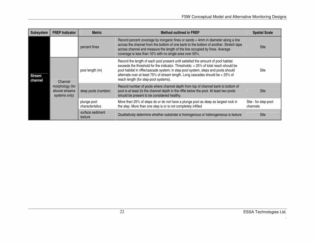
Subsystem FREP Indicator Metric Method outlined in FREP Spatial Scale
percent fines
Record percent coverage by inorganic fines or sands < 4mm in diameter along a line across the channel from the bottom of one bank to the bottom of another. Stretch tape across channel and measure the length of the line occupied by fines. Average coverage is less than 10% with no single area over 50%.
Site
pool length (m)
Record the length of each pool present until satisfied the amount of pool habitat exceeds the threshold for the indicator. Thresholds: > 25% of total reach should be pool habitat in riffle/cascade system; in step-pool system, steps and pools should alternate over at least 75% of stream length. Long cascades should be < 25% of reach length (for step-pool systems).
Site
deep pools (number) Record number of pools where channel depth from top of channel bank to bottom of pool is at least 2x the channel depth in the riffle below the pool. At least two pools should be present to be considered healthy.
Site
plunge pool characteristics
More than 25% of steps do or do not have a plunge pool as deep as largest rock in the step. More than one step is or is not completely infilled
Site - for step-pool channels
Stream channel Channel
morphology (for alluvial streams systems only)
surface sediment texture
Qualitatively determine whether substrate is homogenous or heterogeneous is texture Site

FSW Conceptual Model and Alternative Monitoring Designs
ESSA Technologies Ltd. .
23
5.4 Gaps identified in FREP and missing indicators
FSW monitoring is intended to provide data that will enable managers to determine the status of the
watershed, stream conditions, and fish habitat quality. Based on the focus and intention of FSW
monitoring, several gaps have been identified in the list of indicators monitored by the FREP for water
quality and streams and riparian management areas. For example drawing conclusions on watershed
status requires information on upslope areas (Reeves et al. 2004) and FREP protocols do not included
upslope indicators. The FREP water quality protocol does collect some information on mass wasting
(Carson et al. 2008).; however it primarily focuses on mass wasting events as they relate to roads and
therefore does not adequately capture other factors contributing to mass wasting events Indicator gaps,
additional metrics, and example protocols for data collection are listed in Table 3.
Upslope indicators such as vegetation composition and seral stage, roads, and land use are important to
capture because they reflect processes that influence the entire stream network within a watershed and are
relevant across the entire watershed (Naiman et al. 1992). Data for these indicators can be predominantly
gathered using remote sensing methods and analysis (see Section 5.5 for a description of remote sensing
protocols). Normalised Difference Vegetation Index (NDVI) is one indicator obtained via remote sensing
that has shown promise for detecting watershed changes. NDVI has been found to be closely correlated
with water quality parameters, and to a lesser extent with landcover proportions (Borstad et al. 2007).
This has the potential to be particularly useful for large-scale monitoring programs that would like to use
water quality as an indicator but do not have the resources to do so. Seasonal weather patterns, logging,
and man-made patterns and processes can also be detected in watersheds at many scales using changes in
NDVI (Borstad et al. 2007). There is also a possibility that NDVI could be used to measure riparian
condition, however, the 1 km resolution of NDVI may limit its ability to actually distinguish riparian
vegetation from surrounding vegetation.
Landscape change associated with urbanization, forestry, and agriculture poses major challenges to
aquatic ecosystems (Alberti et al. 2007). Effects of these changes on stream ecosystems include
simplification of stream channel structure through losses of large wood and channel straightening (Bilby
and Bisson 1998), decreased ability for a watershed to buffer against atmospheric pressures (Poole and
Berman 2001), changes in in-stream flow patterns (Sedell et al. 1990), and increased input of fine
sediment to streams from erosion and mass wasting events (Chamberlin et al. 1991). Several studies have
shown that the composition of land cover within a watershed can account for much of the variability in
water quality and stream ecological conditions (Grant et al. 1986; Fausch and Northcote 1992; Whistler
1996; Griffith et al. 2002), making land use and disturbance a valuable indicator for monitoring watershed
status and stream function. However, thresholds for land use types are extremely difficult to identify
because there is not a linear relationship between land use types and deleterious effects on salmon (Mike
Bradford, Fisheries and Oceans Canada, pers. comm.). Noteworthy is the study by Alberti et al. (2007)
which hypothesizes that multiple measures of landscape disturbance (land cover composition,
configuration, and connectivity of impervious area) affect the biophysical environment. A watershed
disturbance index integrating multiple habitat indicators may be the most simple and informative way of
accounting for several human disturbances (riparian disturbance, road development, impervious surfaces,
and land use cover). Fore (2003) notes that integrated measures of disturbance were better predictors of
biological responses than a single measure of disturbance. In other words, there were many correlations
among different disturbance metrics.
The construction and presence of roads can result in stream fragmentation and obstruction of fish habitat
(e.g., Park et al. 2008), increased sediment load in-stream (Chamberlin et al. 1991), and degradation of
spawning habitat (Furniss et al. 1991). The road metrics listed in Table 3 can be calculated with data
FSW Conceptual Model and Alternative Monitoring Designs
ESSA Technologies Ltd. .
24
sources available for BC (e.g., Watershed Statistics and National Road Network), and have been
commonly applied in other studies (e.g., MacCaffery et al. 2007; Angermeier et al. 2004). We recognize
that road density and road-stream crossing density may be correlated, but we include both because each
relates differently to impacts on salmon habitats. When calculating a road density metric, it is generally
recognized as important to distinguish between paved, unpaved, and deactivated roads (each affect
habitats differently). NCASI (2001) recommends further research around developing indices of road
disturbance and targets for management. Gucinski et al. (2001) provides a good technical synthesis about
the effects of roads on fish habitat, while also recommending further work around developing
benchmarks.
The distribution and health of native fish populations are strongly tied to temperature conditions in their
habitats (Brannon et al. 2004). Temperature may directly affect fish species in obvious ways, or indirectly
through interaction with other important variables. For example, given sufficient magnitude and time,
high temperatures can cause weight loss, disease, competitive displacement by species better adapted to
the prevailing temperature, or death (Sullivan et al. 2000). Forest harvesting can cause mean monthly
maximum stream temperatures to increase by as much as 8°C and mean annual maxima to rise 15°C
(Brown and Krygier 1970) in circumstances where specific stream and watershed condition determine the
extent of temperature increases. In the Pacific Northwest, timber harvest is known to increase peak stream
temperatures to 24◦C or higher (Bury 2004), which has the potential to negatively impact cold-water
stream fish species, as well as multiple other species in aquatic systems. For example, anadromous
species (e.g., chinook, coho, pink, sockeye, chum, and steelhead) and many resident species (e.g.,
kokanee, rainbow trout, mountain white fish) are intolerant to temperatures > 20°C and exhibit high rates
of mortality when temperatures reach levels >24°C (Oliver and Fidler 2001). Bull trout is particularly
sensitive to temperatures, where temperatures > 15°C are known to be lethal (Oliver and Fidler 2001).
Adequate water quality is important to fish throughout all life-history stages. Water quality determines
stream productivity and effects specific carrying capacity characteristics of streams. For example, nutrient
availability, particularly nitrogen and phosphorus, is a major factor regulating aquatic ecosystem structure
and productivity (Wigington et al. 2003). Increased abundance of stream algae leads to increased
abundance of stream herbivores and this increased productivity is carried through the aquatic community
to higher trophic levels, including fish (Bjornn and Reiser 1991). In recent years, researchers have
recognized the existence of oligotrophication, where humans have reduced the natural processes of
nutrient delivery to aquatic ecosystems in some areas of the Pacific Northwest (Stockner et al. 2000). This
phenomenon is in strong contrast to the more commonly recognized eutrophication in areas where
human-accelerated nutrient loading has stimulated the productivity of many aquatic ecosystems. One such
example of oligotrophication has been the decline in allochthonous organic matter into streams.
Allochthonous organic material is delivered into streams via four main pathways: streamside vegetation;
groundwater seepage; soil erosion; and fluvial transport from upstream (Murphy and Meehan 1991). A
decrease in the expanse of forests and vegetation within a watershed (both in the riparian and upslope
areas) can lead to a decrease in sources of allochthonous organic mater such as deciduous leaves, conifer
needles, and woody debris. In addition, adult salmon provide an important marine nutrient subsidy to
freshwater and terrestrial environments (Gende et al. 2002); therefore, nitrogen and phosphorous
concentrations will be important to monitor so as to understand the relative importance of salmon
carcasses in these environments and ensure that sufficient salmon escapement targets for the watershed
are met. Dissolved oxygen is also critical to the survival and development of eggs and juveniles (Bjornn
and Reiser 1991) and is valuable metric of water quality. The concentration of dissolved oxygen in a
stream is dependent on water temperature, consequently it may be sufficient to measure only one variable.

FSW Conceptual Model and Alternative Monitoring Designs
ESSA Technologies Ltd. .
25
Table 3 Summary of select indicators that may address gaps in FREP methodology or scope, taken from AREMP and PIBO protocols, BC Watershed
Assessment Procedures, and other grey and peer review documents.
Subsystem Indicator Protocol Metric Method Spatial Scale
Wilford 2003;
Millard et al. 2006
Number of fans by geomorphic process type and power
Using aerial photographs, classify fans by the most powerful type of geomorphic process that occurs on a fan: debris flow > debris flood > water flood. Four power levels are defined on the basis of the extent of forest disturbance: 1. No power describes situations where no evidence can be found of geomorphic processes having occurred in the past 250 years (approximately). 2. Low power events do not have sufficient power to uproot or break trees. Deposition of sediment occurs around trees. These events are not observable on 1:20,000 aerial photographs. 3. High power, site level events create narrow swaths through the forest on a fan. The width of these swaths is <20 m, and they are generally not visible on 1:20,000 aerial photographs. 4. High power, stand level events create swaths >20 m wide through the forest, visible on 1:20,000 aerial photographs.
Watershed
Rollerson et al.
2002
Landslide frequency (number of natural landslides >500 m2 in slope
area; number of minor natural landslides <500 m2 in slope area)
Analysis of aerial photographs (1:20,000 ) by a trained geologist. Photographs can be taken every year, five years, or ten years. Temporal scale will be dependent on monitoring needs.
Watershed
Upslope
Mass wasting and landslides
Millard et al. 2006; Rollerson et al.
2002 Landslide density
Analysis of aerial photographs (1:20,000 ) by a trained geologist. Photographs can be taken every year, five years, or ten years. Temporal scale will be dependent on monitoring needs.
Watershed
Land use and
alteration Alberti et al. 2007
Percent land (PLAND): sum of the area of all patches of a particular type divided by total area of the basin. Alternatively, could group land uses / patch types using more meaningful classes that more strongly link to watershed-stream processes affecting salmon (e.g., % impervious area, % semi-impervious, % forested, % grass, % exposed).
Satellite imagery combined with GIS could be used to classify land alteration and area. Land alterations could include: agriculture, urban development, harvested, burned diseased, mining, rangeland, landslides (i.e., exposed soil), undisturbed ecosystem type.
Watershed

FSW Conceptual Model and Alternative Monitoring Designs
ESSA Technologies Ltd. .
26
Subsystem Indicator Protocol Metric Method Spatial Scale
Land use and alteration
BC Watershed Assessment Procedure
Equivalent clear cut area (ECA): area harvested, decimated by pathogens/pests, or burned with consideration given to silivicultural system, regeneration, and location (i.e., elevation) of disturbance within watershed
Satellite imagery combined with GIS could be used to determine ECA.
Watershed
AREMP Area covered by vegetation type and seral stage
Upslope vegetation (all vegetation > 100 m from the stream channel) and riparian vegetation data (all vegetation < 100 m from the stream channel) were collected from the vegetation layer developed by the Interagency Vegetation Mapping Project (IVMP) in Oregon and Washington, and the CalVeg layer developed in California. Both layers were constructed using Landsat Thematic Mapper remote sensing data. Vegetation was classified into the following categories: Non-Forested/Grass-Forb - Deciduous - Stands composed of > 90 % deciduous species. Mixed - Stands that contain both conifer and hardwood species. Conifer – Stands composed of at least 90% coniferous species. Conifers in both pure and mixed stands were classified by seral stage using the following definitions: Early Seral - recent clear cuts to stands with trees less than 25 cm (10 in) diameter at breast height (dbh). Approximate stand ages from 0 to 24 years old. Mid Seral - Stands trees from 26 cm to 52 cm (10 - 20 in) dbh. Approximate stand ages from 24 to 80 years old. Late Seral - Stands with trees greater than 53 cm (20 in) dbh. Approximate stand ages >80 years old.
Watershed
Upslope
Vegetation seral stage and series
Borstad et al. 2007
Normalised Difference Vegetation Index (NDVI)
NDVI is a common indicator measuring the ‘greenness’ of land vegetation and ground cover. NDVI is a compilation of 5 terabytes of daily, 1km resolution weather satellite data. The data has been composited to 10 day periods to reduce data volume and cloud effect. More than 700 NDVI measurements provide a nearly continuous time series of chlorophyll-containing vegetation for all watersheds relevant to Pacific salmon for the past 22 years (1985 to 2006)
Watershed
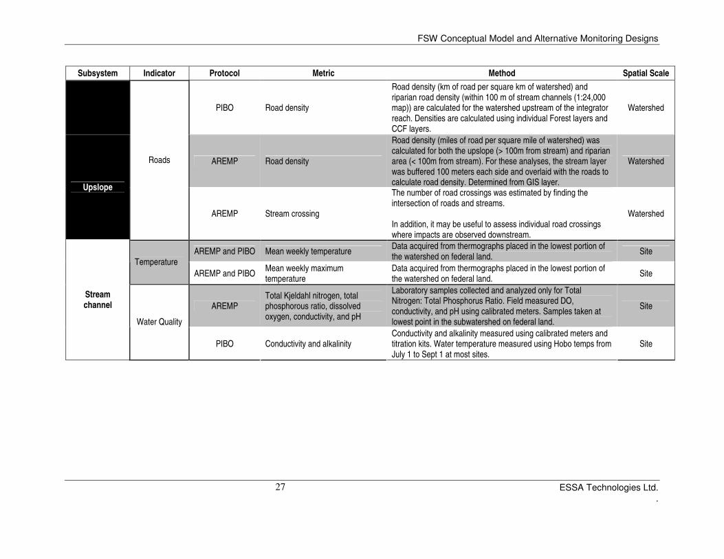
FSW Conceptual Model and Alternative Monitoring Designs
ESSA Technologies Ltd. .
27
Subsystem Indicator Protocol Metric Method Spatial Scale
PIBO Road density
Road density (km of road per square km of watershed) and riparian road density (within 100 m of stream channels (1:24,000 map)) are calculated for the watershed upstream of the integrator reach. Densities are calculated using individual Forest layers and CCF layers.
Watershed
AREMP Road density
Road density (miles of road per square mile of watershed) was calculated for both the upslope (> 100m from stream) and riparian area (< 100m from stream). For these analyses, the stream layer was buffered 100 meters each side and overlaid with the roads to calculate road density. Determined from GIS layer.
Watershed
Upslope
Roads
AREMP Stream crossing
The number of road crossings was estimated by finding the intersection of roads and streams. In addition, it may be useful to assess individual road crossings where impacts are observed downstream.
Watershed
AREMP and PIBO Mean weekly temperature Data acquired from thermographs placed in the lowest portion of the watershed on federal land.
Site Temperature
AREMP and PIBO Mean weekly maximum temperature
Data acquired from thermographs placed in the lowest portion of the watershed on federal land.
Site
AREMP Total Kjeldahl nitrogen, total phosphorous ratio, dissolved oxygen, conductivity, and pH
Laboratory samples collected and analyzed only for Total Nitrogen: Total Phosphorus Ratio. Field measured DO, conductivity, and pH using calibrated meters. Samples taken at lowest point in the subwatershed on federal land.
Site
Stream channel
Water Quality
PIBO Conductivity and alkalinity Conductivity and alkalinity measured using calibrated meters and titration kits. Water temperature measured using Hobo temps from July 1 to Sept 1 at most sites.
Site

FSW Conceptual Model and Alternative Monitoring Designs
ESSA Technologies Ltd. .
28
5.5 Remote sensing protocols
FREP-based inputs to FSW monitoring will likely be integrated with remote sensed information; with
remote sensed information possibly representing the first “tier” of a nested approach to FSW monitoring.
Remote sensed data will be especially important for watersheds whose large size and/or rugged
topography may limit the feasibility of broad-scale, ground-based measurements. Remote sensing is the
observation of habitat features from a distance without actually being in contact with them. It is based on
the principle that objects reflect or emit radiations in different wavelengths and intensities depending on
specific conditions that can be captured by a recording device. An aircraft or satellite may be used for this
purpose equipped with sensors and recording equipment such as cameras, lasers, radar, sonar,
seismographs, gravimeters, etc. Remote sensing can provide an effective alternative to field-based
methods for broadscale monitoring of upslope and/or aquatic habitat within watersheds. Remote sensed
data is being used successfully by many agencies to spatially map and quantify fish habitat and associated
environmental elements, and this data has been incorporated into GIS systems to allow longer term
analyses (e.g., U.S. Forest Service’s Pacific Northwest Aquatic and Riparian Effectiveness Monitoring
Program (AREMP); Reeves et al. 2004). Increasingly remote sensing is being recognized as one of the
most important tools for environmental monitoring, in particular for highly dynamic and vulnerable areas.
There are a number of potential advantages of using remote sensing for habitat evaluation vs. field-based
monitoring. These include: 1) relatively rapid method of acquiring up-to-date information over larger
geographical areas; 2) may be the only practical way to obtain data from inaccessible areas; 3) at some
scales, regional phenomena which are invisible from the ground may be clearly visible; and 4) easy to
manipulate remotely collected data with a computer and combine with other geographic elements in a
GIS. Perceived disadvantages of remote sensing include: 1) cost (although this is dependent on the data
gathering system used and whether it is necessary to incur the cost of deploying remote sensed
technologies or acquiring digital data from pre-existing recording platforms (e.g., continually circling
satellites); 2) acquired data are not direct samples of the habitat, so must be calibrated against reality and
calibration is never exact; and 3) imagery must be corrected geometrically and georeferenced in order to
be useful. This can be easy or complicated.
In British Columbia aerial photography (Terrain Resource Information Management (TRIM) mapping at
the 1:20,000 scale) and low resolution Landsat Thematic Mapper satellite imagery (Baseline Thematic
Mapping (BTM) at the 1:250,000 scale) have been combined and used to categorize watershed habitat
both for the earlier Watersheds BC (BC MELP 2000) and the more recent Ecological Aquatic Units of
British Columbia (EAU BC; Ciruna et al. 2007) mapping exercises. Standard protocols used for these
provincial mapping exercises are available from the website for the province’s Integrated Land
Management Bureau (http://ilmbwww.gov.bc.ca/bmgs/products/). BC MSRM (2001) describes the BTM
procedures, data accuracy and data structure, and defines all land use classes and database schema. BC
MELP (1992) describes the TRIM mapping protocol. These endeavours involved extensive mapping at
the provincial scale, however, and it is uncertain when such mapping would be repeated as an exercise for
the full province. However, Watersheds BC-level mapping and habitat categorizations could be repeated
at various times within different regions of the province, as has been recently done by the MOE for the
Kamloops area (M. Gray, BC Ministry of Agriculture and Lands, pers. comm.) allowing potential
assessment of trends for FSWs in those areas for a wide range of metrics.
It is also feasible to use various remote sensing approaches to identify specific habitat changes over a
range of smaller time scales and spatial extents. Ham (1996) describes the BC Resource Inventory
Committee standards and protocols for aerial photography and videography for stream inventory and
monitoring. Depending upon the scale of study and the detail of information required for channel and

FSW Conceptual Model and Alternative Monitoring Designs
ESSA Technologies Ltd. .
29
habitat assessment, Ham (1996) suggests a variety of surveying techniques can be employed. The choice
of conventional photographic techniques or aerial videography will depend on several factors. The main
things to consider are the size of the study area, the resolution or amount of detail needed, data collection
requirements and total cost. Standard aerial photographs are generally available for most areas of British
Columbia, but recent photographs (i.e., less than 2 years old) may not exist for some areas.
High resolution digital aerial photos combined with thermal infrared imagery can provide even greater
information on habitat features than standard aerial photography and has been used recently by the Alaska
Cooperative Fish and Wildlife Research Unit for monitoring and evaluating dynamic change in large
woody debris in stream channels (Smikrud and Prakash 2006). Airborne Light Detection and Ranging
(LIDAR) technology combined with hyper-spectral imagery has been used to characterize and quantify
aquatic and terrestrial forest habitat and can be used to track broad changes in habitat over variable time
scales (e.g., Hall et al. 2005; Vierling et al. 2008). The Aquatic-Riparian Effectiveness Monitoring
Program (AREMP) developed in the Pacific U.S. (Reeves et al. 2004) employs remote sensed data from
Landsat satellite imagery and techniques outlined in Hemstrom et al. (1998) to evaluate upslope
subsystem indicators (such as vegetation composition, seral stage, and percentage of cover) that reflect
processes influencing the entire stream network and are considered relevant indicators over entire
watersheds. High spatial resolution multi-spectral satellite imagery available from recording platforms
such as Quickbird, IKONOS, SPOT, ASTER, etc. can provide even better information and are also being
increasingly used to classify fish and riparian habitat, and monitor changes of functioning in-river habitat
and riparian structure along stream courses (e.g., Marshall and Storey 2005; Johansen et al. 2007).
BC’s Resource Inventory Committee (BC RIC 1996) describes a standard remote sensed approach for
assessing changing terrain stability and risk of landslides, using the BC Terrain Classification System
(Howes and Kenk 1997) as the basis for air photo interpretation to capture relevant terrain attributes. This
approach could be used to help initial stratification of subbasins within a FSWs into risk categories for
landslides (as was done recently to inform monitoring design for the Bowron River Watershed pilot
study; P. Tschaplinski, BC Ministry of Forests and Range, pers. comm.) or to evaluate change over time.
It may be useful to consider using such remote-sensed evaluations of terrain stability as an initial tier for
assessing any potential deterioration in conditions within individual FSWs, with more intensive field-
based sampling for other metrics then activated in the FSWs of concern. Interpretation of air photos by
experts within the MOFR remains the accepted approach for evaluating terrain stability in provincial
watersheds (P. Jordan, BC Ministry of Forests and Range, pers. comm.) but BC RIC (1996) makes note
of a growing list of remote sensing technologies that could be applied to terrain stability mapping, and
should be investigated over subsequent years. Examples noted that might be applicable for British
Columbia included various types of satellite imagery such as Landsat, SPOT, and European Remote
Sensing Satellites (ERS 1 and 2), as well as airborne radar, multispectral scanners and imaging
spectrometers such as synthetic aperture radar. P. Jordan (BC Ministry of Forests and Range, pers.
comm.) indicated that Quickbird satellites likely provided the best data in this regard, but current high
costs of the digital imagery remains a barrier to its use at this time.
6.0 Approaches/Design options to monitoring watersheds
A successful monitoring program begins with clearly defined objectives; without clear objectives, it is
very difficult to assess the tradeoffs between monitoring approaches. In Appendix D, we propose a
monitoring framework that outlines each of the steps necessary to develop a cost effective and statistically
valid monitoring program. In this section, we introduce the sampling and experimental design concepts
that we feel will be helpful when working through the proposed framework. We focus the discussion on
common concepts and controversies encountered by environmental monitoring programs. Some of the
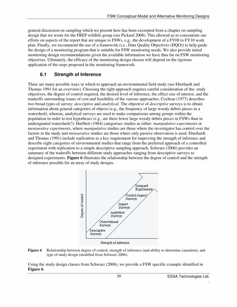
FSW Conceptual Model and Alternative Monitoring Designs
ESSA Technologies Ltd. .
30
general discussion on sampling which we present here has been excerpted from a chapter on sampling
design that we wrote for the FREP wildlife group (see Pickard 2008). This allowed us to concentrate our
efforts on aspects of the report that are unique to FSWs, e.g., the development of a FY08 to FY10 work
plan. Finally, we recommend the use of a framework (i.e., Data Quality Objectives (DQO)) to help guide
the design of a monitoring program that is suitable for FSW monitoring needs. We also provide initial
monitoring design recommendations given the available information we have thus far on FSW monitoring
objectives. Ultimately, the efficacy of the monitoring design chosen will depend on the rigorous
application of the steps proposed in the monitoring framework.
6.1 Strength of Inference
There are many possible ways in which to approach an environmental field study (see Eberhardt and
Thomas 1991 for an overview). Choosing the right approach requires careful consideration of the: study
objectives, the degree of control required, the desired level of inference, the effect size of interest, and the
tradeoffs surrounding issues of cost and feasibility of the various approaches. Cochran (1977) describes
two broad types of survey: descriptive and analytical. The objective of descriptive surveys is to obtain
information about general categories of objects (e.g., the frequency of large woody debris pieces in a
watershed); whereas, analytical surveys are used to make comparisons among groups within the
population in order to test hypotheses (e.g., are there fewer large woody debris pieces in FSWs than in
undesignated watersheds?). Hurlbert (1984) categorises studies as either: manipulative experiments or
mensurative experiments, where manipulative studies are those where the investigator has control over the
factors in the study and mensurative studies are those where only passive observation is used. Eberhardt
and Thomas (1991) include replication as a key requirement for improving the strength of inference and
describe eight categories of environmental studies that range from the preferred approach of a controlled
experiment with replication to a simple descriptive sampling approach. Schwarz (2006) provides an
summary of the tradeoffs between different study approaches ranging from descriptive surveys to
designed experiments. Figure 6 illustrates the relationship between the degree of control and the strength
of inference possible for an array of study designs.
Figure 6 Relationship between degree of control, strength of inference (and ability to determine causation), and
type of study design (modified from Schwarz 2006).
Using the study design classes from Schwarz (2006), we provide a FSW specific example identified in
Figure 6.

FSW Conceptual Model and Alternative Monitoring Designs
ESSA Technologies Ltd. .
31
Descriptive study: A FSW is selected and an indicator, e.g., road density, is measured. The information
collected is only relevant to the watershed sampled.
Observational study: A non-designated watershed and a FSW are selected; road density is measured in
both. Comparisons between the two watersheds can be made, but the results are only applicable to the two
watersheds sampled. Using this approach, it is not possible to conclude whether any observed differences
are representative of the differences between the two categories of watersheds. Descriptive and
observational studies involve non-randomly selected sampling units; as a result the information obtained
is limited to the sites actually observed.
Analytical survey: A random sample of watersheds from each category is selected and road density is
measured in each watershed. An estimate of the mean road density with known precision can be obtained
for each category. The estimates from the two categories can be compared; however, it is possible that
another unknown factor (besides FSW designation) is actually responsible for the difference.
Impact and control-impact surveys: The goal of this approach is to assess the impact of some change,
in this case the designation of a watershed as ‘Fisheries Sensitive’. A variety of impact designs with
increasing levels of effort and increasing degrees of inference exist. Mellina and Hinch (1995) provide a
summary of different impact designs and describe how each might be used to assess watershed
restoration. Schwarz (2006) and Underwood (1994) provide a good description along with examples for a
range of impact studies, as well as evaluating their respective strengths and weaknesses. The simplest
impact studies look at a single location before and after some event. Obtaining multiple observations
before and after an event improves the ability to determine if an observed change is ‘real’ by taking into
account the natural year to year variability. Since obtaining ‘before’ samples is often difficult, it may be
possible to get variance estimates by randomly sampling from similar but undisturbed habitats
(Underwood 1994). This approach can be considerably improved by adding a control site, where the
control watershed (an undesignated watershed) is similar to the treatment watershed (i.e., FSW) with
respect to general watershed characteristics (e.g., region, annual precipitation, size, etc.). This approach is
termed a ‘Before After Control Impact’ (BACI) design. BACI designs are intended to address the
question of whether a particular action has resulted in a change at the treatment/impact site relative to the
control site, while simultaneously adjusting for extraneous co-variables that might be similarly affecting
both impact and control areas. In most cases, the use of controls greatly increases the power of detecting
treatment/impact effects; however, poorly chosen control sites can decrease the power of detecting an
effect (Korman and Higgins 1997; Roni et al. 2003). For example, a lack of randomization in assigning
impact sites prevents us from inferring whether the impact will occur elsewhere. Alternatively, if there is
only a single impact/control pair, how do we know that the results are not just a consequence of the
choice of sites?
Keough and Mapstone (1995) further extend the BACI design to contain multiple controls and if possible
multiple impact sites; referred to as MBACI (Downes et al. 2002). In a MBACI design multiple treatment
and control locations are chosen randomly from a group of potential locations, thereby providing the
means to extrapolate to a larger area. If it is not possible to randomly assign treatments and controls, but
the same pattern is observed in multiple pairs, it is reasonable to assign a causal relationship (Schwarz
2006).
Designed experiments: In a designed experiment, the investigator has control over the treatment and can
randomly assign experimental units to treatments. The degree of control the investigator has on a study
affects the ability to show causation. The ability to make inference to other sampling units depends on
random selection of samples or assignment of treatments.

FSW Conceptual Model and Alternative Monitoring Designs
ESSA Technologies Ltd. .
32
6.2 Review of Sampling Approaches
6.2.1 Basic probabilistic sampling designs1
The target population can be defined in several ways: 1) the complete collection of individuals we wish
to study (Lohr 1999); 2) the population about which information is wanted (Cochran 1977); and 3) the
complete set of units about which we want to make inferences (Elzinga et al 2001). Regardless of
definition, in order to make inferences about the entire target population, all individuals within the target
population must have some chance of being selected in the sample. The sampling population or sampling
frame is the collection of all possible sampling units that might have been chosen in a sample, or can
alternatively be described as the population from which the sample was taken (Lohr 1999). Probabilistic
sampling refers to designs in which each sampling unit within the sampling frame has a known and non-
zero probability of being selected. There are two probabilistic sampling designs that are most commonly
used and form the basic building blocks of most sampling designs: simple random sampling (SRS), and
systematic random sampling (SysRS). SRS refers to the situation where a random sample of all sampling
units within the sampling frame is selected (e.g., drawing numbers from a hat). SysRS refers to the
situation where sampling units are selected at regular intervals using a randomly selected starting point,
e.g., reading every tenth name from the phone book or taking a sample every ten metres.
6.2.2 Variations on the basic probabilistic designs2
There are multiple variations of these basic designs that have been developed to address particular
situations including: cluster sampling, adaptive sampling, and distance sampling.
• In a cluster sample, an initial random sample of sites is chosen and then a census is completed
within that site (e.g., a random sample of pools with a census of body weight/length of all fish
found in the pool).
• Adaptive sampling begins like any other sampling design with a random selection of sampling
units, but additional sampling units may be added based on the observed values in the initial
sample (Thompson 1990).
• Generalized random-tessellation stratified (GRTS) designs are a recent approach that draws on
the strengths of each of the basic designs. GRTS designs are spatially-balanced probabilistic
surveys developed by the US Environmental Protection Agency (EPA) under their Environmental
Monitoring and Assessment Program (Stevens & Olsen 2004).
Stratification is a tool which can be applied to any sampling design. In a stratified random design the
sampling frame is divided into non-overlapping groups (strata) based on some characteristic such as sex
or habitat type. A random sample is then chosen from each of the strata.
Any combination of these designs can be used in a multi-stage sampling design. For example, a simple
random sample of streams could be chosen from each stratum within the target population. A systematic
random sample of reaches within each stream could then be selected, followed by a census or sample of a
particular metric (e.g., large woody debris) within each reach. Calculating an estimate of the mean from a
multi-stage sample is fairly intuitive, but the variance calculations are more complicated. A typical
mistake made is a form of pseudo-replication discussed by Hurlbert (1984), where all observations are
treated as though they were drawn at random from the target population. In reality the secondary
sampling units (reaches in this case) are a sample from the stream, not the population. Increasing the
1 Modified from Pickard (2008). 2 Modified from Pickard (2008).

FSW Conceptual Model and Alternative Monitoring Designs
ESSA Technologies Ltd. .
33
number of reaches within streams helps improve the precision of the estimate for the single stream, but
will not necessarily improve the estimate of the strata unless additional streams are sampled.
6.2.3 Choosing an appropriate probabilistic sampling design
Sampling research and development is typically focused on finding more efficient designs, where the goal
is to obtain precise estimates without spending too much money. A SRS assumes no knowledge of the
system and allocates effort at random to the entire sampling frame. Other sampling designs and tools
incorporate information like the cost of moving between sites and the recognition that not as many
replicates are needed in relatively homogeneous strata. A SRS can always be used, but may not always be
the most efficient choice. For example, for a fixed cost you can take more samples in a cluster survey, so
the final precision can be better than from a SRS of the same cost (Cochran 1977). Stratification on the
other hand, may result in a more efficient design when there is less variability within strata than between
strata (Cochran 1977; Lohr 1999). Stratification may also be useful if estimates for individual strata are
desired as well as for the entire population. If the target population changes proportional to position (e.g.,
samples taken upstream vs. downstream) a SysRS may be an appropriate way to ensure spatial coverage.
If the population of interest is randomly distributed then the SysRS approximates the SRS (Lohr 1999). If
the target population displays regular or cyclical characteristics then a SysRS is a poor choice. GRTS
overcomes some of the shortcomings of both SRS (which tends to “clump” sampling sites) and SysRS by
generating an ordered, spatially balanced and unbiased set of sites that represent the population from
which the sample sites will be drawn.
6.2.4 Comparison of SRS, SysRS, and GRTS
The FSW monitoring program has a broad geographic scope (province of BC); consequently, the cost of
moving between sites will likely be substantial. In addition, the diversity of ecosystems present in BC (14
bio-geoclimatic zones) makes it important to ensure proper spatial coverage of sample sites. The GRTS
approach provides a nice alternative that can deal with some of the complications that arise in practice
when using either SRS or SysRS. We provide a brief comparison of these three approaches (Tables 4 to
11).
Table 4 Comparison of SRS, SysRS, and GRTS estimates if precision
Approach Description
SRS Simple to compute
SysRS
A proper estimate of precision is very difficult to compute for a (single) systematic sample unless you are willing to make strong assumptions about self-randomization (in which case a systematic sample is equivalent to an SRS) or have knowledge about any "trend" in the population that the systematic sample can measure. To get around these issues, replicated systematic samples are often done. For example, rather than taking a single systematic sample of size 100, you may take 4 independent systematic samples of 25. Compute an estimate from each systematic sample of size 25 and then the variance in the 4 estimates can be used to get an overall SE
GRTS Slightly more complicated than SRS and SysRS, but Stevens and Olsen (2004) give details on computations of simpler forms and the R library (spsurvey) documents the analytical tools.
Dealing with "refusals" or “non-response”: In many cases, after the sample points (locations) have
been selected it is not possible to use them (e.g., because landowners will not give permission, they are
inaccessible, or the location is not safe). Each approach deals with this scenario differently and some are
more robust to the problem than others (Table 5).
Table 5 Comparison of SRS, SysRS, and GRTS under “refusals” or “non-response” scenario.
Approach Description
SRS Simply draw a new point at random. There is no impact on variance computations. SysRS Non-response is a problem for this design. You cannot simply choose another point and all the formulae

FSW Conceptual Model and Alternative Monitoring Designs
ESSA Technologies Ltd. .
34
for estimates are affected because of the missing data. You could over sample, but now the gaps will be unequally spaced in the data.
GRTS Robust to this problem because it allows over sampling (Theobold et al. 2007). Simply choose the next point (after reverse hierarchal ordering). This is equivalent to SRS simply choosing another point.
Accommodating different sampling intensities: In some cases, two different "surveys" are to be
conducted simultaneously with different sampling intensities. For example, you may wish to sample 25
points for survey A and 100 points for survey B. Each sampling method requires a slightly different
procedure that is outlined in Table 6.
Table 6 Procedure for accommodating different sampling regimes when using SRS, SysRS, and GRTS.
Approach Description
SRS Draw 100 points for survey B, and then randomly select 25 from those 100 for survey A. This way 25 points get both A and B; and the remaining 75 points get B only. Both are SRS so it is easy to compute estimates and variance.
SysRS Draw SysRS of size 100, and then do a second SysRS of size 25 from those 100 points chosen. Both are systematic samples with same problems in dealing with missing data and variance computation.
GRTS Draw first 100 in reverse hierarchical ordering for B. Use first 25 for A. Both samples are GRTS, so no problems in computing estimates and variance.
Spatial coverage: If there is correlation among units (i.e., units close together will tend to be more
similar than units further apart), then a sampling design with good spatial coverage is a good thing. When
spatial correlation exists there is no need to sample two points very close together as they will tend to
have the same response and would lead to "wasting" of samples. Generally, when a correlation between
units is present, designs that are more spatially spread out will tend to have better precision (i.e., lower
SE) than SRS because there is no "wasting" of samples at points that are close together. Table 7 outlines
the ability of each approach to take into account spatial coverage.
Table 7 Comparison of spatial coverage of SRS, SysRS, and GRTS approaches.
Approach Description
SRS Poor spatial coverage. Any single realization of a SRS often results in areas with clusters of samples and areas with no samples (Theobold et al. 2007).
SysRS High spatial coverage. The problem with SysRS designs is that in the presence of "correlation" among units, it is not clear how to compute the variance for a systematic design.
GRTS Intermediate between both. The way the GRTS is taken tends to spread samples out more than an SRS but not as regularly as a SysRS.
Variable selection probabilities: For example, if sampling units are of different sizes, e.g., watersheds, it
may be preferable to have the probability of selection proportional to the size of the watershed, under the
assumption that larger watersheds contribute more to the overall quality of a regional habitat than very
small watersheds. The ease of varying selection probability using each method is discussed in Table 8.
Table 8 Comparison of SRS, SysRS, and GRTS approaches when using variable selection probabilities.
Approach Description
SRS Need to switch selection probabilities so they are proportional to size, but computations are straight forward.
SysRS Need to switch to a systematic sample on the size variable, but now estimates and variance issues are much more complicated.
GRTS Need to switch selection probabilities so they are proportional to size, but computations are straight forward.
Inverse sampling: When using inverse sampling, units are selected one at a time until some preset
criteria is met, i.e., at least 10 sites with a special attribute that cannot be identified in advance. If you

FSW Conceptual Model and Alternative Monitoring Designs
ESSA Technologies Ltd. .
35
could identify the attribute in advance, then it is more efficient to use the attribute as a stratification
variable. Table 9 outlines the relative ease or difficulty of using inverse sampling with each approach.
Table 9 Comparison of SRS, SysRS, and GRTS approaches and inverse sampling
Approach Description
SRS Not a problem, just draw one unit at a time. SysRS Not clear how to do this.
GRTS Not a problem, just select units one at a time in reverse hierarchical ordering. Some care needs to be taken in computing variances as "n" is now random, but this is usually ignored and the actual sample size "n" is treated as specified in advance.
Stratification: As described in Section 6.2.2, stratification can be a useful tool for improving the
efficiency of a design (see Table 10 for a comparison of stratification using alternative methods).
Table 10 Comparison of SRS, SysRS, and GRTS approaches and stratification.
Approach Description
SRS No problem SysRS No problem GRTS No problem; can be applied to the GRTS in much the same way as any other design.
Dealing with continuous sampling units: As described in Section 6.2.1, the target population and
sampling unit need to be defined. In some cases the target population does not have any obvious splits to
separate into sampling units. For example, rivers are "continuous", i.e., they do not have fixed sampling
stations, so how should a river be split into sampling units? Table 11 lists how each method would deal
with continuous sampling units
Table 11 Comparison of SRS, SysRS, and GRTS approaches with continuous sampling units.
Approach Description
SRS Discretize streams into individual points, or arrange on a line (like GRTS) and take SRS of points on the line.
SysRS Same as above. GRTS Same as above.
Creating and implementing a GRTS design can be difficult, as the estimate and variance calculations are
complicated and hand computations are not really feasible. It is also difficult to generate a spatially
explicit sampling frame for a large geographic scale; however, GIS technology has made this possible and
relatively straightforward. The actual generation of sampling frames depends on the study objectives,
target populations, and the extent to which the digital coverage reflects the target population (as it would
with any design). The selection of a GRTS sample and the computations have been automated to a great
extent. Software packages required to create GRTS designs include psurvey.design (free for download
from the U.S. Environmental Protection Agency (EPA) Aquatic Resources Monitoring website
(http://www.epa.gov/nheerl/arm/designing/design_intro.htm), R statistical package and ArcGIS)
6.2.5 Judgement or non-probabilistic designs3
Judgement samples are selected subjectively. Sites may be chosen according to some prior belief about
where individuals should be found, they may be chosen arbitrarily to be representative of the target
population, or they may be chosen just for convenience. So called ‘representative reaches’ in stream
surveys are an example of a judgment sample; however, without a census of the target population (e.g.,
the entire stream), it is impossible to be sure that you have chosen a representative sample reach.
3 Modified from Pickard (2008).

FSW Conceptual Model and Alternative Monitoring Designs
ESSA Technologies Ltd. .
36
McDonald (2004) describes many examples where allocating some effort outside supposed core areas
provided considerable improvement in the understanding of distribution and estimates of abundance for
rare and elusive populations. For example, if core habitat had relatively consistent densities, while
marginal habitat density fluctuated with the size of the population, then ignoring the marginal habitat
would mask the true health of the population. Sometimes sites that are thought to be particularly sensitive
‘sentinel sites’ are selected for monitoring, but this too is a controversial issue (Edwards 1998). Making
inference from judgment samples has lead, for example, to some famous miscalculations in predicting
election results (Edwards 1998).
6.3 Timing and frequency of sampling4
The question of whether samples should be collected daily, monthly, annually, every 10 years, etc. is an
important one to address. The appropriate sampling frequency will differ by study objective and the
subject of interest. Is the study interested in a one-time estimate of status, or is the objective to monitor
the species, community, or habitat over time? In ecological studies the temporal scale of interest is often
annual (i.e., annual estimates of abundance, health, survival etc.). These estimates can be combined into
multi-year studies that allow for estimates of trends over time and comparisons between years. There are
a number of interesting and challenging statistical design questions that arise depending on the temporal
scale of interest.
Within a year:
When and how often should sampling be done within a year in order to obtain annual estimates? The
answer will ultimately depend on the life history of the species of interest, the ecology of the system, and
the target population. In general the optimal time to sample an organism or object is when the probability
of detection is the greatest, either due to behaviour, colour (i.e., mating colouration or vegetation
colouration), time of day, or season. When sampling a characteristic that varies seasonally, and/or daily,
e.g., temperature, stream flow, or vegetation cover, it is important to be consistent with the timing of
sampling and reporting of the metric. It might be best to choose the time of day or year which is
considered to be of most importance to the organism or ecology of the system, e.g., maximum summer
water temperature or vegetation cover during the most predator susceptible months. Alternatively, a
summary statistic, such as monthly or annual mean precipitation, could be used.
Long-term monitoring programs:
Sampling designs spanning multiple years are important when trying to consider changes to individuals or
populations over time. There are many conflicting opinions about how sampling designs over time should
be implemented. A major discussion point is whether permanent (long-term) or temporary sites should be
selected. The typical response is to use permanent sites for trend detection and temporary sites for status
assessment; however, in reality it is rarely that simple. There are advantages and disadvantages to each
approach and researchers differ in their opinions of which approach to take. A brief summary of the
advantages and disadvantages of each approach are described in Pickard (2008).
McDonald (2003) found that the term ‘trend’ is used in different ways by different researchers; perhaps
this is the source of some of the controversy around ‘permanent vs. temporary’ sites. For example, what
scale is the change of interest: reach, stream, watershed, or province? McDonald (2003) provides several
useful definitions that may be helpful in clarifying the study objective and hence determining the best
design:
4 Modified from Pickard (2008).

FSW Conceptual Model and Alternative Monitoring Designs
ESSA Technologies Ltd. .
37
Net change: measurement of total change in a parameter arising from all sources
• change in mean or total response
• individual change can happen without causing net change, e.g., fish move from one stream
segment to another, where individual stream segments could experience a trend while the
overall population of the watershed does not.
Individual change: change experienced by an individual or particular member of the population, this
can be further divided into three categories:
• gross change: change in response of a particular population unit (e.g., change in pH of a
particular lake)
• average gross change: if all rivers in a collection of rivers have higher levels of suspended
sediment (i.e., the same change occurs to many individual units)
• instability: variance of responses from individual population units
An alternative which has recently been popularized, but which has been discussed for some time (see
Jessen 1942; Cochran 1977), is to use a design with some combination of repeated visits and new sites.
This type of approach has been referred to by a number of names, e.g., revisit, repeated, rotating, split-
panel, and replacement. McDonald (2003) provides an excellent review of these designs and develops
consistent terminology. These designs provide a compromise between temporary and permanent sites that
allow the estimation of both status and trends. McDonald (2003) found that “consensus opinion among
the reviewed articles appeared to be that some sort of split-panel design had the best chance of satisfying
the sometimes competing objectives inherent in many environmental monitoring projects”. A few
definitions from McDonald (2003) are helpful:
Panel: A group of population units that are always all sampled during the same sampling occasion or
time period. Note that a population unit may be a member of more than one panel under this
definition.
Revisit design: The rotation of sampling effort among survey panels. The pattern of visits to the
panel. The plan by which population units are visited and sampled through time.
Membership design: The method used to populate the survey panels. The way in which units of the
population become members of a panel.
Implementing and analyzing these designs can be difficult. The analysis is complicated and a qualified
statistician should be consulted. Any design which extends over many years will require consistent
funding and good documentation to allow for transition between people, priorities and political shifts.
While these designs in general are recommended, the specific frequency of return visits and the sample
sizes required depends on the specific study and the ecology of the subject. Generally, it is recommended
that if trend is the primary objective >50% of sampling effort should be allocated to the revisited sites; if
both status and trends are important then the sampling effort should be allocated equally to the revisited
and new panels (McDonald 2003). Urquhart and Kincaid (1999) found that for trend detection, some
panel designs in which not all sites are visited every year can be nearly as powerful as designs in which
every site is revisited every year. More research is needed to address the optimal allocation of sampling
effort among panels (McDonald 2003). Dr. Stevens of the Oregon State University Department of
Statistics is currently focusing on the question of trend detection taking advantage of panel designs
(David P. Larsen, US EPA, pers. comm.).

FSW Conceptual Model and Alternative Monitoring Designs
ESSA Technologies Ltd. .
38
6.4 Recommendations
We provide a set of preliminary recommendations for the creation of a FSW monitoring program.
Detailed recommendations cannot yet be made because they require greater refinement of and clarity
around the study questions (Section 4.0). However, if one management question of the monitoring
program is to determine whether or not designating a watershed as a FSW is an effective management
action, then the study design should provide evidence of causation as well as a strong level of inference.
The monitoring program therefore needs to be as close to a designed experiment as possible. In addition,
the observed watersheds should be selected randomly so that inferences to the population of all
watersheds can be made.
The FSW monitoring program could be a true designed experiment if investigators are willing to leave
some otherwise FSW eligible watersheds as unprotected controls, in addition to assigning FSW
designation and control status at random. However, a designed experiment of this kind may not be
feasible given the nature of the process required to designate FSW and some form of replicated BACI
design is probably adequate for assessing FSW benefits. Increasing the number of years of data collection
prior and post FSW designation would increase the power to detect a difference between FSWs and non-
FSWs. In addition, increasing the number of control/impact watersheds would increase the confidence
that any change observed is a result of the FSW management action. The exact number of years and sites
necessary is something that needs to determined and will depend on completion of earlier work plan
steps. Keely and Walters (1994) recommend a sample of 8 to 16 streams, for 4 to 8 years to assess the
success of watershed restoration actions. The sample size and duration necessary will depend to some
extent on the magnitude of the treatment. If the treatment is passive, as appears to be the case for FSWs, it
will likely take much longer to see a response/difference than that predicted for an active watershed
restoration program.
To move forward on developing monitoring designs, FSW management actions must be clearly defined.
It is not yet apparent to what extent forestry, mining, and/or grazing activities within FSW designated
watersheds will differ from those without any designation. Clarification on this issue is important because
it will be extremely difficult to detect an effect as a consequence of FSW designation in a reasonable
timeframe unless there is sufficient contrast between the management of the FSW and control watersheds.
Access to, and examination of, the content of licensee’s Forest Stewardship Plans (FSPs; including
supporting documents) will be a critical step in deriving this information5. Even more contrast is required
if the intent of monitoring is to try and distinguish between different types of actions within watersheds
(e.g., forestry vs. mining). It may therefore be preferable to complete a designed experiment on a random
subset of watersheds, where more extreme management actions (e.g., increased riparian buffer, halt in
mining activity, etc.) are implemented that we can learn what types of management actions would be
effective in protecting watershed processes within FSWs.
It is important to build upon the FREP program in order to allow comparisons with FREP results and
where possible to provide more efficient data collection. FREP protocols should be used where
information needs overlap (e.g., approximately 44 metrics used by FREP could be used for FSW
monitoring; see Table 2). Using the same protocols has several advantages some of which include: the
data collected is comparable and can be used for either program; and field crews only need to be trained
in one protocol therefore helping to minimise operator error. There are however several issues that need
to be resolved when trying to incorporate FREP concepts into an FSW monitoring program. The largest
5 Individual FSPs use different strategies to meet the desired condition set out in FSW orders. Consequently, it may
not be possible to determine how management actions in FSW differ from those in non-FSW because of insufficient
contrast.
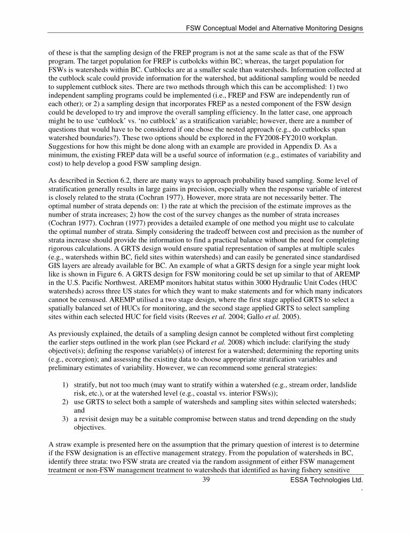
FSW Conceptual Model and Alternative Monitoring Designs
ESSA Technologies Ltd. .
39
of these is that the sampling design of the FREP program is not at the same scale as that of the FSW
program. The target population for FREP is cutbolcks within BC; whereas, the target population for
FSWs is watersheds within BC. Cutblocks are at a smaller scale than watersheds. Information collected at
the cutblock scale could provide information for the watershed, but additional sampling would be needed
to supplement cutblock sites. There are two methods through which this can be accomplished: 1) two
independent sampling programs could be implemented (i.e., FREP and FSW are independently run of
each other); or 2) a sampling design that incorporates FREP as a nested component of the FSW design
could be developed to try and improve the overall sampling efficiency. In the latter case, one approach
might be to use ‘cutblock’ vs. ‘no cutblock’ as a stratification variable; however, there are a number of
questions that would have to be considered if one chose the nested approach (e.g., do cutblocks span
watershed boundaries?). These two options should be explored in the FY2008-FY2010 workplan.
Suggestions for how this might be done along with an example are provided in Appendix D. As a
minimum, the existing FREP data will be a useful source of information (e.g., estimates of variability and
cost) to help develop a good FSW sampling design.
As described in Section 6.2, there are many ways to approach probability based sampling. Some level of
stratification generally results in large gains in precision, especially when the response variable of interest
is closely related to the strata (Cochran 1977). However, more strata are not necessarily better. The
optimal number of strata depends on: 1) the rate at which the precision of the estimate improves as the
number of strata increases; 2) how the cost of the survey changes as the number of strata increases
(Cochran 1977). Cochran (1977) provides a detailed example of one method you might use to calculate
the optimal number of strata. Simply considering the tradeoff between cost and precision as the number of
strata increase should provide the information to find a practical balance without the need for completing
rigorous calculations. A GRTS design would ensure spatial representation of samples at multiple scales
(e.g., watersheds within BC, field sites within watersheds) and can easily be generated since standardised
GIS layers are already available for BC. An example of what a GRTS design for a single year might look
like is shown in Figure 6. A GRTS design for FSW monitoring could be set up similar to that of AREMP
in the U.S. Pacific Northwest. AREMP monitors habitat status within 3000 Hydraulic Unit Codes (HUC
watersheds) across three US states for which they want to make statements and for which many indicators
cannot be censused. AREMP utilised a two stage design, where the first stage applied GRTS to select a
spatially balanced set of HUCs for monitoring, and the second stage applied GRTS to select sampling
sites within each selected HUC for field visits (Reeves et al. 2004; Gallo et al. 2005).
As previously explained, the details of a sampling design cannot be completed without first completing
the earlier steps outlined in the work plan (see Pickard et al. 2008) which include: clarifying the study
objective(s); defining the response variable(s) of interest for a watershed; determining the reporting units
(e.g., ecoregion); and assessing the existing data to choose appropriate stratification variables and
preliminary estimates of variability. However, we can recommend some general strategies:
1) stratify, but not too much (may want to stratify within a watershed (e.g., stream order, landslide
risk, etc.), or at the watershed level (e.g., coastal vs. interior FSWs));
2) use GRTS to select both a sample of watersheds and sampling sites within selected watersheds;
and
3) a revisit design may be a suitable compromise between status and trend depending on the study
objectives.
A straw example is presented here on the assumption that the primary question of interest is to determine
if the FSW designation is an effective management strategy. From the population of watersheds in BC,
identify three strata: two FSW strata are created via the random assignment of either FSW management
treatment or non-FSW management treatment to watersheds that identified as having fishery sensitive

FSW Conceptual Model and Alternative Monitoring Designs
ESSA Technologies Ltd. .
40
value; and the third stratum is the remainder of watersheds which were not designated as either FSW or
non-FSW and which do not have fishery sensitive value. A two stage sampling design is implemented.
First, a GRTS sample of watershed from within each strata is selected and second, a GRTS sample of
stream reaches is selected from within the watershed (see Figure 7)
FSW Conceptual Model and Alternative Monitoring Designs
ESSA Technologies Ltd. .
41
Figure 7 Example of an experimental design using GRTS selected sampling points outside and within a subset of 31 currently designated Fisheries Sensitive
Watersheds (FSWs). Shown are GRTS selected sample points: 1) outside the boundaries of the FSWs (n=30, red points); 2) distributed within
treatment FSWs (n=18; shaded yellow, 100 brown points); and 3) within non-treated FSWs (n = 15; shaded blue, 30 green points), using the
province’s 1:50,000 stream reach hydrology network as the underlying sample frame.
FSW Conceptual Model and Alternative Monitoring Designs
ESSA Technologies Ltd. .
42
7.0 Works cited
Angermeier, P.L., A.P. Wheeler, A.E. Rosenberger. 2004. A conceptual framework for assessing impacts
of roads on aquatic biota. Fisheries 29(12): 19-29.
Alberti, M., D. Booth, K. Hill, B. Coburn, C. Avolio, S. Coed, and D. Spirandelli. 2007. The impact of
urban patterns on aquatic ecosystems: an empirical analysis in Puget lowland sub-basins.
Landscape and Urban Planning 80: 345-361.
Barbour, M.T., J. Gerritsen, B.D. Snyder, and J.B. Stribling. 1999. Rapid Bioassessment Protocols for
Use in Streams and Wadeable Rivers: Periphyton, Benthic Macroinvertebrates and Fish, Second
Edition. EPA 841-B-99-002. U.S. Environmental Protection Agency; Office of Water;
Washington, D.C.
B.C. Ministry of Environment Lands and Parks (BC MELP). 2000. Watersheds BC User’s Guide.
Geographic Data BC.
B.C. Ministry of Environment (BC MOE). 1992. Digital baseline mapping at 1:20,000. Release 2.0.
British Columbia Specifications and Guidelines for Geomatics. Content Series Volume 3.
Geographic Data BC. Available at: http://ilmbwww.gov.bc.ca/bmgs/pba/trim/specs/specs20.pdf
B.C. Ministry of Environment (BC MOE). 2007. Watershed Evaluation Tool (v3) Method Description.
Prepared by Ecosystem Planning Section, B.C. Ministry of Environment, Victoria, BC.
B.C. Ministry of Forests and Range (BC MFR). 2007. What is FREP?. Available at:
http://www.for.gov.bc.ca/hfp/frep/about/index.htm. Accessed: March 18th, 2008.
B.C. Ministry of Sustainable Resource Management (BC MSRM). 2001. baseline thematic mapping
present land use at 1:250,000. Release 2.1. British Columbia Specifications and Guidelines for
Geomatics. Content Series Volume 6, Part 1. Geographic Data BC. Available at:
http://ilmbwww.gov.bc.ca/cis/initiatives/ias/btm/btm2specaug1.pdf
B.C. Resource Inventory Committee (BC RIC). 1996. Terrain stability mapping in BC: a review and
suggested methods for landslide hazard and risk mapping – final draft. The Province of BC.
Available at: http://ilmbwww.gov.bc.ca/risc/pubs/earthsci/terrain2/index.htm
Bilby, R. and P. A. Bisson, 1998. function and distribution of large woody debris. In: River Ecology and
Management: Lessons from the Pacific Coastal Ecoregion, R. Naiman & R. Bilby, (Editors).
Springer-Verlag, New York, pp. 324-346.
Bjornn, T.C., and D.W. Reiser. 1991. Habitat requirements of salmonids in streams. American Fisheries
Society Special Publication 19: 83-138.
Borstad, G., L. Brown, P. Willis, J. Irvine, and S. Akenhead. 2007. Satellite Based Indicators of
watershed changes: some early results. Conference preseantation.

FSW Conceptual Model and Alternative Monitoring Designs
ESSA Technologies Ltd. .
43
Brannon, E.L., M.S. Powell, T.P. Quinn, and A. Talbot. Population structure of Columbia River Basin
chinook salmon and steelhead trout. Rev. Fish. Sci., 12: 99–232 (2004).
Brown, G.W., and J.T. Krygier. 1970. Effects of clear-cutting on stream temperature. Water Resources
Research 6: 1133-1139.
Bury, R.B. 2004. Low thermal tolerances of stream amphibians in the Pacific Northwest: Implications for
riparian and forest management. Applied Herpetology 5: 63-74
Carson, B., D. Maloney, S Chatwin, M. Carver and P. Beaudry. 2008. Protocol for Evaluating the
Potential Impact of Foresty and Range Use on Water Quality (Water Quality Routine
Effectiveness Evaluation). Forest and Range Evaluation Program, B.C. Min. For. Range and B.C.
Min. Env., Victoria, BC.
Chamberlin, T.W., R.D. Harr, and F.H. Everest. 1991. Timber harvesting, silviculture, and watershed
processes. American Fisheries Society Special Publication 19: 83-138.
Ciruna, K.A., B. Butterfield, J.D. MacPhail, and BC Ministry of Environment. 2007. EAUBC: Ecological
Aquatic Units of British Columbia. Prepared by the Nature Conservancy of Canada. Toronto,
Ontario. 200 pp.
Cochran, W.G. 1977. Sampling Techniques. John Wiley & Sons, Inc., New York, NY.
Collins, J.N., E.D. Stein, M.Sutula, R. Clark, A.E. Fetscher, L. Grenier, C.Grosso, and A. Wiskind. 2007.
California rapid assessment method (CRAM) for wetlands. Version 5.0.1. 151 pp.
Collaborative Systmwide Monitoring and Evaluation Program (CSMEP). 2005. CSMEP Habitat
Subgroup Steps 6 and 7 of the DQO Process: Lemhi Habitat Compensation Program Example.
Columbia Basin Fish and Wildlife Authority, Portland, OR.
Available at:
http://www.cbfwa.org/Committees/CSMEP/documents/ReferenceDocuments/HabitatDQO-
Steps6-7Dec21_draft_groupFinal.doc
Downes, B.J., L.A. Barmuta, P.G. Fairweather, D.P. Faith, M.J. Keough, P.S. Lake, B.D. Mapstone and
G.P. Quinn. 2002. Monitoring ecological impacts: concepts and practice in flowing waters.
Cambridge University Press, Cambridge, UK.
Eberhardt, L.L., and J.M. Thomas. 1991. Designing Environmental Field Studies. Ecological Monographs
61:53-73.
Edwards, D. 1998. Issues and themes for natural resources trend and change detection. Ecological
Applications 8(2): 323–325
Elzinga, C.L., Daniel W. Salzer, John W. Willoughby, and James P. Gibbs. 2001. Monitoring plant and
animal populations. Blackwell Science, Inc., Malden, Massachusetts.
Engle, S.R., and J.R. Voshell. 2002. Volunteer biological monitoring: can it accurately assess the
ecological condition of streams? American Entomologist: 48(3): 164-177.

FSW Conceptual Model and Alternative Monitoring Designs
ESSA Technologies Ltd. .
44
Fennessy M.S., A.D. Jacobs, and M.E. Kentula. 2007. An evaluation of rapid methods for assessing the
ecological condition of wetlands. Wetlands 27(3): 543-560.
Fennessy, M.S., A.D. Jacobs, and M.E. Kentula. 2004. Review of Rapid Methods for Assessing Wetland
Condition. EPA/620/R-04/009. U.S. Environmental Protection Agency, Washington, D.C.
Fore, L.S. 2003. Developing Biological Indicators: lessons learned from mid-atlantic streams. Prepared
for: U.S. Environmental Protection Agency, Environmental Science Center, Ft. Meade, MD.
EPA/903/R-03/003. Available at: www.epa.gov/maia/html/llstream.htm
Fausch, K.D., and Northcote, T.G. 1992. Large woody debris and salmonid habitat in a small coastal
British Columbia stream. Can. J. Fish. Aquat. Sci. 49: 682–693.
Furniss, M.J., T.D. Roelofs, and C.S. Yee. 1991. Habitat requirements of salmonids in streams. American
Fisheries Society Special Publication 19: 297-323.
Gallo, K, S.H. Lanigan, P. Eldred, S.N. Gordon, C. Moyer. 2005. Northwest Forest Plan—the first 10
years (1994-2003): preliminary assessment of the condition of watersheds. Gen. Tech. Rep.
PNW-GTR-647. Portland, OR: U.S. Department of Agriculture, Forest Service, Pacific
Northwest Research Station. 133p.
Gende, S.M., R.T. Edwards, M.F. Willson, and M.S. Wipfli. 2002. Pacific Salmon in Aquatic and
Terrestrial Ecosystems. BioScience 52(10): 917-928.
Grant, J.W.A., Englert, J., and Bietz, B.F. 1986. Application of a method for assessing the impact of
watershed practices: effects of logging on salmonid standing crops. North Am. J. Fish. Manage.
6: 24–31.
Griffith, J., E. Martinko, J. Whistler, and K. Price. 2002. “Interrelationships among landscapes, NDVI,
and stream condition in the U.S. Central Plains.” Ecological Applications 12(6): 1702-1718.
Growns J.E., B.C. Chessman, J.E. Jackson, et al. 1997. Rapid assessment of Australian rivers using
macroinvertebrates: cost and efficiency of 6 methods of sample processing. Journal of the North
American Benthological Society 16(3): 682 – 693.
Gucinski, H., M.J. Furniss, R.R. Ziemer, and M.H. Brookes. 2001. Forest roads: A synthesis of scientific
information. PNW-GTR-509, Portland, Or.
Hall, R.K., R. Watkins, D. T. Heggem, K. B. Jones, P. R. Kaufmann, S. B. Moore, and S. J. Gregory.
2005. Quantifying stream structural physical habitat attributes using LIDAR and hyperspectral
imagery. Presented at USEPA Remote Sensing Landscape Characterization Workshop, Chicago,
IL
Ham, D. 1996. Aerial photography and videography standard: applications for stream inventory and
assessment. Prepared by Department of Geography, UBC and B.C. Ministry of Environment,
Lands and Parks, Fisheries Branch for the Aquatic Ecosystems Task Force, B.C. Resources
Inventory Committee. Available at:
http://ilmbwww.gov.bc.ca/risc/pubs/aquatic/aerialvideo/index.htm

FSW Conceptual Model and Alternative Monitoring Designs
ESSA Technologies Ltd. .
45
Hammond, J.S., R.L. Keeney and H. Raiffa. 1999. Smart Choices: a practical guide to making better
decisions. Harvard Business School Press. Boston, Massachusetts.
Hemstrom, M., T.Spies, C.Palmer, R.Kiester, J.Teply, P.McDonald, and R.Warbington. 1998. Late-
successional and old-growth forest effectiveness monitoring plan for the Northwest Forest Plan.
Gen. Tech. Rep. PNW-GTR-438. Portland, OR: U.S. Department of Agriculture, Forest Service,
Pacific Northwest Research Station. 37 p. Available at:
http://www.fs.fed.us/pnw/pubs/gtr_438.pdf
Howes, D.E. and E. Kenk. (eds.). 1997. Terrain classification system for British Columbia: a system for
the classification of surficial materials, landforms and geological processes of British Columbia.
Version 2. B.C. Ministry of Environment (BC MOE) and Ministry of Crown Lands (BC MCL).
Province of British Columbia. Available at:
http://ilmbwww.gov.bc.ca/risc/pubs/teecolo/terclass/terclass_system_1997.pdf
Hurlbert, S. H. 1984. Pseudo replication and the design of ecological field experiments. Ecological
Monographs 54: 187-211.
Jessen, R. J. 1942. Statistical investigation of a sample survey for obtaining farm facts. Iowa Agricultural
Experimental Station Research Bulletin 304: 54–59.
Johansen, K., N.Coops, S.Gergel and Y.Strange. 2007. Application of high spatial resolution satellite
imagery for riparian and forest ecosystem classification. Remote Sensing of Environment 110(1):
29-44.
Johnston, C. A., 1994. Cumulative Impacts to Wetlands. Wetlands 14:49-55.
Keeley, E.R. and C.J. Walters. 1994. The British Columbia Watershed Restoration Program: Summary of
the Experimental Design, Monitoring, and Restoration Techniques Workshop. Province of British
Columbia Ministry of Environment, Lands and Parks and Ministry of Forests. Watershed
Restoration Management Report No. 1.
Keough, M.J., and B.D. Mapstone. 1995. Protocols for designing marine ecological monitoring programs
associated with BEK mills. Technical Report No. 11. CSIRO, Canberra, ACT.
Korman, J. and P.S. Higgins. 1997. Utility of escapement time series data for monitoring the response of
salmon populations to habitat alteration. Canadian Journal of Fisheries and Aquatic Sciences 54:
2058-2097
Lohr, S.L. 1999. Sampling: Design and Analysis. Brooks/Cole Publishing Company. Pacific Grove, CA.
Marchant R, R.H. Norris, A. Milligan. 2006. Evaluation and application of methods for biological
assessment of streams: summary of papers. Hydrobiologia 572: 1-7.
Marshall, A. and A. Storey. 2005. Functional habitat mapping: evaluation and field trial of remote sensing
platforms and imaging techniques. Report prepared by Andrew Marshall Ptd Ltd. and Wetland
Research and Management. Available at:
http://portal.water.wa.gov.au/portal/page/portal/WaterManagement/Groundwater/Ord/Content/RE
MOTE_SENSING_RPT_FINAL.pdf

FSW Conceptual Model and Alternative Monitoring Designs
ESSA Technologies Ltd. .
46
McCaffery M., T.A. Switalski, L. Eby. 2007. Effects of road decommissioning on stream habitat
characteristics in the South Fork Flathead River, Montana. Transactions of the American
Fisheries Society 136(3): 553-561.
McDonald, L.L. 2004. Sampling Rare Populations. pp.11-42 in William L.Thompson ed. Sampling Rare
or Elusive Species. Island Press. Washington, DC.
McDonald, T.L. 2003. Review of Environmental Monitoring Methods: Survey Designs. Environmental
Monitoring and Assessment 85: 277-292
Mellina, E., and S.G. Hinch. 1995. Overview of Large-scale Ecological Experimental Designs and
Recommendations for the British Columbia Watershed Restoration Program. Province of British
Columbia Ministry of Environment, Lands and Parks and Ministry of Forests. Watershed
Restoration Management Report No. 1.
Metzeling, L., B. Chessman, R. Hardwick and V. Wong. 2003. Rapid assessment of rivers using
macroinvertebrates: the role of experience, and comparisons with quantitative methods.
Hydrobiologia 510: 39–52.
Millard, T.H., D.J. Wilford and M.E. Oden. 2006. Coastal fan destabilization and forest management.
Res. Sec., Coast For. Reg., BC Min. For., Nanaimo, BC. Tec. Rep. TR-034/2006.
Murphy, M.L., and W.R. Meehan. 1991. Stream ecosystems. American Fisheries Society Special
Publication 19: 17-46.
National Council for Air and Stream Improvement (NCASI). 2001. Forest roads and aquatic ecosystems:
A review of causes, effects and management practices. Corvallis, Or.
Naiman, R.J., T.J. Beechie, L.E. Benda, et al. 1992. Fundamental elements of healthy watersheds in the
Pacific Northwest coastal ecoregion. In: Naiman, R.J. ed. Watershed management: balancing
sustainability and environmental change. New York: Springer-Verlag: 127-188.
Navies, N., and W.N. Gillies. 2001. A comparions of a professional method and a volunteer method for
assessing stream health, including discussion of an improved volunteer method. Science and
Society Series, volume 2. Cacapon Institute, High View, WV: 10p.
Nelitz, M., K. Wieckowski, M. Porter, and C. Perrin. 2007. Refining habitat indicators for Strategy 2 of
the Wild Salmon Policy: Practical assessment of indicators. Final report prepared by ESSA
Technologies Ltd. and Limnotek Research and Development, Vancouver, B.C. for Fisheries and
Oceans Canada, Kamloops, B.C. Available at: http://www-comm.pac.dfo-
mpo.gc.ca/pages/consultations/wsp/WSP_Habitat_Indicators_PracticalAssessment_Report_July2
0_07.pdf
Oliver, G.G. and L.E. Fidler. 2001. Towards a water quality guideline for temperature in the province of
British Columbia. Prepared for Ministry of Environment, Lands and Parks, Water Management
Branch, Water Quality Section. Available at:
http://www.env.gov.bc.ca/wat/wq/BCguidelines/temptech/index.html#TopOfPage

FSW Conceptual Model and Alternative Monitoring Designs
ESSA Technologies Ltd. .
47
Park, D., M. Sullivan, E. Bayne, et al. 2008. Landscape-level stream fragmentation caused by hanging
culverts along roads in Alberta's boreal forest. Canadian Journal of Forest Research 38 (3): 566-
575.
Pickard, D. 2008. Sampling design. In Wildlife handbook. Prepared for B.C. Ministry of Environment,
Victoria, B.C. (Draft Document)
Pickard, D., D.C.E. Robinson, M. Porter, and K. Wieckowski. 2008. Fisheries Sensitive Watershed
(FSW) Monitoring Framework and Workplan. Report prepared by ESSA Technologies Ltd. for
BC Ministry of the Environment (MOE), Victoria, BC. 29 p.
Pike, R.G., T. Redding, D. Wilford, R.D. Moore, G. Ice, M. Reiter and D.A.A. Toews. 2007. Detecting
and predicting changes in watersheds. In Compendium of Forest Hydrology and Geomorphology
in British Columbia. R.G. Pike et al. (editors). B.C. Min. For. Range, Res. Br., Victoria, B.C. and
Forest Research Extension Partnership (FORREX), Kamloops, B.C. Land Manage. Hand. (TBD).
Chap. 17.
Platts, W.S. 1991. Livestock Grazing. American Fisheries Society Special Publication 19: 389-425.
Poole, G. C. and C. H. Berman, 2001. An ecological perspective on in-stream temperature: natural heat
dynamics and mechanisms of human-caused thermal degradation. Environmental Management
27:787-802.
Reese-Hansen, L. and E. Parkinson. 2006. Evaluating and designating Fisheries Sensitive Watersheds: an
overview of BC’s new FSW procedure. B.C. Ministry of Environment. Available at:
http://www.env.gov.bc.ca/wld/frpa/fsw/index.html
Reeves, G. H., D.B. Hohler, D.P. Larsen, D.E. Busch, K. Kratz, K. Reynolds, K.F. Stein, T. Atzet, P.
Hays, M. Tehan. 2004. Effectiveness monitoring for the aquatic and riparian component of the
Northwest Forest Plan: conceptual framework and options. Gen. Tech. Rep. PNW-GTR-577.
Portland, OR: U.S. Department of Agriculture, Forest Service, Pacific Northwest Research
Station. 71 p.
Reid, L.M. 2004. Turning stumbling blocks into stepping stones in the analysis of cumulative impacts.
USDA Forest Service Gen. Tech. Rep. PSW-GTR-193.2004. Available at:
http://www.fs.fed.us/psw/publications/documents/psw_gtr193/psw_gtr193_4_06_Reid.pdf
Reid, L.M. 2001. Cumulative watershed effects: then and now. WMC Networker, Summer Issue..
Available at: http://www.fs.fed.us/psw/publications/reid/ReidWMC2001.pdf
Reid, L.M, and M. Furniss. 1998. On the use of regional channel-based indicators for monitoring. USFS
Technical Report. USDA Forest Service, Arcata, California.
http://www.fs.fed.us/psw/publications/reid/Reid_Furniss.html
Resh, V.H. 1995. Design and implementation of rapid assessment approaches for water-resource
monitoring using benthic macroinvertebrates. Australian Journal of Ecology 20: 108-1995.
Richter, A., and S.A. Kolmes. 2005. Maximum temperature limits for chinook, coho, and chum salmon,
and steelhead trout in the Pacific Northwest. Reviews in Fisheries Science 13: 23-49.

FSW Conceptual Model and Alternative Monitoring Designs
ESSA Technologies Ltd. .
48
Robinson, S. 2006. Issues in conceptual modelling for simulation setting a research agends. Proceedings
of the 2006 OR Society simulation Workshop. S. Robinson, S.Taylor, S. Brailsford, and J.
Garnett (eds.). Available at: http://arthur.cs.vt.edu/conceptual-modelling/
Rollerson, T., T. Millard and B. Thomson. 2002. Using terrain attributes to predict post-logging landslide
likelihood on southwestern Vancouver Island. Res. Sec., Van. For. Reg., B.C. Ministry of Forest
and Range, Nanaimo, B.C. Tec. Rep. TR-015/2002.
Roni, P., T.J. Beechie, R.E. Bilby, F.E. Leonetti, M.M. Pollock and G.P. Pess. 2003. A review of stream
restoration techniques and a hierarchical strategy for prioritizing restoration in the Pacific
Northwest watersheds. North American Journal of Fisheries Management 22: 1-20.
Schwarz, C. 2006. Course notes for beginning and intermediate statistics. Available at:
http://www.stat.sfu.ca/~cschwarz/CourseNotes.html. Accessed on: March 20, 2008.
Sedell, J. R., G. H. Reeves, F. R. Hauer, J. A. Stanford, and C. P. Hawkins, 1990. Role of refugia in
recovery from disturbances: modern fragmented and disconnected river systems. Environmental
Management 14:711-724.
Smikrud, K.M. and A. Prakash. 2007. Monitoring large woody debris dynamics in the Unuk River,
Alaska using Digital Aerial Photography. GIScience and Remote Sensing
Sloane, P. I. W. & R. H. Norris, 2003. Relationship of AUSRIVAS-based macroinvertebrate predictive
model outputs to a metal pollution gradient. Journal of the North American Benthological Society
22: 457–471.
Stein E.D., and R.F. Ambrose. 2001. Landscape-scale analysis and management of cumulative impacts to
riparian ecosystems: past, present, and future. Journal of the American Water Resources
Association 37(6): 1597-1614.
Stevens, D.L., and A.R. Olsen. 2004. Spatially balanced sampling of natural resources. Journal of the
American Statistical Association 99 (465): 262-278.
Stockner, J.G., E. Rydin, and P. Hyenstrand, 2000. Cultural oligotrophication: causes and consequences
for fisheries resources. Fisheries 25: 7-14
Sullivan, K., D. J. Martin, R. D. Carwell, J. E. Toll, and S. Duke. An analysis of the effects of
temperature on salmonids of the Pacific Northwest with implications for selecting temperature
criteria. Sustainable Ecosystems Institute, Portland, OR (2000).
Swanston, D.N. 1991. Natural processes. American Fisheries Society Special Publication 19: 139-179.
Taylor, B.R. 1997. Rapid assessment procedures: radical reinvention or just sloppy science? Human and
Ecological Risk Assessment 3: 1005-1016.
Theobald, D.M., Stevens, D.L., Jr., White, D., Urquhart, N.S., Olsen, A.R., and Norman, J.B. 2007. Using
GIS to generate spatially-balanced random survey designs for natural resource applications.
Environmental Management 40: 134-146.

FSW Conceptual Model and Alternative Monitoring Designs
ESSA Technologies Ltd. .
49
Thompson, S.K. 1990. Adaptive cluster sampling. Journal of the American Statistical Association 85:
1050-1059.
TNC 2008. Rapid assessment fire data fills a critical gap. Available at
http://www.nature.org/initiatives/fire/partnership/art17687.html
Tripp, D.B., P.J. Tschaplinski, S.A. Bird and D.L. Hogan. 2008. Protocol for Evaluating the Condition of
Streams and Riparian Management Areas (Riparian Management Routine Effectiveness
Evaluation). Forest and Range Evaluation Program, B.C. Min. For. Range and B.C. Min. Env.,
Victoria, BC.
Tripp, D.B., P.J. Tschaplinski, S.A. Bird, and D.L. Hogan. 2007b. Field supplement to evaluating the
condition of streams and riparian management areas (Riparian management routine effectiveness
evaluation). Forest and Range Evaluation Program, B.C. Ministry of Forests and Range, Victoria,
B.C. 30 p.
Turak, E., L.K. Flack, R.H. Norris, J. Simpson, and N. Waddell. 1999. Assessment of river condition at a
large spatial scale using a predictive model. Freshwater Biology 41: 283-298.
Underwood, A.J. 1994. On Beyond BACI: Sampling Designs that Might Reliably Detect Environmental
Disturbances. Ecological Applications. 4:3-15.
Urquhart, N.S., and T.M. Kincaid. 1999. Designs for detecting trend from repeated surveys of ecological
resources. Journal of Agricultural, Biological, and Environmental Statistics 4: 404-414.
Utrup, N.J., and W.L. Fisher. 2006. Development of a rapid bioassessment protocol for sampling fish in
large prairie rivers. North American Journal of Fisheries Management 26 (3): 714-726.
Vierling, K., L. Vierling, W. Gould, S.Martinuzzi, and R. Clawyes. 2008. Lidar: shedding new light on
habitat characterization and modeling. Frontiers in Ecology and the Environment 6(2): 90-98.
Whistler, J. 1996. A phenological approach to land cover characterization using Landsat MSS data for
analysis of nonpoint source pollution. KARS Report No. 96-1. Kansas Applied Remote Sensing
Program, University of Kansas, Lawrence, Kansas, USA.
Wigington, Jr. P.J., et al. 2003. Landscape and watershed influences on wild salmon and fish assemblages
in Oregon coastal streams. U.S. Environmental Protection Agency, Washington, D.C.
EPA/600/R-03/081. Available at: http://www.epa.gov/wed/pages/publications/authored.htm
Wilford, D.J. 2003. Forest stand characteristics as indicators of hydrogeomorphic activity on fans. PhD.
Thesis. Faculty of Forestry. UBC.

FSW Conceptual Model and Alternative Monitoring Designs
ESSA Technologies Ltd. .
50
Appendix A - Organizing framework: Data Quality Objectives (DQO)
The US Environmental Protection Agency’s Data Quality Objectives process (DQO) (U.S. EPA 2006) is
a structured, systematic and iterative decision process intended to guide the development and evaluation
of alternative study designs. The DQO process is a collection of qualitative and quantitative statements
that help to clarify project objectives, define the appropriate types of data to collect, and analyze and
specify tolerable limits on potential decision errors. The approach forces monitoring practitioners to
identify the problem and work through the related decisions to be made, the quality and quantity of data
needed to support these decisions, the alternative analytical and evaluation approaches to be employed,
the key performance measures required to feed those analyses, and the sampling design required to
generate the data for the key performance measures. The DQO approach is also consistent with the
iterative development of more refined rules and is flexible enough to incorporate uncertainties that
emerge over time.
The steps of the DQO process are outlined in Figure A1 and described below in general terms with
hypothetical examples.
Figure A1 The 7-step DQO process helps define the spatial and temporal bounds and quantitative parameters
crucial for developing monitoring designs.
Step 1 - State the problem
FSWs have been designated for two reasons. First, they are meant to insure the conservation of natural
hydrological conditions, stream bed dynamics and stream channel integrity, and the quality, quantity and
timing of water flow. Secondly, FSW designation is intended to prevent cumulative hydrological effects
that would have an adverse effect on fish habitat. Alternatively phrased, FSWs are intended to conserve

FSW Conceptual Model and Alternative Monitoring Designs
ESSA Technologies Ltd. .
51
fish habitat and the natural function and processes required to maintain fish habitat values now and in the
future.
To move from these two guiding principles to the design and establishment of a monitoring and
evaluation program for FSWs, there needs to be additional discussion and agreement about the specific
needs, questions and uncertainties that motivate the monitoring program. If these problems are not clearly
defined in advance, any questions and answers that emerge from the program may not be adequate to
provide a basis for subsequent decisions. The problem definition step is assisted by a review of the
conceptual model and identification of the personnel and resources necessary to the program and results
in a concise statement of the problems and questions.
Step 2 - Identify the decisions
There could be a number of decisions linked to, and motivated by the FSW problems defined in the first
DQO step. For example, managers might want to know if channel dynamics from a set of FSWs (e.g.,
harvested low elevation S3 streams) are functioning normally. If not, they might decide that some
intervention is necessary to return the FSWs to normal function.
Decisions could themselves hinge upon two different monitoring approaches. First, a decision could be
triggered by a comparison of the performance measure to an untreated control. Alternatively, the
intervention decision could be triggered by a specific habitat protection objective for the performance
measure and FSWs.
In both cases, alternative outcomes and actions that could occur upon answering the questions, should be
considered and planned for. Finally, possible sequences or cascades of decisions should be identified at
this step.
Step 3 - Identify the inputs
FSW management decisions will depend on information about hydrological conditions, streambed
dynamics and biophysical conditions. The selection of inputs to the FSW will include the rich set of data
available through existing FREP methodology and will likely be supplemented by additional information
(e.g., remotely sensed disturbance information and GIS coverage of upstream soil and vegetation
condition) necessary to inform the conceptual FSW model of system components, processes and spatial
relationships. Defining the available and necessary inputs in advance insures that possible information
gaps are identified and addressed early in the development of the monitoring program to which the inputs
will be linked (see Wieckowski et al. 2008).
Step 4 - Bound the problem
The first part of the DQO bounding step is to define the target population and the performance measures
that are needed to reach each decision for the population. Using the previous example, one performance
measure for the channel dynamics of S3 streams might be the quantity of large woody debris. Another
aspect of the bounding problem is the definition of upstream spatial connectivity, which could play an
important role in the quantification of watershed cumulative effects.
The second part of the DQO bounding step defines how space and time will be represented in the decision
making process. The concept of time can include definitions for seasonality of sampling, frequency of
sampling (if called for by the sampling design), the period over which change is expected to be
measurable, and the duration of the sampling program. Spatial bounding can include the definition of the
FSW Conceptual Model and Alternative Monitoring Designs
ESSA Technologies Ltd. .
52
GIS scale that will be used to define watershed or landscape hydrology and the definition of plausible
strata that are relevant to the problem. For example, if stream processes are thought to differ markedly by
Biogeoclimatic Ecosystem Classification (BEC), then this should be considered during the bounding step
(and will affect subsequent steps as well). Coupled with issues of precision and experimental design,
defining the temporal and spatial scales in advance insures the creation of a monitoring design that is
robust enough to drive decision making for the duration of the program.
Step 5 - Develop decision rules
The step of establishing analytical approaches and decision rules defines the logical steps for how the
FSW data will be used to draw conclusions or reach decisions. These rules should be closely linked with
the conceptual model, and may be stated as hypotheses to be tested or alternatively as estimation
problems. Estimation problems are more commonly associated with standards compliance, while
hypothesis testing may be aimed at establishing the significance of links and components in the ongoing
refinement of the conceptual model. In a compliance-based setting, decision rules might also be used to
trigger additional site visits or to consider additional studies at a finer scale outside the FSW monitoring
program.
Step 6 - Set error and precision limits
The development of decision rules (either as hypotheses or as estimates of a performance indicator) is
closely coupled to the statistical detection of differences or changes. This DQO step establishes the
desired probability thresholds for decision errors of false acceptance or rejection. The establishment of
these thresholds is closely related to the design of an efficient sampling program, and it is anticipated that
there may be constraints on the confidence of some decisions, depending on the resources available to
reduce natural variation within treatment groups.
Step 7 - Develop sampling design
The final step of the DQO process (in its first iteration) is the incorporation and synthesis of all the
preceding steps into the development of an efficient sampling and analysis design, possibly constrained
by the resources necessary to meet the programs objectives and desired precision. Besides sampling
design (when and where to sample), this step should also confirm and clarify if necessary, the adequacy
of the FREP response design (what and how to sample) and any additional sampling that may be
necessary to the design of the FSW monitoring program and conceptual model. Finally, this DQO step
should include the development of an evaluation design (i.e., the analyses to be performed to make a
decision) for the FSW program. This third design step will include the definition of the kinds of reporting
outputs required by the program.
We anticipate that the DQO sampling, response and evaluation designs will all be tested through a pilot
study. The pilot program is expected to test whether the field protocols work in practice, whether the
indicators are good choices for their intended tests, whether the desired reports can be created and
interpreted, and to provide initial estimates of variation that will help to identify the level of effort
necessary to meet the desired significance tests.

FSW Conceptual Model and Alternative Monitoring Designs
ESSA Technologies Ltd. .
53
Appendix B - Defining data aggregation methods
The FREP approach to riparian (Tripp et al. 2008) and water quality (Carson et al. 2008) monitoring is
based on observations taken from harvested stands and near stream crossings, respectively. These
sampling sites may be adequate for compliance monitoring; however FSW monitoring will require an
approach which is more amenable to reporting results at the watershed scale, although it can use the
FREP response design,.
Roughly 56 metrics were identified as potentially useful for the FSW program. Most of these metrics are
already collected by FREP water quality and riparian programs and are collected at the stream reach
scale. Additional metrics were recommended to fully capture upslope and stream channel information
important to a watershed and would most likely be collected at the watershed scale. Balanced against this
rather large list is the hope that a synthesis of variables might be more tractable for analysis. For routine
reporting purposes, individual site samples are usually combined to represent larger areas such as
watersheds of differing order, BEC zones and perhaps administrative districts and regions.
There is no simple or unique solution to determine how to aggregate this information to the watershed
scale. Each metric could be reported and analyzed independently or through multivariate techniques.
Alternatively, each metric could be compared against a pre-defined threshold and a continuous or binary
score recorded. The data from each site (i.e., stream reach) could be combined into a single ‘site
condition’ score and an average score across sites in the watershed could be reported. The site level
metrics could also be averaged across the watershed and then a ‘watershed condition’ score generated at
the watershed level based on the average performance of the metrics.
If all 56 metrics are considered independently it may be difficult to determine how the watershed’s health
over time. Clearly the watershed would be considered healthier if all 56 metrics improved over time, but
what if only 40 improve, 10 shows no change and 10 become worse, or 50 improve marginally but 16
decline significantly? The opposite extreme is to reduce all 56 metrics to a single ‘watershed condition’
score. While this simplification may make interpretation simple, it may carry with it a penalty for lost
information. Whether information loss is acceptable to the FSW program is a question that requires some
discussion. Should all 56 metrics be weighted equally; and if not, how should they be weighted? Is a
single number sufficient to adequately describe the ‘watershed condition’ for FSW effectiveness
monitoring purposes? Every approach has strengths and weaknesses: the important thing is to explicitly
document the approach and any inherent assumptions. Existing programs use a variety of methods to
aggregate their data and there is no single accepted approach (Table B.1). The FSW team needs to
determine what approach is most suitable for their needs. Any evaluation of methods should take into
consideration experiences from other programs, costs, ease of interpretation, and the information needed
to answer the FSW questions of interest.

FSW Conceptual Model and Alternative Monitoring Designs
ESSA Technologies Ltd. .
54
Table B.1 Examples of data aggregation strategies currently in use.
Program Number of metrics or indicators Aggregation Strategy
FREP 44 metrics (15 indicators)
44 metrics are used to answer 15 (Y/N) questions about the functioning condition of the stream reach. The number of ‘Yes’ vs. ‘No’ responses results determines the score assigned to the reach. There are four possible scores:
1. properly functioning condition
2. properly functioning condition, but at risk
3. properly functioning condition, but at high risk
4. not functioning properly
If stream reaches are collected via some form of probabilistic sampling, then this could be aggregated to the watershed scale based on estimates of how much of the stream network belongs to each of the four responses.
EMAP Evaluates condition (good/poor) at a site scale. This could be aggregated to the watershed scale by reporting the amount (km) of stream network that is in good vs. poor condition. EMAP compares multiple biological indicators separately (Reeves et al. 2004)
AREMP 20 indicators Uses a decision support model to combine information from various indicators into a single ‘watershed condition’ score. The indicators are reported at the watershed scale first and then integrated using the decision support model to generate the ‘watershed condition’. They plot cumulative proportion of watersheds above a given condition score and use this to assess groups of watersheds.
EPA (IWI) 16 indicators Index of watershed indicators (IWI) combines values from 16 indicators to generate a ‘watershed condition’ and ‘watershed vulnerability’ score. Watersheds are then grouped into categories based on condition and vulnerability. (www.epa.gov/iwi).
EPA 6 essential ecological attributes (results from many indicators)
An EPA science advisory board report: ‘A framework for assessing and reporting on ecological condition’, provides a checklist of essential attributes (landscape condition; natural disturbance; hydrology/geomorphology; ecological processes; chemical/physical; biotic condition) that should be considered when reporting on ecological condition (Young and Sanzone 2002). This report does not provide detailed recommendations about how to aggregate the data but hierarchical framework provides a ‘roadmap’ to organize the data. The hierarchical structure includes: indicators, subcategories, essential ecological attributes, and ecological system. They recommend that whatever the aggregation method, they should be clearly explained. The framework is currently being tested by the California Department of Water Resources through six linked watershed valuation projects totalling $10,000,000 over two years (http://www.watershedrestoration.water.ca.gov/watersheds/grants/grant07.cfm).
Proposed approach
Step 1. Review and update Tables 2 & 3. • Update the table based on the outcome of discussions on the information needs and any new or
removed metrics.
• Review the accuracy of the spatial scale and add a temporal component. For example: the method
for a site scale metric such as % moss should include: a description of where (within the site) the
metric should be assessed and when. How many samples of what size should be taken within the
site? What time of year/day should we sample?
• Ensure the protocols (FREP or otherwise) are adequately described or referenced for each FSW
metric.
• Review the literature and existing approaches for assessing watershed condition. Ask yourself
‘what reports would you like to see in 10 years time’?

FSW Conceptual Model and Alternative Monitoring Designs
ESSA Technologies Ltd. .
55
Step 2. Document and justify methods for aggregating the data to the watershed scale.
• Define thresholds for each metric or indicator if necessary
Step 4. Document and justify how watersheds will be aggregated to a regional or provincial scale if applicable. Step 5. Use a pilot study or computer simulation to test and provide feedback on the data aggregation methods
• Ground truth – do watersheds we believe are healthy get a different score than those we believe
are unhealthy?
• Is there sufficient contrast in the condition (or other metric) score?
• Are all 56 indicators necessary if we are reducing the information to a single metric?

FSW Conceptual Model and Alternative Monitoring Designs
ESSA Technologies Ltd. .
56
Appendix C - Specifying tolerable limits on potential decision errors
It is necessary to clearly determine early in the design process the required accuracy/precision with which
we need to address identified monitoring questions (i.e., how specific do our answers to these questions
need to be?), and the amount of uncertainty (error) we are willing to accept around these answers. If only
a crudely quantitative answer such as declining, stable, or increasing over a given period is acceptable for
management purposes, this would imply that more simple and reasonably low intensity designs will be
sufficient. Alternatively, if for example there is a need to have a 95% probability of detecting a change of
10% on an annual basis, this would imply a need for censuses or for a much larger number of fixed and/or
randomly distributed sampling points monitored within a more carefully structured design. Evaluating the
required accuracy/precision and associated statistical power requirements for management questions can
allow us to define the subset of possible monitoring designs that could achieve these requirements, and
will help eliminate monitoring designs that fail to meet these requirements. However, it can often be a
major challenge to convince managers to provide analysts with guidance on the desired data
accuracy/precision needed for informing key decisions, as well as the desired time frames for these
decisions. Yet without this information it can be difficult to move forward on monitoring designs. In the
absence of specific policy-level guidance it may be necessary to make some assumptions about precision
requirements based on expert knowledge of the natural variability around FSW performance measures,
and a sense of change beyond this that could signify major habitat degradation.
Proposed approach
• Determine the policy level decisions that will be made relating to FSWs (e.g., continue status
quo, deactivate, expand protection within FSWs, increase number of FSWs designated in the
province, etc.)
• Obtain policy level input (to the greatest extent possible) on required/desired accuracy and
precision for the information used for these FSW decisions
• Ensure policy-level staff involvement in a technical workshop to engage in discussion with
regional biologists on determining the resolution of habitat response of different proposed FSW
performance measures that could feasibly be evaluated over realistic timeframes, yet would also
be sufficient to inform key FSW decisions

FSW Conceptual Model and Alternative Monitoring Designs
ESSA Technologies Ltd. .
57
Appendix D - Developing a sampling design
In order for this task to be effectively undertaken the following should be accomplished and available: 1)
clearly defined management questions; 2) a list of information needs and the corresponding data
requirements; 3) a clear definition of reporting units; and 4) documentation of selected data aggregation
methods. In addition, there should be some preliminary information about the data based on reviews of
past FREP efforts. There should also be some direction from the decision makers about the level of
precision needed to satisfactorily answer the questions of interest. Given this information we can begin
development of a sampling design for each of the questions of interest. It will not necessarily be possible
to complete these steps in the order listed here or to get the design right the first time. It should be
emphasised and acknowledged that the design will develop in an iterative way. The completion of one
step/task will affect the other steps and it is possible that limitations in the sampling design will be
identified in later stages and may result in changes to the earlier DQO steps. For example, if the cost to
distinguish between the impacts of mining vs. forestry activity is prohibitive, it may be necessary to
consider a less clearly defined question such as the impact of human disturbances in general.
For each question, the task process to develop a sampling design should involve:
i. Defining the target population
ii. Defining the sampling unit and reporting unit
iii. Identifying any treatments (if applicable i.e., controlled experiment, BACI design)
iv. Determining appropriate strata
v. Determining the best time of year to sample and frequency of sampling within a year
vi. Assessing the use of permanent vs. temporary sites
vii. Assessing tradeoffs of alternative sampling designs (i.e., simple random sample, systematic,
GRTS, etc.).
viii. Determining the appropriate sample size
ix. Assessing feasibility (cost, logistics, safety)
x. Thoroughly documenting the design (e.g., assumptions, justifications)
There are a number of possible strategies to help work through these steps including: pilot studies, review
of similar or earlier research, literature review, and computer simulation or modeling techniques.
i) Defining the target population:
By this stage the target population should have already been defined, but restating it makes it explicit and
helps to focus the sampling design development. Recall that the target population has been described as
the complete collection of individuals we wish to study (Lohr 1999); the population about which
information is wanted (Cochran 1977); or the complete set of units about which we want to make
inferences (Elzinga et al. 2001).
ii) Defining the sampling unit and reporting unit:

FSW Conceptual Model and Alternative Monitoring Designs
ESSA Technologies Ltd. .
58
Definition of sampling and reporting unit should already be done, but again it is helpful to be explicit.
The sampling unit is the actual unit of measurement. The target population is divided into many sampling
units. The list of all possible sampling units is called the sampling frame (Lohr 1999). The reporting units
are those that will be used to summarize conditions and to answer the questions posed by the sampling
design. These may be watersheds, regions, ownership boundaries or any unit for which it might be useful
to have separate estimates. If some portion of the target population is not available to be sampled (e.g., it
is too dangerous) this needs to be stated and inference will be limited to those units that are available (the
sampling population).
iii) Identifying any treatments
The question of interest will determine the level of inference/evidence of causation necessary. If there is a
desire to show a cause/effect relationship between a management action and a measured response, then a
greater degree of control will be needed. The treatment types and levels that will be tested need to be
explicitly stated. For example, if more restrictive forestry practices are being assessed, “no restrictions”
vs. “mild restrictions” vs. “extreme restrictions” could all be tested.
iv) Determine appropriate strata
The creation of sample strata during the sampling design step allocates FSWs into similar groups prior to
any sampling, based on the premise that these groups are evident at the outset and may share attributes in
common. When stratification is used it can provide more precise calculations of combined estimates if the
strata are combined; or stronger comparisons if treatments need to be compared within the strata. For
example, the FREP riparian protocol stratifies streams into classes S1 to S6 and prescribes that
observations within a harvest cutblock be made from each of the stream classes. FSW sampling may
benefit from the identification of additional strata, such as: Interior/Coastal regions, BEC zones,
forested/mixed/grassland vegetation cover, low/medium/high CWAP-IWAP hazard zones, high/low
elevation zones or hill-slope/valley/plateau zones. It has been shown that geographic strata are often not
very useful (Cochran 1977); therefore strata based on other characteristics may sometimes be more
suitable.
Is a stratified design appropriate?
• Are there obvious groupings to the target population, such as: habitat types, level of disturbance?
In particular look for groupings that might be expected to affect the response variable (i.e.,
‘watershed condition’). If so, is it reasonable to think that the variability between groups would
be greater than the variability within these groups?
• Possible stratification groups should be proposed and compiled
• Determine if there is an opportunity to pre-stratify using remote sense data, and if strata derived
this way are sensible
• Obtain estimates of variability between and within strata (either from past data, literature, a pilot
study, or as a last resort expert opinion).
v) Determine the best time of year to sample and frequency of sampling within a year
When and how often should sampling be done within a year in order to obtain estimates for the time
period of interest? One could choose the time of day or year which is considered the most important to the
organism or ecology of the system, for example, maximum summer water temperature or vegetation
cover during the most predator susceptible months. You could also choose a summary statistic, such as

FSW Conceptual Model and Alternative Monitoring Designs
ESSA Technologies Ltd. .
59
monthly or annual mean precipitation. Having worked through the recommendations in the data
aggregation step this should have been pretty well defined already.
vi) Assess the use of permanent vs. temporary sites
Refer back to the question and study objective. If detecting a change or trend over time is part of the
objective then clearly define the objective of the study in terms of the definitions proposed by McDonald
(2003).
Net change: measurement of total change in a parameter arising from all sources
• change in mean or total response
• individual change can happen without causing net change (as fish move from one stream segment
to another). So individual stream segments could experience a trend while the overall population
of the watershed does not.
Individual change: change experienced by an individual or particular member of the population, this can
be further divided into three categories:
• gross change: change in response of a particular population unit (e.g. change in pH of a particular
lake)
• average gross change: if all rivers in a collection of rivers have higher levels of suspended
sediment (so the same change occurs to many individual units)
• instability: variance of responses from individual population units
The remaining four steps in particular (viii and ix) are iterative and need to be completed in parallel.
vii) Assessing tradeoffs of alternative sampling designs
Consider the following questions:
• How big is the total target population?
• How much time does it take to move between sampling locations?
• Are there any regular features in the landscape, such as: ridges, fence lines, roads, riffle/pool
sequences, etc. that might be related to the response variable of interest?
• Are there any known gradients in the target population, such as: upstream vs. downstream, low
moisture to high moisture, elevation, etc.?
• How time consuming is the actual measurement process within each sampling unit?
Lay out possible alternatives:
• Simple random sample (SRS)
• Systematic random sample (SysRS)
• GRTS
Assess the tradeoffs of each approach:
For assessing trade-offs we recommend a decision analysis approach such as PrOACT approach
(Hammond et al. 1999). This simplified form of multi-objective decision analysis should represent a
suitable framework for dealing with a large number of monitoring objectives. PrOACT is a process of
Problem definition, determination of Objectives, development of Alternative actions, calculation or
assessment of the Consequences associated with each alternative across the set of objectives, and the
evaluation of Tradeoffs between alternatives for particular alternatives, or between objectives within a

FSW Conceptual Model and Alternative Monitoring Designs
ESSA Technologies Ltd. .
60
particular alternative. PrOACT is an iterative process that involves cycling over the development of
alternatives, evaluating them, assessing tradeoffs, revising alternatives and then starting again, starting
from a broad set of alternatives that gradually narrows to an acceptable choice or set of choices (Table
D.1). The objectives will be specific to monitoring (e.g., statistical power, cost, practicality, etc). A
particular monitoring objective can be addressed using multiple evaluative criteria, which are the
quantitative expression of these objectives.
Table D.1 The PrOACT Approach is an iterative decision analysis approach that can be used to
evaluate alternative monitoring designs.
viii) Determining the appropriate sample size
In general sample size calculations require: (excerpt from Pickard 2008)
• estimates of variability within and between sampling units at each stage of the design
• the desired level of precision
• cost of sampling at each stage of the design
• the cost of moving between sites
• the significance test of interest (i.e., the difference between two groups or a significant trend over
time)
• knowledge about the distribution of the data of interest
ix) Assess feasibility:
• Logistics
• Safety

FSW Conceptual Model and Alternative Monitoring Designs
ESSA Technologies Ltd. .
61
• cost
x) Thorough documentation of the design
This step is especially important for a long term monitoring program such as this, where it is very likely
that there will be significant turnover of people.
• explicitly document all assumptions even if they seem obvious
• document the justification for any choices made along the way
• Include a sketch or a map illustrating the sampling design at all levels.
Proposed approach
Work through steps i to vi during a workshop with subject experts, field personnel, and
statisticians. Begin steps vii to ix in the same workshop and come up with a strategy and a list of tasks to
complete steps vii to ix or any outstanding items from i to vi (e.g., a pilot study to determine which strata
are most appropriate, or a computer simulation to assess the impact of measurement error on the
decisions). Finally, ensure that the justification for decisions made at each step (i to ix) is clearly
documented for future scientists (step x).