A COMPUTATIONAL FLUID DYNAMICINVESTIGATION OF ROWING OAR BLADES

by

ANNA LOUISE COPPEL

A thesis submitted toThe University of Birmingham

for the degree ofDOCTOR OF PHILOSOPHY

School of Sport and Exercise SciencesThe University of Birmingham

May 2010

University of Birmingham Research Archive

e-theses repository This unpublished thesis/dissertation is copyright of the author and/or third parties. The intellectual property rights of the author or third parties in respect of this work are as defined by The Copyright Designs and Patents Act 1988 or as modified by any successor legislation. Any use made of information contained in this thesis/dissertation must be in accordance with that legislation and must be properly acknowledged. Further distribution or reproduction in any format is prohibited without the permission of the copyright holder.

Abstract

This thesis describes the application of computational fluid dynamics (CFD) to model the flow

regime around rowing oar blades. The two phase flow that was present at the surface between

the water and the air was also incorporated into the CFD model. Firstly, a quasi–static method

was applied, whereby the blade was held at a discrete number of angles of attack to the oncom-

ing flow. The performance of the model was assessed by applying it to four scaled oar blade

designs and validating results against an experimental data set. The results were encouraging

with lift and drag coefficients acting on the blades being well predicted throughout. The scope

was extended to include full size oar blades of designs typically found in competition rowing.

A second approach to investigating the flow around oar blades was also adopted, where instead

of being held stationary, the blades moved in the fluid domain. The unsteady effects induced by

this rotational motion were found to be substantial, with a 72% and 67% increase in the lift and

drag coefficients respectively. Finally, through coupling the CFD predictions of oar blade force

coefficients with a mathematical model of rowing, it was possible to determine the influence of

oar blade design on rowing performance, and also use the mathematical model to further vali-

date the CFD predictions against on–water data. The results provided an accurate assessment

of boat performance during the rowing stroke.

Publications arising from this thesis

Journal Papers

1. Simulating the fluid dynamic behaviour of oar blades in competition rowing. Proceedings

of the Institution of Mechanical Engineers, Part P, Journal of Sports Engineering and

Technology, vol. 224, 2010.

2. A review of propulsive mechanisms in rowing. Proceedings of the Institution of Mechan-

ical Engineers, Part P, Journal of Sports Engineering and Technology, vol. 224, 2010.

Conference Proceedings

1. Oar blade force coefficients and a mathematical model of rowing. In: International Soci-

ety of Biomechanics in Sport Proceedings. Limerick, August 2009.

2. Computational fluid dynamics and oar blade design. In: BEAR Conference. The Univer-

sity of Birmingham, June 2008.

3. Numerical modelling of the flow around rowing oar blades. In: The Engineering of Sport

7. (Eds. M. Estivalet and P. Brisson), 353–361, Springer–Verlag, Paris, June 2008

4. Numerical modelling and validation using Fluent for the flow around three-dimensional

quasi–static oar blades. In: ANSYS UK Regional Conference, October, 2007.

Acknowledgements

First of all I would like to thank my supervisors Dr Trevor Gardner and Dr Nick Caplan, for

their expert advice and guidance throughout my PhD. You have both been great mentors over

past three years.

To my family; I have been fortunate that you have always been so happy to listen and give me

your total support during the past seven years. A big thank you to all of my friends for keeping

me motivated throughout as well.

I would also like to express my gratitude to the staff at the Birmingham Environment for Aca-

demic Research (BEAR), without whose expertise and facilities this PhD would not be possible.

Finally, I would like to acknowledge, Dr David Hargreaves of The University of Nottingham

for his indispensable insight into the complexities of CFD, without which I would be truly lost;

thank you.

‘Ideas, like large rivers, never have just one source. Just as the water of a river near

its mouth, in its final form, is composed largely of many tributaries, so an idea, in

its final form, is composed largely of later additions.’

Ley, W. (Rockets, Missiles and Space Travel, 1951)

Contents

1 Literature Review 11.1 Introduction . . . . . . . . . . . . . . . . . . . . . . . . . . . . . . . . . . . . 11.2 Mechanics of the rowing stroke . . . . . . . . . . . . . . . . . . . . . . . . . . 31.3 Oar blade fluid dynamics . . . . . . . . . . . . . . . . . . . . . . . . . . . . . 71.4 Oar blade design . . . . . . . . . . . . . . . . . . . . . . . . . . . . . . . . . 151.5 Mathematical modelling in rowing . . . . . . . . . . . . . . . . . . . . . . . . 181.6 Summary and thesis overview . . . . . . . . . . . . . . . . . . . . . . . . . . 22

1.6.1 Aims . . . . . . . . . . . . . . . . . . . . . . . . . . . . . . . . . . . 221.6.2 Structure . . . . . . . . . . . . . . . . . . . . . . . . . . . . . . . . . 23

2 Numerical Modelling 252.1 Introduction . . . . . . . . . . . . . . . . . . . . . . . . . . . . . . . . . . . . 252.2 Governing equations for fluid flow . . . . . . . . . . . . . . . . . . . . . . . . 25

2.2.1 Discretization methods . . . . . . . . . . . . . . . . . . . . . . . . . . 272.3 Turbulence modelling . . . . . . . . . . . . . . . . . . . . . . . . . . . . . . . 37

2.3.1 The k− ε model . . . . . . . . . . . . . . . . . . . . . . . . . . . . . 412.3.2 The k−ω model . . . . . . . . . . . . . . . . . . . . . . . . . . . . . 442.3.3 Boundary conditions . . . . . . . . . . . . . . . . . . . . . . . . . . . 45

2.4 Free surface flow . . . . . . . . . . . . . . . . . . . . . . . . . . . . . . . . . 502.4.1 Governing equations . . . . . . . . . . . . . . . . . . . . . . . . . . . 52

2.5 Moving mesh theory . . . . . . . . . . . . . . . . . . . . . . . . . . . . . . . 592.6 Computational considerations . . . . . . . . . . . . . . . . . . . . . . . . . . 622.7 Summary . . . . . . . . . . . . . . . . . . . . . . . . . . . . . . . . . . . . . 63

3 Quasi–Static Investigation 653.1 Introduction . . . . . . . . . . . . . . . . . . . . . . . . . . . . . . . . . . . . 653.2 Experimental overview . . . . . . . . . . . . . . . . . . . . . . . . . . . . . . 663.3 CFD methodology . . . . . . . . . . . . . . . . . . . . . . . . . . . . . . . . 68

3.3.1 Geometry . . . . . . . . . . . . . . . . . . . . . . . . . . . . . . . . . 683.3.2 Mesh . . . . . . . . . . . . . . . . . . . . . . . . . . . . . . . . . . . 693.3.3 Boundary conditions . . . . . . . . . . . . . . . . . . . . . . . . . . . 723.3.4 Modelling procedure . . . . . . . . . . . . . . . . . . . . . . . . . . . 76

3.4 Results and discussion . . . . . . . . . . . . . . . . . . . . . . . . . . . . . . 78

3.4.1 Flat rectangular oar blade . . . . . . . . . . . . . . . . . . . . . . . . . 813.4.2 Flat Big Blade . . . . . . . . . . . . . . . . . . . . . . . . . . . . . . 843.4.3 Big Blade . . . . . . . . . . . . . . . . . . . . . . . . . . . . . . . . . 873.4.4 Macon . . . . . . . . . . . . . . . . . . . . . . . . . . . . . . . . . . 873.4.5 Comparison of blade designs . . . . . . . . . . . . . . . . . . . . . . . 89

3.5 Extension to full size . . . . . . . . . . . . . . . . . . . . . . . . . . . . . . . 933.5.1 Methods . . . . . . . . . . . . . . . . . . . . . . . . . . . . . . . . . 933.5.2 Results and discussion . . . . . . . . . . . . . . . . . . . . . . . . . . 97

3.6 Free surface flow . . . . . . . . . . . . . . . . . . . . . . . . . . . . . . . . . 1013.6.1 Methods . . . . . . . . . . . . . . . . . . . . . . . . . . . . . . . . . 1023.6.2 Results and discussion . . . . . . . . . . . . . . . . . . . . . . . . . . 107

3.7 Summary . . . . . . . . . . . . . . . . . . . . . . . . . . . . . . . . . . . . . 112

4 Dynamic Investigation 1144.1 Introduction . . . . . . . . . . . . . . . . . . . . . . . . . . . . . . . . . . . . 1144.2 CFD methodology . . . . . . . . . . . . . . . . . . . . . . . . . . . . . . . . 119

4.2.1 Geometry . . . . . . . . . . . . . . . . . . . . . . . . . . . . . . . . . 1194.2.2 Mesh . . . . . . . . . . . . . . . . . . . . . . . . . . . . . . . . . . . 1254.2.3 Boundary conditions . . . . . . . . . . . . . . . . . . . . . . . . . . . 1284.2.4 Modelling procedure . . . . . . . . . . . . . . . . . . . . . . . . . . . 130

4.3 Results and discussion . . . . . . . . . . . . . . . . . . . . . . . . . . . . . . 1324.3.1 Flat rectangular oar . . . . . . . . . . . . . . . . . . . . . . . . . . . . 1344.3.2 Big Blade . . . . . . . . . . . . . . . . . . . . . . . . . . . . . . . . . 140

4.4 Summary . . . . . . . . . . . . . . . . . . . . . . . . . . . . . . . . . . . . . 145

5 Simulations using Mathematical Model of Rowing 1475.1 Introduction . . . . . . . . . . . . . . . . . . . . . . . . . . . . . . . . . . . . 1475.2 Model derivation . . . . . . . . . . . . . . . . . . . . . . . . . . . . . . . . . 1485.3 Methodology . . . . . . . . . . . . . . . . . . . . . . . . . . . . . . . . . . . 1515.4 Quasi–static input . . . . . . . . . . . . . . . . . . . . . . . . . . . . . . . . . 152

5.4.1 Validation using rowing model . . . . . . . . . . . . . . . . . . . . . . 1535.4.2 Oar blade performance . . . . . . . . . . . . . . . . . . . . . . . . . . 1565.4.3 Comparing full size and quarter scale predictions . . . . . . . . . . . . 162

5.5 Dynamic input . . . . . . . . . . . . . . . . . . . . . . . . . . . . . . . . . . 1655.5.1 Comparison against on water data . . . . . . . . . . . . . . . . . . . . 1655.5.2 Comparing quasi–static and dynamic predictions . . . . . . . . . . . . 167

5.6 Summary . . . . . . . . . . . . . . . . . . . . . . . . . . . . . . . . . . . . . 169

6 Conclusions and Future Work 171

List of References 174

A User Defined Function (UDF) to specify variable inlet velocity 184

2.9 Subdivisions of the near wall region: the inner region contains the viscous sub–layer (a linear relationship between v+ and y+ is found), the buffer region (ed-dies are damped and the turbulent shear stress reduces to be comparable to vis-cous stresses) and the log–law layer (the fluid’s average velocity is proportionalto the logarithm of the distance from the wall). In the outer region, the size ofthe eddies is constant and proportional to the depth of the boundary layer. . . . 48

2.10 Turbulent boundary layer structure: velocity profile as a function of distancenormal to the wall. . . . . . . . . . . . . . . . . . . . . . . . . . . . . . . . . 49

2.11 Drag coefficient of surface-piercing flat plates. . . . . . . . . . . . . . . . . . . 512.12 Percentage resistance increase in shallow water. . . . . . . . . . . . . . . . . . 522.13 A description of boundary conditions at the free surface. . . . . . . . . . . . . 542.14 Volume fractions on a discrete mesh. . . . . . . . . . . . . . . . . . . . . . . . 572.15 Sliding mesh across a two–dimensional grid interface. . . . . . . . . . . . . . . 61

3.1 View of the blade orientation. . . . . . . . . . . . . . . . . . . . . . . . . . . . 673.2 Dimensions of the computational domain in millimetres. . . . . . . . . . . . . 693.3 Development of velocity magnitude along the length of the flume (x–axis). In-

let, a location downstream of the blade and outlet are plotted. Velocity magni-tude reduces downstream of the blade, but it is shown to recover by outlet. . . . 70

3.4 The inner mesh (medium) generated around the Big Blade oar using inflationlayers and size functions. . . . . . . . . . . . . . . . . . . . . . . . . . . . . . 73

3.5 Inflation layer growth from surface of Big Blade for the medium mesh. . . . . . 733.6 Surface mesh of (a) Big Blade oar (b) flat rectangular oar of same projected area

as the Big Blade. . . . . . . . . . . . . . . . . . . . . . . . . . . . . . . . . . 743.7 The outer mesh generated for the Big Blade. The inner and outer meshes are

united through a non–conformal interface. . . . . . . . . . . . . . . . . . . . . 753.8 Boundary conditions of computational domain. . . . . . . . . . . . . . . . . . 763.9 Convergence of residuals. . . . . . . . . . . . . . . . . . . . . . . . . . . . . . 773.10 Contours of (a) velocity magnitude (b) pressure coefficient at 20, 45, 70 and

90. . . . . . . . . . . . . . . . . . . . . . . . . . . . . . . . . . . . . . . . . 803.11 Path lines released upstream of a Big Blade held at (a) 45 (b) 90 to the free

stream flow. Separation is induced over the upper and lower surfaces of theblade in (a) and (b). Stall is seen in (b). . . . . . . . . . . . . . . . . . . . . . . 80

3.12 Effect of turbulence model on the variation of lift coefficient with angle of attackfor a flat rectangular oar. . . . . . . . . . . . . . . . . . . . . . . . . . . . . . 81

3.13 Effect of turbulence model on the variation of drag coefficient with angle ofattack for a flat rectangular oar. . . . . . . . . . . . . . . . . . . . . . . . . . . 82

3.14 Experimental (with 10% error bar) and CFD predicted lift and drag coefficientsfor a flat rectangular oar. . . . . . . . . . . . . . . . . . . . . . . . . . . . . . 84

3.15 Surface mesh of a flat Big Blade (a) with (b) without a shaft attachment. . . . . 853.16 Effect of inclusion of attachment on the prediction of drag coefficient for a flat

Big Blade. . . . . . . . . . . . . . . . . . . . . . . . . . . . . . . . . . . . . . 85

3.17 Effect of turbulence model on the variation of lift coefficient with angle of attackfor a flat Big Blade oar. . . . . . . . . . . . . . . . . . . . . . . . . . . . . . . 86

3.18 Effect of turbulence model on the variation of drag coefficient with angle ofattack for a flat Big Blade oar. . . . . . . . . . . . . . . . . . . . . . . . . . . 86

3.19 Effect of turbulence model on the variation of lift coefficient with angle of attackfor a Big Blade oar. . . . . . . . . . . . . . . . . . . . . . . . . . . . . . . . . 88

3.20 Effect of turbulence model on the variation of drag coefficient with angle ofattack for a Big Blade oar. . . . . . . . . . . . . . . . . . . . . . . . . . . . . 88

3.21 Experimental and CFD predictions of lift and drag coefficient with angle ofattack for a Macon oar. . . . . . . . . . . . . . . . . . . . . . . . . . . . . . . 89

3.22 Lift (x) and drag (•) coefficients are compared for the flat rectangular (—) andflat Big Blade (- -) oars. The SST k−ω 2nd order model was used for comparison. 91

3.23 Lift (x) and drag (•) coefficients are compared for the curved Big Blade (—)and flat Big Blade (- -) oars. The SST k−ω 2nd order model was used forcomparison. . . . . . . . . . . . . . . . . . . . . . . . . . . . . . . . . . . . . 91

3.24 Lift (x) and drag (•) coefficients are compared for the curved Big Blade (—)and Macon (- -) oars. The SST k−ω 2nd order model was used for comparison. 92

3.25 Lift coefficient variation with angle of attack. Comparison is made betweenCFD simulations of a quarter scale Big Blade at 0.75 ms−1, Re = 88× 103; afull-size Big Blade at 5 ms−1, Re = 2.3×106 and a quarter scale Big Blade at20 ms−1, Re = 2.3×106. . . . . . . . . . . . . . . . . . . . . . . . . . . . . . 98

3.26 Drag coefficient variation with angle of attack. Comparison is made betweenCFD simulations of a quarter scale Big Blade at 0.75 ms−1, Re = 88× 103; afull-size Big Blade at 5 ms−1, Re = 2.3×106 and a quarter scale Big Blade at20 ms−1, Re = 2.3×106. . . . . . . . . . . . . . . . . . . . . . . . . . . . . . 98

3.27 Side view of computational domain used for modelling the free surface. . . . . 1033.28 Flat rectangular oar in 3D showing grid resolution in the free surface region (a)

medium mesh (b) fine mesh. . . . . . . . . . . . . . . . . . . . . . . . . . . . 1043.29 CD convergence history for a Big Blade oar held at 90 to the free stream. . . . 1073.30 Visualisations of flow over a 2D flat rectangular oar blade at t= 0 s , t= 0.05 s,

t= 15 s (VOF=0.5). . . . . . . . . . . . . . . . . . . . . . . . . . . . . . . . . 1083.31 Comparison of flat rectangular oar lift coefficient values for experimental results

and CFD results with and without a free surface boundary. . . . . . . . . . . . 1103.32 Comparison of flat rectangular oar drag coefficient values for experimental re-

sults and CFD results with and without a free surface boundary. . . . . . . . . . 1103.33 Comparison of Big Blade lift coefficient values for experimental results and

CFD results with and without a free surface boundary. . . . . . . . . . . . . . . 1123.34 Comparison of Big Blade drag coefficient values for experimental results and

CFD results with and without a free surface boundary. . . . . . . . . . . . . . . 113

4.1 Rotation of a fluid element. Vorticity is measured as the change in angularvelocity of an element that (a) has translational motion (b) has rotational motion. 117

4.2 Stages of vortex shedding (a) bound vortex encapsulates the blade producinglift (b) the bound vortex is shed (c) second bound vortex forms, producing liftin opposite sense (d) bound vortex is shed forming twin vortex system. . . . . . 118

4.3 Overhead view of the domain and boundary conditions for the rotating mesh. . 1204.4 Side view of oar blade location in relation to the oarlock. . . . . . . . . . . . . 1214.5 Path of oar blade relative to the rowing boat from catch 35 to finish 125. . . . 1224.6 Oar blade and shell velocities (taken from Caplan & Gardner). . . . . . . . . . 1234.7 Directions and magnitudes of blade velocities relative to free stream, from Ca-

plan & Gardner. . . . . . . . . . . . . . . . . . . . . . . . . . . . . . . . . . . 1244.8 Overhead view of mesh for flat rectangular oar blade (a) medium (b) fine. . . . 1254.9 Overhead view of mesh for Big Blade (a) medium (b) fine. . . . . . . . . . . . 1284.10 Mass weighted average of velocity magnitude at inlet during the drive phase of

a stroke. . . . . . . . . . . . . . . . . . . . . . . . . . . . . . . . . . . . . . . 1294.11 Time line of simulation progression for rotating blade. . . . . . . . . . . . . . 1304.12 Relative blade velocity (Vb−rel) between the oar blade and the water is shown

for the drive phase for a constant boat velocity (Vs = const) and a variable boatvelocity (Vs = f (t)). . . . . . . . . . . . . . . . . . . . . . . . . . . . . . . . 133

4.13 Angle of attack, α is shown for the drive phase for a constant boat velocity(Vs = const) and a variable boat velocity (Vs = f (t)). . . . . . . . . . . . . . . 133

4.14 Temporal evolution of the hydrodynamic lift coefficient acting on the flat rect-angular oar blade. . . . . . . . . . . . . . . . . . . . . . . . . . . . . . . . . . 134

4.15 Temporal evolution of the hydrodynamic drag coefficient acting on the flat rect-angular oar blade. . . . . . . . . . . . . . . . . . . . . . . . . . . . . . . . . . 135

4.16 Angular evolution of the hydrodynamic lift coefficient acting on the flat rectan-gular oar blade. . . . . . . . . . . . . . . . . . . . . . . . . . . . . . . . . . . 136

4.17 Angular evolution of the hydrodynamic drag coefficient acting on the flat rect-angular oar blade. . . . . . . . . . . . . . . . . . . . . . . . . . . . . . . . . . 136

4.18 Contours of ψz (min=0, max=200 s−1) for a flat rectangular oar blade, wherethe blade was held at θ = (a) 55(b) 75(c) 105(d) 125. . . . . . . . . . . . . 139

4.19 Angular evolution of the hydrodynamic lift coefficient acting on the flat rectan-gular oar blade when Vs =const and when Vs = f (t). . . . . . . . . . . . . . . 139

4.20 Angular evolution of the hydrodynamic drag coefficient acting on the flat rect-angular oar blade when Vs =const and when Vs = f (t). . . . . . . . . . . . . . 140

4.21 Angular evolution of the hydrodynamic lift coefficient acting on the Big Bladeoar. Comparison is made between quasi–static and dynamic values. . . . . . . 141

4.22 Angular evolution of the hydrodynamic drag coefficient acting on the Big Bladeoar. Comparison is made between quasi–static and dynamic values. . . . . . . 142

4.23 Contours of vorticity (ωz) for Big Blade held at α = 45 (a) quasi-static simu-lation (b) dynamic simulation. . . . . . . . . . . . . . . . . . . . . . . . . . . 143

4.24 Angular evolution of the hydrodynamic lift coefficient acting on the Big Bladeoar blade when Vs =const and when Vs = f (t). Static values are also given. . . 144

4.25 Angular evolution of the hydrodynamic drag coefficient acting on the Big Bladeoar blade when Vs =const and when Vs = f (t). Static values are also given. . . 145

5.1 Forces acting normal and tangential relative to the oar blade chord line anddirection of relative fluid flow (modified from Caplan & Gardner). . . . . . . . 150

5.2 Variation in boat velocity during a rowing stroke using a flat rectangular oarblade. Comparison of Caplan & Gardner experiments and CFD predictions oflift and drag coefficient as an input to rowing model. . . . . . . . . . . . . . . 153

5.3 Variation in boat velocity during a rowing stroke using a Big Blade oar. Com-parison of Caplan & Gardner experiments and CFD predictions of lift and dragcoefficient as an input to rowing model. . . . . . . . . . . . . . . . . . . . . . 154

5.4 Variation in boat velocity during a rowing stroke using a Macon oar blade.Comparison of Caplan & Gardner experiments and CFD predictions of lift anddrag coefficient as an input to rowing model. . . . . . . . . . . . . . . . . . . . 155

5.5 Mean boat velocity, using the CFD simulations as an input to rowing model, fora flat rectangular oar, Big Blade and Macon (actual area and Big Blade area)oar blades. . . . . . . . . . . . . . . . . . . . . . . . . . . . . . . . . . . . . . 156

5.6 Lift forces during the drive phase for the Big Blade and Macon oar blades,where both blades have the same projected area. . . . . . . . . . . . . . . . . . 158

5.7 Drag forces during the drive phase for the Big Blade and Macon oar blades,where both blades have the same projected area. . . . . . . . . . . . . . . . . . 159

5.8 Variation of angle of attack (degrees) during the drive phase of the stroke forthe Big Blade and the Macon blade. . . . . . . . . . . . . . . . . . . . . . . . 160

5.9 Contours of pressure coefficient at α = 20 for (a) Big Blade (b) Macon oar.Where cool colours represent negative Cp and warm colours positive Cp. . . . . 161

5.10 Contours of pressure coefficient at α = 160 for (a) Big Blade (b) Macon oar.Where cool colours represent negative Cp and warm colours positive Cp. . . . . 162

5.11 Variation in boat velocity during a rowing stroke when using a flat rectangularoar. Comparison of quarter scale and full size blades. . . . . . . . . . . . . . . 163

5.12 Variation in boat velocity during a rowing stroke when using a Big Blade oar.Comparison of quarter scale and full size blades. . . . . . . . . . . . . . . . . 163

5.13 Variation in boat velocity during a rowing stroke when using a Macon oar. Com-parison of quarter scale and full size blades. . . . . . . . . . . . . . . . . . . . 164

5.14 Mean boat velocity for flat rectangular oar, Big Blade and Macon (actual areaand Big Blade area) blades. Comparison of quarter scale and full size blades. . 164

5.15 On–water measured boat velocity from Kleshnev and modelled boat velocityusing experimental results from Caplan & Gardner and dynamic CFD results asan input. Results are shown for one complete stroke. . . . . . . . . . . . . . . 166

5.16 Comparison of on–water measured boat velocity, modelled values from experi-ment and CFD dynamic results for mean boat velocities for Big Blade oar. . . . 167

5.17 Boat velocity predictions for flat rectangular oar during one stroke when staticand dynamic CFD results are used as an input. . . . . . . . . . . . . . . . . . . 168

5.18 Boat velocity predictions for Big Blade oar during one stroke when static anddynamic CFD results are used as an input. . . . . . . . . . . . . . . . . . . . . 169

List of Tables

1.1 Summary of the changes in oar blade design from 1958 to present day. . . . . . 171.2 Summary of rowing mathematical models and the assumptions they make. . . . 21

3.1 Projected areas for the model quarter scale and full size oar blades tested. . . . 663.2 Mesh dependency study results for Big Blade held at 45 to the free stream. . . 723.3 Absolute differences between experimental values and CFD values of lift and

drag coefficients, for quarter scale flat rectangular oar. . . . . . . . . . . . . . . 833.4 Absolute differences between experimental values and CFD values of lift and

drag coefficients, for quarter scale Big Blade with longitudinal curvature. . . . 873.5 Absolute differences between experimental values and CFD values of lift and

drag coefficients, for quarter scale Macon blade. . . . . . . . . . . . . . . . . . 903.6 Mesh dependency study results for full size Big Blade held at 45 to the free

stream. . . . . . . . . . . . . . . . . . . . . . . . . . . . . . . . . . . . . . . . 973.7 Absolute differences in the values of lift and drag coefficient between CFD

simulations with matched Re numbers (quarter scale, v = 20 ms−1 and fullscale v = 5 ms−1) and CFD simulations with unmatched Re numbers (quarterscale, v = 0.75 ms−1 and full scale v = 5 ms−1) for a Big Blade. . . . . . . . . 99

3.8 Absolute differences between experimental values and CFD values (with andwithout a free surface) of lift and drag coefficients, for 3D flat rectangular oar. . 111

3.9 Absolute differences between experimental values and CFD values (with andwithout a free surface) of lift and drag coefficients, for a Big Blade. . . . . . . 111

4.1 Properties of meshes generated for flat rectangular oar blade. . . . . . . . . . . 1264.2 Properties of meshes generated for Big Blade. . . . . . . . . . . . . . . . . . . 1274.3 Absolute differences between the lift and drag coefficients generated by a quasi–

static and by a moving flat rectangular oar blade. . . . . . . . . . . . . . . . . 1374.4 Absolute differences between the lift and drag coefficients generated by a quasi–

static and by a moving Big Blade oar. . . . . . . . . . . . . . . . . . . . . . . 142

5.1 Inputs into Simulink model of rowing. . . . . . . . . . . . . . . . . . . . . . . 1515.2 Comparison of oar blade designs showing the difference in time to complete

1500 m and the relative distance between the boats. . . . . . . . . . . . . . . . 157

List of Symbols

Englisha Acceleration of boatac Amplitude of crew movementA Surface areaC Courant numberCD Drag coefficientCL Lift coefficientCp Pressure coefficientCµ Constant = 0.09Cε1 Constant = 1.44Cε2 Constant = 1.92D DiffusivityDr Resistive forcesDt Turbulent length scalef Component of flux vectorF Force applied to systemFBn Force normal to blade faceFBt Force tangential to blade faceFD Drag forceFHn Force normal to handleFL Lift forceFr Froude numberg Gravitational accelerationgi, j,k Cartesian component of gGk Generation of turbulent kinetic energyh Height of free surfaceHD Hydraulic diameterI Moment of inertiaIt Turbulent kinetic energyk Kinetic energy per unit massL Length scaleLin Inboard lengthLout Outboard lengthm Mass of systemmc Mass of crewms Mass of boat

m Mass flow rateM Momentum of systemn Unit vectorn Time levelp PressurePw PerimeterP Propulsive forceqφ Source/sink of φ

Re Reynolds numbers Unit vectorSp Speedup ratiot TimeT Temperaturetr Residence timev Velocity vectorv f s Velocity of free surfacevg Grid velocityvi Instantaneous velocityv′i Fluctuating component of velocityvx,y,z Cartesian components of velocity vectorVb Blade velocity, normal to blade chord lineVbx Blade velocity, in line with boatVbx−abs Blade velocity, relative to water, in line with shellVby Blade velocity, normal to boatVb−rel Relative blade velocity to water, in line with α

Vi Time averaged component of velocityVs Boat velocityV+ Velocity at distance y from wallVµ Friction velocityxi, j,k Cartesian coordinatesy+ Dimensionless distance from wall

Greekα Angle of attack between oar blade and waterαw Constant = 0.556b Constant = 0.075b Constant = 0.09γ Angle Vb−rel makes with transverse boat axisΓ Circulation strengthδ Depth of boundary layerDt Time stepε Dissipation rate of kinetic energyθ Oar shaft angleθ Angular velocity of oar shaftk Local surface curvatureµ Molecular viscosityµt Eddy viscosityn Dynamic viscosity∇ Vector differential operatorρ Densityρv′iv

′j Reynolds stresses

s Surface tension coefficientsk Constant = 1.0sω Constant = 1.3sk Constant = 2.0sω Constant = 2.0τi, j Shear stress tensorτω Wall shear stressτ1,2 Duration of drive/recoveryφ Scalar quantityχ Filled fraction of control volumeω Dissipation rate per unit kinetic energyΩ Volume occupied by control massψ Vorticity

Abbreviations

CFD Computational fluid dynamicsCFL Courant–Friedrichs–LewyCICSAM Compressive interface capturing scheme for arbitrary meshesCV Control volumeDNS Direct numerical simulationHRIC High resolution interface capturingITTC International towing tank conferenceLES Large eddy simulationMAC Marker and cellMPI Message passing interfacePISO Pressure–implicit–split–operatorRANS Reynolds averaged Navier–StokesRNG Re–normalisation groupSIMPLE Semi–implicit method for pressure–linked equationsSIMPLEC Semi–implicit method for pressure–linked equations, consistentSST Shear stress transportUDF User defined functionURF Under relaxation factorVOF Volume of fluid

Chapter 1

Literature Review

1.1 Introduction

Rowing is an ancient discipline, which may be described as the act of propelling a boat through

water by means of oars. Although the objectives of rowing are simple to grasp, the complex

interaction between the different elements necessary to achieve this propulsion, requires much

more deliberation.

Since the times when human powered boats were a common mode of transport, the human race

has mastered the art of aquatic propulsion [1]. More recently boats powered by oars or paddles

have become popular, and sports such as rowing, kayaking and canoeing have subsequently

developed. Rowing has been a competitive sport for over 5,000 years, although it was not until

1900 that it was endorsed as an Olympic event [1]. Consequently, the period from the Paris

Olympic Games in 1900, until present day has indicated a significant and continuous growth in

the popularity of rowing as a sport. During this period rowing has been considerably changed

and developed; materials for making oars and boat shells have become lighter and more effi-

cient from a hydrodynamic viewpoint, and new ideas including sliding seats and adjustable foot

stretchers have enabled the athlete to perform more effectively [1]. Improvements in technique,

1

Chapter 1 2

Figure 1.1: Winning times for the men’s eight at the Olympic Games between 1920 and 2008(excluding Games where the race distance was different to 2000 m) [2].

fitness levels and training methods have also elicited a reduction in race times. Figure 1.1 indi-

cates how these winning times have reduced for the men’s eight at the Olympic Games between

1920 (Antwerp) and 2008 (Beijing), excluding those years where the event was not raced over

2000 m [2].

Modern Olympic competition occurs in eight classes; from the smallest skiff, to the largest and

fastest eight which are capable of speeds in excess of 5.60 ms−1 and 6.90 ms−1 respectively in

the hands of experienced oarsmen [3]. There is a distinction in boat categories between sculling

and sweep rowing, where sculling is the form where each sculler controls two oars so that the

total number of sculls is always twice the number of scullers. Races are conducted over 2000

m for both men and women (until 1988 women raced over 1000 m) and races are carried out in

six lines at a minimum water depth of 4 m. Athletes are generally of ectomorphic/mesomorphic

stature [4].

Modern boats have a hull that is smooth surfaced and slender in order to minimise water re-

sistance, which is directly related to the wetted surface area undergoing skin friction and the

frontal area of the hull contributing to viscous, wave and form drag [5]. Outriggers are used to

Chapter 1 3

improve the gearing of the oars by moving the oar shaft pivot, or oarlock, away from the shell.

Traditionally top level boats were made of high performance laminated sheets of red cedar.

However, composite hulls are now more commonplace due to their superior material properties

and better weight to stiffness ratios [6]. This has allowed basic boat design to be revolutionised.

Rowing is a complex sport, requiring the optimisation of both the equipment and the human

action, and the interaction between the two. Therefore, only a wide, multi–disciplinary, scien-

tific approach can enable further technological development, while ensuring top-level athletes

are protected against health hazards. Among the many branches of science that rowing calls

upon are physiology, psychology, engineering, computer science and biomechanics. These dis-

ciplines all need to deliver performance in combination so that the biological aspects of an

athletes’ activity during rowing (muscle activity and musculo–skeletal system loads) and the

mechanics of oars and boats, and their interaction with the oarsmen and water, all act harmo-

niously.

In this section literature pertaining to the sport of rowing is discussed in detail. The basic prin-

ciples of the mechanics of the rowing stroke are outlined in Section 1.2. Particular emphasis is

made to the oar blades in terms of how they interact with the other components of the rowing

system (Section 1.5), the literature and principles which describe the fluid dynamics of the oar

blades (Section 1.3) and a charting of their development and design is made in Section 1.4. The

aims of this review are not only to assess the state of the current literature, but also to address

where there is a need for a greater depth of understanding. In doing so, the context in which the

research presented in this thesis is conducted, may be understood.

1.2 Mechanics of the rowing stroke

There exist several styles of rowing techniques, however, generally the rowing stroke can be

considered to be cyclic with four events; catch, drive, finish and recovery.

Chapter 1 4

Catch: The rower’s legs are flexed in a compressed position and the trunk is rotated anteriorly

at the pelvis, the arms are extended and the hands are lifted by rotating the wrist. The oar blade

is ‘squared’ perpendicular to the water surface and to minimise splash, the blade is then entered

into the water whilst travelling at the velocity of the water as it moves sternwards relative to the

boat.

Drive: Immediately following the catch, the drive commences. The rowers powerfully extend

their legs, rotate their trunk posteriorly about the hips to a slight angle away from the previous

upright position. Lastly the oar handle is pulled towards the rowers abdominal region by flexing

the elbows.

Finish: The end of active propulsion is reached in this phase. Again, to minimise splash, the

blade is extracted from the water whilst still travelling sternwards relative to the boat. The legs

are fully extended, the trunk tilted about 35 from the upright position, while the elbows are

fully flexed and the shoulders retroverted and medially rotated. The timing of the finish is cru-

cial to an efficient stroke, as a late blade extraction will result in the water striking the back of

the blade, having a detrimental effect on boat velocity. If the blade is extracted too early, then

the efficiency of the stroke will be reduced [7]. The rower knocks the oar handle down (strike)

to lift the blade out of the water. The hands then turn extending the wrist to feather the blade by

rotating it parallel to the water, reducing the wind resistance and aiding the balance of the boat

as the blade is sent through the air parallel with the water surface back to the catch position.

Recovery: During the recovery the hands move away from the body and the trunk pivots for-

ward about the hips until the arms are extended to the level of the lower shins. The knees then

flex, causing the knees to rise and the body to travel up the slide in a controlled manner, ready

for the next catch.

The combination of the rower–boat–oars system, the motion of the sliding body, the hydrody-

namic drag, and to some extent aerodynamic effects, makes rowing a uniquely complex sport-

ing discipline. In order to understand the mechanisms by which the rowing technique described

Chapter 1 5

Figure 1.2: The key biomechanical factors influencing rowing performance and their dependen-cies upon each other (adapted from Schneider & Hauser [10]).

generates boat propulsion, it is important to examine the biomechanics of rowing.

Some of the first pioneers into rowing biomechanics were Atkinson [8] (whose major works

were carried out at the end of the 19th century) and Alexander [9]. These first approaches fo-

cused on measurement of the basic kinematic and dynamic parameters of the rowing pattern.

Since then Schneider & Hauser [10] have presented a comprehensive study of the key biome-

chanical variables that influence the final race time in rowing (Figure 1.2). The key variable to

success is mean boat velocity (as the boat speed is continually oscillating due to the motion of

the rowers), which must be kept as high as possible (or at the very least higher than your com-

petitors) over the course of a 2000 m race, to ensure a fast time. This velocity will ultimately

depend on all the factors detailed in Figure 1.2. Therefore, when considering how to increase

the velocity of the boat there are multiple, interdependent aspects to address.

Chapter 1 6

Figure 1.3: (a) Measured boat velocity profile, during a typical stroke. Data taken from Klesh-nev [11] for a men’s eight using a Big Blade oar at a stroke rate of 35.3 strokes per minute.Drive occurs at 0 < t < 0.83 s and recovery at 0.83 < t < 1.6 s (b) Oar angle of attack variation.

Due to the cyclical nature of both the generation of propulsive forces and the movements of

the centre of mass of the crew relative to the boat, large oscillations in boat velocity are in-

evitable during each stroke. The velocity profile and oar angle of attack variation for a typical

stroke is shown in Figure 1.3 and should be referred to for the following discussion. Martin &

Bernfield [12] reported that at the start of the stroke, boat velocity continues to decrease despite

the rower exerting handle pull force. They showed that a minimum boat velocity was reached

at 27% into the drive phase. This decrease in boat velocity at the start of the stroke is due to

the propulsive force on the boat being less than that required to overcome both the water and

air resistance [12] and the opposing force resulting from the movement of the rowers in the

boat [4, 13, 14, 15].

As the drive progresses, boat velocity increases in response to an increasing handle pull force.

Boat acceleration is reduced towards the finish as the pull force diminishes, with both reducing

Chapter 1 7

muscular effort, and with the component of blade force parallel to the boat decreasing. This oc-

curs when the legs are fully extended and when the trunk is fully rotated so that the propulsive

force potential is much reduced. During the recovery phase, when the oar blades are removed

from the water, the boat can be seen to accelerate to a maximum velocity halfway through this

phase [12, 13]. Since it can be shown that the additional momentum of the crew moving stern-

wards causes an additional momentum of the boat bow-wards, this increase in boat velocity

during the recovery phase must be due to crew momentum [12].

1.3 Oar blade uid dynamics

Very little relevant theory specific to the fluid dynamic aspects of oar propulsion exists. Fur-

ther, much of the work that has been carried out is based on observations and rudimentary

experiments. Through visual inspection of the ‘puddles’ left by the oar blades after they are

extracted from the water at the finish of each stroke, it would appear that the oar blade remains

almost fixed in the water for the duration of the drive phase. In fact, this was a common mis-

conception for many years [16] and it was believed that the movement, or ‘slipping’, of the

oar blade should be minimised to improve the efficiency of the stroke [6, 17]. However, as

is evident in Figure 1.4 the blade does not remain fixed during the drive phase. Nor does the

blade slip backwards throughout the entire duration of the drive phase, as was also previously

believed [4, 9, 18]. The correct theory behind oar blade propulsion was only identified in the

mid 1980’s by Nolte [20] and has since been supported recently by Affeld et al. [21], Caplan &

Gardner [19, 22, 23] and Coulloud et al. [15]. The research has clarified that the oar blade ac-

tually moves forward during the first third of the drive phase and this motion generates a lifting

force similar to those acting on an aerofoil. The complete movement of the oar blade through

the water during the entire drive phase can in fact be divided into four distinct phases [24]:

Phase 1: The blade moves significantly forwards in the same direction as boat velocity. There

Chapter 1 8

Figure 1.4: Oar blade path during the rowing stroke. The movement of the oar blade during thedrive phase of the rowing stroke is shown for a single scull at a stroke rate of 32.3 strokes perminute as measured by Kleshnev [19]. The boat is moving from left to right and the oar bladepath is for a right hand oar.

is a low angle of attack of ≈ 35 (see Figure 1.5), and due to the design of the oar blade, water

flows parallel to the blade and across its face, resulting in high lift forces relative to drag forces.

In this situation only the lift force contributes to the propulsion of the boat and the drag force

acts against the motion of the boat.

Phase 2: The oar blade moves away from the shell and the angle of attack is higher than in

phase 1. Lift forces are providing an ever increasing proportion of the thrust. The drag forces

meanwhile are running perpendicular to the motion, not affecting the motion of the boat.

Phase 3: Here the drag becomes the dominant propulsive force as the oar blade is now running

parallel and in the reverse direction of boat travel. In this phase virtually no lift is thought to

Chapter 1 9

Figure 1.5: Directions of lift and drag forces generated by an oar blade moving through thewater [25]. Lift is normal to the oar blade and drag is tangential. The angle made between theoar blade chord line and the on–coming free stream fluid is the angle of attack, α.

be generated. The blade will ‘slip’ through the water [26, 27]. To increase blade efficiency the

blade surface area should be as large as possible in order to reduce this blade slippage [7].

Phase 4: In this final phase of the cycle, the oar blade moves back towards the boat, here again

the lift forces dominate increasingly over the drag force. There is an optimum finish angle be-

yond which water will begin to strike the rear surface of the oar blade at the inboard end; the

leading edge of the blade becomes the trailing edge. This will subsequently have a negative

effect on propulsion.

Although oar blade movements have been described using four distinct phases, it must be em-

phasised that the transition between phases is continuous, as is shown in Figure 1.4. What is

clear is that the actual mechanism of the flow generated by the oar blade in the water is quite

complex and probably unique to the blade.

To link the motion of the rower to the oar blade Baudouin & Hawkins [28] identified that the

oar blade will only move through the water if the torque generated at the handle (hand torque

= FHn× Lin, where FHn is the force normal to the handle and Lin is the inboard length of the

oar shaft - see Figure 1.6) is greater than that at the oar blade (blade torque = FBn × Lout .

Chapter 1 10

Figure 1.6: A free body diagram of an oar viewed from overhead. FHn is the normal forceapplied by the rower to the handle, at a distance Lin from the oarlock. FBn is the normal forcegenerated by the oar blade, at a distance Lout from the oarlock, as it moves through the water.The angular velocity, θ, of the oar shaft relative to the oarlock is also shown.

Where, FBn is the force normal to face of blade and Lout is the outboard length of the oar shaft

– see Figure 1.6) [14]. The difference between these torques has been shown mathematically to

determine the angular velocity of the oar shaft, θ, such that:

∑ torque = Iθ (1.1)

where, I is the moment of inertia of the oar [28]. Thus, the angular velocity of the oar shaft

about the oarlock, in combination with the linear velocity of the shell, will dictate the path of

the oar blade through the water during each stroke. As the oar driving force is only applied

while the blades are in the water, this means that rowing consists of a periodic application of

Chapter 1 11

forces, resulting in an oscillating momentum. Therefore, during the drive phase the aim is to

increase the momentum of the system as much as possible, given by the equation:

F.Dt = DMV (1.2)

where F is the force applied to the system, M is the momentum of the system and V is the

velocity of the boat. F is actually the area under the force time curve shown in Figure 1.7. The

ideal would be to convert 100% of the oarsman effort into driving the boat forwards. However,

in practice there are losses and so the inefficiency will never allow this ideal to be reached.

Any object, whether it be an aerofoil or an oar blade, which passes through a fluid, will generate

forces which are dependent on the relative velocity, V, between the object and the water. These

forces can be resolved into two component forces, one acting perpendicular to the free-stream

velocity (the lift force, FL) and the other acting in the opposite direction to V (the drag force,

FD); these are shown in Figure 1.5 for an oar blade.

If ρ is the fluid density and A is the projected area of the oar blade then the dimensionless force

coefficients for lift, CL and drag CD1 can be defined as:

CL =FL

12ρAV 2

(1.3)

and

CD =FD

12ρAV 2

(1.4)

The force coefficients (CL and CD) are dependent on the angle of attack between the oar blade

chord line and fluid flow, α and the oar blade shape. Therefore, the lift and drag forces upon

the blade will vary throughout the stroke. In addition to this source of variation, the total force

applied by each rower to the water by the oar shaft and blade will also vary according to the

1As the symbols: CL and CD are in capital letters these force coefficients refer to a three dimensional body.

Chapter 1 12

Figure 1.7: Typical shape of the force/time curve applied by an oarsman [3].

position of the oar. Figure 1.7 shows a typical force curve that an oarsman applies during a

stroke, where peak force is achieved when the oar is approximately perpendicular to the boat.

The shape of this curve is also a function of the oarsman ability, style and strength, further il-

lustrating the importance of the relative movement between the oar blade and the water [16].

Despite this evidence of the significance of the fluid dynamic characteristics of oar blades in

the analysis of rowing propulsion, only a small number of attempts have been made to measure

the forces on them [22, 23, 29, 30, 31]. Of the research that has been conducted the majority

have been experimental investigations. Barre & Kobus [29] used a dynamic approach, where

0.7 scale oar blades were rotated by a servo motor that was attached to a moving carriage. The

carriage was able to move at a range of linear velocities along a towing tank while the oar blades

were submerged. Unlike actual rowing, where shell velocity varies throughout the stroke [12],

Barre & Kobus [29] used a fixed linear velocity along the tank. The rotation of the oar shaft

was determined by assuming a fixed efficiency during the stroke and they did not model oar

shaft angular relationships, as would be seen during on–water rowing. The carriage was used

to compare the Macon and Big Blade oar blade designs (these designs are discussed in detail

Chapter 1 13

in Section 1.4). The Macon was shown to produce similar forces to the Big Blade early in the

stroke, larger propulsive forces for approximately the middle half of the stroke, but reduced

forces for the final third of the stroke. These findings appear to contradict the on–water rowing

studies which showed the Big Blade to perform better than the Macon [21, 24, 32]. It must

also be noted that the authors presented propulsive force rather than force coefficients, and did

not provide sufficient details of the oar blades tested, thus limiting the conclusions that can be

drawn from the data presented.

The movement of the oar blade through the water is naturally variable from stroke to stroke.

The slightly unnatural dynamic approach used by Barre & Kobus [29], therefore, restricts the

findings obtained to the exact oar blade path and relative velocities used in the tests, rather

than to a realistic on–water rowing condition. Due to the complex and variable path of the oar

blade in rowing, a quasi–static approach has been suggested as being an appropriate alternative

method [33] and has been used previously in both swimming [33, 34, 35] and kayaking [36].

This quasi–static approach involved the hand or paddle being held in static orientations in a

water flume, towing tank or wind tunnel at the range of angles encountered during each stroke,

and the resultant fluid force determined at each angle. The measured force coefficients could

then be combined with measured (or modelled) kinematic data to estimate propulsive forces

during the stroke.

Berger et al. [34] showed there to be only a 5% difference between using measured propulsive

force and quasi-static data in modelling propulsive force in swimming, with some of this error

being due to the determination of hand kinematics. This suggests the quasi–static method is a

valid simulation giving accurate results. However, a possible limitation of using the quasi–static

approach is that the data will ignore any forces generated by the development of any transient

vortices about the oar blade due to its motion, and this should be kept in mind in any analysis

of such data.

Caplan & Gardner [22, 23], again in an experimental investigation, used a quasi-static method

Chapter 1 14

to determine the fluid dynamic characteristics of a range of oar blade designs. Quarter scale oar

blade models of the most commonly used Big Blade and Macon oar blade designs were held at a

range of static angles in a water flume. It was found that the Big Blade could provide a 2% per-

formance improvement over the Macon blade which supported previous findings [21, 24, 32].

However, in general, laboratory testing is limited by the size and maximal velocity of water

flumes and in particular full size quasi–static experimental testing is often problematic and not

feasible because of the requirement of such large water flumes running at high velocities. Labo-

ratory experiments are thus usually performed on scale models with the resulting condition that

measurements must then be extrapolated to full size using dimensional analysis [37]. Despite

this drawback it is generally acknowledged that the most reliable information about a physical

process is given by experimental measurement [37].

Traditionally, the alternative to laboratory experimental investigations is to use on–water tests

to examine the motion of the blades and attempt to understand the behaviour of forces. Such

investigations have been carried out by Lueneburger [38], Dreissigacker & Dreissigacker [24]

and Kleshnev [11]. On–water investigations have the advantage that by their very nature they

are a close replication of actual racing conditions and can provide extremely useful data. How-

ever, as is discussed in the following Section 1.4, these investigations have all suffered from low

sample numbers and largely unavoidable variability between testings.

A more recent advance in research methods enables the prediction of the fluid flow charac-

teristics around oar blades to be obtained by numerical modelling using computational fluid

dynamics (CFD) which can be carried out at actual scale and with any range of flow condi-

tions. It is also possible to elucidate many physical phenomena that cannot easily be seen

experimentally. CFD has been successfully used in a range of other sports (America’s Cup

yachting [39], cycling [40], Formula 1 [41]), to estimate propulsive forces. Most notably in

swimming, where CFD has been used to model the forces produced by the arms of both able

bodied swimmers [35, 42, 43] and lower arm amputee swimmers [44]. It has also been used

Chapter 1 15

very successfully in a commercial environment by Speedo to develop its swimsuits [45].

To take account of the dynamic factors present in rowing, a complex CFD model would be

required. Only recently has this been attempted by Leroyer et al. [31] who produced a dynamic

model of a rectangular plate of a similar projected surface area as an oar blade. Using an in–

house CFD code with moving mesh capabilities, they were able to accurately model a moving

blade, as described by Barre & Kobus [29]. Their work was subsequently validated against the

experiments of Barre & Kobus [29], thereby showing that CFD is an appropriate and comple-

mentary approach to modelling the flow around an oar blade. However, Leroyer et al. [31] did

not model different oar blade designs (the most widely used oar blade designs are summarised

in Table 1.1 and Figure 1.8). Recent work by Kinoshita et al. [30] also modelled the flow around

flat rectangular plates, of the same projected area as oar blades, using CFD. This work was able

to reveal different blade pressure distributions at various angles of attack. A very recent paper

by Sliasas & Tullis [46] has also attempted to model the flow around rectangular flat plates,

with curvature and a similar projected area to rowing oar blades. This research was also able

to elucidate much about the flow around rowing oar blades, when the blade was both stationary

and moving through the domain. This paper was published after much of the work that has been

undertaken in the thesis had been carried out, but is a good addition to the literature in this area.

1.4 Oar blade design

The first oars were constructed from wood [47], and the blades were of a long, thin ‘pencil’ de-

sign [48]. In the 1950s, crews started experimenting with shorter, wider blades, and in 1958, a

German crew used what is now known as the ‘Macon’ blade, named after the place in which the

world championships of that year were held [6, 49, 50]. This blade shape was preferred in racing

at an international level for the following 30 years and it did not change significantly until 1991

when Concept2 [51] introduced an asymmetrical blade shape, called the ‘Big Blade’. This blade

Chapter 1 16

varied from the Macon blade not only in shape, but it also had a larger surface area [51, 52, 53].

By the summer of 1992, it had become the most popular blade claiming performance increases

of up to 2% [21]. The 1992 Olympics in Barcelona was the turning point for the new blade

where all the American crews and a number of others demonstrated its performance to their

advantage. This new design was made possible largely through the advancement of the under-

standing of composite materials [49]. As was also the case in boat design, composite materials

allowed for lighter blades with increased stiffness, therefore improving the efficiency of the

blade [1, 6].

Despite the recent advances in the design of oar blades there is surprisingly very little scientific

evidence or fluid dynamic theory to explain or understand this improvement. Much of the the-

orising is a matter of opinion and with most of the changes to oar blade design being the result

of trial and error approaches [49, 50].

Since the introduction of the Big Blade in 1991, a number of research groups have presented

data from on–water tests to compare different oar blade designs [21, 24, 32]. However, most

of these studies were not performed under controlled conditions, with environmental influences

such as current and wind velocities, limited sample size, and subject variability between trials

due to fatigue, being likely to affect the data obtained. For example, Dreissigacker & Dreissi-

gacker [24] collected boat velocity data during multiple trials, each over a distance of 250 m,

and the data was promulgated to obtain a single averaged stroke. A 2% improvement was seen

when using the Big Blade compared to the Macon. Pinkerton [50] described the Dreissigacker’s

approach as ‘no-tech’, considering their laboratory testing to be too far removed from the real

world, since they performed all research by trial and error based on the feel of the blade in the

water. Starting with a ‘raw blank’, they rowed and trimmed, rowed and trimmed, until it ‘felt

right’. Only one variable was changed at a time to keep the process simple and to allow com-

parative testing. However, they did acknowledge the importance of consistency between trials

and also the need to perform repeated tests in order to minimise the effects of any unavoidable

Chapter 1 17

variability between trials. Affeld et al. [21] also reported an improvement in performance when

using the Big Blade design through the use of a numerical method which calculated the hydro-

dynamic efficiency of an isolated oar blade.

The improvement in blade design and rigging is certainly one of the factors influencing the

reduction in race time seen in Figure 1.1, as are better training methods as well as boat technol-

ogy. Concept2 [51] have continued to develop their blades making further modifications to the

Big Blade design, these variations are summarised in Table 1.1 and shown in Figure 1.8.

The oars described are all supported by means of outriggers constructed of thin aluminium

tubing, which has allowed the boat designs to become very narrow in the beam, although the

outriggers must still be strong enough to sustain the driving force exerted by the oars via the

tholepins about which the oars rotate. The rower uses the oars to lever the boat forward during

Table 1.1: Summary of the changes in oar blade design from 1958 to present day.Blade design Year introduced Design changes

Macon 1958 Symmetrical, small surface areaBig Blade 1991 Asymmetrical, larger surface areaSmoothie 1997 Centre spine removedSmoothie Vortex 2001 Vortex generators bonded to the back surface of tip,

blade perimeter tapers towards tipFat Smoothie 2004 Wider than the Smoothie, reduced oar lengthSmoothie2 2006 Better handling in rough water, depth control in drive,

improved curvature

each stroke and therefore it is essential for the blades to ‘grip’ the water so as to form a resis-

tance against which the oars can act.

Nolte [54] suggested that, although the improved performance stems from multiple influences,

the production of larger blade forces are very significant in achieving a higher boat velocity. It is

felt that, in conjunction with larger blade forces, it is necessary to use shorter outboard lengths,

as this increases the load felt by the rowers when using the Big Blade [7]. However, as blade

design changes, whether this be in blade area, weight and/or outboard length the feedback to

Chapter 1 18

Figure 1.8: Oar blade designs.

the rower changes. Rowers have to adapt their technique and learn to handle new blades. Re-

search needs to be carried out to determine the optimal blade size and outboard length while

still satisfying the needs of a rower, which include their safety and comfort.

1.5 Mathematical modelling in rowing

To determine the impact of blade design on rowing performance, on- water tests or mathemat-

ical models need to be used. The mathematical modelling of rowing is commonly regarded

as a good means for understanding and analysing the boat–oars–rower system. Several studies

have been published which deal with the prediction of rowing motion [4, 55, 56, 57, 58, 59].

By modelling the boat–oars–rowers system as a complex mechanical system, and considering

them in the context of classical dynamic and hydrodynamic principals, analysis of internal and

external forces and their influence on kinematics and the performance of rowing can be carried

out. The relevance of the optimisation of the complete system depends on the accuracy of the

models used to calculate the forces on each part of the system for simulation.

To obtain as accurate a model as possible it is necessary to consider all the factors that are in-

volved in rowing, that is; oar propulsion, the hydrodynamics of the blade, the hydrodynamics of

Chapter 1 19

the boat, the biomechanics model of the rower, the rowing technique and the movement of the

rowers which displace the combined boat/rower centre of gravity. Figure 1.2 from Schneider

& Hauser [10] summarises the factors that need to be considered. Fortunately, most of these

factors can be addressed using advanced experimental techniques or with numerical tools or a

combination of the two.

One of the earliest attempts at dealing with the mathematical complexities of the complete sys-

tem of the mechanics of rowing was made by Pope [4] in the 1970s. The model made a number

of key assumptions including that the water was sufficiently deep to ensure that wave drag on

the shell was negligible, yawing pitching and rolling of the shell were also small enough to be

ignored, with the motion along the longitudinal axis being dominant. The oars were assumed

massless and wind and water current were also neglected. Most of these assumptions became

common practice in the more recent models (Millward [59], Brearley & de Mestre [55, 60],

Lazuaskas [58], Caplan & Gardner [57] and Cabrera et al. [56]). Pope [4] modelled the oar

blade propulsive forces by assuming that the blade chord line was at 90 to the line of rela-

tive water flow throughout the drive phase. In Section 1.2 it was suggested that this is not the

case since the motion of the blade is much more complex. The shell drag caused by wave

drag was estimated from Wellicome [61] with the air resistance on the boat assumed negligible.

Pope’s [4] model also accounted for the motion of the rowers relative to the boat during the

drive phase, but neglected it in recovery.

Millward [59] adopted a similar approach to Pope [4], however there were a number of differ-

ences. Firstly the drag force on the shell now included the air resistance which was taken from

Hoerner’s [62, 63] studies on a seated man. The oar blades were assumed to remain fixed in

the water during the drive phase of the stroke and peak oar forces were used as an input to the

model. The variation in rower force during the drive phase was modelled using a sin2 function

of the peak force. The duration of the drive and recovery phases were assumed to be the same.

The significant influence of the motion of the rowers was also neglected, and they were assumed

Chapter 1 20

to be stationary in the boat.

Brearley & de Mestre [55, 60] improved upon the previous models by using the peak inboard

handle force to provide the propulsive force, allowing for the influence of oar lever ratio to be

modelled. The motion of the centre of mass of the rowers was modelled through a simple har-

monic motion relationship with an amplitude of 0.36 m about their centre position. The water

resistance on the boat was also included and taken from water flume data from Wellicome [61],

but again air resistance was ignored.

Lazuaskas [58] made improvements on how both the water and air components of drag were

modelled. Skin friction drag estimates were taken from international towing tank conference

(ITTC) data, form drag from an empirical formula [64] and wave drag from Michell’s thin ship

theory [65]. Air drag was again modelled from Hoerner’s [62, 63] seated man studies and mul-

tiplied by the number of men in the boat.

In 2005, Caplan & Gardner [57] developed a model which attempted to improve on the previ-

ous work of Brearley & De Mestre [55, 60] and Lazuaskas [58]. These earlier models assumed

that the oar blade remained fixed in the water, however, as the force applied to the handle acts

against the oar blade force to accelerate the oar shaft from the catch to the finish angles. The

movement of the oar shaft will cause the oar blade to move through the water resulting in the

generation of both lift and drag forces acting on the blade. It is the component of the resultant

oar blade force acting in line with the longitudinal axis of the boat that will act to accelerate

the boat through the water. To account for this Caplan & Gardner specified relationships of

oar shaft angle versus time and blade force, by including the lift and drag forces acting on the

blade which were derived from experiments, instead of a simple oar handle force as was pre-

viously assumed. Caplan & Gardner [57] introduced the five–segment rower into the model

over a single–segment rower model, as was suggested by Brearley & de Mestre [55, 60]. The

model was compared with on–water experimental data provided by Kleshnev [19] and the anal-

ysis showed good comparison. As the rower is the driving force behind the model, the logical

Chapter 1 21

development from this model would be to replace the empirical relationship with a kinematic

model.

A model developed by Cabrera et al. [56] attempted to do this by defining the motion of the

rower using mathematical relationships based on kinematic relationships of body parts. These

relationships were used to drive the model, by prescribing the rowers’ coordination as functions

of time where, in effect, motions rather than forces were prescribed. They linked the rower

movement to the oar shaft rotation, in Caplan & Gardners’ [57] model these motions were not

linked. Cabrera et al. [56] also used a value for the oar blade drag coefficient obtained from

Hoerner [62] and is the constant for a flat plate at a suitable Froude number. In Hoerner’s work

the flat plate is held normal to the flow, where there is maximum drag and no lift. However, as

is now known, during the rowing stroke the orientation of the blade changes, producing varying

amounts of lift and drag. Finally, this model does not take account of any air resistance to the

rower or the hull.

It is clear that none of the models are perfect, since they all make assumptions. These assump-

tions have been summarised in Table 1.2. However, with any model validation is vital, to ensure

Table 1.2: Summary of rowing mathematical models and the assumptions they make.

that the model is representative of real motion. Experimental measurements for different ath-

letes during rowing need to be compared against the model so that a comprehensive analysis

and comparison of the main kinematic and dynamic parameters from model simulation and real

motion can be carried out.

Chapter 1 22

1.6 Summary and thesis overview

This review has considered the depth of the current literature in rowing. The principles of

the sport and its historical context have been outlined. It has also been made clear that the fluid

dynamic mechanisms underlying rowing propulsion are now reasonably well understood, whilst

the research charting the influence of oar blade design on performance is continuing to expand.

Attempts have been made, using a variety of methods, to investigate the fluid dynamic properties

of oar blades, ranging from on–water testing [21, 24, 32, 38] to experimental [22, 23, 29] and

numerical investigations [30, 31, 46]. The success of on–water tests was found to be limited

due to the small sample sizes and large degree of variability in the trials. Controlled laboratory

tests conducted using tow tanks and water flumes for dynamic and quasi–static blades, have

provided valuable insights, although the accuracy of this data in simulating full size competition

oar blades, in either quasi–static or dynamic conditions, has not yet been confirmed.

The use of CFD coupled with experimental techniques is now widely accepted as good design

practice. However, its use in the sports engineering arena and certainly in rowing oar blade

design, is an emerging discipline.

1.6.1 Aims

By undertaking a thorough literature review it has been possible to draw attention to some

of the confounding research issues which remain. It is evident that although CFD has been

used recently to investigate the flow around rectangular plates of similar projected area as an

oar blade, to date competition oar blades have not been considered for CFD analysis at all.

Further, only very briefly has a CFD investigation of even full size rectangular blades been

undertaken [46], with the majority of the work being carried out on scaled models [30, 31, 46].

It is therefore the primary aim of this thesis to validate the use of CFD techniques for modelling

the flow around competition blades. Firstly, this will be carried out at quarter scale, in order to

Chapter 1 23

validate the model against existing experimental data, and will then be extended to investigate

the flow around full size competition blades.

In the literature review the merits of quasi–static and dynamic analysis were discussed, with the

former having the advantage of repeatability, while the latter of including the transient motion

of the blade. This issue has been debated in the literature for rectangular oar blades [46] and for

swimmers forearms [35, 42, 43]. It is a further objective therefore, to understand the impact of

selecting one or other of these techniques for competition oar blades.

It is also a key focus to place the CFD simulations firmly back in the real world by using them

to determine the impact of oar blade design on rowing performance. Mathematical models can

be exploited and integrated with the CFD results to provide a method for objectively testing

the oar blades’ performance. This can allow an examination of their influence on, for instance,

boat velocity. As long as both the mathematical models and the CFD results are sufficiently

accurate and have been validated, this could be a very useful design tool. Through combining

the power of CFD and the mathematical model it should ultimately be possible to optimise oar

blade design for increasing boat velocity and improving rowing performance.

1.6.2 Structure

In order to achieve these aims the thesis is organised in the following way. The literature review

presented in Chapter 1 has established the current depth of understanding of the interaction

between the crew and the boat, and the generation of forces by the oar blade. The foundations

of theoretical understanding, experimental analysis and numerical simulation have also been

outlined.

The numerical model is defined in Chapter 2, it is upon the equations and concepts described

here that the simulations presented in the following chapters are built. To capture the flow

around the oar blades two modelling techniques are employed; firstly in Chapter 3 a quasi–

static analysis is undertaken and secondly in Chapter 4 an oar blade in motion is described.

Chapter 1 24

Both of these approaches had previously been investigated experimentally, allowing validation

of the CFD techniques against respective experimental data. The two methods are compared to

one another in Chapter 4 and the differing flow fields that are produced are discussed.

The culmination of the research is to place the CFD analysis into a real world context, by using

it as an aid for assessing the influence of oar blade design on rowing performance. Chapter 5

outlines the procedure by which the performance of the boat was analysed using a mathematical

model of rowing developed in Simulink, (Matlab, Mathworks, USA). It will also provide a

further validation through comparing the attained boat velocity with on water measurements.

Finally, Chapter 6 summarises the findings and conclusions of the studies and presents some

suggestions for further research.

Chapter 2

Numerical Modelling

2.1 Introduction

In Chapter 1 the physical phenomena associated with the rowing stroke and the underlying

theory behind it were discussed. This chapter details the models, codes and computational

resources that will be used to simulate the flow around the blades. Consideration will be given

to their accuracy and ease of implementation.

A large variety of models are available for modelling turbulent flow, ranging from one–equation

models to Direct Numerical Simulations (DNS). A stage where there is a universal model which

is comprehensive, general purpose and useable has not yet been reached, so it is essential that

the underlying equations are understood so that an appropriate model, at the appropriate level

of accuracy can be selected.

2.2 Governing equations for uid ow

In 1882, a set of equations relating the local pressures and velocities within a body of mov-

ing fluids was presented by Claude–Louis Navier, and also arrived at independently by George

Gabriel Stokes many years later. These fluid flow equations take into account the viscous char-

25

Chapter 2 26

acteristics of fluids, ignored by potential flow theory. They are based on the conservation of

mass, momentum and energy and are known as the Navier–Stokes equations. Although full

derivations are available in most good fluid dynamic text books [66, 67, 68, 69] a brief discus-

sion is presented here. Only isothermal cases are considered in this work, therefore the energy

equation, which accounts for heat transfer will not be defined. The Cartesian form of the mass

conservation (continuity) equation, written in tensor notation is:

∂ρ

∂t+

∂(ρvi)∂xi

= 0 (2.1)

where, ρ is the density of the fluid, xi (i = 1,2,3) or (x,y,z) are the Cartesian coordinates and

vi or (vx,vy,vz) are the Cartesian components of the velocity vector, v.

The Cartesian form for the momentum conservation equation is:

∂(ρvi)∂t

+∂(ρv jvi)

∂x j=

∂τi j

∂x j− ∂p

∂xi+ρgi (2.2)

where, gi is the component of the gravitational acceleration, g, in the direction of the Cartesian

coordinate xi. As water is a Newtonian fluid, the strain rate tensor, τi j can be defined as:

τi j = µ

∂vi

∂x j+

∂v j

∂xi

(2.3)

where µ is the molecular viscosity coefficient. These equations are non-linear, coupled and very

difficult to solve exactly and even then only for a limited number of flows. Although these

known solutions are extremely useful in helping to understand fluid flow, rarely can they be

used directly in engineering analysis or design, and so other approaches are needed, these are

discussed in Section 2.3.

Chapter 2 27

2.2.1 Discretization methods

When solving fluid flow problems numerically, the surfaces, boundaries and spaces around

and between the boundaries of the computational domain have to be represented in a form

usable by computer. This can be achieved by some arrangement of regularly and/or irregularly

spaced nodes around the computational domain known as the mesh. The mesh subdivides the

computational domain spatially. Further, the calculations can be carried out at regular intervals

to simulate the passage of time, as numerical solutions can give answers only at discrete points

in the domain at a specified time. The process of transforming the continuous fluid flow problem

into discrete numerical data, which is then solved by the computer, is known as discretization.

Discretization is considered in the following sections; with particular emphasis on common

discretization techniques, representation of the numerical grid and solution methods.

Discretization techniques

As the equations that describe fluid flow cannot be solved analytically, except in special cases,

in order to obtain an approximate solution numerically, a discretization method needs to be

used which approximates the differential equations by a system of algebraic equations, which

can then be solved on a computer. The approximations are applied to small regions of space and

small periods of time so the numerical solution provides results at discrete locations in space

and time. Taylor series expansion or polynomial fitting is used to obtain approximations to the

first and second derivatives of the variables with respect to the coordinates. By including more

terms of the Taylor series (i.e. using higher–order approximations) truncation errors may be

reduced and a higher quality solution may result. It is because of this that second order dis-

cretization schemes, used in the later chapters, produce a more accurate solution than the first

order schemes.

The three most important discretization methods are the finite difference, finite element and

finite volume methods.

Chapter 2 28

The finite difference method is the oldest method for the numerical solution of partial differ-

ential equations. The starting point is the conservation equation in differential form. Here the

solution domain is covered by a grid, and at each grid point, the differential equation is approx-

imated by replacing the partial derivatives by approximations in terms of the nodal values of the

functions. The result is one algebraic equation per grid node. The finite difference method has

really only been used with structured grids, where the method is simple and effective. To illus-

trate this, it is useful to use the concept of nite-difference modules shown in Figure 2.1 which

illustrates on a grid the points (filled circles) that participate in the formation of each finite dif-

ference. Consider a mesh generated in the x−y plane (a uniform space of (Dx,Dy) is chosen for

convenience). The finite-difference expressions have a number of different forms, for example

if a first-order forward difference scheme is warranted, with respect to x, the expression can be

determined, with the aid of Figure 2.1:

∂v∂x

i, j

=vi+1, j− vi, j

Dx(2.4)

With the finite element (FE) method the domain is divided into a set of discrete or finite elements

which are generally unstructured. The crucial feature of the FE method is that the equations are

multiplied by a weight function before they are integrated over the entire domain. In the sim-

plest form of the finite element method the solution is approximated by a linear shape function

within each finite element in a way that ensures continuity of the solution across element bound-

aries [67]. This approximation is then substituted into the weighted integral of the conservation

law and the equations to be solved are derived by requiring the derivative of the integral with

respect to each nodal value to be zero. The result is a set of non-linear algebraic equations.

An advantage of finite element methods is that they can deal with arbitrary geometries and the

grids are easily refined. The main drawback is that the FE method is unable to find solutions

as efficiently as with simpler Cartesian methods. For further details on the FE method refer to

Chapter 2 29

Figure 2.1: Finite difference module (i: index in the x–direction; j: index in the y–direction).

Zinkiewicz [70].

The final method that will be discussed is the finite volume method, this is the discretization

method that will be used in this work and it is central to the commercial CFD code Fluent

(ANSYS, Inc., USA). The finite volume method was originally developed as a special finite

difference formulation, where the Gauss–Green theorem is applied prior to finite differencing.

It is now one of the most well established and thoroughly validated general purpose CFD tech-

niques [68]. ∫S

ρφv.n.dS =∫

SD∇φ.n.dS +

∫Ω

qφdΩ (2.5)

where, S is the surface enclosing the control volume (CV) or cell, φ is any conserved scaler

property, v is the fluid velocity, n is the unit vector orthogonal to S, D is the diffusivity for the

quantity φ, Ω is the volume occupied by the control mass and qφ is the source or sink of φ, (N.B.

∇ is the vector derivative of the scalar field; the gradient).

It is essentially a control volume based method, rather than a node based method, which is

applied with the finite element method. The solution domain is subdivided into a finite number

Chapter 2 30

of continuous CVs, and the conservation equations are applied to each CV. At the centroid of

each CV lies a computational point at which the variable values are calculated. Interpolation

is used to express variable values at the CV surface (i.e. at the faces of adjoining cells or

CVs) in terms of the nodal (CV–centre) values. As a result an algebraic equation is obtained

for each CV, in which a number of neighbour nodal values appear. Consider a Cartesian grid

with appropriate finite volumes surrounding the nodes and where the dependent variable (φ)

is stored at point P, as is shown in Figure 2.2. Using ‘point of compass’ notation to refer to

near neighbour grid nodes, uppercase letters indicate nodes and lowercase letters cell volume

faces. The CV surface consists of four (as it is in 2D) plane faces, denoted by the lowercase

letters corresponding to their direction (e, w, n, s) with respect to the central node P. The net

flux through the CV boundary is the sum of the integrals over the four CV faces:

∫S

f .dS = ∑k

∫Sk

f .dS (2.6)

where f is the component of the convective (ρφv.n) or diffusive (D∇φ.n) flux vector in the di-

rection normal to the CV face. As the velocity field and fluid properties are assumed known,

the only unknown is φ.

To calculate the surface integral in Equation 2.6 exactly the integral of f would need to be

known everywhere on each surface (e.g. Se for the face between P and E). This information is

however not available as only the nodal values of φ are calculated so an approximation must be

introduced.

The simplest approximation to the integral is the midpoint rule where the integral is approxi-

mated as a product of the integrand at the cell-face centre and the cell face area:

Fe =∫

Se

f dS = feSe ≈ feSe (2.7)

Chapter 2 31

Figure 2.2: Control volume integral approach for the finite volume method.

This approximation of the integral – provided the value of f (at location ‘e’ for example) is

known – is of second order accuracy. Other approximations of the surface integral are available,

including the trapezoid rule.

The advantage of the finite volume methods over finite difference or finite element methods are

that they are easier to ensure conservation of mass and momentum and they can accommodate

any type of grid, so they are suitable for complex geometries, such as is needed with an oar

blade.

Numerical grid

Spatially the computational domain is divided up into a finite number of small volumes making

up the mesh or grid. Here the transformation takes place from the physical space to the compu-

tational space. With the FV method, mesh generation involves the construction of the mesh in

physical space upon which FV calculations (as described above) can be made directly.

The grid is the foundation on which physical, continuous quantities are described by discrete

Chapter 2 32

Figure 2.3: (a) A structured grid (b) an unstructured grid [71].

functions on which the differential equations are approximated by algebraic relations for dis-

crete values, that are then numerically analysed by the application of computational codes.

The grid used will influence the computational efficiency and accuracy of the numerical solu-

tion [72].

There are two fundamental classes of grid in the numerical solution of a problem: structured

and unstructured (Figures 2.3a and b). These classes differ in the way in which the grid points

are locally organised. A regular or structured grid (Figure 2.3a) consists of families of grid lines

with the property that members of a single family do not cross each other and cross each mem-

ber of the other families only once. The position of any grid point within the domain is uniquely

identified by a set of two (in 2D) or three (in 3D) indices. This is the simplest grid structure as

it is logically equivalent to a Cartesian grid. However, the disadvantage of structured grids are

that they can only be used on the most simple of geometries and as such are not really suitable

for rowing oar blades that have curvature and the presence of a handle, but are well suited to flat

Chapter 2 33

Figure 2.4: (a) H–type (b) O–type (c) C–type structured grid topologies [72].

plates. Further, it is not easy to control the distribution of the grid points and their concentration

affects the accuracy of the solution. Structured grids may be of H- , O- , or C- type; the names

of which are derived from the shapes of the grid lines. Examples of these types of grids are

shown in Figure 2.4. Many of these shapes will be used in the present work and the technique

of mapping will also be employed whenever structured grids are required.

There is, however, nothing about the FV method that demands a structured mesh; it can be

applied to mesh cells of an arbitrary shape. The most flexible type of grid is one which can fit

an arbitrary solution domain boundary; this is an unstructured grid (Figure 2.3b). In contrast to

a structured grid there is little restriction on grid cells, grid organisation or grid structure. The

concept of unstructured grids allows grid nodes to be placed locally irrespective of any coor-

dinate directions, so that curved boundaries can be handled with ease. There is no regularity

to these meshes and the elements may have any shape and any number of neighbouring nodes.

In practice the grid is made of tetrahedra or hexahedra in 3D, and triangles or quadrilaterals

in 2D. This allows for maximum flexibility in matching mesh cells with the boundary surfaces

and there are few restrictions on where cells can be placed in physical space. These grids can

be generated by algorithms and can be easily locally refined, unlike the structured grid. Some

Chapter 2 34

Figure 2.5: Examples of unstructured grids [71].

examples of unstructured grids are shown in Figure 2.5.

The disadvantage of the unstructured approach is that the solvers tend to be more memory sap-

ping than those for a structured grid, due to their more complex nature. Further, if LES, DES

or DNS were to be carried out, then it would be worthwhile considering a structured over an

unstructured grid. It is desirable with LES to have as isotropic a grid as possible in all direc-

tions, so that the grid cells are fairly homogenous, and structured grids offer this level of control

better. This is important so that the filter scale ( 3√

Vol.) can be computed and implemented in

a controlled way. For DNS it is necessary for the cells to be the same size in all directions (as

small as the Kolmogorov length scale), and a structured grid is the best way to achieve this.

For most CFD simulations a mesh independence test is important in order to achieve a sta-

tistically accurate and converged solution. This means changes of mesh will not affect the

numerical solution significantly and this is done by gradually refining the mesh resolution to

achieve a solution that is not influenced by the changes in the cell sizes.

Chapter 2 35

Figure 2.6: Illustration of time marching [66].

Temporal considerations

In capturing unsteady flows it is necessary to consider a fourth coordinate; time. Generally

time, or temporal, discretization splits the simulation into discrete time steps. In time–dependent

formulations, there is an additional variable, t, in the governing equations (refer to the first terms

in Equations 2.1 and 2.2) when compared to the steady state analysis. This leads to a system of

partial differential equations with respect to time, which comprise of unknowns at a given time

as a function of the variables of the previous time step. Thus, if an unsteady simulation is used

it will normally require longer computational time, compared to a steady state case, due to the

additional loop around the equation and spatial discretization.

Consider the finite difference grid in Figure 2.6 and assume that φ is known at all grid points

at time level, n. φ at all grid points at time level n + 1 is calculated from the known values at

time level n. The same procedure is then used to calculate φ at all grid points at time level n+2,

using the known values at level n + 1. In this fashion the solution is obtained by marching in

Chapter 2 36

steps of time.

Either an explicit or implicit method can be used for an unsteady time–dependent calculation.

In an explicit calculation you take all the terms at time n and then:

∂φ

∂t=

φn+1−φn

Dt= f (φn,spatial derivaties) (2.8)

An explicit method is fairly straight forward, but each time step, Dt, has to be kept to a minimum

to maintain computational stability and convergence, as should the time step be too large the

information would be able to propagate across several cells (see CFL condtion below) leading

to instabilities.

Another issue is that of stability; a numerical solution method is said to be stable if it does

not magnify the errors that appear in the course of the numerical process [67]. For iterative

methods, a stable solution is one that does not diverge (i.e. the solution error does not grow).

Many solution schemes require that the time step be smaller than a certain limit, or that under-

relaxation be used in order to achieve this. A general method to assess the stability of the

solution is the von Neumann method, which is suitable for linear difference equations. The

exact form of the stability criterion however depends on the form of the difference equations.

For a hyperbolic equation the stability of the equations is given by the Courant–Friedrichs–

Lewy (CFL) [74] condition. The Courant number, C, must be less than or equal to unity for

stability, C ≤ 1, otherwise if C > 1 this leads to unstable behaviour; yielding the CFL stability

requirement:

C = vDtDx

≤ 1 (2.9)

where v is the velocity. However, at the same time it is desirable to have C as close to unity as

possible for accuracy [66].

Chapter 2 37

With an implicit formulation:

∂φ

∂t=

φn+1−φn

Dt= f (φn+1,φn) (2.10)

This results in a larger system of linear equations where unknown values at time step tn+1 have

to be solved simultaneously. The principal advantage of implicit schemes, compared to explicit

ones, is that significantly larger time steps can be used, whilst maintaining the stability of the

time integration process [75]. A smaller time step, in an explicit method implies longer compu-

tational running time, but can be more accurate because certain transient flow features might be

missed using larger time steps. In effect each iteration becomes a time–accurate advancement

of the solution.

Discretization yields a large system of non-linear algebraic equations that requires an iteration

scheme to solve them. The choice of solver depends on the grid type and the problem. Further,

unsteady flows require different methods to steady ones.

It is necessary to set the convergence criteria for the iterative method and usually there are two

levels of iterations: inner iterations within which the linear equations are solved and outer iter-

ations that deal with the non linearity and coupling of the equations. This is important in terms

of the accuracy and efficiency of the process. It is important to keep these issues in mind when

undertaking CFD calculations.

2.3 Turbulence modelling

In most areas of fluid mechanics, including the flow around oar blades, the flows of practical

importance are almost always turbulent. Turbulent fluid motion is highly random, unsteady and

three dimensional. Turbulent flows at realistic Reynolds numbers span a large range of turbulent

length and time scales, and involve length scales much smaller than the smallest finite volume

mesh which can be practically used in a numerical analysis [76]. In 1941 Kolmogorov [77]

Chapter 2 38

described turbulence as a whole cascade of energy down through smaller and smaller scales,

until finally a limit is reached when the eddies become so tiny that the viscosity takes over and

the energy is dissipated as heat.

It has been made clear that the starting point of any numerical method is the mathematical

model, which is a set of partial differential equations and boundary conditions that describe

the problem and this model is likely to include simplifications of the exact conservation laws

described in Equations 2.1 and 2.2. Depending on the level of accuracy required there are a

range of ways that the fluid flow properties can be predicted using numerical methods. Bardina

et al. [78] classify these approaches into six categories.

The first and simplest involves the use of correlations, such as ones that give the friction factor

as a function of the Reynolds number. This method is limited to simple types of flows char-

acterised by just a few parameters and does not require a computer. The second uses integral

equations which can be derived from the equations of motion by integrating over one or more

coordinates. This reduces the problem to one or more differential equations which are easily

solved.

The third is a time–averaged formulation where turbulence effects on the mean flow are mod-

elled. This approach is called one-point closure and leads to a set of partial differential equations

called the Reynolds–averaged Navier–Stokes (RANS) equations. As will be discussed in more

detail in Section 2.3, these equations do not form a closed set, so this method requires the intro-

duction of approximations, or turbulence models.

The fourth method is two-point closure, it uses equations for the correlation of the velocity

components at two spatial points or the Fourier transform of these equations. However, these

methods are rarely used except for homogenous turbulence.

The fifth approach is large eddy simulation (LES); here the large scale motions are solved di-

rectly, while the small scale motions are modelled. With RANS based methods it is assumed

that the turbulent eddies are isotropic, in spite of the fact that large scale turbulent eddies are

Chapter 2 39

Figure 2.7: Turbulence model hierarchy [71].

anisotropic and not linearly proportional to the Reynolds stresses. LES is regarded as a compro-

mise between one point closure methods and direct numerical simulation (DNS). LES truly is a

transient formulation of the turbulent problem since turbulence is fully resolved up to the filter

scale, below which it is modelled. This is a suitable approach since, at smaller scales, except at

boundaries and interfaces, turbulent structures tend to become more isotropic.

Figure 2.7 summarises these levels of predicting turbulence; as progression is made up this list,

more of the turbulent motions are computed and fewer are approximated by the models. This

makes the methods close to the top more exact, but as a consequence the computation time is

increased.

The use of the computationally more expensive LES and DNS are not necessary or often prac-

tical for the majority of engineering problems as usually it is only of interest to know just a few

quantitative properties of turbulent flow. Therefore attention will be focused on the Reynolds–

averaged approach to modelling.

Chapter 2 40

Figure 2.8: Time averaging of velocity from an experimental trace [71].

In 1895 Reynolds [79] suggested a statistical approach where every variable could be written

as the sum of a time–averaged value and a fluctuation about that value. For example, the in-

stantaneous velocity, vi, can be considered to consist of a mean or time- averaged part, Vi, and a

fluctuating part, v′i representing the turbulent fluctuations such that;

vi = Vi + v′i (2.11)

Time averaging for a statistically steady flow in Figure 2.8 shows how an experimental velocity

trace can be broken down into its mean and fluctuating components.

The Navier–Stokes equations for continuity and momentum (Equations 2.1 and 2.2) become

transformed with every vi term being replaced by Equation 2.11, so that they now are written

as:∂(ρvi)

∂xi= 0 (2.12)

∂(ρvi)∂t

+∂

∂x j

(ρviv j +ρv′iv

′j

)=− ∂p

∂xi+

∂τi j

∂x j(2.13)

Chapter 2 41

where τi j are the mean viscous stress tensor components as defined in Equation 2.3. Through the

averaging process, not only has there been a loss of information, but also extra unknowns have

been introduced, resulting in the equation set being no longer closed. The non-closed nature of

the RANS equations is due to the presence of the Reynolds stresses (−ρv′iv′j) which describe

the turbulent effect on the mean flow (the extra rates of diffusion of momentum and scalar

properties). The unknowns should be expressed in terms of known (or calculable) quantities via

a turbulence model.

A number of models are available to solve this closure problem ranging from those based on

the eddy viscosity concept to full 2nd order closure models, which simulate the effect of each

Reynolds stress on the flow. These models are summarised along with DNS, Detached Eddy

Simulation (DES) and LES in Figure 2.7. The turbulence models do not attempt to model the

flow, but instead consider the effect turbulence will have on the mean flow.

2.3.1 The k− ε model

Seminal work by Kolmorgorov [77] argued that small scale turbulence can be characterised

by two numbers, the energy dissipation per unit mass, and the kinematic viscosity [80]. Two-

equation models were subsequently introduced which not only account for the transport of

turbulence, but also calculate an empirical length scale from a second transport equation. A

number of these two-equation models are available. The ‘industry-standard’ version is the k−ε

model developed originally by Launder & Spalding [81], where k is the kinetic energy per unit

mass:

k =12(u′2 + v′2 +w′2) (2.14)

and ε is the dissipation rate of kinetic energy as heat by the action of viscosity, n:

ε = n

∂vi∂vi

∂x j∂x j

+

∂vi∂v j

∂x j∂xi

(2.15)

Chapter 2 42

This is then related to the eddy viscosity, µt based on the Prandtl mixing length model [82] by:

µt = ρCµk2

ε(2.16)

where, Cµ is an empirical constant and ρ is the density of the fluid. So in addition to the

equations governing fluid flow (Equations 2.12 and 2.13), the k–transport equation is written as

(for full derivations of these equations see Wilcox [69]):

∂(ρk)∂t

+∂(ρVik)

∂xi=

∂

∂x j

µ+

µt

sk

∂k∂x j

+Gk−ρε (2.17)

and the ε–transport equation:

∂(ρε)∂t

+∂(ρViε)

∂xi=

∂

∂x j

µ+

µt

sε

∂ε

∂x j

+Cε1

ε

kGk−ρCε2

ε2

k(2.18)

In these equations, Gk represents the generation of turbulence kinetic energy due to the mean ve-

locity gradients. Physically, the rate of change of kinetic energy (the first term in Equation 2.17)

is related to the convection and diffusion of the mean motion of the flow. The diffusion term

(the third term in Equation 2.17) can be modelled by the gradient diffusion assumption as tur-

bulence momentum transport is assumed to be proportional to mean gradients of velocity [83].

The production term (the fourth term in Equation 2.17) which is responsible for the transfer

of energy from the mean flow to the turbulence, is counterbalanced by the interaction of the

Reynolds stresses and mean velocity gradient. The last term in Equation 2.17 deals with the

rate of destruction of k or ε.

Based on extensive examinations of a wide range of turbulent flows, the constant parameters

used in the equations take the following values; Cµ = 0.09; Cε1 = 1.44; Cε2 = 1.92; sk = 1.0

and sε = 1.3 [84].

A number of variants of this k− ε model will be used in the work presented in this thesis;

Chapter 2 43

these will be described. One variant of the standard k− ε model; the RNG k− ε model, was

developed using re-normalisation group (RNG) methods by Yakolt et al. [85] to re–normalise

the Navier-Stokes equations, to account for the effects of smaller scales of motion. The RNG

approach, is a mathematical technique that can be used to derive a turbulence model similar to

the k− ε and it results in a modified form of the ε–equation which attempts to account for the

different scales of motion through changes to the production term, rather than just determining

the eddy viscosity from a single turbulence length scale. This model has known advantages

over the standard k− ε model when there is strong curvature in the stream lines [86] and it has

been used extensively to model two-phase flow and so it was selected as an appropriate model

for both the static and dynamic simulations in Chapters 3 and 4 which contain a free surface.

Another variant is the realisable k− ε model proposed by Shih et al. [87]. It was developed to

address the deficiencies of traditional k− ε models by adopting a new eddy-viscosity formula

involving a variable Cµ and a new model equation for dissipation (ε) based on the dynamic

equation of the mean-square vorticity fluctuation. The benefit of the realisable k− ε model is

that it more accurately predicts the spreading rate of both planar and round jets than the tradi-

tional k−ε model. It is also likely to provide superior performance for flows involving rotation,

boundary layers under strong adverse pressure gradients, separation and recirculation [88]. This

model was therefore used in Chapter 4 as the motion of the blade induces rotation into the flow

field.

The k−ε models are the workhorse of the CFD industry, and have been shown to produce good

results in a variety of applications [88]. The k− ε model applies mostly to flows that are fully

turbulent, where the effects of molecular viscosity are negligible. The model, however, has

problems with flows that have curved boundary layers and flow separation around bluff bodies;

this should become apparent with the curved geometry of the oar blades. However, where the

flow regime is simple the standard k−ε model performs adequately [89] and it is always a fairly

good and robust model to use for preliminary calculations.

Chapter 2 44

2.3.2 The k−ω model

The k−ω model was developed initially for the aerospace industry, where flow separation

performance is particularly important. In this model, use is made of the equation for an inverse

time scale, ω, which is the dissipation rate per unit kinetic energy, rather than per unit mass. A

modified equation for k, the turbulent kinetic energy, is required:

∂(ρk)∂t

+∂(ρv jk)

∂x j= Gk−ρb

kω+∂

∂x j

µ+

µt

sk

∂ω

∂x j

(2.19)

The ω–equation, from Wilcox [69], is:

∂(ρω)∂t

+∂(ρv jω)

∂x j= αw

ω

kGk−ρbω

2 +∂

∂x j

µ+

µt

sω

∂ω

∂x j

(2.20)

In this model, the eddy viscosity is expressed as:

µt = ρkω

(2.21)

The coefficients for this model are αw = 0.556, b = 0.075, b = 0.09, sk = sω = 2. The ω–

equation is mathematically more robust than the ε– equation and can be integrated up to the

wall without the need for damping wall functions.

In order to overcome the problem of free stream dependency of the k−ω model, whereby it

tended to be too sensitive to the inlet free-stream turbulence properties, and to prevent the over–

prediction of length scales near the wall by the k− ε model, Menter [90] introduced the SST

k−ω model, which combined the positive features of both models. The idea was to employ

the k−ω model near wall and the k− ε model outside the boundary layer. To achieve this,

the standard k−ω model and the transformed k− ε model are both multiplied by a blending

function, F1, and both models are added together. The blending function is designed to be

one in the near-wall region, which activates the standard k−ω model, and zero away from the

Chapter 2 45

surface, which activates the transformed k− ε model [90]. The SST k−ω model also accounts

for the transport of the turbulent shear stress inside boundary layers by modifying the turbulent

eddy–viscosity function. The purpose was to improve the accuracy of the prediction of flows

with a strong adverse pressure gradient, as well as flow with pressure–induced boundary layer

separation. The SST k−ω model has been shown to predict better flow separation compared to

both k− ε and k−ω models [91].

These features make the SST k−ω model more accurate and reliable for a wider class of

flows (e.g. adverse pressure gradient flows, airfoils, transonic shock waves) than the standard

k−ω model. Due to this greater applicability it is the most likely of the models to display

correlation with the flow around oar blades, but it will be less stable. Thus, it is useful to start

off a simulation, or initialise the flow, with the k− ε model and then once the flow has matured

switch to the SST k−ω model.

2.3.3 Boundary conditions

Although volume integrals are calculated in the same way for every CV, fluxes through CV

faces which coincide with the domain boundary require special treatment. These boundary

fluxes must either be known, or expressed as a combination of interior values and boundary

data. The boundary conditions that will be encountered in the investigations of Chapters 3

and 4 are introduced in a general sense here.

Inlet boundary conditions: Velocity inlet boundary conditions are used to define the flow

velocity, along with all relevant scalar properties of the flow, at flow inlets. The total (or stag-

nation) properties of the flow are not fixed, so they will rise to whatever value is necessary to

provide the prescribed velocity distribution. If the velocity is specified normal to the boundary

it can be defined by:

V1 = vin,V2 = V3 = 0 (2.22)

Chapter 2 46

where vin is the velocity magnitude at inlet. In addition, the scalar turbulent kinetic energy, k,

and the dissipation rate, ε, are prescribed from:

k =32(vinIt)2 (2.23)

and

ε = C34µ

k32

0.07Dt(2.24)

where It is the turbulence intensity (a value of 4% is used which gives medium intensity turbu-

lence which is what was described in the experiments), Dt is the length scale of the turbulence

(taken as the hydraulic diameter of the inlet) and Cµ is a model constant from the k− ε turbu-

lence model. Hydraulic diameter, HD is defined by:

HD =4APw

(2.25)

where A is the cross-sectional area and Pw is the wetted perimeter of the inlet.

Mass flow inlets will also be encountered, these provide a prescribed mass flow rate or mass

flux distribution at an inlet and it can be calculated by:

m = ρAV (2.26)

where, A is the inlet area, V is the velocity of the flow at inlet and ρ is the fluid density.

When considering free surface flow the cross sectional area refers to only that of the water phase

at inlet.

Chapter 2 47

Outlet boundary conditions: Pressure outlet boundary conditions require the specification

of a static pressure at the outlet boundary which is prescribed as:

p = pout (2.27)

where pout is relative to some reference pressure, p0, both of which, for incompressible flow, can

take the value 0.0 Pa to limit rounding errors. Additionally, the pressure outlet is characterised

by the following:∂V1

∂x1= 0 (2.28)

and∂k∂x1

= 0;∂ε

∂x1= 0 (2.29)

Symmetry boundary conditions: Symmetry boundary conditions are used when the physical

geometry of interest, and the expected pattern of the flow solution, have mirror symmetry and

the following are ensured:

V2 = 0;∂V1

∂x2=

∂V3

∂x2= 0;

∂k∂x2

= 0;∂ε

∂x2= 0 (2.30)

Near wall modelling: Modelling the flow near the wall can be problematic in CFD. By defini-

tion the molecules of fluid immediately adjacent to the wall are stationary and turbulent eddies

are suppressed. In the absence of Reynolds shear stress effects the fluid is dominated by the

viscous shear, hence this region is called the viscous sub–layer. It can be assumed that the fluid

is approximately constant and equal to the wall shear stress, τw, throughout the layer. To repre-

sent the velocity profile close at the wall two new variables are introduced; the dimensionless

distance from the wall y+ given by:

y+ =√

ρτw

µy (2.31)

Chapter 2 48

Figure 2.9: Subdivisions of the near wall region: the inner region contains the viscous sub–layer(a linear relationship between v+ and y+ is found), the buffer region (eddies are damped andthe turbulent shear stress reduces to be comparable to viscous stresses) and the log–law layer(the fluid’s average velocity is proportional to the logarithm of the distance from the wall). Inthe outer region, the size of the eddies is constant and proportional to the depth of the boundarylayer [71].

and v+, given by:

v+ =vvτ

(2.32)

where v is the velocity at a distance, y from the wall and vτ is the so called friction velocity. The

viscous sub–layer is very thin (y+ < 5) and a linear relationship between v+ and y+ is found.

This region and two other regions of interest, the buffer layer and the log law layer, are shown

in Figure 2.9. In the buffer layer, eddies are damped and the turbulent shear stress reduces to be

comparable to viscous stresses. In the log–law layer Reynolds, or turbulent stresses, dominate

and the mean velocity is proportional to the natural logarithm of the wall distance, as shown

in Figure 2.10. Finally, in the outer most region away from the wall, the size of the eddies is

constant and proportional to the depth of the boundary layer, δ.

The flow properties close to the wall change rapidly producing high gradients which require a

very fine grid close to the wall to resolve the values, or alternatively the use of a wall function to

predict the behaviour of this section of the flow regime. When constructing the computational

grid the location of the first grid point away from the wall will determine in which region a

Chapter 2 49

Figure 2.10: Turbulent boundary layer structure: velocity profile as a function of distance nor-mal to the wall [88].

solution is first calculated. If the physical boundary layer at the wall is to be captured, then it is

necessary for a grid point to appear in the viscous sub- layer y+ < 5. To achieve this it is usually

necessary to employ a very fine grid off the walls, sometimes known as an inflation layer. It is

important to ensure that the transition in the mesh size is appropriately smooth, as steep gradi-

ents between the inflation layer near the wall and the rest of the mesh can result in poor mesh

quality. If wall functions are employed, and the physical boundary layer is not intended to be

captured, then fewer cells near to the wall are required.

The no–slip condition (Vi = 0) is the appropriate boundary condition for the velocity compo-

nents at solid walls, so that the normal component of velocity can be set to zero on the boundary

and the discretized momentum equation can be evaluated without modification at the next cell

in the flow.

Chapter 2 50

2.4 Free surface ow

The theory underlying free surface flow is detailed in this section and is put into practice in

Chapters 3 and 4.

In a single continuous medium the main contributor to drag is the pressure component and

its resistance coefficient is a function of the body geometry and the Reynolds number. The

Reynolds number represents the ratio of dynamic pressure forces and the frictional forces and

is defined as:

Re =ρV L

µ(2.33)

where ρ is the fluid density, L is the length scale and V is the fluid velocity. Although in the

early parts of the thesis the oar blade is presented in a single medium, in reality, however, the

oar blade is located quite close to the surface of the lake. Submerged bodies in close proximity

to the water deform the surface, generating gravity waves and causing an additional resistance,

due to the added energy transfer. Since gravity now affects the flow, the Froude number must

be considered, it is defined as:

Fr =V√gh

(2.34)

where, V is the velocity, g is gravitational acceleration, and h is the height of the free surface

above the bottom of the lake. Due to the presence of the free surface the Froude number is

the dominant parameter which governs the resistance and wave drag (shown in Figures 2.11

and 2.12). This wave drag is highly dependent on the submergence depth of the blade and is

discussed in Hoerner [62]; as the body becomes more deeply submerged the wave drag progres-

sively diminishes. In rowing, while the blade is completely submerged during a rowing stroke,

it comes very close to the surface (within a few millimetres) and can be compared to surface

piercing bodies [3]. Hoerner [62] presented drag results of an investigation into a surface–

piercing flat plate normal to the flow where, the phenomena of ventilation, the presence of an

air filled space usually behind a bluff body, was illustrated (Figure 2.11). For ventilation to

Chapter 2 51

Figure 2.11: Drag coefficient of surface-piercing flat plates [62].

occur there must be a region of low pressure into which the air can be sucked, and there must

be a means of channelling this air into the low pressure area. The onset of ventilation coincides

with the decrease of wave drag. This implies that ventilation inhibits the motion of the fluid in a

wave and consequently causes a reduction in the transfer of momentum. It would seem that the

drag of bodies at, or near, a free surface is dominated by wave drag and therefore preventing, or

minimising wave formation inevitably reduces drag. As compared with completely submerged

bodies, those that pierce the free surface or, are at least very close to it, tend to reduce the mag-

nitude of the drag curve.

The fronts that exist between the two fluids (water and air) at this surface can be modelled as

interfaces between different viscous Newtonian fluids, where the interfaces are free boundary

surfaces with, in principal, discontinuous flow properties. The difficulty in the calculation is that

the position of the boundary is only known at the initial time (and maybe not even then) and its

location at any later time has to be determined as part of the solution. A solution method needs

to therefore be capable of locating and advancing the interface as well as treating the interface

conditions. Computationally the key issue is to handle the discontinuous fluid properties and

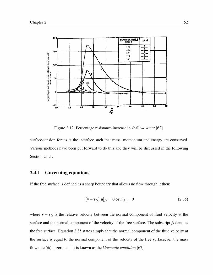
Chapter 2 52

Figure 2.12: Percentage resistance increase in shallow water [62].

surface- tension forces at the interface such that mass, momentum and energy are conserved.

Various methods have been put forward to do this and they will be discussed in the following

Section 2.4.1.

2.4.1 Governing equations

If the free surface is defined as a sharp boundary that allows no flow through it then;

[(v−vfs).n] f s = 0 or m f s = 0 (2.35)

where v− vfs is the relative velocity between the normal component of fluid velocity at the

surface and the normal component of the velocity of the free surface. The subscript fs denotes

the free surface. Equation 2.35 states simply that the normal component of the fluid velocity at

the surface is equal to the normal component of the velocity of the free surface, ie. the mass

flow rate (m) is zero, and it is known as the kinematic condition [67].

Chapter 2 53

The dynamic condition requires that the forces acting on the fluid at the free surface be in

equilibrium, such that there is momentum conservation at the free surface. The result is that the

normal forces on either side of the free surface are of equal magnitude and opposite direction,

and the tangential forces are of equal magnitude and direction. The interface conditions then

follow as:

(n.T )1 .n+sk =−(n.T )2 .n,

(n.T )1 .t− ∂s

∂t= (n.T )2 .t,

(n.T )1 .s− ∂s

∂s= (n.T )2 .s. (2.36)

where, s is the surface tension coefficient and k the local surface curvature. n, t and s are

unit vectors in a local orthogonal coordinate system (n, t, s), see Figure 2.13 [67]. The sur-

face tension is the force per unit length of a surface element and acts tangential to the free

surface. The subscripts 1 and 2 denote phases 1 and 2, which in this work are water and air

respectively. In two–dimensional space only one independent tangential vector exists, while in

three-dimensional space, two independent tangential vectors exist. Consequently, one tangen-

tial momentum jump will occur from Equation 2.36 in two dimensional space and two jumps

will occur for the three dimensional case.

The momentum interface conditions are a statement of continuity of stresses at a fluid boundary.

For an infinitesimally small surface element, the tangential components of the surface tension

forces cancel out when s = const and the normal component can be expressed as a local force

that results in a pressure jump across the surface [93].

Surface tension is a thermodynamic property of a liquid that depends on the temperature and

other state variables such as chemical composition and surface cleanliness. If it is assumed that

the temperature differences are small, then the temperature dependence of s can be linearised

so that ∂s

∂T is constant.

Chapter 2 54

Figure 2.13: A description of boundary conditions at the free surface [67].

In many applications the shear stress at the free surface can be neglected by assuming that, for

instance, the wind is negligible [67]. However, as has already been stated, the location of the

free surface is not known in advance and must be calculated as part of the solution and it must

be done iteratively, greatly increasing the complexity of the task.

Clearly the implementation of these additional free surface boundary conditions is not a trivial

matter and various numerical approaches exist. They fall into two main categories: fixed-mesh

and moving-mesh; or interface capturing and interface tracking methods. It should be noted that

all numerical methods for free surface flows are developed under a specific set of conditions,

assumptions, and degrees of approximation. In this sense, like much of CFD, a truly general

purpose method is not available and so the most appropriate method must be selected for the

given problem [94]. The first fundamental choice to be made regarding the interface represen-

tation is whether the whole flow, including the front(s), is described by an interface tracking or

Chapter 2 55

interface capturing method [95].

Interface tracking methods: Conceptually, the simplest means of defining and tracking a

free surface is to construct a grid that is embedded in and moves with the fluid. Many finite-

element methods use this approach and because the grid and fluid move together, the grid auto-

matically tracks free surfaces. The mesh is adapted dynamically in such a way that it is always

surface – conforming, whilst impermeable solid walls and free surfaces coincide with cell faces.

The location of the free surface is not known a priori. The free surface is treated as a sharp in-

terface and additional computational effort is required to keep this front sharp, by introducing

elements representing the front. These methods are best suited for well defined fronts that are

easily identifiable in the initial conditions. The initial, or unperturbed, free surface is used in

many interface tracking methods as a constant value from which any displacement of the free

surface relative to this can be calculated. It requires the introduction of a height function:

z = H(x,y, t) (2.37)

where, H is the change in height to the free surface, x and y are cartesian coordinates (in 2D)

and t is time. The kinematic condition 2.35 then describes the local change of the height, H:

∂H∂t

= uz−ux∂H∂x

−uu∂H∂y

(2.38)

This equation can be integrated in time to obtain the local height of the free surface. Some

commercial codes, such as TELEMAC, use this kind of approach where, at each point of the

mesh, the program calculates the depth of water and the two velocity components.

These methods and their application to free-surface flow have been described previously by

Zwart, Raithby & Raw [96] and The, Raithby & Stubley [97].

Chapter 2 56

Interface capturing methods: Here the flow and interface(s) are described in a Eulerian

way. In this approach the field equations are solved in an inflexible or stationary grid system

that extends beyond the free surface. The free surface and therefore the computational domain

are updated every time step. The major advantages of such an approach are its robustness for

problems containing complicated boundary geometries and the simplicity and relative ease with

which it can be implemented. These schemes can treat surfaces that undergo large distortions

and are ideal for the situation where an oar blade is placed just below the surface. The disad-

vantage of such methods is that their description of the boundary tends to be of lower order

than the tracking methods. This is because they average the flow properties of all fluid elements

in a given mesh cell, resulting in smoothing of variations and smearing of discontinuities [98].

Therefore high resolution grids are necessary to maintain a sharp front, which is something that

will be addressed in the grid generation process in Chapter 3.

The shape of the free surface is determined by computing the fraction of each near-interface

cell that is partially filled. The classical method is the marker-and-cell (MAC) approach first

proposed by Harlow & Welsh [99]. This scheme is based on a fixed Eulerian grid of control

volumes. The location of fluid within the grid is determined by a set of marker particles that

move with the fluid, but otherwise have no volume, mass or other properties. They serve as a

flow identification aid whereby fluid element trajectories can be tracked. Various modifications

and refinements to this fixed–grid method have since appeared [100, 101]; these mostly improve

the approximation of the free-surface boundary condition. The interface capturing method is

attractive because it can deal with complex phenomena like wave breaking; it is also readily

extendible to three-dimensional problems.

In 1981 the Volume of Fluid Method (VOF) of Hirt & Nichols [102] was introduced as an im-

provement to the MAC model. With the VOF method the interface is implicitly defined by the

fractional volume of a certain fluid in computational cells. For two–phase or two–fluid flows,

as is the case with the lake and air above it (neglecting any small particles in the water) the

Chapter 2 57

Figure 2.14: Volume fractions on a discrete mesh [88].

fractional volume can either be zero, or unity. A zero indicates the presence of one fluid and

a value of unity indicates the second fluid. On a computational mesh, volume fraction values

between these two limits indicate the presence of an interface and the value itself gives an in-

dication of the relative proportions occupying the cell volume (see Figure 2.14). Using volume

fractions is more economical than marker particles, as only one value needs to be accorded to

each mesh cell. So in addition to the conservation equations for mass and momentum (Equa-

tions 2.1 and 2.2) which are shared by both phases, two continuity equations need to be solved

for each phase. The continuity equation for the qth phase can be expressed as:

∂χq

∂t+ vi

∂χq

∂xi= 0 (2.39)

where the filled fraction of each control volume (CV), χ, is solved so that χ = 1 in filled CVs

and χ = 0 in empty CVs. Or, as is shown in Figure 2.14, it may contain some fraction between

zero and 1, for a partially filled cell. The fluid properties for each cell are adjusted according to

the local volume fraction. From continuity (Equation 2.39), one can show that the evolution of

Chapter 2 58

χ is governed by the transport equation:

∂χ

∂t+∇.(χv) = 0 (2.40)

A critical issue is the discretization of the convective term in Equation 2.40. Low-order schemes,

such as first order upwinding, smear the interface and introduce artificial mixing of the two flu-

ids. So higher order schemes are preferred in order to try and prevent overshoots or undershoots

of the surface location and maintain the condition that the filled fraction remains between zero

and 1 (0 ≤ χ ≤ 1) [67].

However, even with higher order methods, with the VOF method the free surface is not sharply

defined and is usually smeared over one, two or three cells. Therefore, it is important to have

local grid refinement for accurate resolution of the free surface in the area where 0≤ χ≤ 1. This

is an important consideration in the grid generation process. Additionally, various algorithms

have been developed to sharpen the interface between the two phases because of this smearing.

In the present work the geometric reconstruction method of Youngs [103] was employed.

All the variables including turbulent kinetic energy, k, dissipation rate, ε, Reynolds stresses, etc.,

are shared by the fluids throughout the domain and the volume fraction of each fluid in each

computational volume is tracked throughout the domain. For example density and viscosity are

attached to the two fluids and can also be expressed as a function of χ:

ρ = (1−χ)ρ1 +χρ2, (2.41)

µ = (1−χ)µ1 +χµ2, (2.42)

where, subscripts 1 and 2 correspond to the two phases, in this case they are water and air

respectively. If both fluids are treated in essence as a single fluid whose properties vary in space

according to the volume fraction of each phase then the interface itself does not need to be

treated as a boundary and so no boundary conditions need be prescribed on it. The interface of

Chapter 2 59

the free surface is simply the point at which the fluid properties change abruptly.

To reproduce the free surface sharply the convective flux along the cell faces is treated specially.

There must not be more fluid leaving a cell than is contained within it and the CV cannot accept

more fluid from a donor cell than there is space inside the acceptor cell. To control the cell face

values and compute the interface orientation correctly, the approximation of the cell face value

is managed by using a weighted upwind/downwind scheme which depends on the local Courant

Number (defined in Equation 2.9).

2.5 Moving mesh theory

A dynamic mesh model can be used to model flows where the boundaries of the domain move

rigidly with respect to each other. In Chapter 4 a moving mesh methodology is employed to in-

duce blade motion, where there is relative motion between stationary and rotating components

of the mesh. In Fluent this is known as sliding mesh motion and it will give rise to unsteady in-

teractions between the stationary and moving components. This section outlines moving mesh

theory which is utilised to model the fluid flow around the rowing oar blades in Chapter 4.

Incorporating moving objects exacerbates the situation and is an outstanding research topic in

CFD today [104]. The conservation equations outlined in Section 2.2 are modified in moving

zones to accommodate the flux variations due to the grid velocity. In integral form, the con-

servation equation for a general scalar, φ on an arbitrary control volume, V whose boundary is

moving can be written as:

∂

∂t

∫vρφdV +

∫∂V

ρφ(~v−~vg).d~A =∫

∂VD∇φ.d~A+

∫V

SφdV (2.43)

where ∂V represents the boundary of V , ~vg is the grid velocity of the moving mesh,~v is the flow

velocity vector, ~A is the area vector of the domain face, D is the diffusion coefficient and Sφ is

the source term of φ. A first order backward difference formula is used for the time derivative

Chapter 2 60

term (the first term) in Equation 2.43, such that:

ddt

∫V

ρφdV =(ρφV )n+1− (ρφV )n

Dt(2.44)

where, Dt is the time step size, the superscripts denote the time level, and V n+1 is evaluated as:

V n+1 = V n +dVdt

Dt (2.45)

with dVdt being the volume time derivative of the CV. The space conservation law [105] is em-

ployed to ensure that no volume surplus or deficit exists, when determining dVdt , such that:

dVdt

=∫

∂V~vg.d~A =

n f

∑j~vg, j.~A j (2.46)

where, n f is the number of faces on V and ~A j is the jth face area vector. The dot product~vg, j.~A j

on each control volume face is calculated from:

~vg, j.~A j =δVj

Dt(2.47)

where δVj is the volume swept out by the control volume face j over the time step Dt.

The motion of the moving zones is tracked relative to the stationary frame. The CV remains

constant, so that dVdt = 0 in Equation 2.45 and V n+1 =V n so that Equation 2.44 is now expressed

as:ddt

∫V

ρφdV =[(ρφ)n+1− (ρφ)n]V

Dt(2.48)

With the sliding mesh technique two or more cell zones are used and each cell zone is bounded

by at least one interface zone where it meets the opposing cell zone. The interface zone of

the adjacent cell zones are associated with one another to form a ‘grid interface’ and the two

cell zones move relative to one another along the grid interface in discrete steps. This situation

Chapter 2 61

Figure 2.15: Sliding mesh across a two–dimensional grid interface [88].

requires a means of computing the flux across the two non- conformal interface zones of each

grid interface.

To compute the interface flux, the intersection between the interface zones is determined at

each new time step. The resulting intersection produces one interior zone and a pair of wall

zones. The fluxes across the grid interface are computed using the faces resulting from the

intersection of the two interface zones, rather than from the interface zone faces themselves.

For each moving zone a translational velocity can be specified. Figure 2.15 shows how the

interface zones are composed of faces A- B and B- C, and faces D- E and E- F. The intersection of

these zones produces the faces a- d, d- b, b- e, etc. Faces produced in the region where the two cell

zones overlap (d- b, b- e, and e- c) are grouped to form an interior zone, while the remaining faces

(a- d and c- f) are paired up to form a periodic zone. To compute the flux across the interface

into cell IV, for example, face D- E is ignored and faces d- b and b- e are used instead, bringing

information into cell IV from cells I and III, respectively.

In Chapter 4 both the moving mesh models and the free surface theory will be employed to

produce an accurate model of the flow around moving rowing oar blades.

Chapter 2 62

2.6 Computational considerations

All CFD codes are centred around the numerical algorithms that tackle fluid flow problems.

In order to provide access to their solving power commercial CFD packages, such as Fluent,

include graphical user interfaces to input the problem parameters and to examine the results.

All codes contain three main elements: the preprocessor, the solver and the post–processor.

The preprocessor is employed to fully specify a CFD flow problem in a form suitable for the use

of the solver [68]. It is here that the geometry and the region of fluid to be analysed is defined.

This region of interest is called the computational domain and it is made up of a number of

discrete elements called the mesh (see Section 2.2.1); which is also generated at this stage. The

user needs to select the physical and chemical phenomena that are to be modelled and define

the properties of fluid acting on the domain. External constraints or boundary conditions (de-

scribed in Section 2.3.3), like pressure and velocity to implement realistic situations also need

to be specified.

The solver is a program that calculates the solution of the CFD problem. Here the govern-

ing equations are solved using the numerical techniques described in Section 2.2. CFD codes

contain discretization techniques suitable for the treatment of the key transport phenomena,

convection and diffusion as well as for the source terms and rate of change with respect to time.

An approximation of the unknown flow variables is obtained and a solution of the algebraic

equations is produced. As the equations are linear and tightly coupled an iterative approach

is required to solve them and careful control of the under–relaxation factors and time–steps is

required to ensure convergence. The purpose of the iterative process is to drive any residuals

towards zero. Also it is necessary to monitor force coefficients, such as lift and drag, to ensure

they reach stationary values.

A post–processor is used to produce visualisations and quantitatively process the results from

the solver. In contemporary CFD packages, the analysed flow phenomena can be presented in

vector plots or contour plots to display the trends of velocity, pressure, kinetic energy and other

Chapter 2 63

properties of the flow. The advances in computer technology over the past decades have enabled

CFD to be applied to complex flow fields and it has become a vital tool in research and design.

The accuracy of any numerical analysis is usually determined by the extent of computational

resources available for the project. Therefore, as well as describing the CFD techniques used, it

is also necessary to give some details of the computational resources.

All CFD simulations were run remotely on the Birmingham Environment for Academic Re-

search (BlueBEAR), a high performance computer cluster at the University of Birmingham,

UK. Typically, the simulations would be run over four dual–processor, dual-core nodes and the

nodes had 8 GB of memory. The nodes were connected through a low latency Infiniband inter-

connect (MPI latency < 7µs). The processors determine the speed of the solution and in this

case it was possible to run a number of simulations remotely at the same time using different

nodes (batch jobs).

For the more computationally demanding simulations parallel resources were employed. By

using processors in parallel it was possible to increase the speedup ratio, Sp (ratio of execution

time on a single processor to execution time for a parallel program on p processors). So that

S4 = 2 (i.e. with a parallel algorithm a speedup of two is achieved with four processors).

2.7 Summary

The background of CFD and the mathematical aspects of numerical simulation discussed in

this chapter provide the reader with basic knowledge for understanding the modelling process

adopted in the following three chapters.

In these later chapters, work focuses on the k− ε models and SST k−ω RANS models. This

is because the k− ε model is known to be robust and capable of providing a good preliminary

solution to a wide range of problems, while the SST k−ω model is known to produce more

accurate solutions for the kind of flow regime seen around rowing oar blades, but tends to be

Chapter 2 64

more unstable.

A description of free surface flow and meshing mesh techniques which will be employed in

Chapters 3 and 4, has been made. Discretization methods and the associated convergence and

stability issues which arise from the large system of non-linear algebraic equations in CFD

modelling, have also been discussed, as have the computational resources that were used for all

the simulations.

Chapter 3

Quasi–Static Investigation

3.1 Introduction

This chapter presents the first stage of the CFD modelling which was undertaken; establishing

the validity of the model. Testing of a CFD model should involve two phases: verification and

validation. Verification tests whether the numerical representation is an accurate solution of

the equations set up to define the physical situation and it is a purely numerical process [106].

So long as the theory withstands severe tests and is not superseded by another theory, it has

been corroborated or verified [107]. Validation is however the process of determining if a

mathematical model of a physical event represents the actual physical event with sufficient

accuracy [108]. Before a CFD model can be used as a stand alone computer based prediction of

events with confidence, it is good practice to undertake a thorough validation of the technique

against a published experimental data set.

Although all simulations in this chapter are quasi–static, layers of complexity are added as

the chapter progresses. The preliminary work outlined in Sections 3.2– 3.4 is concerned with

quarter scale blades and an assumption of a symmetry boundary condition is made at the free

surface. However, by Section 3.5 full size competition oar blades are modelled and comparison

65

Chapter 3 66

made to their quarter scale counterparts. In the final section of this chapter, Section 3.6, the free

surface interface between the water and air is modelled and a discussion is presented on how to

best model this boundary.

3.2 Experimental overview

Data from the CFD model presented here was compared with experimental measurements of

oar blade lift and drag forces obtained by Caplan & Gardner [23] in a water flume at the Uni-

versity of Birmingham, UK. The model blades were fabricated from 1.80 mm thick aluminium

sheet, which was of sufficient stiffness to allow the influence of blade bending to be disre-

garded. Several oar blade designs were tested, including the sweep version of the Big Blade

(Concept2 [51]) both with and without longitudinal curvature, a flat rectangular oar blade with

similar aspect ratio and projected area as the Big Blade and a Macon blade. The projected areas

of the blades (quarter scale and full size) are given in Table 3.1 and the blade designs are shown

in Figure 1.8. The model blades were also manufactured without a spine on the face of the

Table 3.1: Projected areas for the model quarter scale and full size oar blades tested.Blade Projected Area (m2)

Quarter Scale Full SizeFlat Rectangular Oar 0.007742 0.125Big Blade (flat) 0.007741 0.124Big Blade (curved) 0.007741 0.124Macon 0.006748 0.108

blade, as the current trend in oar design removes it (as discussed in Chapter 1). Each of the

blades was investigated at a range of discrete angles of attack, α, to the oncoming flow varying

between 0 ≤ α ≤ 180, where angle of attack is defined in Figure 3.1. The flume had a free

stream width and depth of 0.64 m and 0.15 m, respectively, and a length of 22 m. Due to the in-

herent wall resistance effects on the free stream velocity and the restrictions on the flume width

and height, it was considered necessary to use quarter scale models, which reduced the length

Chapter 3 67

Figure 3.1: View of the blade orientation.

of the blades to less than a quarter of the flume width. The blades were located 5 mm below

the air/water interface of the flume and were tested with a constant free stream velocity of 0.75

ms−1. The temperature of the water was 16C with a density and viscosity of 999 kgm−3 and

1.1545×10−3 kgs−1m−1 respectively.

To determine the lift and drag forces generated by the model oar blades, the forces acting both

normal and tangential to the chord line of the blade were measured. To achieve this calibrated

outputs from five strain gauge bridges were used and the voltage output from all of the gauges

were converted into moments about each bridge. Data from the strain gauges was sampled at

a frequency of 2500 Hz, for a period of 15 seconds and four measurements were taken at each

angle. The data collected during each 15 second period was averaged to provide a mean voltage

for each strain gauge, at each angle and from this the lift (FL) and drag forces (FD) for each angle

were calculated. The dimensionless force coefficients were then determined from Equation 1.3

by substituting these lift and drag forces, along with the projected areas of the oar blades given

in Table 3.1, and the measured fluid velocity.

Although no experiment is perfect, with errors inherent, any well designed experiment strives

Chapter 3 68

to keep them to a minimum. The percentage error that was reported was less than 10% at all

angles for each of the four blades tested [25]. Although the reported error is relatively small it

is important to remember these errors do exist, when comparing these measured values to any

CFD predictions, or indeed to on water measurements.

3.3 CFD methodology

The methodology described in this section adheres to a set routine common to any good CFD

investigation. The first step is to describe the problem in terms of its geometry and boundary

conditions; to set up the computational domain. This domain was defined in the preprocessor

Gambit (ANSYS, Inc., USA) and divided into sub–domains making up the mesh. From here

the mesh was exported into the processor, Fluent V6.3, where the models and type of simula-

tion were defined and solved. The theoretical basis to all of the turbulence models used was

described in Chapter 2 in detail. Once the solution had been deemed to converge then postpro-

cessing was carried out, producing numerical and visual outputs.

3.3.1 Geometry

The geometry of the simulation was dictated by a combination of the experimental setup of the

water flume used for the quarter scale measurements and computational efficiency. Figure 3.2

defines the layout and dimensions of the modelled domain which represented the experimental

flume used for the quarter scale measurements. It had the same width and depth as the ex-

perimental flume, but its length was reduced from 22 m to 4.5 m, to minimise computational

expense, since it was observed that the flow had recovered to a fully developed flow before

outlet, downstream of the blade. To illustrate this velocity profiles showing the variation of

velocity magnitude along the horizontal length of the flume (x–direction) are plotted in Fig-

ure 3.3. These profiles are taken from a CFD simulation on a flat rectangular oar held at 90

Chapter 3 69

Figure 3.2: Dimensions of the computational domain in millimetres.

to the free stream, but is representative of conditions in the flume for all blades at all angles.

At inlet and outlet the velocity is comparable, confirming that the flow has fully recovered by

outlet. It can also be seen that after the water comes in contact with the blade, indicted by the

downstream location in Figure 3.3, there is a significant change in the velocity magnitude of

the flow, as would be expected. The model oar blade will cause a blockage in the water flume,

if its size becomes significant relative to the cross–section of the flume it can distort the flow

over and around the model. The ratio between the model projected area and the channel area

is called the blockage ratio; when the blade is at 90 (when the greatest blockage is seen) this

ratio for the flat rectangular oar is 8%. This is in the range (5%–10%) where distortion effects

are known to become significant [109]. The blockage effect is something that was not flagged

in the experiments and may well have an influence on the results and especially at larger angles

of attack.

3.3.2 Mesh

As a number of blade angles of attack were investigated it was necessary to create an inner

cylindrical mesh containing the blade, while a second outer mesh was also produced containing

Chapter 3 70

Figure 3.3: Development of velocity magnitude along the length of the flume (x–axis). Inlet,a location downstream of the blade and outlet are plotted. Velocity magnitude reduces down-stream of the blade, but it is shown to recover by outlet.

the rest of the flume. The inner mesh was connected to the outer mesh using the non-conformal

mesh interfaces within Fluent. This approach allowed the inner cylindrical mesh containing the

blade to be rotated to provide the desired blade angle.

The mesh used in CFD can have a dramatic effect on the accuracy of the solution, and so an

important consideration for CFD is that of mesh quality [110]. The computational stability

and accuracy of the CFD calculation can be compromised if the mesh is not designed properly.

Thus, a systematic method of assessing the accuracy of a mesh by way of a mesh dependency

study is needed. This ensures mesh structures are developed to reduce mesh dependency to a

minimum without compromising the finite computing resource and/or incurring large computa-

tional expense.

It is first important to logically identify the areas where most resolution is required. In the case

of rowing oar blades presented here, the inner mesh is where the wake will form and develop.

Chapter 3 71

Therefore, the dependency study will focus on the inner domain. Three inner meshes were

generated (coarse, medium and fine) using unstructured tetrahedral cells in Gambit. In order

to compare these meshes in a non-dimensional way y+ values (defined in Chapter 2) are used

along with the lift and drag coefficients at one angle of attack (45). This angle was chosen

as it was expected to induce separation and turbulent flow features that the mesh needed to be

able to capture accurately. Considering the curved Big Blade mesh as an example, the coarse

grid contained 169,039 cells and had a mean y+ value of 345.78, it had no near wall resolution.

With a y+ value of this magnitude, when the mesh is used in conjunction with the SST k−ω

model, it will not perform adequately as it is recommended that y+ is the range of y+ < 2 [88].

However, with an enhanced wall function it should still perform relatively well, although it is

approaching the upper end of what is acceptable. It was felt that it was more appropriate, how-

ever, to try and place the y+ value in a range where the benefits of the SST k−ω model may

be realised. Therefore, for the medium and fine grids size functions and inflation layers were

attached to the faces of the blade and oar shaft to concentrate cells in the near wall region. In

this case a fixed size function, which limits the length of mesh-element edges within a region

specified by the distance from an existing entity, was used. For the medium mesh a start size

of 3, growth rate of 1.14 and a size limit of 100 were set. This ensured that around the blade

a sufficient number of elements were present and as the edge of the inner domain was reached

they were significantly more spread out, as can be seen in Figure 3.4.

Inflation layers are used to grow layers of cells from the wall being able to capture near wall

phenomena such as turbulence and allow resolution of flow field effects with fewer cells than

would be required without them, it is a memory efficient way of making a finer mesh. The

inflation layer on the inner mesh is shown in Figure 3.5.

It was found that the difference in solutions for the lift and drag coefficients for a medium

and fine grid were less than 1%, when tested at an angle of 45. The three meshes tested are

summarised in Table 3.2. The medium mesh was used for all subsequent simulations. For the

Chapter 3 72

Table 3.2: Mesh dependency study results for Big Blade held at 45 to the free stream.Mesh Coarse Medium Fine

No. of cells 169,039 350,000 600,000CPU/time step 3.0s 6.0s 36.0sy+

mean 345.78 1.07 1.07CL 1.771 1.204 1.213CD 0.851 1.099 1.107

medium mesh, the first cell was 0.06 mm away from the blade, producing a mean y+ value

of 1.07. It was considered that the enhanced wall treatment and the SST k−ω models should

be able to model the near wall region with these y+ values [68]. Figure 3.6 shows the surface

mesh on the Big Blade and flat rectangular oar blade for the medium mesh. Due to the sharp

edges at the attachment location there is a concentration of cells in this area. The outer mesh

created was a 6.5 m ×0.64 m ×0.15 m rectangular box, with a cylinder of the same dimensions

as the inner mesh removed at 1 m from the inlet (shown in Figure 3.7). It contained structured

hexahedral cells which were generated by using the Cooper algorithm which sweeps the mesh

node patterns from the top to the bottom of the volume. The combined mesh size of both inner

and outer domains was 3.5×105 cells.

3.3.3 Boundary conditions

Figure 3.8 indicates the type of boundary conditions and their positions. The velocity at the

inlet (marked ‘Velocity Inlet’) in Figure 3.8 is the velocity magnitude of the water in the flume

(a value of 0.75 ms−1 was used to match that from experimental data [22, 23]). At the boundary

marked ‘Outflow’ in Figure 3.8, a pressure outlet boundary condition was used. Here, as it is

incompressible flow, it takes the value 0.0 Pa to limit rounding errors. At the sides and bottom

of the domain and on both sides of the thin wall used to model the oar blade, ‘wall’ boundary

conditions the no–slip condition for what were smooth walls. For the standard k− ε model, a

law of the wall is used, which is used to specify the values of velocity, turbulent kinetic energy

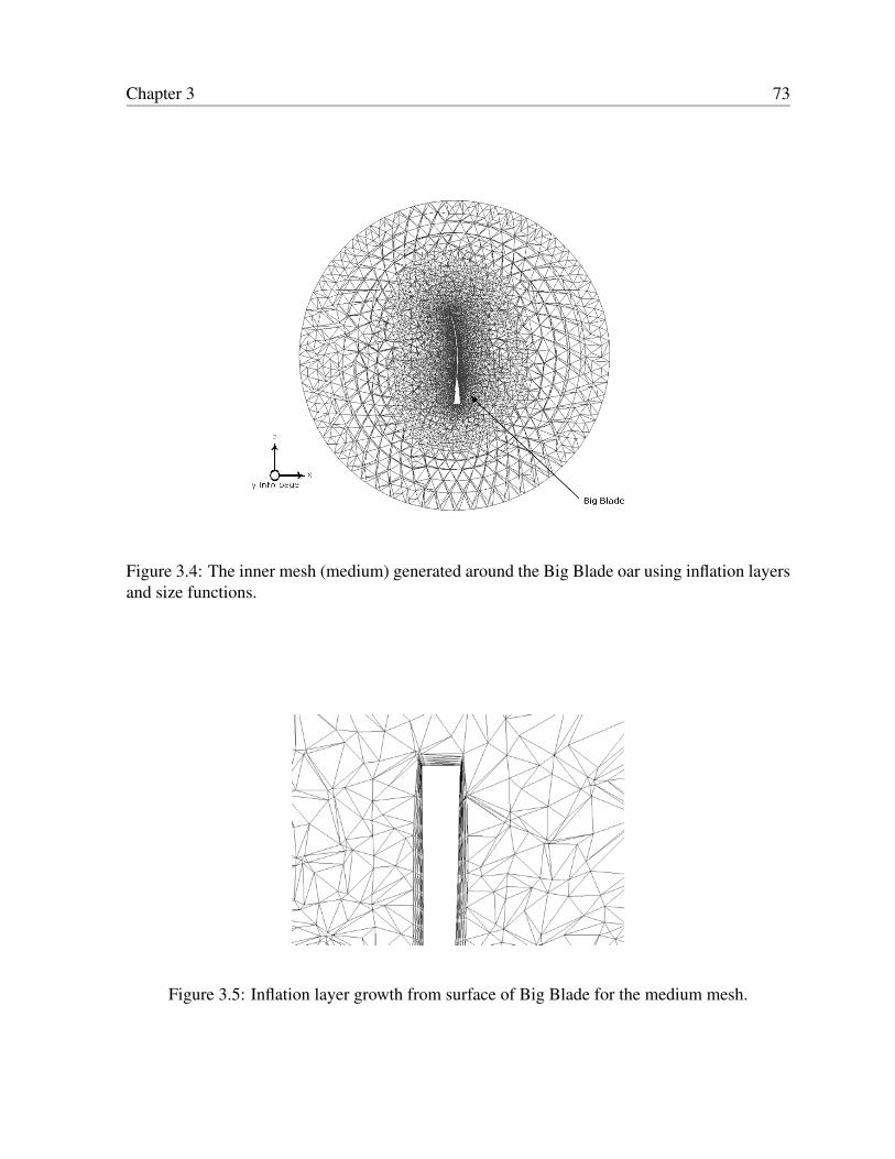
Chapter 3 73

Figure 3.4: The inner mesh (medium) generated around the Big Blade oar using inflation layersand size functions.

Figure 3.5: Inflation layer growth from surface of Big Blade for the medium mesh.

Chapter 3 74

Figure 3.6: Surface mesh of (a) Big Blade oar (b) flat rectangular oar of same projected area asthe Big Blade.

Chapter 3 75

Figure 3.7: The outer mesh generated for the Big Blade. The inner and outer meshes are unitedthrough a non–conformal interface.

and dissipation rate at the centre of the wall–adjacent cell; details of which can be found in

Chapter 2. In this application, the so- called enhanced wall treatment in Fluent were used. For

the SST k−ω model, the complexity of the model lies in its treatment of the near- wall region

and is described in detail in Chapter 2.

Finally, at the upper (high–y) boundary to the domain, the water surface, a symmetry boundary

condition was used. These boundaries are usually intended to allow the inherent symmetry in

both the geometry and flow within a domain to be used to the modeler’s advantage, by modelling

only part of the domain. However, in this application, it was chosen because it provides a closer

approximation to an immovable free surface than a slip wall condition.

Clearly, artificially constraining the flow in this way at the upper boundary is quite different from

the physical situation, especially considering the proximity of the blade to the free surface. It

was used as a preliminary approximation to the actual situation. The reasoning for this was that

the symmetry approximation substantially reduces computational effort compared with using a

Chapter 3 76

multi-phase model to model the water-air interface. As a result it was possible to carry out a

greater number of simulations. Further, a previous study has found good agreement between

CFD predictions and experimental data without modelling the free surface [30]. The inclusion

of the more complex situation that includes a free surface is detailed in Section 3.6 and the

results compared with this symmetry boundary condition.

Figure 3.8: Boundary conditions of computational domain.

3.3.4 Modelling procedure

All simulations were carried out using Fluent V6.3 [88]. At the time the research was conducted

this was the latest release of the software. Fluent is one of the current market leaders for com-

mercial ‘off-the-shelf’ CFD packages [111].

Different turbulent models and discretization schemes were investigated to see how effective

each of them was at modelling the flow. The k− ε model [81] with enhanced wall treat-

ment [112] was used initially as it is known to be more robust and applicable to a wide range of

flows [88]. The enhanced wall treatment formulates the law–of–the wall as a single wall law for

the entire wall region (laminar sublayer, buffer region and fully–turbulent outer region). This

is achieved by blending linear (laminar) and logarithmic (turbulent) laws–of–the–wall using a

function suggested by Kader [112]. The SST k−ω model [90] was also used as comparison,

Chapter 3 77

Figure 3.9: Convergence of residuals.

this is a more recent model that is known to be more accurate for this kind of flow regime. Both

of these models have been discussed in detail in Chapter 2. Additionally both first and second

order upwind discretization schemes were investigated, although it would be expected that the

second order schemes would provide the more accurate solution.

At greater angles of attack where separation and transient instability was likely to occur, that is

for 45 ≤ α ≤ 135, unsteady simulations were carried out to allow the unsteady phenomena

present at these angles to be investigated further. At the remaining lesser angles of attack, where

flow was known to remain attached to the back of the oar blade, a steady state simulation was

used. The PISO [113] algorithm was selected as the discretization scheme because it provides

a more stable calculation in transient simulations than the SIMPLE [37] or SIMPLEC [114]

alternatives [88]. The residence time, or the time for a given fluid particle to pass through the

Chapter 3 78

domain can be calculated using:

Tr =LV

(3.1)

where, L is the length of the domain and V is the velocity of a fluid particle. So that Tr is 6.67 s

and choosing a suitably small time step size of 1×10−4 s ensured that the transient flow features

occurring at this time scale, or greater, could be captured. It was felt that the time step size of

1×10−4 s was sufficiently small to capture the bulk of the transient behaviour. However, this is

by no means a certainty and further tests would be needed to ascertain that this time step size is

appropriate, although they have not been carried out in the present work. The simulations were

run until the solutions of lift and drag coefficients stopped varying by more than 0.01% and

all other residuals were monitored to ensure they too had fallen below acceptable convergence

levels. By plotting the residuals (Figure 3.9) for a given simulation it can be seen that the

solution has converged, and none of the values are changing by more than 0.01%.

3.4 Results and discussion

The primary measure of accuracy between experimental (measured) and CFD (predicted) re-

sults was the ability of the CFD models to predict the lift and drag coefficients at a number of

angles of attack. Secondary to this were flow visualisations, which although extremely useful

in gaining fluid dynamic insight, can only be compared qualitatively to other theoretical simu-

lations, as limited photographic evidence was available from the experimental work.

In Figures 3.12–3.21 lift and drag coefficients for the four oar blades are plotted. In general

the trends that were seen were similar for all four blades, and for the measured and predicted

results. An angle of attack of less than 90 indicated that the leading edge of the oar blade was

the tip of the blade, and an angle of attack greater than 90 in turn indicated that the leading

edge was the shaft end of the oar blade.

Drag coefficient was seen to increase with angle of attack until it reached a maximum at 90.

Chapter 3 79

As the angle of attack increased further, CD decreased towards zero.

Lift coefficient increased with angle of attack until a maximum was reached at approximately

45, and reduced to zero at 90. As the angle of attack continued to increase, with the leading

edge having changed to the shaft end of the blade, CL, decreased to a minimum at about 135.

As the angle of attack increased further, CL once again returned to zero. Although the lift co-

efficient is negative at angles greater than 90 this change in sign indicates that the direction of

the force generated by the oar blade changed direction.

These observations, from the examination of the numerical data, can be confirmed and rein-

forced through the use of visualisations. Contours of velocity magnitude (Figure 3.10a) and

pressure coefficient (Figure 3.10b) at a number of angles of attack were plotted (although this

plot is of the Big Blade, the principles hold true for the other blades as well). When the blade

is held at 20 to the free stream there is no, or very little turbulent wake produced, as shown in

Figure 3.10a, indicating a low drag coefficient. It can be seen in Figure 3.10b that, much like an

hydrofoil, there is high pressure on the lower surface of the blade and low pressure on its upper

surface; this pressure differential will induce lift. As the upward component of pressure on the

bottom of the blade increases (red indicating high pressure) the lift will increase. As the angle

of attack increases to 45 lift reaches its maximum and the turbulent wake behind the blade has

formed; indicating an increase in drag. Between 45–90 the lift starts to decrease, until at 90

it is at zero, with the component of low pressure on the upper surface of the blade dominating

over the high pressure on the lower surface. At the same time drag continues to increase, with

the turbulent structures in the wake of the blade becoming more pronounced. Figure 3.11 shows

an instantaneous visualisation using flow lines, originating upstream of the blade, for the Big

Blade held at 45 and 90 to the flow. It is clear that, as the flow separates, a wake is formed

behind the blade and there is also some counter rotation. The imbalance between this large area

of low pressure just behind the blade, and the small area of high pressure at the front of the

blade is the primary cause of the large drag coefficients at angles approaching stall. These

Chapter 3 80

Figure 3.10: Contours of (a) velocity magnitude (b) pressure coefficient at 20, 45, 70 and90.

Figure 3.11: Path lines released upstream of a Big Blade held at (a) 45 (b) 90 to the freestream flow. Separation is induced over the upper and lower surfaces of the blade in (a) and (b).Stall is seen in (b).

Chapter 3 81

Figure 3.12: Effect of turbulence model on the variation of lift coefficient with angle of attackfor a flat rectangular oar.

trends in lift and drag coefficient variation were observed, in general, for each of the four blades

investigated, although some discussion on their differences is made in Section 3.4.5.

3.4.1 Flat rectangular oar blade

The simplest of the oar blade designs used was the flat rectangular oar of equal shape and pro-

jected area to the Big Blade. Comparison was made between the measured experimental data

and the CFD predictions for each of the turbulence models and discretization schemes. These

data are shown in Figures 3.12 and 3.13 which compare the measured and predicted lift and

drag coefficients respectively for this flat rectangular oar blade plotted against angle of attack.

For both lift and drag coefficient, with this simple flat rectangular oar, the SST k−ω model

showed the best correlation for both coefficients. Also, as would be expected, the second order

scheme performed better than the first order scheme for both models. There was a slight over–

Chapter 3 82

Figure 3.13: Effect of turbulence model on the variation of drag coefficient with angle of attackfor a flat rectangular oar.

prediction of the values for lift and drag coefficient by the CFD model. For both computed lift

and drag coefficients a similar trend as the experimental data was found, and there was good

correlation between computed and experimental data for lift, but it was not as good for drag.

Table 3.3 summarises the absolute differences in the values of lift and drag coefficient for the

flat rectangular oar between CFD predicted values and experimental data using the second order

SST k−ω model. This indicates that lift is predicted, in absolute terms, to at least within 0.49

of the experimental result, and drag at least to within 0.60. The disparity between measured

and predicted data for drag may possibly be attributed in part to the top of the flume being

designated a symmetry boundary for the CFD simulations, rather than a free surface boundary

between water and air. However, since the match in lift appears not to be adversely affected

by the omission, it was doubtful that this was wholly the cause. The error in the experimental

measurements will also be a factor, however, as discussed above, this error was relatively small.

To highlight what a 10% error is in terms of the results for the flat rectangular oar, error bars

Chapter 3 83

Table 3.3: Absolute differences between experimental values and CFD values of lift and dragcoefficients, for quarter scale flat rectangular oar.

Angle (deg) Absolute difference in CL Absolute difference in CD

0 0.02 0.0420 0.40 0.2445 0.15 0.2070 0.09 0.2990 0.01 0.60

115 0.26 0.46135 0.30 0.27160 0.49 0.21180 0.03 0.03

(of 10%) are introduced in a plot of experimental and predicted lift and drag coefficients (Fig-

ure 3.14), where the Coppel et al. values of lift and drag coefficient are for the SST k−ω 2nd

order model.

Of the angles investigated, there are significant discrepancies in lift between experimental mea-

surement and the CFD predictions at 20 (0.40) and 160 (0.49). This is an important observa-

tion as any errors incurred here will influence the results of Chapters 4 and 5. It is evident from

Figure 3.14 that the experimental error plays a part, but the remainder of error is introduced

from the CFD modelling. The residuals were plotted to ensure they had dropped below accept-

able levels (0.01%) as indicated in Figure 3.9. It may be that the nature of the flow conditions

at these angles (highly turbulent, with separated flow regimes) are such that a RANS approach

is simply not sufficient. To approximate the turbulent behaviour more realistically it may be

necessary to use a LES (large eddy simulation), where large eddies are resolved directly, while

small eddies are modelled. Or DES (detached eddy simulation) which combines RANS and

LES by using a RANS model in the near–wall region while in the large separate flow regions

LES is used. To extend the research to include this level of prediction would require large

amounts of computer resources and is outside the scope of the current research.

Chapter 3 84

Figure 3.14: Experimental (with 10% error bar) and CFD predicted lift and drag coefficientsfor a flat rectangular oar.

3.4.2 Flat Big Blade

The next stage was to take an oar blade with the same planform shape as a typical oar blade – the

Big Blade, but with no curvature on the blade. Firstly the inclusion of an attachment to the oar

blade was investigated. Using the SST k−ω model with second order discretization a flat Big

Blade, with and without an attachment, was investigated. Figure 3.15 displays the surface mesh

on the flat Big Blade with and without an attachment. Looking at the drag coefficient, the results

which are shown in Figure 3.16, it can be seen that the inclusion of an attachment to the blade

improved the results by a small amount. This would suggest that the flow regimes developing

around the attachment to the oar blade have a small effect on the hydrodynamic properties of

the blade but choice of turbulence model and discretization scheme are more significant factors.

However, for completeness all subsequent simulations included an attachment to the oar blade.

Figures 3.17 and 3.18 compare the lift and drag coefficients respectively for the flat Big Blade

which again showed good correlation to the experimental results with the SST k−ω model with

second order discretization again showing the best correlation.

Chapter 3 85

Figure 3.15: Surface mesh of a flat Big Blade (a) with (b) without a shaft attachment.

Figure 3.16: Effect of inclusion of attachment on the prediction of drag coefficient for a flat BigBlade.

Chapter 3 86

Figure 3.17: Effect of turbulence model on the variation of lift coefficient with angle of attackfor a flat Big Blade oar.

Figure 3.18: Effect of turbulence model on the variation of drag coefficient with angle of attackfor a flat Big Blade oar.

Chapter 3 87

3.4.3 Big Blade

The next step was to add longitudinal curvature to the Big Blade blade as well as an attachment.

Again comparing the lift and drag coefficients for this blade (Figures 3.19 and 3.20) it can be

seen that good correlation to the experimental results was seen, with the SST k−ω second

order model proving the most capable at providing numerically accurate results. Table 3.4

Table 3.4: Absolute differences between experimental values and CFD values of lift and dragcoefficients, for quarter scale Big Blade with longitudinal curvature.

Angle (deg) Absolute difference in CL Absolute difference in CD

0 0.03 0.1220 0.03 0.1645 0.03 0.0970 0.04 0.0590 0.02 0.27115 0.1 0.34135 0.11 0.27160 0.14 0.01180 0.07 0.07

summarises the absolute differences in the values of lift and drag coefficient for the Big Blade

between CFD predicted values and experimental data. This indicates that lift is predicted, in

absolute terms, to at least within 0.14 of the experimental result, and drag at least to within 0.34.

3.4.4 Macon

The final blade design that was investigated was the Macon blade. This blade was the most

popular design from the 1950s until it was superseded by the Big Blade, which revolutionised

the market in the 1990s. Unlike the Big Blade the Macon is symmetrical and has a smaller

projected blade surface area (see Table 3.1). The development in oar blade design is discussed

in detail in Chapter 1.

The same procedure for modelling the flow around the blade was followed as before. For the

Chapter 3 88

Figure 3.19: Effect of turbulence model on the variation of lift coefficient with angle of attackfor a Big Blade oar.

Figure 3.20: Effect of turbulence model on the variation of drag coefficient with angle of attackfor a Big Blade oar.

Chapter 3 89

Figure 3.21: Experimental and CFD predictions of lift and drag coefficient with angle of attackfor a Macon oar.

Macon blade Figure 3.21 compares the CFD model with the experimental values of lift and

drag coefficient. Only the results of the second order SST k−ω model are shown as again they

showed the closest correlation to the experimental results.

Table 3.5 summarises the absolute differences in the values of lift and drag coefficient for the

Macon oar blade between CFD predicted values using the SST k−ω second order model and

experimental data. This indicates that lift is predicted, in absolute terms, to at least within 0.42

of the experimental result, and drag at least to within 0.18.

3.4.5 Comparison of blade designs

So far each blade has been considered in isolation, it is useful, however, to also compare between

blade designs and to observe the differences in them. The general fluid dynamic behaviour of

an oar blade at the angles of attack experienced during rowing has already been described at the

beginning of this chapter. The shape of the lift and drag curves has been discussed, however for

each blade there are some significant differences in these curves.

Chapter 3 90

Table 3.5: Absolute differences between experimental values and CFD values of lift and dragcoefficients, for quarter scale Macon blade.

Angle (degrees) Absolute difference in CL Absolute difference in CD

0 0.02 0.0420 0.06 0.1845 0.25 0.1570 0.14 0.0890 0.08 0.12115 0.04 0.02135 0.02 0.18160 0.42 0.16180 0.13 0.03

For each of the comparisons below, the SST k−ω model with 2nd order discretization was used.

Firstly, a comparison of the lift and drag coefficients of the flat rectangular oar blade and the

flat Big Blade is shown in Figure 3.22. It can be seen that although CL and CD are similar,

for the rectangular oar CL is elevated at 20–45 and 135–160. The drag coefficient is also

quite significantly greater for the flat rectangular oar. The increase in lift may be explained by

low aspect wing theory, whereby the straight edge helps to increase the magnitude of lateral

edge vortices through assisting in maintaining the attachment of the fluid flow to the back of the

blade. The Big Blade design, where the width of the blade reduces as the fluid flows from tip

to shaft, is a less effective method of generating lateral edge vortices, which has the effect of

reducing the lift.

In Figure 3.23 the effect of adding curvature to the Big Blade oar is investigated. It is expected

that by adding curvature circulation around the blade would increase; thereby increasing lift.

At angles greater than 90 the curved blade is able to generate lift more effectively than the flat

blade. For the Big Blade at these angles of attack the blade begins to resemble a delta wing,

where the distance between the two edges at any point along their longitudinal axis increases

from leading to trailing edge. This will result in stronger vortices developing along the top and

the bottom edges [63], which ensures that the fluid flow remains attached to the back of the

Chapter 3 91

Figure 3.22: Lift (x) and drag () coefficients are compared for the flat rectangular (—) and flatBig Blade (- -) oars. The SST k−ω 2nd order model was used for comparison.

Figure 3.23: Lift (x) and drag () coefficients are compared for the curved Big Blade (—) andflat Big Blade (- -) oars. The SST k−ω 2nd order model was used for comparison.

Chapter 3 92

Figure 3.24: Lift (x) and drag () coefficients are compared for the curved Big Blade (—) andMacon (- -) oars. The SST k−ω 2nd order model was used for comparison.

blade for longer, resulting in more lift being produced, as is seen between 135–160. At angles

less than 90 however, this trend is not observed, and the lift coefficients for both blades are

similar. Drag coefficient was found to be lower for the curved Big Blade above angles of 90 as

well.

Finally, the curved Big Blade and Macon blades were compared as shown in Figure 3.24. Since

the introduction of the Big Blade in 1991, performances have improved, suggesting an increase

in propulsive efficiency between the Big Blade and Macon blade designs [24, 50]. It can be

seen that between 45–70 and 115–180 that the Macon generates less lift than the Big Blade

oar. Drag coefficient is also significantly reduced for the Big Blade over the Macon blade. It has

been suggested [22, 25] that the improvements in propulsive efficiency are attributed mainly to

the smaller projected area of the Macon blade.

Chapter 3 93

3.5 Extension to full size

In Sections 3.2 – 3.4 only quarter scale oar blades were considered in the CFD analysis this

is because scale model data is also the only experimental data available in literature, as both

Caplan & Gardner [22, 23] and Barre & Kobus [31] use scale models; the former quarter scale

and the latter 0.7 scale.

The results presented in the previous sections have shown that the CFD models were capable

of producing an accurate simulation of the prevailing conditions of the flow in the experimental

flume. Lift and drag coefficients were compared and they corresponded to within an acceptable

level of accuracy.

Nevertheless, ideally all investigations would involve full scale apparatus to predict how identi-

cal copies of the equipment would perform under the same conditions. Such full size tests are,

in most cases, prohibitively expensive and often not feasible. The alternative then is to perform

experiments on small scale models with the resulting problem that measurements must then be

extrapolated to full-scale using dimensional analysis. Further, these small scale models do not

always simulate the behaviour of the full-scale case accurately due to necessary compromises

made in simulating actual full-scale conditions, and also with measuring instruments that are

not completely free from errors [37].

In the experiments of Caplan & Gardner [22, 23] it was necessary to scale down the blades to

a quarter scale, as they were constrained by physical limitations on the flume size and maxi-

mal flume velocity. This combination of constraints caused a compromise when a dimensional

analysis was undertaken.

3.5.1 Methods

With any fluid dynamics test requiring the use of scaled models, a dimensional analysis must

be performed to ensure actual full size conditions are being modelled [115], to do this it is

Chapter 3 94

necessary to ensure adherence to both geometric and dynamic similarity. As the model blades’

dimensions were reduced proportionally from the full size blades to the scaled models, geomet-

ric similarity was met. A ratio of 1 : 4 was chosen for the length scale, which in terms of the

characteristic length, L, is:

Lm =14

Lp (3.2)

where, the subscripts m and p represent model blade and prototype blade, respectively. It was

also necessary to match the non-dimensional Reynolds number, Re, for the model and prototype

blades. Reynolds number is used to quantify the relative importance of inertial and viscous

forces in a given flow, and was defined in Equation 2.4. If the model and prototype Reynolds

numbers are equated:

Rem = Rep

ρvmLm

µ=

ρvpLp

µ(3.3)

vm

vp=

Lp

Lm

Substituting equation 3.2 leads to:

vm = 4vp (3.4)

If the prototype relative blade velocity vp is 5 ms−1, then it follows from Equation 3.4 that the

required model relative blade velocity in the flume, vm, is 20 ms−1.

Since in rowing, relative blade-water velocity is expected to vary over the stroke between ap-

proximately 1 ms−1 and 5 ms−1 [11], a constant velocity of vp = 5 ms−1 [Re= 2.3×106] was

assumed, which is consistent with values seen early and late in the drive phase of the rowing

stroke [7]. Thus, for dynamic similarity, the model free stream velocity in the flume, vm, was

required to be 20 ms−1 [Re= 2.3×106]. Unfortunately, the experimental flume [22, 23] could

not be operated at this velocity, resulting in dynamic similarity not being met. To address this

Chapter 3 95

problem, Reynolds number dependence on the lift and drag coefficients for a flat rectangular oar

was investigated and it was found that with a flume velocity of above 0.7 ms−1 the coefficients

were independent of Reynolds number. Therefore, the resulting range of flume velocities that

showed negligible variation in the force coefficients was only in the range 0.7 – 0.85 ms−1. This

meant that if a fluid velocity of 0.75 ms−1 [Re= 8.8×104] was used, this should have been high

enough to overcome any influence of Reynolds number, but also low enough to ensure that the

boundary effects arising from the walls of the flume would not adversely influence the validity

of the results.

This idea of Reynolds number independence is corroborated in the literature by Munson et

al. [5] and Hartwanger & Bunt [3] who state that for a fully immersed bluff body, such as a flat

plate, in the range of Reynolds numbers considered, that a CD versus Re curve (drag coefficient,

and Reynolds number, respectively) will level off to a flat line, when 105 ≤ Re ≤ 107. Thus,

Reynolds number is not expected to be critical for objects that are fully submerged, provided

the flows are turbulent. Caplan & Gardner [22, 23] made the assumption that if this was true

for a flat rectangular oar, similar comparison could be made for rowing oar blades which only

have a shallow curve. However, it has also been found in recent work by Sliasas & Tullis [46]

that significant differences between rectangular plates of similar areas to quarter and full size

oar blades. They found that the full size plates had a 20% lower lift coefficient and a 30% lower

drag coefficient than quarter scale plates.

This section will therefore deal with testing this assumption, and to investigate the accuracy of

the previously published data from Caplan & Gardner [22, 23] in relation to full size oar blades.

It is appropriate to use the CFD model, since it has been previously validated by demonstrating

its accuracy in simulating the actual test conditions at quarter scale in Section 3.3.

For Caplan & Gardner’s [22, 23] assumption to be correct, force coefficients should remain

constant above a relative blade velocity of 0.75 ms−1. Therefore, their experimental values for

a quarter scale blade with a relative blade velocity of 0.75 ms−1 should match the quarter scale

Chapter 3 96

CFD values at 0.75 ms−1 and 20 ms−1 and the full size CFD values at 5.0 ms−1. In short,

the CFD solutions for the force coefficients for all three above CFD cases should be exactly

the same. Since the correlation between experimental and CFD coefficients for quarter scale

results at 0.75 ms−1 is already addressed in Sections 3.2–3.4, this investigation will be confined

to testing the hypothesis that the CFD results found in the present study are unchanging at 0.75

ms−1 and 20 ms−1 (quarter scale) and 5 ms−1 (full size).

As before all simulations were carried out using Fluent V6.3. The SST k−ω model was used

as the turbulence model with second order discretization as this has been found to be the most

accurate in simulating the flow over the oar blades at all angles.

The dimensions of the modelled computational domain were four times larger than the water

flume described in Section 3.2, and the blade corresponded to the dimensions of a typical full

size competition oar blade. The projected area of the full size blades used were detailed in

Table 3.1.

A mesh independency study was carried out on the full size blade to ensure high quality solu-

tions were being produced. For consistency the 45 Big Blade was used again to compare lift

and drag coefficients across three meshes (coarse, medium and fine). The coarse mesh consisted

of 169,039 cells, it did not have a inflation layer imposed on it and so a mean y+ value of 345.78

was produced. The medium mesh was generated with a focus on the generation of a inflation

layer, it had 359,476 cells and the mean normal distance of the first node from the wall was 0.06

mm, which produced a mean y+ value of 17.27. The fine mesh had 891,103 cells and the first

cell was 0.005 mm from the wall and the mean y+ was 1.53. As can be seen from Table 3.6 the

results from the coarse and medium mesh differ considerably, whereas the difference between

the medium and fine meshes is negligible. Thus, it can be argued that the medium mesh can be

used with confidence for subsequent simulations of different blade angles.

Chapter 3 97

Table 3.6: Mesh dependency study results for full size Big Blade held at 45 to the free stream.Mesh Coarse Medium Fine

No. of cells 169,039 359,476 891,103CPU/time step 3.0s 6.0s 36.0sy+

max 946.46 35.15 3.53y+

min 46.73 1.32 0.14y+

mean 345.78 17.27 1.53CL 1.77 1.03 1.04CD 0.851 0.817 0.821

3.5.2 Results and discussion

Figures 3.25 and 3.26 present the lift and drag coefficients, respectively, for the full scale CFD

model at the range of angles of attack tested for the Big Blade, using a free stream velocity of

5 ms−1. The quarter scale force coefficient profiles for a free stream velocity of 20 ms−1 and

0.75 ms−1 were also compared to test the validity of Caplan & Gardner’s [22, 23] assumption.

For their assumption to be correct, force coefficients should remain similar above a free stream

velocity of 0.75 ms−1.

If Figure 3.25 is examined, which presents the variation of lift coefficient with changing ve-

locity and angle of attack, it would seem that this assumption holds reasonably well for the

lift coefficients as there is little variation (see Table 3.7) between the quarter and full size val-

ues at the majority of angles. Although there is some reduction in the full scale values in the

115 ≤ α ≤ 180 range, which is in agreement to Sliasas & Tullis’ [46] findings. Comparing

the drag coefficients in Figure 3.26 and Table 3.7 of the full size blade with a velocity of 5 ms−1

and the quarter scale blade at 0.75 ms−1 it can be seen that at all angles the drag is greater at

quarter scale. This suggests some Reynolds number dependence between the two flow veloci-

ties, and therefore that force coefficients are dependent on flow velocity between 0.75 and 20

ms−1, which is confirmed by the disparity between quarter scale curves at velocities of 0.75 and

20 ms−1 in Figure 3.26. These differences are again corroborated in the literature by Sliasas &

Tullis [46] who found ≈ 30% reduction in drag at full scale for rectangular flat plates.

Chapter 3 98

Figure 3.25: Lift coefficient variation with angle of attack. Comparison is made between CFDsimulations of a quarter scale Big Blade at 0.75 ms−1, Re = 88×103; a full-size Big Blade at5 ms−1, Re = 2.3×106 and a quarter scale Big Blade at 20 ms−1, Re = 2.3×106.

Figure 3.26: Drag coefficient variation with angle of attack. Comparison is made between CFDsimulations of a quarter scale Big Blade at 0.75 ms−1, Re = 88×103; a full-size Big Blade at5 ms−1, Re = 2.3×106 and a quarter scale Big Blade at 20 ms−1, Re = 2.3×106.

Chapter 3 99

Tabl

e3.

7:A

bsol

ute

diff

eren

ces

inth

eva

lues

oflif

tan

ddr

agco

effic

ient

betw

een

CFD

sim

ulat

ions

with

mat

ched

Re

num

bers

(qua

rter

scal

e,v

=20

ms−

1an

dfu

llsc

ale

v=

5m

s−1 )a

ndC

FDsi

mul

atio

nsw

ithun

mat

ched

Re

num

bers

(qua

rter

scal

e,v

=0.

75m

s−1

and

full

scal

ev

=5

ms−

1 )for

aB

igB

lade

.A

ngle

Abs

olut

edi

ffer

ence

inC

LA

bsol

ute

diff

eren

cein

CD

mat

ched

Re

num

ber

unm

atch

edR

enu

mbe

rm

atch

edR

enu

mbe

run

mat

ched

Re

num

ber

1/4

scal

e20

ms−

1vs

.ful

lsiz

e5

ms−

11/

4sc

ale

0.75

ms−

1vs

.ful

lsiz

e5

ms−

11/

4sc

ale

20m

s−1

vs.f

ulls

ize

5m

s−1

1/4

scal

e0.

75m

s−1

vs.f

ulls

ize

5m

s−1

00.

000.

060.

010.

0420

0.17

0.21

0.03

0.13

450.

180.

080.

080.

2990

0.01

0.00

0.05

0.49

135

0.13

0.30

0.03

0.19

160

0.01

0.50

0.01

0.09

180

0.01

0.10

0.01

0.04

Chapter 3 100

The largest reduction in the drag coefficient is seen at 90, with a 35% difference between

the dynamically unmatched simulations of 0.75 ms−1 quarter scale, and the 5 ms−1 full scale

results, compared with only a 4% difference in the dynamically matched simulations (quarter

scale at 20 ms−1, and full scale at 5 ms−1). At 90 a large turbulent wake forms behind the

blade which causes form drag. This may be explained as follows; when Reynolds number is

large, the viscous forces, and therefore the energy dissipation, are relatively small compared

with the inertial forces and unsteady vortices will appear and interact with each other [112].

The reduction in drag may be due to the reduction in the size of the wake as the flow speed

increases, which effectively reduces the form drag. Additionally, having large angles of attack

will cause separation in both a curved and flat blade. The magnitude and exact nature of the

separation is dependent on the shape of the blade as well as its angle of attack.

Curvature of the blade will play an important role in the way drag is produced, since curvature

along with vorticity and pressure gradients, are important factors that govern the formation of

turbulence. Curvature can be significant in oar blades and can modify aspects of the flow in a

nontrivial fashion through the way it influences turbulence [116]. An oar blade possesses con-

cave curvature, which can lead to the generation of longitudinal (Taylor–Gortler) vortices [117].

These vortices amplify the large scale motions normal to the blade surface and because of the

new eddy structure the mixing across the boundary layer adjacent to the blade surface is en-

hanced, bringing high momentum fluid closer to the wall than with a normal flat boundary layer

(such is the case with a flat plate). This causes a significant increase in the skin friction, which

will have a direct influence on the drag.

It is also worth noting that the numerical mesh used for the full size simulations was different in

terms of the y+mean value (17.27 compared with 1.07 at quarter scale). However, given that com-

parable readings were made between Reynolds number matched quarter and full scale blades,

and that both sets of solutions were independent of the grids being used, it was evident that the

grid was not influencing the results.

Chapter 3 101

In summary, the discrepancy between quarter and full size predictions of drag coefficient in

Figure 3.26 may well be due to the assumption that drag coefficient is independent of Reynolds

number in the two unmatched models at flow velocities of 0.75 ms−1 and 5 ms−1, and may also

be due to the premise that an oar blade has similar fluid dynamic behaviour to a flat plate. When,

drag coefficients for two dynamically matched CFD models, which do account for Reynolds

number independence were compared, better agreement was seen. This would lead to the con-

clusion that it is important to have dynamic similarity and is in agreement to the current lit-

erature [46] which has found comparable results for flat rectangular plates of similar areas to

scaled and full size oar blades. Further improvement in the accuracy of the simulations would

also be required to draw any further conclusions.

3.6 Free surface ow

In the preceding sections of this chapter the upper boundary of the flume has been treated as

a symmetry condition. This type of approach may cause the flow to be artificially accelerated

which may influence the lift and drag coefficients. The blockage ratio (as described in Sec-

tion 3.3.1) will also be influencing the flow. It has been noted that using a symmetry condition

(or a rigid lid approach) simplifies the problem, as it does not allow the free surface to deform,

and it is more representative of the physical conditions to model this boundary as a free surface.

However, flows with free surfaces are an especially difficult class of flow to model. This is

because sharp fronts exist in multi-fluid or multi-phase flows, where fluid properties, such as

density and viscosity change rapidly. In the case of an oar blade used in rowing the two fronts

that interact with each other are air and water at the ‘free surface’. This subsequently increased

the magnitude of the computational requirements needed to undertake free surface modelling

and so influenced the number of simulations it was feasible to perform. So although the mod-

elling described in this chapter is a better representation of the physical conditions seen in the

Chapter 3 102

water flume, the work discussed in the preceding sections, undertaken without a free surface

may well be practically of more use when intending to carry out a large number of simulations.

The numerical basis of free surface techniques is described in Section 2.4.

3.6.1 Methods

The process of creating the CFD model is consistent with the previous routine described in

Section 3.3. Starting with the description of the geometry through to creating the mesh, setting

up the model and solving for the lift and drag coefficients.

Geometry

The geometry of the flume remained unchanged with the same length, width and depth as in

Section 3.3. The position of the blade within the flume was also in agreement to the previous

setup. However, with the addition of the free surface, a region of air above the flume needed to

be included for use with the VOF method. The height of this air portion should be large enough

to avoid any effect from the boundary condition at the top of the domain, yet small enough that

unnecessary computational expense is not incurred. Figure 3.27 shows the extension above the

flume, with the dashed line representing the set height of the free surface; which was 5 mm

above the blade and 150 mm from the base of the flume. The total height of the domain was

therefore increased to 300 mm. It is also important to ensure that the depth of the flume is great

enough to ensure no shadow effects are occurring, which may artificially influence the flow.

Blockage ratio, described in Section 3.3.1, is one way of determining if the bottom of the flume

is far enough away from the blade for it not to be an influencing factor. It is also prudent to

investigate the pressure variation over the flume depth.

Chapter 3 103

Figure 3.27: Side view of computational domain used for modelling the free surface.

Mesh

Unlike in the previous sections that did not model the free surface, with this more complex case

it is unsuitable to have a non–conformal interface boundary condition between the inner and

outer meshes. Inclusion of such an interface would increase, the already large computational

requirement, still further. This means that for each blade angle a separate mesh was required.

It was again important to ensure an accurate representation of the flow details around the blade,

so that a successful prediction of the turbulent flow away from the blade was produced and that

ultimately a good prediction of lift and drag coefficients would be made. It was also vital to

provide a finer grid near the air–water interface to capture the variations in the location of the

free surface. Figure 3.28 shows two of the grids that were investigated (‘fine’ and ‘medium’)

to simulate the 2D flat rectangular oar held at a 90 angle. The orientation is looking side on

to the flume along the length (x–direction). The fine grid was selected as it provided the most

resolution in the free surface region, as well as in the region downstream of the blade.

Chapter 3 104

Figure 3.28: Flat rectangular oar in 3D showing grid resolution in the free surface region (a)medium mesh (b) fine mesh.

Boundary Conditions

The boundary conditions applied to the domain are indicated in Figure 3.27. An open channel

was used to represent the water flume, with a mass flow at inlet and a pressure outlet. The mass

flow rate at inlet can be calculated for each phase from Equation 2.26. For the air phase it was

assumed that there was no wind and so the mass flow rate was zero. For the water phase A=

0.64×0.15 = 0.096 m2, and V = 0.75 ms−1, as in the previous experimental studies [22, 23].

This means that the water mass flow rate at inlet was 71 kgs−1.

At outlet the pressure was specified by the free surface level method where the free surface level

is specified by ylocal:

ylocal =−(~a.g) (3.5)

where ~a is the position vector of any point on the free surface, and g is the unit vector in the

direction of the force of gravity. It is assumed that there is a horizontal free surface that is

normal to the direction of gravity. The sides of the flume and the blade were designated as no

slip walls. These boundary conditions have been described in more detail in Section 2.3.

Chapter 3 105

Modelling procedure

All simulations were carried out using Fluent V6.3. A transient pressure based solver was used

with gravity switched on. It is important to have gravity in the correct sense as the free surface

is dependent on this. The VOF method with an explicit open channel flow scheme was used to

model the free surface with air and water, defined as phases 1 and 2 respectively.

The k−ε RNG turbulence model with enhanced wall functions was used. This model has known

advantages over the standard k−ε model when there is strong curvature in the stream lines [86].

It has been used extensively in literature for investigating two–phase flow [106, 118, 119, 120]

and so was deemed appropriate for this investigation (the RNG model is described in Sec-

tion 2.3). Further, as is noted in Chapter 4, this model provides similar results to the SST k−ω

model.

A second order discretization scheme was used, this was needed to improve the accuracy of the

solution, however higher order schemes have a tendency to reduce the stability of the solution.

Thus, Rhie-Chow’s interpolation [121] scheme was applied to overcome the ‘checkerboard’ ef-

fect on collocated unstaggered grids. ‘Checkerboarding’ is an undesirable effect in which the

momentum equations contain the pressure difference between two alternative grid points rather

than between adjacent ones. This implies that the pressure is taken from a coarser grid than one

that is actually employed. As well as diminishing the accuracy of the solution it has a more seri-

ous implication of zeroing out an oscillating pressure field. Thus, a highly nonuniform pressure

field would be treated as a uniform pressure field by the particular discretized form of the mo-

mentum equations. The standard Rhie-Chow procedure was used to avoid these checkerboard

oscillations. For a solution of the pressure from the momentum equations, a pressure correction

step was required. This is obtained from the fact that after each time step the continuity equation

will, in most cases, not be satisfied.

The PISO algorithm was used to calculate the pressure and velocity field. Beginning with

the boundary conditions the velocity and pressure gradients are calculated and the discretized

Chapter 3 106

momentum equations were solved. This gave the intermediate velocity field which is used to

calculate the uncorrected mass fluxed at the cell faces. After correcting the pressure field and

the boundary pressure the mass fluxes across the cell faces are corrected. After this the cell

velocities are updated.

A high resolution interface capturing (HRIC) scheme based on the compressive interface cap-

turing scheme for arbitrary meshes (CICSAM) [122] was used with the VOF approach. Small

values for under-relaxation factors (URF) are required for the stability of the solution using this

interpolation scheme, therefore a value of 0.7 was chosen.

A good indication as to how long the simulation should be run for depends on the residence

time; or the time it takes for a given particle to travel through the domain. The residence time

can be calculated from Equation 3.1. When the length of the water flume is 4.5 m and the

velocity of the flow is 0.75 ms−1 the residence time is 3.38 s. It was important to run the sim-

ulation for a number of residence times to ensure the solution reached convergence. It was also

necessary to monitor the convergence of lift and drag coefficients so that they too had reached

a stationary value. To ensure that the solution remains stable a small time step must be used,

especially when the simulation is first started. All the simulations were initially run with a time

step of 1×10−4 s which was gradually lowered after a few thousand iterations. The simulations

were run over several thousand integrations, until the values of lift and drag coefficient stopped

varying by more than 1%. The convergence history of the coefficients was monitored and is

shown for the drag coefficient of the Big Blade held at 90 in Figure 3.29. Since the type of

flow fields which are being modelled involve wake shedding which is highly transient and re-

quires of the order 2–5 s to establish; it can be appreciated how many time steps are required to

reach stationary values of lift and drag coefficient. The great care that has been taken to ensure

the stability of the solution and inhibit divergence highlights the complexity of the problem in

hand.

Chapter 3 107

Figure 3.29: CD convergence history for a Big Blade oar held at 90 to the free stream.

3.6.2 Results and discussion

Results are presented for two blades only, a flat rectangular oar and a Big Blade with curvature.

The large computational expense that was experienced with the free surface calculations war-

ranted fewer simulations being undertaken. The advantage of using the flat rectangular oar as

one of the cases was that could be investigated in both two – and three – dimensions, allowing a

preliminary study to be carried out in 2D before extending to the more computationally demand-

ing 3D. For the Big Blade it was only possible to consider a 3D situation given the curvature,

attachment and shape of the blade. This highlights the persistent 3D nature of any investigation

into rowing oar blades. It seemed logical, given the greater computational expense needed with

the inclusion of the free surface, rather than to investigate a large number of blade angles, as

was carried out as before, to look at only three angles for the three dimensional blades (45,

70 and 90) which were representative of different points in the rowing stroke. The results for

lift and drag coefficient are compared with the experimental [22, 23] and the ‘no free surface’

values from the earlier simulations.

Chapter 3 108

Figure 3.30: Visualisations of flow over a 2D flat rectangular oar blade at t= 0 s , t= 0.05 s,t= 15 s (VOF=0.5).

2D Flat rectangular oar blade

Initial simulations were undertaken using a two dimensional flat rectangular oar blade. Fig-

ure 3.30 shows a series of visualisations indicating the development of the flow over the blade.

The flow is from left to right along the length of the flume as if looking side on. It is possible to

see the significant flow structures which are produced, much like a breaking wave.

As most numerical procedures will introduce artificial diffusion leading to pronounced mass

conservation errors [123] a further check is needed to ensure continuity holds (m1 = ρAV = m2).

Therefore, mass flow rate at inlet and outlet were monitored and the mass imbalance was found

to be less than 0.1%. This is a numerical error, rather than one stemming from the finite volume

method, which by definition, will conserve mass.

3D Flat rectangular oar blade

Presented below in Figures 3.31 and 3.32 are the lift and drag coefficients respectively of the

flat rectangular oar in 3D held at three angles of attack to the free stream. CFD simulations with

and without a free surface are compared with the experimental results. It can be seen that for the

three angles investigated, the ‘no free surface’ case over–predicts the lift and drag coefficients,

while the free surface case under–predicts them. The differences with the experimental results

are as great for the no free surface case as with the free surface case.

Chapter 3 109

When there is no free surface, the pressure at the top boundary will tend to rise, because of the

presence of a ‘lid’ instead of a boundary which is allowed to deform. This may be attributing to

the spurious values of lift and drag coefficients seen in Figures 3.31 and 3.32. Another influence

is blockage ratio which although only around 8% could also be influencing the results, causing

an artificial representation of the flow.

In rowing, while the blade is completely submerged during a rowing stroke, it comes very close

to the surface (within a few millimetres) and can be compared to surface piercing bodies for this

reason. Hoerner [62] presented drag results of an investigation into a surface-piercing flat plate

normal to the flow. The phenomenon of ventilation, the presence of an air filled space usually

behind a bluff body, was illustrated in these experiments (Figure 2.11). For ventilation to occur

there must be a region of low pressure into which the air can be sucked. There must also be

a means of channelling this air into the low pressure area. The onset of ventilation coincides

with the decrease of wave drag. This implies that ventilation inhibits the motion of the fluid in

a wave and consequently a reduction in the transfer of momentum.

It would seem that the drag of bodies at, or near, a free surface is dominated by wave drag and

therefore preventing or minimising wave formation and inevitably reduces drag. As compared

with completely submerged bodies, those that pierce the free surface or, are at least very close

to it, tend to reduce the magnitude of the drag curve. The absolute differences in the free surface

and no free surface values compared to experimental measurement are presented in Table 3.8.

These absolute values along with the plots presented in Figures 3.31 and 3.32 corroborate Ho-

erner’s [62] findings which showed that bodies close to or piercing a surface tend to reduce the

drag and lift coefficients.

3D Big Blade

Presented in Figures 3.33 and 3.34 are the lift and drag coefficients of the Big Blade held at

three angles of attack to the free stream. CFD simulations with and without a free surface are

Chapter 3 110

Figure 3.31: Comparison of flat rectangular oar lift coefficient values for experimental resultsand CFD results with and without a free surface boundary.

Figure 3.32: Comparison of flat rectangular oar drag coefficient values for experimental resultsand CFD results with and without a free surface boundary.

Chapter 3 111

Table 3.8: Absolute differences between experimental values and CFD values (with and withouta free surface) of lift and drag coefficients, for 3D flat rectangular oar.

Angle No Free Surface Free SurfaceCL CD CL CD

45 0.14 0.20 0.24 0.2170 0.09 0.29 0.14 0.3690 0.001 0.60 0.01 0.19

compared with the experimental results. It can be seen that for the three angles investigated,

the free surface case under-predicts the lift and drag coefficients to a greater degree than the ‘no

free surface’ case. The absolute differences in the free surface and no free surface values com-

pared to experimental measurement are presented in Table 3.9. Again the onset of ventilation

downstream of the blade at the free surface (which is depicted in Figure 3.30) may be affecting

the results causing a low pressure area which reduces drag coefficient when compared to the no

free surface case. However, the CFD models perhaps exaggerate the effect of this ventilation

as the drag coefficient values are unnaturally low and much lower than the experimental values.

So although physically the ventilation behind the blade has been modelled by incorporating the

free surface into the models, the numerical prediction of lift and drag coefficients are not any

closer to the experimental values than they were with a symmetry boundary condition. Recall-

ing from Section 3.3.1 that the experimental results were in the range where blockage effects

become significant. This is likely to provide further distortion of the results that are seen here,

as the flow over and around the blade was also being influenced by the proximity of the wall to

the blade.

Table 3.9: Absolute differences between experimental values and CFD values (with and withouta free surface) of lift and drag coefficients, for a Big Blade.

Angle No Free Surface Free SurfaceCL CD CL CD

45 0.026 0.040 0.091 0.29070 0.040 0.070 0.052 0.25090 0.018 0.021 0.275 0.460

Chapter 3 112

Figure 3.33: Comparison of Big Blade lift coefficient values for experimental results and CFDresults with and without a free surface boundary.

3.7 Summary

This chapter has outlined the use of CFD in simulating fluid flow around a number of different

oar blade designs. By firstly using a published experimental data set on quarter scale blades as

a comparison, it was possible, using the CFD simulations, to replicate the findings to an accept-

able level of accuracy. The main flow measures were the lift and drag coefficients of the oar

blades, and it was found that these were sensitive to the choice of turbulence model. The use

of the SST k−ω turbulence model resulted in a better correlation to the measured experimental

data than the standard k− ε model. This was true for all of the four blades tested, at all angles

of attack. The SST k−ω model performed least well at angles of attack that approached the

stall condition, where a large amount of separation was induced. Here it was necessary to use

an unsteady model to capture the unsteadiness as time progressed.

The CFD model was used to extend the current research to investigate full size oar blades. The

previous experimental work had been constrained by the inability to match dynamic similarity

Chapter 3 113

Figure 3.34: Comparison of Big Blade drag coefficient values for experimental results and CFDresults with and without a free surface boundary.

and it was found through the use of CFD predictions, that it was necessary to match dynamic

similarity, as without it the lift and drag coefficients are significantly larger than they should be

at full size.

It was expected that further accuracy could be obtained if the free surface interactions between

water and air at the top of the flume were also modelled. In Section 3.6 a VOF model was incor-

porated into the CFD model and it was found that although the actual physical representation

of the free surface was indeed much like actual experimental conditions, the numerical values

of lift and drag coefficient were not significantly closer to the experimental values and, due to

ventilation effects, the drag was under–predicted.

These static investigations have afforded a greater understanding of oar blade fluid dynamic

characteristics through the increased level of detail that CFD was able to provide about the na-

ture of turbulence around rowing oar blades. Visualisations of the flow offered details such as

velocity magnitude and pressure in the flow field around the blade, providing more insight into

oar blade fluid dynamics than physical experimentation alone may achieve.

Chapter 4

Dynamic Investigation

4.1 Introduction

In Chapter 3, oar blades held stationary to the oncoming flow were considered. Although this

provided a great deal of insight as to their fluid dynamic properties at a range of angles of at-

tack, it did not simulate the rotational dynamics of the blade during rowing. In reality the blade

will move in a continuous path, and although it will pass through these static angles and be

subjected to many of the same flow fields, it will also be influenced by the unsteady rotation of

the blade. The movement of the oar blade is a complex combination of rotation and translation,

whereby the forward translation of the boat is superimposed on the rotations, with the resulting

movements being far from steady. This unsteadiness must therefore be addressed by the CFD

model.

A comparable flow field to that around an oar blade is found in the flow generated by a hand

during swimming. This subject has received much attention in the literature where the merits

of quasi–static analysis, compared to dynamic simulation, have been investigated. In general a

‘moving hand’ was found to increase the forces that were generated over a stationary hand. Tou-

ssaint et al. [33] pointed out that the calculated quasi–static propulsive forces based on experi-

114

Chapter 4 115

mental data obtained by Berger et al. [34] were 17% lower than a moving hand. Sanders [124]

also reported as much as a 50% reduction in lift and drag coefficients with steady flow than

compared with unsteady flow, whereby delaying the onset of separation produces better per-

formance of the hand. Nevertheless, there seems to be a significant difference in the force

coefficients between the quasi–static flow and the actual unsteady flow generated by the hand

during swimming. Like the oar blade, these discrepancies are thought to originate from the

assumption that the quasi–static flow has no temporal changes arising from blade motion [125].

In fact steady flow patterns and quasi–static conditions may not even occur at all during the

stroke.

Specifically, it has been observed that maximum unsteady, or ‘dynamic’, lift is often very large

compared with the steady lift. Studies involving impulsively–started unsteady flow over bluff

bodies, such as those carried out on ellipsoids by Izumi & Kuwahara [126], suggest that max-

imum lift coefficients become twice as large in motion as compared with steady results. How-

ever, the variation in drag coefficient was small [126]. A further suggestion proposed in rela-

tion to both hands in swimming [33] and insect wing aerodynamics [127, 128] was that when

quasi–static analysis was considered, where the flow was accelerated impulsively to a constant

velocity, a bound vortex formed around the lift producing surface. This vortex needed time to

develop to its final, steady–state strength, where the gradual build up of the bound vortex is

called the Wagner effect [129]. It occurs during a quasi–static flow, but does not have the same

time to form in a dynamic case. This means that the mechanisms by which lift and drag are

produced in a static situation are quite different to those in dynamic analysis. This is likely to

introduce further discrepancies between the lift and drag forces generated in quasi–static and

unsteady analysis.

Comparisons can also be drawn with pitching aerofoils which have shown variations from a

stationary aerofoil in the lift and drag coefficients when the pitch angle was varied (producing

a dynamic movement pattern) [130]. The motion of the aerofoil induces vortices which are

Chapter 4 116

shed in its wake and it was found that the streamlines remained attached longer in the dynamic

case than in the static conditions. By delaying the onset of separation the maximum lift and

drag coefficients in the dynamic conditions were larger. This corroborates what was found in

swimming [33] and with the ellipsoid [126]. This would therefore suggest that the coefficients

for the oar blade should also be larger in a dynamic condition than static. In fact a recent study

by Sliasas & Tullis [46] found that for a curved rectangular plate of the same projected area as

an oar blade, the dynamic lift and drag coefficients were largely different in terms of magnitude

from the static condition, but still followed the same general trend with their variation with the

angle of attack.

A key feature of the unsteadiness inherent in the dynamic analysis, is the production of vortices,

whose motion is related to the propulsive forces. In fact, it is possible to chart the time delay

between the peak value of these forces and vortex generation. Izumi & Kuwahara [126] found

that the vortices developed after a few chord lengths of travel. Crucially, in the quasi–static

model these unsteady vortices are not produced and so this important physical feature of the

flow is not captured.

One way to look at the total flow around a hydrofoil, such as an oar blade, is to decompose

it into a circulating flow around the blade with velocity and a uniform flow field, also with a

velocity [33]. Here the fluid particles do not actually circle around the blade; rather, the flow

pattern can be thought of as this superposition of translation and circulation, where the circulat-

ing flow component is known as the bound vortex [128].

An important quantity attributable to vortex generation and shedding is the vorticity. It measures

the local rotation, or spin, of fluid elements and is defined as:

ψ = Dv (4.1)

Chapter 4 117

Figure 4.1: Rotation of a fluid element. Vorticity is measured as the change in angular velocityof an element that (a) has translational motion (b) has rotational motion [131].

where, v is the velocity of the fluid and ψ = (ψx,ψy,ψz). Figure 4.1b shows the rotation of an

arbitrary fluid element, if the flow was irrotational and only translational, as in Figure 4.1a, the

vorticity would be zero. If this quantity is monitored it is possible to provide an indication of

how and where the vorticity develops as the blade moves.

Figure 4.2 depicts a theoretical idea of vortex generation and shedding during the rowing stroke

as proposed by Young [132]. At catch (Figure 4.2a), a slow moving leading edge vortex is shed

causing the creation of a lift inducing vortex (a bound vortex) of the opposite sense around the

blade. The strength or circulation, Γ, of the bound vortex is proportional to Vb, the relative blade

velocity. This circulation provides lift as the blade angle increases, until stall, at which point the

large bound vortex encapsulating the blade is shed (Figure 4.2b). As the blade angle increases

further and past 90 (Figure 4.2c) the blade angle once again facilitates the generation of lift,

but in the opposite sense to before. A large leading edge vortex is shed which is fast moving.

A counter rotating bound vortex is also formed around the blade, and these vortices provide the

Chapter 4 118

Figure 4.2: Stages of vortex shedding (a) bound vortex encapsulates the blade producing lift(b) the bound vortex is shed (c) second bound vortex forms, producing lift in opposite sense (d)bound vortex is shed forming twin vortex system (Young [132]).

conditions for lift. This is because the greater the circulation around the blade, the higher the

velocity differential between the front and back of the blade, creating a pressure differential and

hence lift. Finally, at the end of the stroke, at finish (Figure 4.2d), the blade ceases to move

and the bound vortex is shed. The result is the production of two small slow moving vortices

formed at the beginning and the end of the stroke, and a fast moving twin vortex system formed

during the middle of the stroke.

The theoretical dissimilarities in the physics of the flow between steady (quasi–static) and un-

steady (dynamic) flow have been highlighted, however it must be remembered that an oar blade

should still generate the steady forces as well as an unsteadiness superimposed on this. This

chapter aims to elucidate more about the flow around a flat rectangular oar blade and a Big

Blade oar blade moving dynamically through a domain whose dimensions are representative of

actual rowing.

Chapter 4 119

Much of the theory behind the CFD dynamic meshing techniques that have been utilised are

detailed in Chapter 2. An explanation of the computational method is described incorporating

the problem description, and the CFD methodology adopted for these two blades are detailed in

Section 4.2. The results and a discussion of the outcomes are presented in Section 4.3.

4.2 CFD methodology

It was necessary to amend the approach of Chapter 3 where instead of placing the blade in a

water flume, it was positioned in a more realistic domain, with dimensions that were represen-

tative of actual rowing. The geometry of the domain was defined and the mesh was generated

using the preprocessor Gambit. From here the mesh was exported to Fluent, where a number of

turbulence models were used to produce a solution. The following sections describe the stages

in producing the dynamic simulations of a flat rectangular oar blade and a Big Blade.

4.2.1 Geometry

To accommodate for the rotational motion of the blade through the fluid, a circular rotating

domain nested within a stationary lake was used, as is shown in Figure 4.3. Within this circular

domain was the blade profile of firstly a flat rectangular oar blade and then a Big Blade oar

blade. The blades were located at a radial distance from the axis of rotation, equal to the

outboard length of a typical oar (Lout = 2.365 m [47]), from the oarlock to the blade centre of

mass. The blade was located 0.10 m below the water surface and 0.38 m below the oarlock;

these values are typical for the rigging of a rowing boat and are taken from Herberger [47].

Figure 4.4 indicates the blade’s location relative to the oarlock and its dimensions. The hull of

the boat is not included, as it is assumed to be positioned far enough away from the oar blade

not to influence the flow field around it. The oars that were used were of projected areas typical

of full size oar blades. These areas are given in Table 3.1 for both the flat rectangular and Big

Chapter 4 120

Figure 4.3: Overhead view of the domain and boundary conditions for the rotating mesh.

Blade oars.

The section of lake was 1.5 m deep (z–direction), 10 m long (x–direction) and 8 m wide (y–

direction). A 1.5 m deep air zone was also included, which extended in the z–direction above

the lake. The radial location of the rotating domain interface was such that the region of flow

around the blade that deviated from the surrounding uniform flow was entirely contained within

the rotating domain. The mesh within the rotating domain was rigid, remaining fixed with

respect to the domain motion. Specifying an angular velocity, θ, of the circular domain enabled

blade rotation to be simulated. Considering that the drive time of a typical stroke is 0.92 s [57]

and that the blade rotates around the oarlock pivot from a catch angle (in front of the oarlock)

of 35 to a finish angle of 125 [7] (this path is indicated in Figure 4.5). Then, the oar blade will

Chapter 4 121

Figure 4.4: Side view of oar blade location in relation to the oarlock.

travel at an angular velocity, θ, of 97.8s−1 or 1.70 rad.s−1.

As the blade’s frame of reference is continually changing it is necessary to define the relative

blade velocity to the water, Vb−rel , and the angle of attack, α, that the blade makes with the

water at a particular point in the stroke. Since the oar is rotating about the oarlock with an

angular velocity, θ = 1.70 rads−1, the oar blade velocity normal to the blade chord line, Vb (see

Figure 4.6) can be calculated as:

Vb = θLout (4.2)

where, Lout was defined above as 2.365 m. Vb can be resolved into its x– and y– components,

acting normal and tangential respectively to the longitudinal axis of the boat:

Vbx =−Vb sinθ (4.3)

and

Vby = Vb cosθ (4.4)

Chapter 4 122

Figure 4.5: Path of oar blade relative to the rowing boat from catch 35 to finish 125.

where, θ is the angle of the oar shaft relative to the longitudinal axis of the boat in the horizontal

plane (see Figure 4.6). As the free stream fluid is flowing in the opposite direction to the

direction of boat travel, (as shown in Figure 4.5) therefore, Vbx is negative.

The x–component of the blade velocity, Vbx−abs (Figure 4.7), relative to the water and in line

with the shell is then given by:

Vbx−abs = Vs−Vbx (4.5)

where, Vs is the velocity of the boat. This boat velocity was considered in two scenarios, firstly

when it was constant, Vs = 5 ms−1 and secondly it was varied in accordance with a typical boat

velocity during a rowing stroke where Vs = f (t).

If Vby and Vbx−abs are reduced to their resultant blade velocity, Vb−rel , relative to the water

which acts at an angle, γ, relative to the transverse axis of the boat, the magnitude and direction

Chapter 4 123

Figure 4.6: Oar blade and shell velocities (taken from Caplan & Gardner [57]).

of the blade velocity relative to the water are therefore given by:

Vb−rel =q

V 2bx−abs +V 2

by (4.6)

and

γ = tan−1 Vbx−abs

Vby(4.7)

It then follows that the angle of attack between the oar blade chord line and the direction of

blade velocity relative to the water is:

α = 90−θ− γ (4.8)

These values of relative blade velocity and angle of attack are important, not only because they

can give the relative velocity magnitude and position of the blade to the water, but also because

Chapter 4 124

Figure 4.7: Directions and magnitudes of blade velocities relative to free stream, from Caplan& Gardner [57].

Vb−rel influences the values of lift and drag coefficient:

CL =FL

12ρAV 2

b−rel(4.9)

and

CD =FD

12ρAV 2

b−rel(4.10)

When the values of lift and drag coefficient are compared to the results in Section 4.3 they are

determined with respect to Vb−rel and the angle of attack, α rather than the free stream velocity,

v, and the blade angle, θ, respectively.

Chapter 4 125

Figure 4.8: Overhead view of mesh for flat rectangular oar blade (a) medium (b) fine.

4.2.2 Mesh

The computational domain was built in Gambit where the geometry, which was defined in

Section 4.2.1, was divided into stationary and rotating regions. These regions were connected

using a non–conformal interface, as shown by the circles in Figure 4.3. It was important to con-

sider carefully the region through which the blade passed as complex flow features are likely to

develop from its surface and in its wake. Further, as with the static simulations, the area imme-

diately adjacent to the blade surface needed to have a suitably fine grid. It was also important

to maintain a sharp interface between the air–water free surface, so it was necessary to give

particular consideration to grid refinement in these regions.

As in Chapter 3 a mesh independency study was undertaken and two meshes (medium and

fine) were generated; a slice in the x–y plane (z−direction) of these meshes is shown in Fig-

ure 4.8. The rotating region was meshed using hexahedral elements, with no grading, in the

medium mesh (Figure 4.8a), whereas the fine mesh allowed for refinement through the use of

size functions in the region around the blade (as shown in Figure 4.8b). The stationary region

was meshed for the medium mesh using unstructured tetrahedral elements and using hexahe-

dral elements for the fine mesh. This allowed grading to be provided, through the use of the

Chapter 4 126

Table 4.1: Properties of meshes generated for flat rectangular oar blade.Medium mesh Fine mesh

Rotating Region 127,136 127,184Stationary Region 586,980 1,604,171Total 714,116 1,731,355Lift Coefficient 0.43631 0.43634Drag Coefficient 0.3274 0.3277

Cooper algorithm, to concentrate elements in the region near the free surface as well as in the

regions where the blade would pass through. Table 4.1 summarises the number of elements

contained in the rotating and stationary regions for the medium and fine meshes. In order to

test the independency of the meshes, the lift and drag coefficients for a stationary flat rectan-

gular blade held at the catch position were compared. These values are given in Table 4.1 and

are within 0.07% and 0.09% of each other for lift and drag coefficient respectively, indicating

mesh independency. It is worth noting that although the meshes were found to be statistically

independent, the fact that their structures are fundamentally different may be concealing errors.

This is because errors in one of the meshes may in turn be cancelled out by different errors in

the other. Having two different mesh structures means that the control of the mesh size and its

changes locally are more difficult to implement. This does not, however, necessarily mean that

mesh independency has not been achieved, it is just more difficult to ascertain for sure.

Not only, however, are independent values of lift and drag coefficient important, but it is also

necessary to have good grid resolution in the region surrounding that through which the blade

passed, to facilitate a more accurate prediction of the flow features in this region. Therefore, it

seemed wise to use the fine mesh (Figure 4.8b) for the remainder of the investigations.

Big Blade

The mesh used for the Big Blade oar is conceptually the same as that generated for the flat

rectangular oar. Given the curvature of this blade, however the resulting mesh is more complex,

Chapter 4 127

and therefore it was considered necessary to carry out a further grid dependency test and so

two meshes were again generated (medium and fine). A slice through the z–direction of these

meshes is shown in Figures 4.9a and b, it can be seen that greater use was made of unstruc-

tured meshing throughout more of the computational domain than was required with the flat

rectangular oar. This was because the curvature of the blade did not lend itself as easily as a flat

rectangular oar to structured meshing techniques.

The properties of the two meshes generated for the Big Blade oar are summarised in Table 4.2.

Size functions were used in the fine grid, in much the same way as with the flat rectangular oar,

to ensure that the region through which the blade passed was refined. A second size function

was also introduced and used to refine the region around the blade and this size function was

used for both the medium and fine grids. In order to test the independency of the meshes, the

lift and drag coefficients for a stationary Big Blade held at the catch position were compared.

These values are given in Table 4.2 and are within 0.6% and 0.7% of each other for lift and

drag coefficient respectively; indicating mesh independency. The fine mesh (Figure 4.9b) was

used for the remainder of the investigations, as although independent values of lift and drag

coefficient were produced, this fine mesh, like with the flat rectangular oar, facilitates a more

accurate prediction of the flow features in the region through which the blade passed, as well as

its surroundings.

Table 4.2: Properties of meshes generated for Big Blade.Medium mesh Fine mesh

Rotating Region 512,615 704,875Stationary Region 493,057 465,590Total 1,005,672 1,170465Lift Coefficient 1.47 1.46Drag Coefficient 1.41 1.40

Chapter 4 128

Figure 4.9: Overhead view of mesh for Big Blade (a) medium (b) fine.

4.2.3 Boundary conditions

The type and location of the boundary conditions imposed on the domain are detailed in Fig-

ure 4.3. An open channel was used to represent the water flume, with a mass flow at inlet and a

pressure outlet. The mass flow rate at inlet can be calculated for each phase using Equation 2.26.

For the air phase (phase 1) the mass flow rate was zero. For the water phase (phase 2) the cross–

sectional area at inlet was A = 8×1.5 = 12 m2, and the velocity of the water flow through the

domain was normal to the boundary. The inlet velocity, Vs, was specified firstly as a constant

= 5 ms−1. It was assumed that the constant inlet velocity was approximately consistent with

the values seen early and late in the drive phase of the rowing stroke [7]. Predictions from a

mathematical model of rowing found that the mean boat velocity during the stroke was 5.48

ms−1 for a flat rectangular oar and 5.51 ms−1 for a Big Blade [25].

A second scenario for the inlet boundary condition introduced a variable velocity. As the inlet

velocity represents the motion of the boat, which is known to vary throughout the duration of

the stroke, having a variable inlet accounts for this fluctuating boat speed.

The fluctuating nature of the boat velocity was charted in ‘on–water’ experiments by Klesh-

nev [19] for the duration of one stroke (drive and recovery) for a heavyweight men’s eight boat,

Chapter 4 129

Figure 4.10: Mass weighted average of velocity magnitude at inlet during the drive phase of astroke.

and is shown graphically in Figure 1.3. It can be seen that during the drive phase (0 < t < 0.92)

the boat velocity fluctuates between 4− 6 ms−1. It is possible to represent this variation in

boat velocity by introducing a non-uniform velocity inlet using a profile function (user-defined

function (UDF)) instead of a constant value for inlet velocity. To do this a curve fit was taken of

the experimental measurements of boat velocity, over the drive phase; this resulted in Vs = f (t)

defined by the equation:

Vs = 14.7t7 +83.3t6 +176t5−164t4 +51.1t3 +12.9t2−7.37t +5.12 (4.11)

This defined the velocity at inlet as a function of time so that as the simulation was progressed

the velocity fluctuated in accordance with this profile. It represents boat velocity over the course

of the drive phase of a typical stroke during the race; not including the acceleration phase. It is

possible to monitor the velocity at inlet and the variation of velocity over the course of the drive

Chapter 4 130

Figure 4.11: Time line of simulation progression for rotating blade.

phase of the stroke is given in Figure 4.10.

At the outlet the pressure was specified to be hydrostatic, p = ρgz, relative to the datum at

the bottom of the lake (where z is the depth of the lake). A turbulence intensity and hydraulic

diameter of 4% and 5 m respectively were imposed at both inlet and outlet. The bottom of the

lake and the blade surfaces were designated as no slip walls. The other boundaries were defined

as symmetry conditions, allowing extension of the domain away from the blade without the

need to constrain it through the use of walls. These boundary conditions have been described

in more detail in Section 2.3 and the boundary conditions imposed on the both flat rectangular

oar and the Big Blade were the same.

4.2.4 Modelling procedure

All simulations were carried out using Fluent V6.3. In order to initialise the flow, the simulation

was started without the blade being inserted. This allowed a situation to arise whereby there was

water flowing before the appearance of the blade to better simulate the situation seen at the catch

during an actual rowing stroke. The simulation was progressed for 0.2 s, in this way, without

the blade. The flow was initialised in a similar manner to research where the flow around an

amputee swimmer’s arm was modelled using dynamic meshing techniques [44]. At 0.2 s the

blade was inserted and immediately moved with a constant angular velocity. To illustrate this a

time line of events is given in Figure 4.11.

The rotation of the blade is specified by applying constant angular velocity on the rotating region

Chapter 4 131

of the domain (shown in Figure 4.3), and it was rotated about the oarlock from catch (35) to

finish (125). The solution was progressed with a time-step size of 1×10−3 s for 920 iterations,

meaning the blade was in rotational motion for 0.92 s (the duration of the drive). The free

surface was also introduced at the start of the simulation, when the flow is initialised, and before

blade insertion. Where, blade insertion was simplified to mean an instantaneous appearance of

the blade, rather than the blade gradually dropping into the water. The implementation of the

free surface was accomplished in the same way as was described for the quasi–static simulations

in Section 3.6. The procedure was the same for the flat rectangular oar and the Big Blade.

Using the flat rectangular oar blade a number of turbulence models were investigated. The

standard k−ε model as well as two variations; the RNG k−ε and Realizable k−ε models were

tested, so too was the SST k−ω model. All of these models have been used in Chapter 3 except

for the Realizable k− ε model. This variant of the k− ε model was investigated as it has been

shown to provide superior performance for flows involving rotation [87]. All of the turbulence

models used have been described in more detail in Section 2.3. The lift and drag coefficients

were monitored for each of these turbulence models for the duration of one stroke. These results

are presented in Section 4.3 for the flat rectangular oar blade, and one of these models was then

taken forward for use with the Big Blade design.

The user defined function (UDF) that was required to produce the non-uniform velocity profile

at inlet was compiled and hooked onto the model (see Appendix A). Instead of specifying a

constant velocity at the inlet, the UDF defines the velocity as a function of time. This profile

is applied at t= 0, after the solution has been initialised, and represents the 0.92 s of the drive

phase. The lift and drag coefficients are monitored in the same way as with the constant velocity

at inlet.

Chapter 4 132

4.3 Results and discussion

As in Chapter 3 the primary properties that were measured were the hydrodynamic force co-

efficients of the oar blades. These were used to compare the dynamic simulations with their

static counterparts. Supplementary to this, flow visualisations, such as the development of vor-

ticity are presented for the flat rectangular oar blade and the Big Blade. In order to compare

the quasi–static and dynamic results simultaneously the coordinate system used in Chapter 3

needed to be adjusted to that of the dynamic setup, where, θ the angle of the oar shaft relative

to the longitudinal axis of the boat, and α the angle of attack between the oar blade chord line

and the direction of blade velocity relative to the water, needed to be considered carefully (see

Figure 4.7).

To understand how this might influence the results between Vs =const and Vs = f (t), the rel-

ative blade velocity, Vb−rel , and the angle of attack, α, were plotted against time for the drive

phase of the stroke. In Figure 4.12 it can be seen that although the fixed and variable relative

blade velocities are similar; at the beginning of the stroke Vb−rel is smaller for the variable inlet

and towards the end of the stroke Vb−rel is smaller for the constant inlet velocity. Therefore,

from Equations 4.9 and 4.10, if Vb−rel is reduced it would be expected that CD and CL would

subsequently increase.

In Figure 4.13 angle of attack, α, is plotted against time, for the drive phase of the stroke. For

both Vs =const and Vs = f (t) α remains between 0−90 for the majority of the stroke. The

negative and positive values of α at the start and end of the drive phase respectively, indicate

that water is striking the back of the blade, and so the blade will not generate propulsive forces.

There is also a significant difference in α variation during the drive for the fixed and variable

inlets. This will also influence the lift and drag coefficients produced for each.

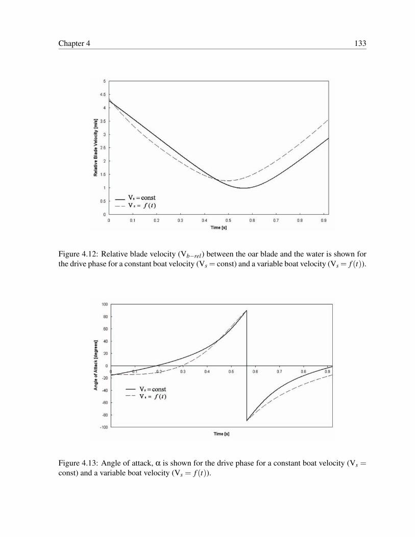
Chapter 4 133

Figure 4.12: Relative blade velocity (Vb−rel) between the oar blade and the water is shown forthe drive phase for a constant boat velocity (Vs = const) and a variable boat velocity (Vs = f (t)).

Figure 4.13: Angle of attack, α is shown for the drive phase for a constant boat velocity (Vs =const) and a variable boat velocity (Vs = f (t)).

Chapter 4 134

Figure 4.14: Temporal evolution of the hydrodynamic lift coefficient acting on the flat rectan-gular oar blade.

4.3.1 Flat rectangular oar

First the performance of the different turbulence models was investigated. Figures 4.14 and 4.15

compare the temporal evolution of the lift and drag coefficients from the CFD simulations using

the different turbulence models for the duration of one stroke (catch to finish). The flow time

was taken from 0 s, where t = 0 is at blade insertion (catch) and t = 0.92 was at blade removal

(finish). It can be seen that the k− ε variants (the realizable and RNG models) and the SST

k−ω model show almost identical values for both lift and drag coefficient during the course of

a stroke. However, the standard k−ε model shows some variation from the other models, which

would indicate that this model was less able to simulate the flow around the oar blade especially

at angles of attack where the flow was separated. This is consistent with what is suggested in

the literature [67, 88]. Of the other models, they all performed similarly and so SST k−ω was

selected to be consistent with the static simulations of Chapter 3. This turbulence model was

used for the remainder of the simulations and with the Big Blade oar design.

Comparison was made between the angular evolution of hydrodynamic force coefficients us-

Chapter 4 135

Figure 4.15: Temporal evolution of the hydrodynamic drag coefficient acting on the flat rectan-gular oar blade.

ing dynamic simulation and the equivalent quasi–static results. That is to say the lift and drag

coefficients at discrete angles of attack were compared with a continuous sample (taken every

1×10−3 s) of lift and drag coefficients obtained from the dynamic simulation. It was found in

Chapter 3 that it was important to use full scale blades, so that the quasi–static results which

were used are those from a full size flat rectangular oar, and for both the static and dynamic

situations the SST k−ω model was used.

In Figures 4.16 and 4.17 the lift and drag coefficients of the full size flat rectangular oar blade

held at stationary angles of attack to the oncoming flow are compared to a blade moving in a

continuous dynamic path through the same range of angles. First considering the lift coefficient

in Figure 4.16 it can be seen that the quasi–static lift forces generated by a static blade are,

in general, lower than those obtained when the blade is moving. This is especially true at the

beginning and end of the stroke, where α approaches 20 and 160 respectively. Here there was

a 56% and 72% difference between the static and dynamic values at these angles. At the other

angles there was a 45%–50% increase in the lift coefficient in the dynamic case. The absolute

Chapter 4 136

Figure 4.16: Angular evolution of the hydrodynamic lift coefficient acting on the flat rectangularoar blade.

Figure 4.17: Angular evolution of the hydrodynamic drag coefficient acting on the flat rectan-gular oar blade.

Chapter 4 137

Table 4.3: Absolute differences between the lift and drag coefficients generated by a quasi–staticand by a moving flat rectangular oar blade.

Angle (degrees) Absolute difference in CL Absolute difference in CD

20 0.99 0.3645 0.53 0.3370 0.46 0.9890 0.00 1.24

115 0.73 1.52135 1.19 1.19160 1.83 0.81

differences for each of the static angles tested are summarised in Table 4.3.

The drag coefficient, in Figure 4.17 also displays a reduction when the blade is static. Again

a similar pattern is seen as with the lift coefficient with the greatest percentage difference in

the static and dynamic values being seen early and late in the stroke. At 20 there was a 50%

difference and at 160 there was a 71% increase in drag coefficient from static to moving blade.

At the other angles the variation is between 35%–45%. Recalling from Chapter 3 that these

angles (20 and 160) were also the ones that showed the greatest discrepancy from the exper-

imental results. This again may indicate the deficiency of the numerical model to capture the

flow conditions at these angles.

As the bounded vortices, which theory suggest are produced [132], influence the forces which

develop around the blade, the development of the vorticity was plotted, which is a measure of

the angular rate of rotation of vortices. Figures 4.18(a–d) chart the vorticity in the flow field

around the flat rectangular oar blade where bright colours indicate higher levels of vorticity than

the cool colours. The upper limit of the contours was set at 200 s−1 so that the very high vortic-

ity present in the boundary layer close to the blade did not detract from the vorticity elsewhere.

At the catch (Figure 4.18a) it can be seen that a leading edge vortex has been formed and is

attached to the blade, it is during this part of the stroke that lift is the dominant force. As the

angle of attack increases in Figure 4.18b this vortex is subsequently shed and drag should begin

Chapter 4 138

to increase. The bright colour of these vortices indicate that they are fast moving. The blade

angle increases further past 90 in Figure 4.18c where a second fast moving vortex is formed at

the other edge (which is now the leading edge as the orientation of the blade has changed) and

lift is again being produced, but in the opposite sense. This vortex is still attached to the edge of

the blade in Figure 4.18d at finish, perhaps explaining why the lift is still quite large towards the

end of the stroke as was indicated in the numerical results in Figure 4.16. These results are in

agreement with the theoretical predictions of Young [132] shown in Figure 4.2, which indicates

a similar pattern of vortex formation and shedding.

It was discussed in Chapter 3 that it may be of benefit to harness such methods as DES or LES

which afford a much greater level of accuracy than RANS modelling. These techniques are

especially apt at simulating highly transient flows where such features as vortex generation and

shedding are occurring, as is seen here with the oar blade in motion. This progression to include

a DES or LES may well prove to be a worthwhile extension of the current work.

Variable inlet Velocity

The inlet velocity was set to be Vs = f (t) as defined in Section 4.2.3. For the flat rectangular oar

the lift and drag coefficients for this inlet velocity are compared with the results for Vs =const

in Figures 4.19 and 4.20. It can be seen that by having a variable inlet velocity the lift coeffi-

cient was not greatly effected by the change, except at small values of α (either in the positive

or negative sense).

The effect on drag coefficient was more substantial, here by having a variable inlet the drag co-

efficient was increased during the first half of the stroke and then was reduced during the second

half. Looking at Figure 4.12 it can be seen that this coincided with when Vb−rel was behaving

in the inverse manner. This is due to the inverse relationship between the drag coefficient and

V2b−rel .

When these results are compared to the static results, the trend is as before, where the lift coeffi-

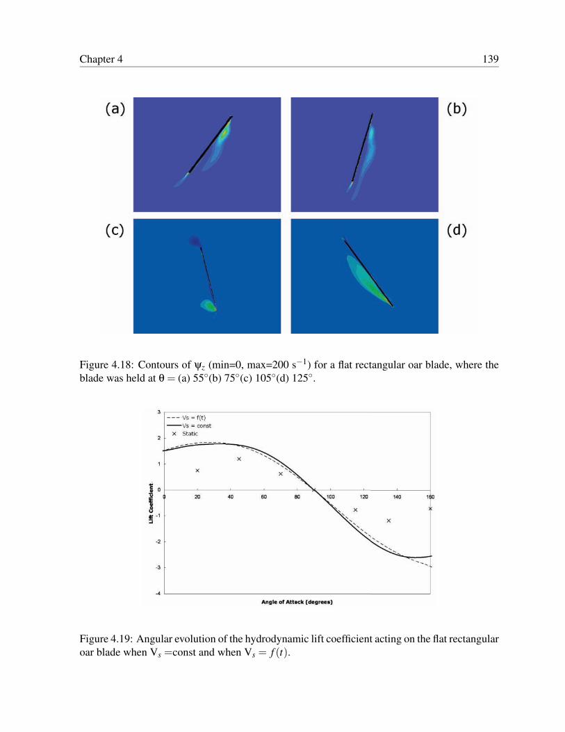
Chapter 4 139

Figure 4.18: Contours of ψz (min=0, max=200 s−1) for a flat rectangular oar blade, where theblade was held at θ = (a) 55(b) 75(c) 105(d) 125.

Figure 4.19: Angular evolution of the hydrodynamic lift coefficient acting on the flat rectangularoar blade when Vs =const and when Vs = f (t).

Chapter 4 140

Figure 4.20: Angular evolution of the hydrodynamic drag coefficient acting on the flat rectan-gular oar blade when Vs =const and when Vs = f (t).

cient is approximately the same as when Vs =const and the drag coefficient is now 35% greater

than the static values.

4.3.2 Big Blade

The lift and drag coefficients for a full size static Big Blade (obtained in Chapter 3) at discrete

angles of attack were compared with a continuous sample of lift and drag coefficients for the Big

Blade obtained from the dynamic simulation. For both the quasi–static and dynamic situations

the SST k−ω model was used. Figures 4.21 and 4.22 compare the lift and drag coefficients

of the Big Blade oar blade held at stationary angles of attack to the oncoming flow, to a blade

moving in a continuous dynamic path through the same range of angles.

Firstly, considering the lift coefficient in Figure 4.21 it can be seen that the lift forces generated

by a static blade are in most instances, like was seen with the flat rectangular oar, considerably

lower than those obtained when the blade is moving. If the two simulations are compared at

discrete angles in terms of their absolute differences (see Table 4.4) it can be observed that, in

Chapter 4 141

Figure 4.21: Angular evolution of the hydrodynamic lift coefficient acting on the Big Blade oar.Comparison is made between quasi–static and dynamic values.

general, the maximum unsteady lift is large when compared with the steady lift. This is consis-

tent with what has been found in previous studies [46, 125, 126]. Although, at α = 70 the static

value is 29% larger than the dynamic value, for the majority of the stroke dynamic lift is larger

than static. The maximum difference between the two values of lift coefficient occurs near the

start of the stroke when α = 20 where the dynamic value for lift coefficient is 72% larger than

the steady value. This is consistent with theory, which highlights the importance of considering

unsteadiness and start up vortices [128]. It has been discussed that with a quasi–static blade,

the vortex which is formed early on in the stroke needs time to gradually build up (known as

the Wagner effect [129]). When the blade was in motion it was not possible for a bound vortex

to develop in the same way as when it was stationary. By not considering the temporal changes

induced by the unsteady motion of the blade discrepancies arise.

In Figure 4.22 the drag coefficient variation for quasi–static and dynamic blades are compared.

Here, similarly, a reduction in drag coefficient was seen when the blade is static. Indeed the

reduction in drag coefficient when a quasi–static blade was considered was even more signif-

Chapter 4 142

Figure 4.22: Angular evolution of the hydrodynamic drag coefficient acting on the Big Bladeoar. Comparison is made between quasi–static and dynamic values.

Table 4.4: Absolute differences between the lift and drag coefficients generated by a quasi–staticand by a moving Big Blade oar.

Angle (degrees) Absolute difference in CL Absolute difference in CD

20 1.52 0.4145 0.95 0.7670 (- )0.91 1.5290 0.02 1.87

115 0.32 2.11135 1.23 1.54160 1.57 0.90

icant than with the lift coefficient. The maximum absolute difference in drag coefficient was

2.11 which equates to a 67% reduction from a moving blade and occurs at α = 115. Again

this is consistent with other similar work [46, 125, 126]. Further, it is evident that effects of

temporal changes inherent with the unsteady situation are more exaggerated with the Big Blade

than with the flat rectangular oar. This would suggest that the curvature of the blade is also

having an effect.

Chapter 4 143

Figure 4.23: Contours of vorticity (ωz) for Big Blade held at α = 45 (a) quasi- static simulation(b) dynamic simulation.

For both the lift and drag coefficients there was a significant discrepancy between quasi–static

and dynamic blades at the beginning of the stroke, close to the catch angle. This would sug-

gest that at catch the temporal changes are more apparent, perhaps highlighting the effect of

the difference in the way in which the start up vortices develop in the quasi–static and dynamic

situations. In Figure 4.23 the vorticity was compared at a blade angle of 45 for the quasi–static

and dynamic simulations. What is immediately apparent is that at α = 45 the blade angle (θ)

for the static and dynamic blades’ are different, this means that the relative velocity seen by

the quasi–static and dynamic blades is different, with the result that the vortices are formed on

different sides of the blade. However, if just the vortices are considered, independent of which

side of the blade they are on, in the dynamic simulation it can be seen in Figure 4.23b that a

bound vortex has formed and is still attached to the surface of the blade. This is indicative of lift

being produced. Whereas, at the same angle for the static simulation in Figure 4.23a the vortex

does not encapsulate the blade and has separated away from the surface, so the lift should be,

and is, much lower for the static blade in Figure 4.23a.

Variable inlet velocity

Similarly to the flat rectangular oar, the inlet was modified to vary with respect to time. Again

the lift and drag coefficients were monitored and compared to the constant velocity inlet and

Chapter 4 144

Figure 4.24: Angular evolution of the hydrodynamic lift coefficient acting on the Big Blade oarblade when Vs =const and when Vs = f (t). Static values are also given.

static simulations in Figures 4.24 and 4.25. It can be seen that, as for the flat rectangular oar

blade, the variable inlet (Vs = f (t)) produces greater values of lift coefficient over the constant

inlet (Vs =const) in the first half of the stroke. Whilst in the second half of the stroke the effect

is largely reversed. A similar pattern is evident for the drag coefficient in Figure 4.25. Again

the reason for this can be related back to Figure 4.12 which compared the relative blade velocity

(Vb−rel) during the drive phase for Vs = f (t) and Vs =const. It was shown that during the first

part of the stroke Vb−rel was higher for Vs =const and during the second half of the stroke it

Vb−rel was higher for Vs = f (t). As lift and drag coefficient are inversely proportional to the

square of Vb−rel (Equations 4.9 and 4.10) this provides an explanation for why the coefficients

are varying in this way.

Chapter 4 145

Figure 4.25: Angular evolution of the hydrodynamic drag coefficient acting on the Big Bladeoar blade when Vs =const and when Vs = f (t). Static values are also given.

4.4 Summary

The quasi–static analysis of the oar blades achieved in Chapter 3 was an important step forward

in the study of the mechanisms that govern oar blade propulsion. However, since it did not take

into account the fluid dynamic effects of the unsteady and rotational aspects of the blade, the

mechanism of the lift and drag forces needed to be reconsidered.

The lift coefficients were found to be as much as 72% greater for both the flat rectangular oar

blade and the Big Blade, while the drag coefficients were as much as 50% and 67% greater

for the flat rectangular oar and Big Blade respectively, when the blade was in motion. This

was in agreement (although the magnitude of the difference was somewhat larger) with similar

work carried out on swimmers’ hands [33, 124] , ellipsoids [126] and flat rectangular plates of

similar areas as oar blades [46] which also found that the propulsive forces were lower in the

quasi–static data than when in motion.

It has also been shown that the differences in the quasi–static and unsteady values could be

Chapter 4 146

attributed in part to the start up vortices which are present in the unsteady situation but not with

the stationary blades, as shown in Figure 4.23.

Having a variable inlet velocity when the moving blade is considered also affects the magnitude

of the lift and drag coefficients. This was due to the relative blade velocity being different for

a constant inlet and variable inlet. As the relative blade velocity is inversely proportional to the

lift and drag coefficients, it was unsurprising that they were affected. When compared to the

static values, the variable inlet showed an increase in the lift and drag coefficients, where the

maximum increase was approximately 35%.

It was shown that the local flow around the blade was very much influenced by both the rotation

of the blade around the oarlock, as well as the translational motion. Thus, the conclusion can

be made that it may not be appropriate to view an oar as a separate propelling surface for

which the force–producing characteristics can be determined in isolation in a water flume. The

current CFD models should not be viewed as an exact prediction of blade performance, more

so an indicator of the fluid dynamic forces acting on the blade. This understanding of how

a blade behaves when stationary or in motion can be utilised through a greater understanding

of the physics within a given design and also through allowing relative, rather than absolute,

comparison between designs.

Chapter 5

Simulations using Mathematical Model of

Rowing

5.1 Introduction

In Chapters 3 and 4 the fluid dynamic characteristics of oar blades were considered, and the

use of CFD techniques for modelling the fluid flow around them was validated for both static

blades and oar blades in motion. The aim of this chapter is to provide a means of linking the

work of Chapters 3 and 4, concerning just the oar blades, to the complete system of rowing

which includes the rower and boat, as well as the oar blades.

In Chapter 1 a number of mathematical models of rowing were introduced and it was shown

that it is possible to represent each component of the rowing system mathematically. Through

incorporating the propulsive properties of the oar blades into a larger mathematical model of

rowing, it should be possible to determine the performance of the rowing boat. Therefore,

propulsive force data obtained from the oar blades in Chapters 3 and 4 were integrated into a

mathematical model of rowing. In doing so it was possible to make an assessment not only of

the performance of the oar blades, but also to determine whether choosing a dynamic or a static

147

Chapter 5 148

approach to modelling the flow around the oar blades influenced the overall prediction of boat

performance significantly.

5.2 Model derivation

The mathematical model that was used for the simulations was based on the work of Caplan &

Gardner [57].

From Newton’s second law of motion:

∑F = ma (5.1)

where, F is the resultant of forces acting on the boat, arising from the forces applied by the

rowers at the oar blade, from the motion of the crew relative to the boat, and from the sources of

hydrodynamic and aerodynamic resistances acting on the boat. ‘m’ is the total crew–boat mass

and ‘a’ is the acceleration of the boat. Equation 5.1 can therefore be expanded:

P−Dr = msdvs

dt+mc

dvc

dt+

dvs

dt

(5.2)

where, P is the propulsive force produced by the crew and Dr is the total resistance force, ms

is the mass of the boat, oars and coxswain and mc is the combined mass of the crew, vs is the

absolute velocity of the boat and vc is the velocity of the crew relative to the boat. The resistive

term Dr, is comprised of hydrodynamic drag and aerodynamic drag, where the hydrodynamic

drag is obtained empirically from experimental work by Wellicome [61] and the aerodynamic

drag from experimental work by Hoerner [62] so that:

Dr = 13.05v2s −11.22vs +24.93+n(0.348v2

s ) (5.3)

Chapter 5 149

where, n is the number of rowers [58].

The motion of the rowers can be considered as masses moving with half a period of simple

harmonic motion [55, 60], where the motion of the crew centre of mass during the drive phase,

x1 is:

x1 =−ac cosptτ1

(5.4)

where, ac is the amplitude of the rowers movements fore and aft in the boat, τ1 is the duration

of the drive phase, and 0≤ t ≤ τ1. During the recovery phase this relationship is reversed, such

that the centre of mass position of the crew, x2 is:

x2 = ac cosptτ2

(5.5)

where, τ2 is the duration of the recovery phase and τ1 ≤ t ≤ τ1 +τ2. The centre of mass position

of the crew throughout the stroke is then differentiated to give the velocity of the crew centre of

mass during the drive phase of the stroke as:

Vc = x1 (5.6)

and

Vc = x2 (5.7)

during the recovery phase.

The propulsive force, P was defined by Pope [4] as the component of the blade force which

acts in line with the longitudinal axis of the boat, against the resistive forces, to propel the boat

forward. Now, from Equations 4.2 – 4.10 the resultant oar blade fluid force can be determined

as:

FB =q

F2L +F2

D (5.8)

Chapter 5 150

Figure 5.1: Forces acting normal and tangential relative to the oar blade chord line and directionof relative fluid flow (modified from Caplan & Gardner [57]).

Considering Figure 5.1, which defines the angles b = (90−α)+ α1 and α1 = cos−1(

FLFD

), so

that the normal and tangential components of this blade force acting are given by:

FBn = FB sinb (5.9)

and

FBt = FB cosb (5.10)

From Figure 5.1 it is seen that P can be obtained by resolving the normal and tangential forces,

so that:

P = FBn sinθ+FBt cosθ (5.11)

The only forces therefore acting externally on the rower–boat–oar system are the drag forces

acting on the shell, and the fluid force acting on the oar blade. It is the difference between these

Chapter 5 151

two forces, along with the forces generated by the acceleration of the crew within the boat,

which act to accelerate the boat forwards. By rearranging Equation 5.2 this acceleration can

therefore be defined as:

dvsdt

=

(P−Dr−mc

dvcdt

)(mc +ms)

(5.12)

where, P, Dr and dvcdt have been defined earlier.

5.3 Methodology

The mathematical model that was described in the preceding section was built in Simulink

(Matlab, Mathworks, USA) and was solved using the in–built Runge–Kutta variable rate solver

with a time step of 5× 10−3 s. The inputs into the model were kept constant for the purposes

of this investigation and are summarised in Table 5.1. In addition to these values, the shell drag

Table 5.1: Inputs into Simulink model of rowing.VariableStroke rate 30Total time (s) 2.00Drive time (s) 0.91Recovery time (s) 1.08Number of rowers 8Rower height (m) 0.92Rower mass (kg) 92.5Combined rower mass (kg) 740Combined boat & coxswain mass (kg) 146Outboard oar length (m) 2.365Water temperature (C) 16

coefficient was taken from Wellicome [61] and the air drag was assumed to be equal to that of a

seated man [59, 62], multiplied by the number of rowers in the boat [58]. The values which were

varied were the area of the oar blades and their force coefficients, which were specified from the

data obtained in Chapters 3 and 4 and from experimental work by Caplan & Gardner [22]. The

Chapter 5 152

flat rectangular oar, Big Blade and Macon oar blade designs were used in the quasi–static case

(Section 5.4) and a flat rectangular oar and the Big Blade in the dynamic case (Section 5.5). The

blade area of these full size blades was 0.124 m2 for both the flat rectangular oar and the Big

Blade and 0.107 m2 for the Macon oar (NB there were eight blades, as there were eight sweep

rowers).

5.4 Quasi–static input

In rowing the blade will move continuously through a path from catch to finish, however, with

the quasi–static model only a discrete number of angles were sampled; 0, 20, 45, 70, 90,

115, 135, 160, 180. In order for the mathematical model to create an accurate picture of

what is happening at the angles in between those sampled a piecewise cubic spline interpola-

tion was carried out to give a continuous reading of the values of lift and drag coefficient from

0−180.

The quasi–static results for oar blade lift and drag coefficients obtained for the flat rectangular

oar, Big Blade and Macon blade were input into the Simulink rowing model, allowing a com-

parison of the Caplan & Gardner [22] experiments and CFD predicted boat velocities. This

provided further validation of the CFD predictions for lift and drag coefficient which was based

on performance. The values from the CFD work that were used were those obtained from the

SST k−ω model, as this turbulence model consistently produced the most accurate predictions

of lift and drag coefficients, as was described in Chapter 3.

Once the CFD predictions for the boat velocity were compared against the Caplan & Gard-

ner [22] experimental values, analysis of the performance of the different blade designs was

made using only the CFD predicted values of lift and drag coefficient as an input.

Chapter 5 153

Figure 5.2: Variation in boat velocity during a rowing stroke using a flat rectangular oar blade.Comparison of Caplan & Gardner [22] experiments and CFD predictions of lift and drag coef-ficient as an input to rowing model.

5.4.1 Validation using rowing model

First considering the flat rectangular oar, the values of lift and drag coefficient obtained in Chap-

ter 3 were input into the Simulink rowing model, along with other variables defined in Table 5.1.

One stroke was isolated over many that will occur during the race, a stroke was selected that

occurred 90 s into the race, when the boat had reached a steady state velocity, after accelerating

during the first 500 m of a 2000 m race (Figure 5.2). The velocity profile seen in this figure has

been discussed in detail in Chapter 1.

Comparing the two simulations it can be seen that they show good agreement to one another,

with very similar changes in boat velocity over the course of the stroke. There is a maximum

over–estimation of the boat velocity of around 4% occurring at 0.35 s. The reason for this can

be traced to the errors seen in the predictions of lift and drag coefficients from the Caplan &

Chapter 5 154

Figure 5.3: Variation in boat velocity during a rowing stroke using a Big Blade oar. Comparisonof Caplan & Gardner [22] experiments and CFD predictions of lift and drag coefficient as aninput to rowing model.

Gardner [22] experimental and CFD work and equates to those angles where most error was

seen; namely 20 and 160.

In Figure 5.3 the boat velocity for a Big Blade is plotted, where again CFD and Caplan & Gard-

ner [22] experimental predictions for boat velocity are compared. The agreement between the

Caplan & Gardner [22] experimental and CFD performance predictions was very good, with

only a very small over–estimation of boat velocity when using the CFD results. A maximum

error of around 0.5% was found at 0.38 s. The errors were due to the lift and drag coefficients

also displaying some differences between the Caplan & Gardner [22] experiments and CFD

values. However, it can be seen that the effect this had on the overall prediction of performance

was very small.

The final blade that was investigated was the Macon blade which had a smaller projected blade

Chapter 5 155

Figure 5.4: Variation in boat velocity during a rowing stroke using a Macon oar blade. Com-parison of Caplan & Gardner [22] experiments and CFD predictions of lift and drag coefficientas an input to rowing model.

area than the other two oars, of 0.107 m2. Similarly, the Macon blade showed excellent agree-

ment between the experimental and CFD simulations throughout the drive phase of the stroke,

as shown in Figure 5.4. The greatest inaccuracy was an under–estimation when using the CFD

values by around 0.5%. Again any errors that were incurred during the CFD prediction of the

lift and drag coefficients did not translate into large errors in the prediction of boat velocity

during the rowing stroke.

Given these results and the confidence they afforded, it was then possible to use just the CFD

values of lift and drag coefficient as an input to the Simulink rowing model, to assess the perfor-

mance of the oar blades. Therefore, all subsequent simulations in this section, using the rowing

model, used the CFD values of lift and drag coefficient as an input.

Chapter 5 156

Figure 5.5: Mean boat velocity, using the CFD simulations as an input to rowing model, for aflat rectangular oar, Big Blade and Macon (actual area and Big Blade area) oar blades.

5.4.2 Oar blade performance

In order to gain an understanding of the effect of blade design on the performance of the boat,

it is worthwhile examining the mean boat velocity during the stroke. In Figure 5.5 it can be

seen that the predicted mean boat velocity is lowest for the Macon blade and highest for the Big

Blade, with the flat rectangular oar having a similar predicted mean velocity to the Big Blade.

As the boat is known to accelerate during the first 500 m of a 2000 m race [58], it might be more

appropriate to calculate the time travelled at mean boat velocity for the remaining 1500 m of a

typical race. Table 5.2 shows the time taken to travel this distance using each oar blade, along

with the difference in distance travelled using the Big Blade as the reference point.

What is useful to highlight at this point is the real advantage of this kind of analysis. Perfor-

mance has been measured here in terms of race time for each blade. However, we know that

Chapter 5 157

there are errors in the techniques that were used, that are of the order of seconds, this means

that these times are never going to be predictive of actual race times. It is therefore not the aim

to accurately predict these race times, but instead to allow comparison of blade designs relative

to one another. This enables trends between blade designs to be analysed, which is of much

greater use to rowing research community.

A substantial difference in rowing performance is seen between the Macon and the Big Blade

oars, with a smaller difference being seen between the Big Blade and the flat rectangular oar. As

Table 5.2: Comparison of oar blade designs showing the difference in time to complete 1500 mand the relative distance between the boats.

Blade Velocity (ms−1) Time for 1500 m (s) Distance over Big Blade (m)Macon 5.314 282.0 -42.28Flat rectangular oar 5.445 275.6 -6.32Big Blade 5.468 274.5 0.00

all the other variables were kept constant, the performance was a function of the blade area and

the force coefficients produced by the blade. Since the Macon blade has a significantly smaller

projected area than the Big Blade, the affect of this variable can be nullified by increasing the

projected area of the Macon blade to that of the Big Blade in the Simulink rowing model and

plotting it too () in Figure 5.5. It can be seen that the mean boat velocity is still lower for the

Macon. Therefore, it may be concluded that it was the forces that were being produced by the

blades, and not the blade area, that produced a reduction in the boat velocity with the Macon

blade. Although the force coefficients of the Big Blade and Macon blades were presented in

Figures 3.19, 3.20 and 3.21, they cannot be adjusted for an increase in blade projected area.

However, the lift and drag forces produced by the blades can be isolated as an output from the

Simulink rowing model and are plotted together for the Big Blade and Macon oars (of the same

projected area) over one stroke in Figures 5.6 and 5.7. From these figures the temporal devel-

opment of the forces over the course of a stroke can be chartered for the two blades. The forces

that are generated depends on the blade, the oar shaft angular velocity and the boat velocity

Chapter 5 158

Figure 5.6: Lift forces during the drive phase for the Big Blade and Macon oar blades, whereboth blades have the same projected area.

Chapter 5 159

Figure 5.7: Drag forces during the drive phase for the Big Blade and Macon oar blades, whereboth blades have the same projected area.

Chapter 5 160

Figure 5.8: Variation of angle of attack (degrees) during the drive phase of the stroke for theBig Blade and the Macon blade.

throughout the stroke. The angle of attack does not change linearly instead it varies as is shown

in Figure 5.8. What is evident for both blades is that early on in the stroke, when the angle

of attack is small < 20 the lift force increases to its first maximum rapidly, while drag force

increases more gradually until it reaches a peak at t≈ 0.32 s. Lift will reach its second peak

shortly after this at t≈ 0.36 s, however given the non- linearity of the angle of attack the blade

will have quickly changed the angle it makes with the free stream in this short time. As the

stroke progresses lift reduces quickly to a minimum at t≈ 0.58 s, while drag force peaks again

at the same time, this is when the blade is at 90. As the drive continues, the lift force will again

peak at t≈ 0.65 s (115) before finally reducing to zero at the end of the drive. The drag force

gradually reduces to zero as it approaches the end of the drive phase as well.

The lift forces produced by the Macon blade (see Figure 5.6) were significantly lower than those

produced by the Big Blade when t≈ 0.35 s and again when t≈ 0.65 s. The drag forces (see Fig-

ure 5.7) were significantly lower for the Big Blade when t≈ 0.35 s and t≈ 0.60 s. By plotting

Chapter 5 161

Figure 5.9: Contours of pressure coefficient at α = 20 for (a) Big Blade (b) Macon oar. Wherecool colours represent negative Cp and warm colours positive Cp.

the change in angle of attack during the drive phase of the stroke (Figure 5.8) it was further

possible to determine what angle of attack these differing forces were actually being produced

at. Although it is evident from Figure 5.8 that the angle of attack of the blade is between 0 and

90 for the majority of the stroke, the greatest difference in lift and drag force occurs early in the

stroke when α≈ 26 and then towards the end of the drive when α≈ 166 (which is equivalent

to −14 in Figure 5.8).

To understand why there are such differences in the forces produced it is useful to look at the

pressure distributions around the blades. In Figures 5.9 and 5.10 contours of pressure coeffi-

cient (Cp) for the Big Blade and Macon blades are plotted at α = 20 and α = 160 respectively

(of the static angles investigated these were the closest to the angles of interest). These plots

were produced through postprocessing of the solution in Fluent, where the warm colours show a

positive pressure coefficient, and the cool colours a negative pressure coefficient. The pressure

coefficient is negative on the upper surface, since the actual pressure is less than the ambient

pressure. Below the blade, on the facing surface, there are positive pressure coefficients, and

adding the forces on both sides on the blade leads to a net lift. Comparing the Macon and Big

Blade oars indicates that there is a difference in how the pressure is distributed on either side of

the blade. These discrepancies will result in different lift profiles at the angles presented, and

serve to reinforce the findings from the numerical results presented earlier.

Chapter 5 162

Figure 5.10: Contours of pressure coefficient at α = 160 for (a) Big Blade (b) Macon oar.Where cool colours represent negative Cp and warm colours positive Cp.

5.4.3 Comparing full size and quarter scale predictions

In Chapter 3 it was identified that it was important to model the blade as a full size blade, rather

than a quarter scale model. Therefore, the validity of this assumption was also investigated

by using the Simulink rowing model to examine relative boat performance. The lift and drag

coefficients for the flat rectangular, Big Blade and Macon oars were all input, as before, into the

model, and the boat velocities compared with their quarter scale counterparts (Figures 5.11, 5.12

and 5.13). It can be seen that for all three blades the full size blades produced a lower boat

velocity during a given stroke, than the quarter scale blades. This is a direct consequence of

the lift and drag coefficients being lower for the full size than the quarter scale blades. If the

mean boat velocities are plotted and compared between quarter and full scale (Figure 5.14) it

can be seen that although a similar trend between designs is clearly evident there is a lower

mean boat velocity when using full size blade coefficients as an input. However, given that this

boat velocity was lower by a seemingly consistent amount it may well be possible to use this as

a scaling factor, if only quarter scale blade data are available.

Chapter 5 163

Figure 5.11: Variation in boat velocity during a rowing stroke when using a flat rectangular oar.Comparison of quarter scale and full size blades.

Figure 5.12: Variation in boat velocity during a rowing stroke when using a Big Blade oar.Comparison of quarter scale and full size blades.

Chapter 5 164

Figure 5.13: Variation in boat velocity during a rowing stroke when using a Macon oar. Com-parison of quarter scale and full size blades.

Figure 5.14: Mean boat velocity for flat rectangular oar, Big Blade and Macon (actual area andBig Blade area) blades. Comparison of quarter scale and full size blades.

Chapter 5 165

5.5 Dynamic input

The dynamic results for oar blade lift and drag coefficients obtained for the flat rectangular oar

and Big Blade oars in Chapter 4 were also input into the Simulink rowing model. As with the

static blades all the other variables in Table 5.1 were kept constant, as was the projected blade

area.

Firstly, predictions of boat performance from the rowing model when the dynamic values were

used as an input were compared with measured on–water data for boat velocity obtained by

Kleshnev [11]. This provided a means of validating the dynamic model against real world

rowing data. Secondly, the dynamic and static model predictions were compared, allowing

insight as to how this difference in modelling technique influences the boat velocity.

5.5.1 Comparison against on water data

In Figure 5.15 the measured boat velocity of on–water rowing data obtained by Kleshnev [11] is

presented. These measured data are compared with the prediction of boat velocity by the rowing

model, using the dynamic CFD values as an input for lift and drag coefficients. Finally these

were compared with experimental values from Caplan & Gardner [22]. In all three situations

a men’s eight, rowing with the Big Blade oar was investigated. It can be seen that a good

approximation for boat velocity during the stroke was obtained when using the dynamic CFD

values were used. During the middle section of the drive phase of the stroke (0.3 < t < 0.7) there

was a better approximation than was found with the experimental values, however, towards the

end of the drive and during the majority of the recovery (0.7 < t < 1.5) the CFD simulation

over–predicts boat velocity. In Figure 5.16 the mean boat velocity obtained from the rowing

model, when the dynamic CFD results were used as an input, were compared with the average

of the on–water data from Kleshnev [11]. The modelled mean boat velocity is also presented

when the experimental values of Caplan & Gardner [22] were used. It can be seen that a good

Chapter 5 166

Figure 5.15: On–water measured boat velocity from Kleshnev [11] and modelled boat velocityusing experimental results from Caplan & Gardner [22] and dynamic CFD results as an input.Results are shown for one complete stroke.

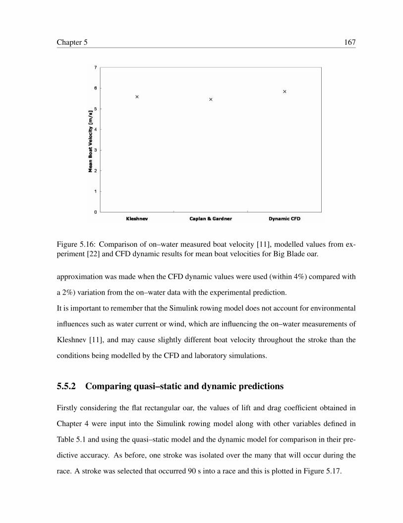
Chapter 5 167

Figure 5.16: Comparison of on–water measured boat velocity [11], modelled values from ex-periment [22] and CFD dynamic results for mean boat velocities for Big Blade oar.

approximation was made when the CFD dynamic values were used (within 4%) compared with

a 2%) variation from the on–water data with the experimental prediction.

It is important to remember that the Simulink rowing model does not account for environmental

influences such as water current or wind, which are influencing the on–water measurements of

Kleshnev [11], and may cause slightly different boat velocity throughout the stroke than the

conditions being modelled by the CFD and laboratory simulations.

5.5.2 Comparing quasi–static and dynamic predictions

Firstly considering the flat rectangular oar, the values of lift and drag coefficient obtained in

Chapter 4 were input into the Simulink rowing model along with other variables defined in

Table 5.1 and using the quasi–static model and the dynamic model for comparison in their pre-

dictive accuracy. As before, one stroke was isolated over the many that will occur during the

race. A stroke was selected that occurred 90 s into a race and this is plotted in Figure 5.17.

Chapter 5 168

Figure 5.17: Boat velocity predictions for flat rectangular oar during one stroke when static anddynamic CFD results are used as an input.

Comparing the two simulations it can be seen that they show a good correlation to one another,

showing similar changes in boat velocity over the course of the stroke. However, when the dy-

namic CFD values were used as an input to the model the boat velocity was consistently greater

throughout the duration of one stroke. In order to quantify this the mean boat velocities can be

compared. When static CFD values were used as an input the mean boat velocity obtained was

5.41 ms−1 and when dynamic values were used the mean boat velocity rose to 5.69 ms−1; this

is a 5.1% increase. It was found in Chapter 4 that significantly different values for lift and drag

coefficient during the stroke were obtained between dynamic (unsteady) and static approaches.

In Figure 5.18 the boat velocity over a stroke was compared for static and dynamic values of

lift and drag coefficients, when a Big Blade oar was used. It is clear that, as with the flat rect-

angular oar, the dynamic values indicate a higher boat velocity during the stroke, than when

static values are used. Again, if the mean boat velocities are compared they were 5.47 ms−1

and 5.84ms−1 for the static and dynamic inputs respectively. This equates to a 6.7% increase

for when dynamic values of lift and drag coefficient are used as an input into the model when

Chapter 5 169

Figure 5.18: Boat velocity predictions for Big Blade oar during one stroke when static anddynamic CFD results are used as an input.

using a Big Blade oar.

There was significant variation between the static and dynamic predictions of boat performance,

however, it was shown in Section 5.5.1 that when compared to on–water measured data for boat

velocity, both make feasible predictions.

5.6 Summary

This chapter has integrated the work of Chapters 3 and 4 where the force coefficients of a

number of different oar blades were input into a Simulink rowing model. When the quasi–

static values of lift and drag coefficient were used a very good approximation was made to the

experimental results of Caplan & Gardner [22] (within 4% for flat rectangular blade, 0.5% for

the Big Blade and 0.5% for the Macon blade). When full size and quarter scale values for

lift and drag coefficient were input into the model, it was found, for all three blades, that the

full size blades produced a lower boat velocity during a given stroke than their quarter scale

Chapter 5 170

counterparts.

Using the quasi–static results it was also possible to undertake some analysis on the effect of

blade design on performance. By comparing the forces produced by the blades it was clear

that the Big Blade was able to attain much higher lift forces that the Macon blade. Further

understanding was provided by plotting pressure coefficient contours around the blade which

showed discrepancies in the pressure differentials between the upper and lower surfaces of the

Big Blade and the Macon blade.

Using the data obtained from Chapter 4 it was further possible to produce predictions of boat

velocity using the force coefficients of a blade in motion as an input. It was shown that when

compared to on–water measured data for boat velocity obtained by Kleshnev [11], that a good

correlation was found. The mean boat velocity was within 4% of the on–water mean value,

whilst the predictions using the experimental values of Caplan & Gardner [22] were within 2%

of the on–water mean velocity.

It has been shown that it is possible to use CFD predictions of force coefficients of oar blades

to provide an accurate assessment of boat performance during the rowing stroke. Both quasi–

static and dynamic approaches to measuring these forces produced results which correlated

favourably with measured on–water data.

It is envisaged that rather than to use the CFD models to compare blades in terms of their

absolute performance, it will be utilised to allow their relative performance to each other to be

ascertained, as an aid design. It is clearly not possible to predict, to any sort of useful level,

how a blade would actually influence performance, once it is realised that races are won, and

lost, in fractions of seconds, while the magnitude of the errors in the model are of the order

of seconds. Combined with further CFD work which may be extended to include DES or LES

simulations of the flow around rowing oar blades, this highlights the great potential of using

CFD techniques as an aid to oar blade design.

Chapter 6

Conclusions and Future Work

The aims of the thesis were outlined in Chapter 1 and the primary objective, to use CFD to

investigate the fluid flow around rowing oar blades, was identified. Through an examination

of the existing research, it was determined that the analysis of the fluid flow around compe-

tition oar blades had received very little attention. Instead the majority of CFD studies had

focused on rectangular plates of the same projected area (or a scaling factor thereof) as an oar

blade [30, 31, 46]. Further, very limited work had been undertaken to establish a link between

any CFD studies on oar blades and rowing performance.

A CFD model has been validated against experimental data for the performance of four types

of oar blade using the blade force coefficients of lift and drag. It was found that the SST k−ω

turbulence model produced the best correlation with the data for all four oar blades and at all

angles of attack

It was expected that further accuracy could be obtained if the free surface interactions between

water and air at the top of the flume was also modelled. A VOF model of the free surface was

therefore also incorporated into the CFD model. It was found that although the actual physi-

cal representation of the free surface was indeed much like actual experimental conditions, the

numerical values of lift and drag coefficient were not significantly closer to the experimental

171

Chapter 6 172

values and, due to ventilation and blockage effects, the drag was under–predicted.

The CFD model was used to extend the current research to investigate full size oar blades of the

design used in competition. Previous experimental work had been constrained by the inability

to match dynamic similarity and it was found, through the use of CFD predictions, that it is nec-

essary to match dynamic similarity. Without it the lift and drag coefficients were significantly

larger than they should be at full size, this is in agreement with previous work undertaken on

flat rectangular plates [46].

Visualisations of the flow offered details such as velocity magnitude and pressure distributions

in the flow field around the blade, providing more insight into oar blade fluid dynamics than

physical experimentation alone had achieved.

The quasi–static analysis of the oar blades achieved in Chapter 3 was an important step for-

ward in the study of the mechanisms that govern oar blade propulsion. Although this kind of

analysis is an accepted technique, having been previously used to investigate the flow around

swimmers’ hands [33, 34, 35], kayak paddles [36] and oar blades [22, 23], it had fundamental

shortcomings. Since a quasi–static analysis, by its very nature, does not take account of the

fluid dynamic effects of the unsteady and rotational aspects of the blade, its effect was likely to

be considerable and needed to be determined for oar blades. Further, a dynamic simulation has

the distinct advantage that fewer repetitions need be undertaken to represent the rowing stroke,

than with a quasi–static analysis.

Through utilising dynamic modelling techniques it was found that lift coefficients were as much

as 72% greater when the blade was in motion, than when it was static, for both a flat rectangular

oar blade and a Big Blade. The drag coefficients were as much as 50% and 67% greater for a flat

rectangular oar and Big Blade respectively, when the blade was in motion. These differences

could be attributed in part to the start up vortices which are present in the unsteady situation but

not with the stationary blades. This was found to be in agreement with similar work carried out

on swimmers’ hands [33, 124], ellipsoids [126] and flat rectangular plates of similar areas as

Chapter 6 173

oar blades [46] which had also found the propulsive forces to be considerably lower.

It was shown that the local flow around the blade was very much influenced by both the rotation

of the blade around the oarlock, as well as the translational motion. It may not be appropriate to

view an oar as a separate propelling surface for which the force–producing characteristics can

be determined in isolation in a water flume.

In order to establish the influence that the oar blades were having on boat performance, predic-

tions of boat velocity were made using the force coefficients obtained in Chapters 3 and 4. The

CFD data obtained for the quasi–static and dynamic oar blades was coupled with a previously

validated mathematical model of rowing, and it was shown that it is possible to use these pre-

dictions of force coefficients of oar blades to provide an assessment of boat performance during

the rowing stroke. Both the static and dynamic predictions provided acceptable approximations

when compared to both the experimental results of Caplan & Gardner [22] and to on–water

measured data for boat velocity obtained by Kleshnev [11]. However, the experimental results

of Caplan & Gardner [22] were still marginally more accurate throughout the stroke.

In conclusion, CFD techniques have been shown to provide a valid and accurate simulation of

the fluid dynamics of oar blade propulsion. However, there is still scope for the CFD modelling

to be further improved by allowing for variable oar blade angular velocity, which is present in

rowing, but has not been incorporated into the present research. It is also recommended that

future work should continue to use a combination of CFD simulations and the mathematical

model of rowing to investigate and optimise other oar blade designs.

It was discussed in Chapter 3 that it may be of benefit to harness such methods as DES or LES

which afford a much greater level of accuracy than RANS modelling. These techniques are

especially apt at simulating highly transient flows where such features as vortex generation and

shedding are produced, as is seen with the oar blades. This progression to include a DES or

LES may well prove to be a worthwhile extension of the current work.

It is envisaged that rather than to use the CFD models to compare blades in terms of their abso-

lute performance, it will be utilised to determine their relative performance to one another as an

aid to future oar blade design.

174

List of References

[1] A. Dal Monte and A. Komor, “Rowing and sculling mechanics,” in Biomechanics ofSport, C. Vaughan, Ed. Florida: CRC Press Inc., 1989, pp. 53–120.

[2] World Rowing, url:http://80.83.47.230/nresults.fwx, cited 25.08.2009.

[3] D. Hartwanger and E. Bunt, “Modelling of scull drag at the orthogonal point of a rowingstroke.” University of Witwatersrand, South Africa, Msc, 1996.

[4] D. Pope, “On dynamics of men and boats and oars,” in Mechanics and Sport, J. Bleustein,Ed. New York: American Society of Mechanical Engineers, 1973, pp. 113–130.

[5] B. Munson, D. Young, and T. Okiishi, Fundamentals of uid mechanics (4th ed). NewYork: John Wiley and Sons Inc., 2002.

[6] B. Sayer, Rowing and sculling: the complete manual. London: St Edmundsbury PressLtd, 1996.

[7] V. Nolte, Rowing Faster. Illinois: Human Kinetics, 2004.

[8] E. Atkinson, “A rowing indicator,” Natural Science, vol. 8, p. 178, 1896.

[9] F. Alexander, “The theory of rowing,” University of Durham Philosophical Society, pp.160–179, 1926.

[10] E. Schneider and M. Hauser, “Biomechanical analysis of performance in rowing,” inBiomechanics VII-B, A. Morecki, K. Fidelus, K. Kedzior, and A. Wit, Eds. Baltimore:University Park Press, 1981, pp. 430–435.

[11] V. Kleshnev, “Propulsive efficiency of rowing,” in XVII International Symposium onBiomechnics in Sport, 1999, pp. 224–228.

[12] T. Martin and J. Bernfield, “Effect of stroke rate on the velocity of a rowing shell,”Medicine and Science in Sports and Exercise, vol. 12, pp. 250–256, 1980.

[13] Y. Aujouannet and A. Rounard, “Kinetic study of cyclic phases in rowing,” Journal ofHuman Movement Studies, vol. 46, pp. 303–318, 2004.

175

[14] F. Celentano, G. Cortili, P. Di Prampero, and P. Cerretelli, “Mechanical aspects of row-ing,” Journal of Applied Physiology, vol. 36, pp. 642–647, 1974.

[15] F. Coulloud, S. Manel, and A. Rounard, “3D kinematic relationships between blade andboat in rowing,” Journal of Human Movement Studies, vol. 40, pp. 83–100, 2001.

[16] V. Nolte, “Introduction to the biomechanics of rowing,” FISA Coach, vol. 2, pp. 1–6,1991.

[17] W. Gutschow, “Mechanik des getriebes ruderer/ruder,” Schiffstechnik, vol. 3, pp. 128–132, 1955.

[18] J. Wellicome, “Some hydrodynamic aspects of rowing,” in Rowing – a scientic ap-proach, A. Scott and J. Williams, Eds. New Jersey: A S Barnes and Co., 1967, pp.22–63.

[19] V. Kleshnev and I. Kleshnev, “Dependence of rowing performance and efficiency onmotor co-ordination of the main body segments,” Journal of Sports Sciences, vol. 16, pp.418–419, 1998.

[20] V. Nolte, Die effectivitat des ruderschlages. Berlin: Bartels and Wernitz, 1984.

[21] K. Affeld, K. Schichl, and A. Ziemann, “Assessment of rowing efficiency,” InternationalJournal of Sports Medicine, vol. 14(1), pp. 39–41, 1993.

[22] N. Caplan and T. Gardner, “A fluid dynamic investigation of the Big Blade and Maconoar blade designs,” Journal of Sports Sciences, vol. 25, pp. 643–650, 2007.

[23] N. Caplan and T. Gardner, “Optimisation of oar blade design for improved performancein rowing,” Journal of Sports Sciences, vol. 25, pp. 1471–1478, 2007.

[24] D. Dreissigacker and P. Dreissigacker, “Oars - theory and testing,” in Proceedings of theXXIX FISA Coaches Conference, Seville, Spain, 2000.

[25] N. Caplan, “A computer model to simulate the mechanics of rowing,” School of Sportand Exercise Sciences, University of Birmingham, UK, PhD Thesis, 2005.

[26] W. Bird, “The mechanics of sculling,” Chartered Mechanical Engineer, vol. 22, pp. 91–94, 1975.

[27] V. Zatsiorsky and N. Yakunin, “Mechanics and biomechanics of rowing: a review,” In-ternational Journal of Sports Biomechanics, vol. 7, pp. 229–281, 1991.

[28] A. Baudouin and D. Hawkins, “A biomechanical review of factors affecting rowing per-formance,” British Journal of Sports Medicine, vol. 36, pp. 396–402, 2002.

[29] S. Barre and J. Kobus, “New facilities for measurement of hydrodynamic loads on oarblades,” in Engineering of Sport, 1998, pp. 251–260.

176

[30] T. Kinoshita, M. Miyashita, H. Kobayashi, and T. Hino, “Rowing velocity predictionprogram which estimates hydrodynamic load acting on an oar blade,” in Bio-mechanismsof Animals in Swimming and Flying - ISABMEC, 2007.

[31] A. Leroyer, S. Barre, and J.-M. Kobus, “Experimental and numerical investigations ofthe flow around an oar blade,” Journal of Marine Science and Technology, vol. 13, pp.1–15, 2008.

[32] T. Pelham, L. Holt, K. Burton, A. Carter, and J. Peach, “The effect of oar design on scullboat dynamics,” in Proceedings of the XI International Symposium on Biomechanics inSports, 1993, pp. 201–204.

[33] H. Toussaint, C. Van den Berg, and W. Beek, “Pumped up propulsion during front crawlswimming,” Medicine and Science in Sports and Exercise, vol. 34, pp. 314–319, 2002.

[34] M. Berger, G. de Groot, and A. Hollander, “Hydrodynamic drag and lift forces on humanhand/arm models,” Journal of Biomechanics, vol. 28, pp. 125–133, 1995.

[35] B. Bixler and S. Riewald, “Analysis of a swimmers hand in steady flow conditions usingCFD,” Journal of Biomechanics, vol. 35, pp. 713–717, 2002.

[36] D. Sumner, E. Sprigings, J. Bugg, and J. Heseltine, “Fluid forces on kayak paddle bladesof different design,” Sports Engineering, vol. 6, pp. 11–20, 2003.

[37] S. Patankar, Numerical heat transfer and uid ow. New York: Hemisphere PublishingCoporation, 1980.

[38] C. Lueneburger, “A comparative analysis of Macon and ‘Big’ racing blades,” FISACoach, vol. 6, pp. 1–8, 1995.

[39] G. Cowles and N. Parolini, “CFD makes waves in the Americas Cup,” Fluent News, pp.20–23, 2002.

[40] R. Lukes, J. Hart, S. Chin, and S. Haake, “The role and validation of CFD applied tocycling,” in Fluent UGM, 2005, pp. 64–75.

[41] W. Keller, A. Savill, and W. Dawes, “Integrated CAD/CFD visualisation of a genericFormula 1 car front wheel flowfield,” in High-Performance Computing and Networking,vol. 1593, 1999, pp. 90–98.

[42] B. Bixler and M. Schloder, “Computational fluid dynamics: an analytical tool for the 21stcentury swimming scientist,” Journal of Swimming Research, vol. 11, pp. 4–22, 1996.

[43] A. Rouboa, A. Silva, L. Leal, J. Rocha, and F. Alves, “The effect of swimmer’shand/forearm acceleration on propulsive forces generation using computational fluid dy-namics,” Journal of Biomechanics, vol. 39, pp. 1239–1248, 2006.

177

[44] G. Lecrivain, A. Slaouti, C. Payton, and I. Kennedy, “Using reverse engineering and com-putational fluid dynamics to investigate a lower arm amputee swimmer’s performance,”Journal of Biomechanics, vol. 41, pp. 2855–2859, 2006.

[45] Speedo, url:http://www.speedo80.com/lzr-racer, cited 27.08.2009.

[46] A. Sliasas and S. Tullis, “Numerical modelling of rowing blade hydrodynamics,” SportsEngineering, vol. 12, pp. 31–40, 2009.

[47] E. Herberger, Rowing. Toronto: Sports Books Publisher, 1987.

[48] A. Duhida, A history of Oxford college rowing. url:http://www.atm.ox.ac.uk/rowing/history.html, cited 27.08.2009.

[49] P. Pinkerton, “The Big Blade goes big time,” Australian Rowing, vol. September, pp.10–11, 1992.

[50] R. Pomponi, “Innovations in oar technology: transition to a new dominant design,” Tech-nology Strategy, vol. December, 1994.

[51] Concept2, url:http://www.concept2.com, cited 19.04.2009.

[52] J. Dreher, Technology discussion: new blade shapes - part 1.url:http://www.durhamboat.com/blade1.php, cited 27.08.2009.

[53] V. Nolte, “Do you need hatchets to chop your water?” Am Rowing, vol. July/August, pp.23–26, 1993.

[54] V. Nolte, “Shorter oars are more effective,” Journal of Applied Biomechanics, vol. 25,pp. 1–8, 2009.

[55] M. Brearley and N. de Mestre, “Modelling the rowing stroke in racing shells,” in 3rdConference on Mathematics and Computers in Sport, Bond University, Queensland, Aus-tralia, 1996.

[56] D. Cabrera, A. Ruina, and V. Kleshnev, “A simple 1+ dimensional model of rowingmimics observed forces and motions,” Journal of Human Movement Science, vol. 25,no. 2, pp. 192–220, 2006.

[57] N. Caplan and T. Gardner, “A mathematical model of the oar blade – water interaction inrowing,” Journal of Sports Sciences, vol. 25, pp. 1–10, 2007.

[58] L. Lazauskas, “A performance prediction model for rowing races,” Department of Ap-plied Mathematics, University of Adelaide, Australia, Technical Report, 1997.

[59] A. Millward, “A study of the forces exerted by an oarsman and the effect on boat speed,”Journal of Sports Sciences, vol. 5, pp. 93–103, 1987.

178

[60] M. Brearley and N. de Mestre, “The effect of oar flexing on rowing performance,” in4th Conference on Mathematics and Computers in Sport, Bond University, Queensland,Australia, 1998.

[61] J. Wellicome, “Report on resistance experiments carried out on three racing shells,” Na-tional Physical Laboratory Ship Division, Technical Memorandum, 1967.

[62] S. Hoerner, Fluid dynamic drag. New Jersey: Hoerner, 1965.

[63] S. Hoerner and H. Borst, Fluid dynamic lift. New Jersey: Hoerner, 1985.

[64] C. Scragg and B. Nelson, “The design of an 8 oared rowing shell,” Marine TechnologySNAME News, vol. 30, pp. 84–99, 1993.

[65] J. Mitchell, “The wave resistance of a ship,” Philosophical Magazine, vol. 5, pp. 106–123, 1898.

[66] J. Anderson Jr, Computational uid dynamics – the basics with applications. New York:McGraw-Hill, 1995.

[67] J. Ferziger and M. Peric, Computational methods for uid dynamics. Berlin: Springer,2002.

[68] H. Versteeg and W. Malalalsekra, An introduction to computational uid dynamics. NewYork: Prentice Hall, 1996.

[69] D. Wilcox, Modelling for CFD. La Canada: DCW Industries Inc, 1998.

[70] O. C. Zienkiewicz, The nite element method. New York: McGraw-Hill, 1977.

[71] H. Morvan and D. M. Hargreaves, “Computational fluid dynamics summer school,” TheUniversity of Nottingham, Lecture Notes, 2007.

[72] V. Liseikin, Grid generation methods. Berlin: Springer, 1999.

[73] T. Stoesser, “Development and validation of a CFD code for turbulent open–channelflows,” University of Bristol, UK, PHD Thesis, 2001.

[74] R. Courant, K. Friedrichs, and H. Lewy, “Uber die partiellen Differenzengleichungen dermathematischen physik,” Mathematische Annalen, vol. 100, p. 3274, 1928.

[75] J. Blazek, Computational uid dynamics: principles and applications. Oxford: ElsevierScience Ltd, 2001.

[76] Flow 3D, url:http://www.flow3d.com/Cfd-101/turb.htm, cited 16.04.2009.

[77] A. Kolmorgorov, “The local structure of turbulence in incompressible viscous fluid forvery large Reynolds numbers,” Doklady Akademii Nauk SSSR, vol. 30, pp. 301–305,1941.

179

[78] J. Bardina, J. Ferziger, and W. Reynolds, “Improved subgrid models for large eddy sim-ulation,” AIAA Paper, pp. 80–1357, 1980.

[79] O. Reynolds, “On the dynamical theory of incompressible viscous fluids and the deter-mination of the criterion,” in Proceedings of the Royal Society of London, vol. 186, 1895,pp. 123–164.

[80] T. Gatski, M. Hussaini, and J. Lumley, Simulation and modelling of turbulent ows.New York: Oxford University Press, 1996.

[81] B. Launder and D. Spalding, “The numerical calculation of turbulent flows,” ComputerMethods in Applied Mechanics and Engineering, vol. 3(2), p. 269, 1974.

[82] S. Yuan, Foundation of uid mechanics. New Jersey: Prentice Hall, Inc., 1967.

[83] J. Boussinesq, “Theorie de l’ecoulement tourbillant (theories of swirling flow),” Mem.Presentes par Divers Savants a l'Acadademique Sciences, vol. 23, 1877.

[84] K. Shimada and T. Ishihara, “Application of a modified k− ε model to the predictionof aerodynamic characteristics of rectangular cross-section cylinders,” Journal of Fluidsand Structures, vol. 16, pp. 465–485, 2002.

[85] V. Yakhot, S. Orszag, S. Thangam, T. Gatski, and C. Speziale, “Development of tur-bulence models for shear flows by a double expansion technique,” Physics of Fluids A,vol. 4, pp. 1510–1520, 1992.

[86] G. Papageorgakis and D. Assanis, “Comparison of linear and nonlinear RNG-based k−ε

models for incompressible turbulent flows,” Numerical Heat Transfer Part B, vol. 35, pp.1–22, 1999.

[87] T.-H. Shih, W. Liou, A. Shabbir, Z. Yang, and J. Zhu, “A new k− ε eddy- viscositymodel for high reynolds number turbulent flows - model development and validation,”Computers and Fluids, vol. 24(3), pp. 227–238, 1995.

[88] Fluent, url:http://www.fluent.com, cited 12.04.2009.

[89] A. Beljaars, J. Walmsley, and P. Taylor, “A mixed spectral finite-difference model for neu-trally stratified boundary-layer flows over roughness changes and topography,” BoundaryLayer Meteorology, vol. 38, pp. 273–303, 1987.

[90] F. Mentor, “Two-equation eddy-viscosity turbulence models for engineering applica-tions,” American Institute of Aeronautics and Astronautics, vol. 32(8), pp. 1598–1605,1994.

[91] ANSYS, “Innovative turbulence modelling: shear stress transport SST model,” in ANSYSCFX http://www.ansys.com/assets/tech-briefs/PDF0072.pdf, 2004.

180

[92] P. Gauckler, “Etudes theoriques et pratiques sur l’ecoulement et le mouvement des eaux,”Comptes Rendues de l'Academie des Sciences, vol. 64, pp. 818–822, 1867.

[93] G. Tryggvason, B. Bunner, A. Esmaeeli, D. Juric, N. Al-Rawahi, W. Tauber, J. Han,S. Nas, and Y.-J. Jan, “A front-tracking method for the computations of multiphase flow,”Journal of Computational Physics, vol. 169, p. 708759, 2001.

[94] W.-T. Tsai and D. Yue, “Computation of nonlinear free-surface flows,” Annual Review ofFluid Mechanics, vol. 28, pp. 249–278, 1996.

[95] W. Shyy, H. Udaykumar, M. Rao, and R. Smith, Computational uid dynamics withmoving boundaries, Series in Computational and Physical Processes in Mechanics andThermal Sciences. Washington DC: Taylor and Francis, 1996.

[96] P. Zwart, G. Raithby, and M. Raw, “The integrated space-time finite volume method andits application to moving boundary problems.” Journal of Computational Physics, vol.154, pp. 497–519, 1999.

[97] J. The, G. Raithby, and G. Stubley, “Surface-adaptive finite-volume method for solvingfree surface flows,” Numerical Heat Transfer, Part B, vol. 26, pp. 367–380, 1994.

[98] S. Van der Pijl, “Free-boundary methods for multi-phase flows,” Delft University ofTechnology, Technical Report, 2004.

[99] F. Harlow and J. Welsh, “Numerical calculation of time-dependent viscous incompress-ible flow with a free surface,” Physics of Fluids, vol. 8, pp. 2182–2189, 1965.

[100] F. Harlow, A. Amsden, and J. Nix, “Relativistic fluid dynamics calculations with theparticle-in-cell technique,” Journal of Computational Physics, vol. 20, pp. 119–129,1976.

[101] C. Hirt and J. Shannon, “Free-surface stress conditions for incompressible–flow calcula-tions,” Journal of Computational Physics, vol. 2, pp. 403–411, 1968.

[102] C. Hirt and B. Nichols, “Volume of fluid (VOF) method for the dynamics of free bound-aries,” Journal of Computational Physics, vol. 39, pp. 201–225, 1981.

[103] D. L. Youngs, “Time-dependent multi-material flow with large fluid distortion,” Numer-ical Methods for Fluid Dynamics, 1982.

[104] S. Rhee and E. Koutsavdis, “Two-dimensional simulation of unsteady marine propul-sor blade flow using dynamic meshing techniques,” Computers and Fluids, vol. 34, pp.1152–1172, 2005.

[105] I. Demirdzic and M. Peric, “Space conservation law in finite volume calculations of fluidflow,” International Journal of Numerical Methods and Fluids, vol. 8, pp. 1037–1050,1988.

181

[106] D. Hargreaves, H. Morvan, and N. Wright, “Validation of the VOF method for free sur-face calculation: the broad crested weir,” Engineering Applications of ComputationalFluid Mechanics, vol. 1(2), pp. 136–146, 2007.

[107] K. Popper, The logic of scientic discovery. London: Taylor and Francis, 2003.

[108] I. Babuska and T. Oden, “Verification and validation in computational engineering andscience: basic concepts and applications,” Computer Methods in Applied Mechanics ofEngineering, vol. 193, pp. 4057–4066, 2004.

[109] J. E. Cermak and N. Isyumov, Wind tunnel studies of buildings and structures. USA:American Society of Civil Engineers, 1998.

[110] AIAA, “Guide for the verification and validation of computational fluid dynamic sim-ulations,” American Institute of Aeronautics and Astronautics, vol. AIAA-G-077-1998,1998.

[111] CIMdata, url:http://www.cimdata.com.html, cited 08.07.2009.

[112] B. Kader, “Temperature and concentration profiles in fully turbulent boundary layers,”International Journal of Heat and Mass Transfer, vol. 24(9), pp. 1541–4, 1981.

[113] R. I. Issa, “Solution of the implicitly discretized fluid flow equation by operator splitting,”Journal of Computational Physics, vol. 62, pp. 40–65, 1986.

[114] J. Doormaal and G. D. Raithby, “Enhancements of the simple method for predictingincompressible fluid flows,” Numerical Heat Transfer, vol. 7, pp. 147–163, 1984.

[115] E. Taylor, Dimensional analysis for engineers. Oxford: Oxford University Press, 1974.

[116] P. Davidson, Turbulence: an introduction for scientists and engineers. Oxford: OxfordUniversity Press, 2004.

[117] J. Mathieu and J. Scott, An introduction to turbulent ow (1st ed.). Cambridge: Cam-bridge University Press, 2000.

[118] S. Bradford, “Numerical simulation of surf zone dynamics,” Journal of Waterway, Port,Coastal and Ocean Engineering, vol. 126, pp. 1–13, 2000.

[119] T. Salaheldin, J. Imran, and M. Chaudhry, “Numerical modelling of three-dimensionalflow field around circular piers,” Journal of Hydraulic Engineering, vol. 130(2), pp. 91–100, 2004.

[120] M. Zhang and Y. Shen, “Three-dimensional simulation of meandering river based on 3-D k− ε RNG turbulence model,” Journal of Hydrodynamics, Series B, vol. 20(4), pp.448–455, 2008.

182

[121] C. Rhie and W. Chow, “A numerical study of the turbulent flow past an isolated airfoilwith trailing edge separation,” AIAA Journal, vol. 21, pp. 1525–1532, 1983.

[122] O. Ubbink, “Numerical prediction of two fluid systems with sharp interfaces,” Universityof London, PhD, 1997.

[123] N. Mangiavacchi, F. Sousa, L. Nonato, N. Castelo, M. Tome, and J. Cuminato, “Free-surface and two-fluid flow simulations on unstructured grids,” Mecanica Computational,vol. 23, pp. 1–8, 2004.

[124] R. Sanders, “Hydrodynamic characteristics of a swimmer’s hand,” Journal of AppliedBiomechanics, vol. 15, pp. 3–26, 1999.

[125] K. Matsuuchi, T. Miwa, T. Nomura, J. Sakakibara, H. Shintani, and B. Ungerechts, “Un-steady flow field around a human hand and propulsive force in swimming,” Journal ofBiomechanics, vol. 42, pp. 42–47, 2009.

[126] K. Izumi and K. Kuwahara, “Unsteady flow field, lift and drag measurements of impul-sively started elliptic cylinder and circular-arc airfoil,” AIAA Paper, vol. AIAA-83-1771,pp. 1–15, 1983.

[127] M. Dickinson, F.-O. Lehmann, and S. Sane, “Wing rotation and the aerodynamic basisof insect flight,” Science, vol. 284(5422), pp. 1954–1960, 1999.

[128] C. Ellington, “Unsteady aerodynamics of insect flight,” in Biological Fluid Dynamics,1995, pp. 626–630.

[129] H. Wagner, “Uber die entstehung des dynamischen auftriebes von tragflugeln,” ZAMM -Zeitschrift fur Angewandte Mathematik und Mechanik, vol. 5(1), pp. 17–35, 1925.

[130] W. McCroskey, “Unsteady airfoils,” Annual Review of Fluid Mechanics, vol. 14, pp.285–311, 1982.

[131] K. Ohkitani, Elementary account of vorticity and related equations. Cambridge: Cam-bridge University Press, 2005.

[132] K. Young, http://www.phys.washington.edu/wilkes/post/temp/phys208/scull.lift.html,cited 29.08.2009.

183

Appendix A

User Dened Function (UDF) to specifyvariable inlet velocity

#include ‘udf.h’ DEFINE_PROFILE(unsteady_velocity, thread,position) face_t f; real t = CURRENT_TIME; begin_f_loop(f, thread) F_PROFILE(f, thread, position) = 14.7*pow(t,7) - 83.3*pow(t,6) +176*pow(t,5) - 163*pow(t,4) + 51.1*pow(t,3) + 12.9*pow(t,2) - 7.37*t+ 5.12; end_f_loop(f, thread)

184