a compression-loaded double lap shear test: part 1, … · international journal of adhesion and...

International Journal of Adhesion and Adhesives, submitted (2002)

A Compression-Loaded Double Lap Shear Test: Part 1, Theory

D.-A. Mendels, S.A. Page, J.-A. E. MansonLaboratoire de Technologie des Composites et Polymeres (LTC)

Ecole Polytechnique Federale de Lausanne (EPFL)

J.A. NairnMaterial Science & Engineering Department, University of Utah

Salt Lake City, UT USA

Abstract — This paper introduces a new approach to adhesion tests by a compression-loaded, double lap shear

specimen and presents stress analysis of that specimen. The geometry modifies conventional double lap shear tests

to minimize peel stresses and facilitate specimen fabrication, and thereby increase test reproducibility. The bonded

part of the new specimen is identical to a conventional double lap shear specimen, but the specimen is end-loaded

in compression instead of in tension. We analyzed the stress state using a new shear-lag theory for multilayered

systems that includes residual stresses and friction on debonded surfaces. Axial stresses, shear stresses, and axial

displacements were calculated for specimens stressed in the elastic regime, or beyond where local damage or yielding

of the adhesive are present. They all compared well with the results of finite element analysis. Failure models of the

specimen were derived using both strength and energy release rate methods. The model captured all the essential

features of the energy release rate, including the effects of internal stresses and of friction at the debonded interface,

within a certain range of debond length and friction stress. The results in this paper will be used in the remaining

articles of this series, demonstrating the effects of internal stresses and physical aging of the adhesive on practical

adhesion.

1. Introduction

Advanced composite materials are widely used in applications in the aircraft and automotive industry dueto their high strength-to-stiffness ratio and high corrosion resistance. Their use as structural materials oftenrequires the polymer-based composite to be attached to another structure, by means of bolted joints or anadhesive layer. An advantage of an adhesive layer is that it can limit stress concentrations due to bolts [1, 2].

A bonded adhesive structure consists of three components of different mechanical properties, namely thetwo adherents and the adhesive layer. Much attention has been paid to describing the mechanical responseof such assembled systems, including their behavior under bending [3], tension, and shear [4, 5]. The bendingand tension tests of joints generally involve mixed modes of failures with unknown shear components [6]. Inorder to predict failure in a non-trivial geometry, it is of primary importance to determine the characteristicsof shear failure alone, which is the subject of the present series. The problem of shear failure of interfaces isrelevant to several applications, such as metal to polymer composite bonding, metal to metal brazing, andcomposite interlaminar failure [7].

Adhesive failure is generally modelled by one of four approaches, namely:

• a shear strength criterion [8, 9, 10, 11];

• a local shear strain criterion [13];

• a fracture mechanics approach, using either the stress intensity factor [14, 15], or the energy releaserate [16].

All these methods rely first on determination of the stresses in the system. Because of the complexity of themulti-material geometry, however, an exact analytical treatment of stress is not possible [17]. All analyticalmodels, therefore have used simplifying assumptions [18]. Alternatively, numerical methods, including finiteelement (FEA) and boundary element analyzes (BEA), have been used [13, 19, 20, 21]. Due to specific

1

2

limitations of FEA at interfaces, it is not possible to treat all three components of an adhesively bondedstructure as an elastic continua, and the problem is generally handled by using interface elements or byaveraging stresses over a region close to the interface.

The primary factors influencing the choice of stress-analysis approximations are the adhesive-to-adher-ent(s) thickness ratios, and the ratio of the adherent thickness to the lateral joint dimensions [10, 11]. Mostanalytical models stem from the classical theory of beams or plates and shells [18]. These usually consist offirst-order approximations of displacements, which, however, are incompatible with high deformations. Inaddition, these approximations neglect free-edge effects, although some asymptotic methods have been usedin homogenizing these solutions to satisfy most boundary conditions [22, 23, 24]. The failure of an adhesivejoint is not a property of the adhesive alone, but is a system property depending on adherents, the adhesive,the joint geometry, preparation, and service (or test) conditions [25]. The most widely used test methods arethe general lap-shear tests. Early attempts, including those by Volkersen [10] or Goland and Reissner [11], todescribe the stress field in simple lap-shear geometry, consisting of two plates bonded by a glue film, have ledto inaccurate results essentially due to the existence of a peel stress generated by flexure of the adherents dueto misalignment. Its magnitude, as well as the geometry variations between samples, was found to stronglyreduce the reliability of the test results [12]. It is difficult to manufacture specimens with a controlled bondthickness without leaving spacers inside the joint. The effects of a glue meniscus [14] and the initial stressstate [9, 16] on the strength of the adhesive bond are generally ignored. Furthermore, internal stresses, suchas thermal residual stresses, have been shown to play an important role in adhesive performance [26, 27],but their effect has not been studied directly in lap joints. Moreover, several experiments have shown theneed to account for local variations in the adhesive mechanical behavior. This includes possible damage tothe adhesive, such as local interfacial debonding [28] or transverse cracking [29], and other effects such asviscoelasticity and plasticity [30].

In order to study the above effects, a new lap-shear test geometry, which allows specimen preparationdifficulties to be minimized and takes into account the development of complex stress states, is introducedThe proposed modified double lap shear (MDLS) specimen enables tight control of the thickness of theadhesive layers with sharp edges, and introduces the possibility of moulding several samples at the sametime, with virtually identical boundary conditions and thermal history. The stress state in the MDLSspecimen, including residual stresses, was calculated here using a recent shear-lag method [39]. This theorywas extended to account for non-perfect interfaces and also local variations in the adhesive mechanicalbehavior. Two alternative methods are used to interpret failure properties of lap joints, namely the interfacialshear strength approach and the fracture mechanics or energy release rate (ERR) approach. While thestrength approach is straightforward once the local stress state is known, the ERR approach requires furthercalculations. First, an exact expression of the energy release rate was obtained by adapting results for ageneral composite geometry [16] to that of the MDLS specimen. After some minor approximations, thisexpression gave the energy release rate in terms of only axial stresses and displacements. Inserting theshear-lag results for these terms led to an approximate, analytical result for ERR. The local stress state andthe approximate energy release rate compared well to FEA results. The theory developed in this article willbe used in subsequent papers to analyze the results of:

• local strain mapping experiments [31];

• experiments where the internal stress state of the adhesive was tailored by modifying the cure cycle orby adding a chemical modifier to the adhesive [32];

• experiments where the mechanical behavior and internal stress state of the adhesive were changed byaging at temperatures below the glass transition temperature of the adhesive [33];

• interfacial crack propagation in laminates subjected to static or cyclic loading [34].

2. Problems Addressed and Associated System Geometry

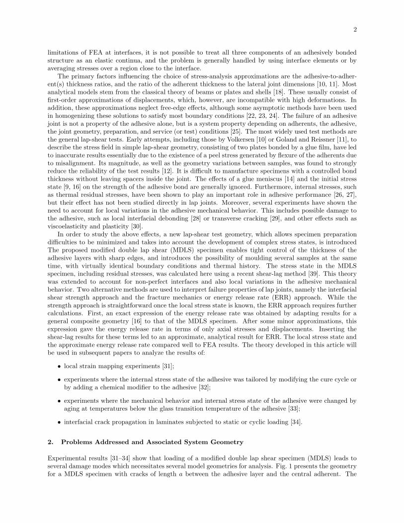
Experimental results [31–34] show that loading of a modified double lap shear specimen (MDLS) leads toseveral damage modes which necessitates several model geometries for analysis. Fig. 1 presents the geometryfor a MDLS specimen with cracks of length a between the adhesive layer and the central adherent. The

3 Compression Double Lap Shear Test I

2t1

t2

t3

a-L

σ0

t1

t3

σ0

t1

t3

σ0

σt

σt

x

z

ya

W

Fig. 1. Geometry of the modified double lap-shear specimen with cracks of length a between the adhesiveand the central adherent layer.

system is shown with 3 constituents: an inner plate of thickness 2t1, with Young’s modulus E1, Poisson’s ratioν1, and thermal expansion coefficient α1; two adhesive layers of thickness t2 and thermo-elastic propertiesE2, ν2, α2; and two outer plates of thickness t3 and thermo-elastic properties E3, ν3, α3. The boundaryconditions are defined by a compression stress of positive magnitude σ0 spread over the entire inner platewhile the two outer plates are simply supported. The top an bottom surfaces of the adhesive layer are notloaded or supported. Additionally, two lateral pressures (σt) can be applied on the outer adherents. Theorigin of the (x, y, z) axis system is in the middle of the specimen and aligned with the crack tip. The x axisis in the thickness direction while the y axis is in the loading direction.

The specimen geometry is symmetrical about the midplane, which means only half the specimen needsto be analyzed (see Fig. 2). The inner plate is labeled 1, the adhesive layer 2, and the outer plate 3. Thewidth of the specimen W is assumed large enough to be in plane stress conditions in the z = 0 plane ofthe specimen. This will be verified in the experimental part of this work by examining the fracture surfacesof the specimen [32–34]. The shear-lag analysis consists of determining the three averaged axial stresses⟨

σ(1)yy

⟩

,⟨

σ(2)yy

⟩

,⟨

σ(3)yy

⟩

in the layers, and the interfacial shear stresses τ(1)xy (at the layer 1/layer 2 interface),

τ(2)xy (at the layer 2/layer 3 interface). The shear stress at the midplane (τ

(0)xy ) and on the lateral surface

(τ(3)xy ) are zero by symmetry or by boundary conditions. The calculation of the energy release rate required

determination of the average displacements in the y direction < v(i) > in the system. These could also befound by the shear-lag analysis.

From experimental results [31–34], it was determined that four problems need to be addressed: i. the

4

t1

t2

t3

x

y

σ0

σ0

t1

t3

E2

I

E2

II

d

d-L

0

ZONE Itransversely

damaged

zone

ZONE IIElastic zone

t1

t2

t3

x

y

σ0

σ0

t1

t3

E2

II

d

d-L

0

ZONE Iyielded zone

ZONE IIElastic zone

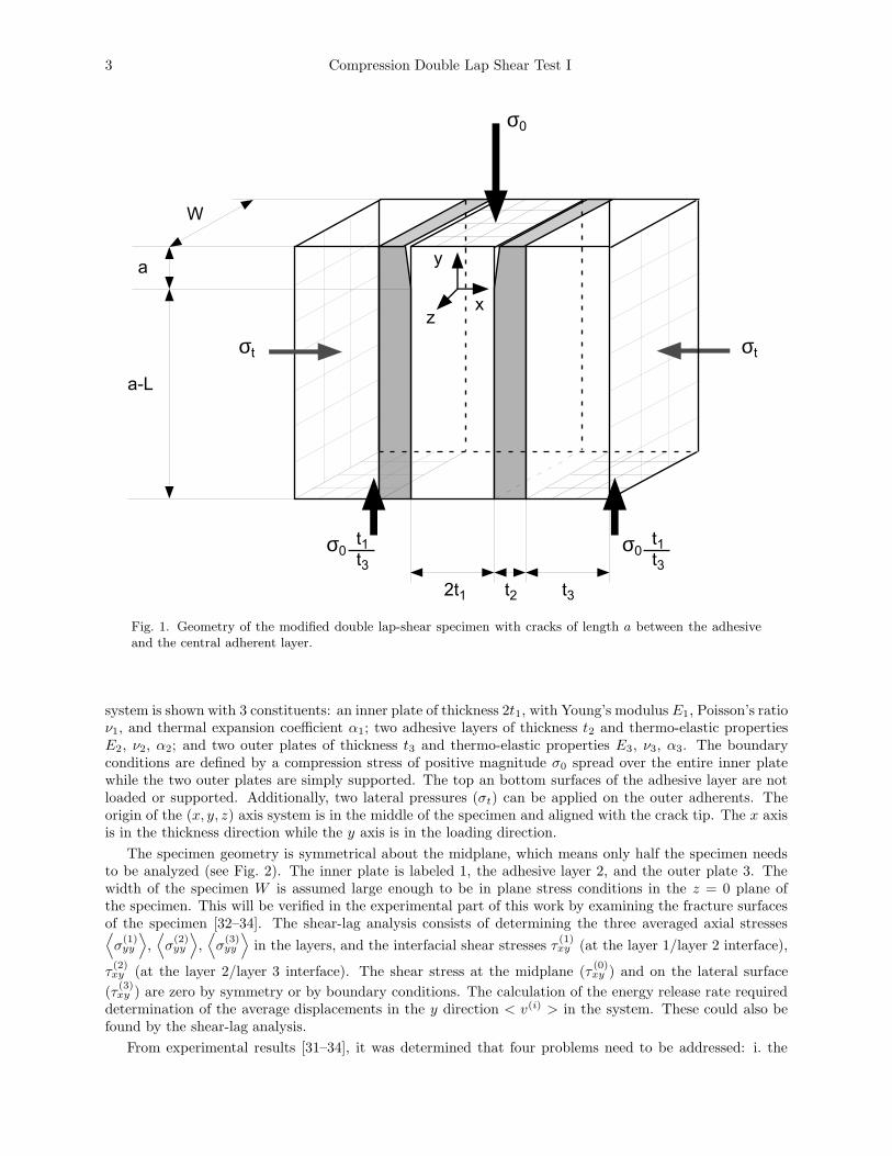
Fig. 2. Geometry of the MDLS specimen with a damaged zone of length d in the adhesive and 2 zones (Iand II) for the analysis. The damage zone can be a transversely cracked adhesive or a yielded adhesive

specimen fails in the elastic regime, ii. the adhesive mechanical properties are degraded locally prior tofailure, iii. the adhesive partially yields prior to adhesive failure, and iv. a crack propagates at the interfacebetween the inner plate and the adhesive. The first problem can be solved by a strength analysis using theshear-lag analysis. The three others are complicated if all local dissipative phenomena are to be accountedfor. Instead, we used a global approach: the properties of a transversely damaged zone or of a yielded zonewere averaged over the damage or yield length d (Fig. 2).

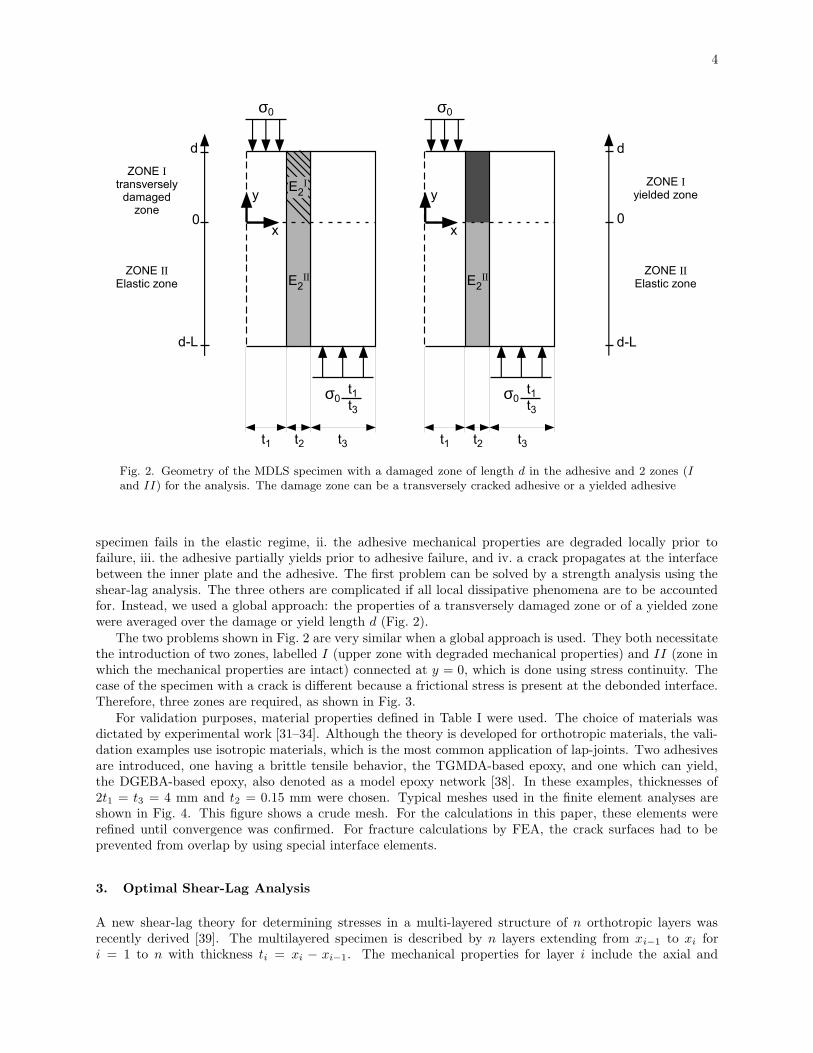
The two problems shown in Fig. 2 are very similar when a global approach is used. They both necessitatethe introduction of two zones, labelled I (upper zone with degraded mechanical properties) and II (zone inwhich the mechanical properties are intact) connected at y = 0, which is done using stress continuity. Thecase of the specimen with a crack is different because a frictional stress is present at the debonded interface.Therefore, three zones are required, as shown in Fig. 3.

For validation purposes, material properties defined in Table I were used. The choice of materials wasdictated by experimental work [31–34]. Although the theory is developed for orthotropic materials, the vali-dation examples use isotropic materials, which is the most common application of lap-joints. Two adhesivesare introduced, one having a brittle tensile behavior, the TGMDA-based epoxy, and one which can yield,the DGEBA-based epoxy, also denoted as a model epoxy network [38]. In these examples, thicknesses of2t1 = t3 = 4 mm and t2 = 0.15 mm were chosen. Typical meshes used in the finite element analyses areshown in Fig. 4. This figure shows a crude mesh. For the calculations in this paper, these elements wererefined until convergence was confirmed. For fracture calculations by FEA, the crack surfaces had to beprevented from overlap by using special interface elements.

3. Optimal Shear-Lag Analysis

A new shear-lag theory for determining stresses in a multi-layered structure of n orthotropic layers wasrecently derived [39]. The multilayered specimen is described by n layers extending from xi−1 to xi fori = 1 to n with thickness ti = xi − xi−1. The mechanical properties for layer i include the axial and


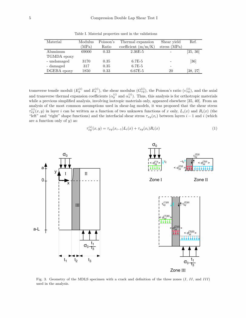
Table I. Material properties used in the validations

Material Modulus Poisson’s Thermal expansion Shear yield Ref.(MPa) Ratio coefficient (m/m/K) stress (MPa)

Aluminum 69000 0.33 2.36E-5 - [35, 36]TGMDA epoxy- undamaged 3170 0.35 6.7E-5 - [36]- damaged 317 0.35 6.7E-5 -DGEBA epoxy 1850 0.33 6.67E-5 20 [38, 27]

transverse tensile moduli (E(i)y and E

(i)x ), the shear modulus (G

(i)xy), the Poisson’s ratio (υ

(i)xy ), and the axial

and transverse thermal expansion coefficients (α(i)y and α

(i)x ). Thus, this analysis is for orthotropic materials

while a previous simplified analysis, involving isotropic materials only, appeared elsewhere [35, 40]. From ananalysis of the most common assumptions used in shear-lag models, it was proposed that the shear stress

τ(i)xy (x, y) in layer i can be written as a function of two unknown functions of x only, Li(x) and Ri(x) (the

“left” and “right” shape functions) and the interfacial shear stress τxy(xi) between layers i− 1 and i (whichare a function only of y) as:

τ (i)xy (x, y) = τxy(xi−1)Li(x) + τxy(xi)Ri(x) (1)

I

t1

t2

t3

x

y

σ0

σ0

t1

t3

a

a-L

0

II

III

σ0

t1

t3

Zone I

σ0

Zone II

Zone III

< σyy

>(3)III

< σyy

>(1)I

< σyy

>

(2)II< σ

yy >

(3)II

< σyy

>(1)III

< σyy

>(2)III

τxy

(1)III τxy

(2)III

τxy

(2)II

τf

−τf

Fig. 3. Geometry of the MDLS specimen with a crack and definition of the three zones (I, II, and III)used in the analysis.

6

Undamage Interface Cracked Interface

Fig. 4. Meshes used in the finite element analysis for specimens with an undamaged interface or ones withan interfacial crack. For clarity, the adhesive layer is shown thicker than in the actual specimens and not allelements are shown. The converged FEA calculations subdivided each of these elements about three times.


with

Li (x) =

{

1 at x = xi−1

0 at x = xi(2a)

Ri (x) =

{

0 at x = xi−1

1 at x = xi(2b)

Defining τ = (τxy(x1), τxy(x2), . . . , τxy(xn−1)), the shear-lag analysis can be reduced to a system of (n − 1)differential equations in terms of the (n− 1) unknown interfacial shear stresses [39]:

[A]∂2τ

∂y2− [B]τ = −τ0 (3)

where [A] and [B] are both tridiagonal matrices with elements:

Ai,i−1 =ti〈ξiLi〉

G(i)xy

, Ai,i =ti+1〈(1− ξi+1)Li+1〉

G(i+1)xy

+ti〈ξiRi〉

G(i)xy

, Ai,i+1 =ti+1〈(1− ξi+1)Ri+1〉

G(i+1)xy

(4)

Bi,i−1 = − 1

E(i)y ti

, Bi,i =1

E(i+1)y ti+1

+1

E(i)y ti

, Bi,i+1 = − 1

E(i+1)y ti+1

Here, the dimensionless coordinate in layer i is defined by

ξi =x− xi−1

ti(5)

The right side of the equation is defined by:

τ0 =

(

τ0

E(1)y t1

, 0, . . . ,τn

E(n)y tn

)

(6)

where τ0 and τn are the shear stresses in the middle of the specimen and on the free surface. For allcalculations in this paper, except one, these shear stress boundary conditions are zero.

For solution purposes, Eq. (3) is rewritten as:

∂2τ

∂y2− [Mτ ]τ = −[Mτ ][B]−1τ0 (7)

where [Mτ ] = [A]−1[B]. The solution of Eq. (7) is found by an eigen-analysis [39]:

τxy(xi) = τ0 +

i∑

j=1

tjE(j)y

tE(0)y

(τn − τ0) +

n−1∑

j=1

(

ajeλjy − bje

−λjy)

ωj,i (8)

where t =∑n

i=1 ti is the semi-thickness of the composite, E(0)y = 1

t

∑ni=1 tiE

(i)y is the rule-of-mixtures

effective composite modulus of an undamaged structure in the y direction, λ2j for j = 1 to n − 1 are the

eigenvalues of the [Mτ ] matrix, ωj,i is the ith element of the eigenvector of [Mτ ] associated with λ2j , and aj

and bj for j = 1 to n− 1 are constants to be determined by boundary conditions. Note that internal stressesdo not appear explicitly in this equation, but are included through aj and bj , calculated as shown below.Additionally, by making use of the equation of equilibrium, it was shown that the average axial stresses areobtained from:

〈σ(i)yy 〉 = E(i)

y

[

(τ0 − τn) + tσ0(0)

tE(0)y

+ (α(0)y − α(i)

y )∆T

]

+n−1∑

j=1

(

ajeλjy + bje

−λjy) ωj,i−1 − ωj,i

tiλj(9)

where α(0)y is the rule-of-mixtures, effective y-direction thermal expansion coefficient of an undamaged struc-

ture given by:

α(0)y =

n∑

i=1

α(i)y tiE

(i)y

tE(0)y

(10)

8

Note that σ0(y) = (τ0 − τn)y + σ0(0) is the total applied axial stress in the y-direction for problems withconstant, non-zero shear stresses applied to the sides of the specimen. When there are no shear-stressboundary conditions, σ0(y) is constant and equal to the total applied axial stress.

The average displacements in the y-direction in each layer i can be obtained as a function of the axialdisplacement at the interface xi or at xi+1, using [39]:

〈vi〉 = v(xi)−tiτxy(xi−1)

G(i)xy

〈ξiLi〉 −tiτxy(xi)

G(i)xy

〈ξiRi〉 (11)

The average displacement difference across layer i is thus [39]:

〈vi+1〉 − 〈vi〉 =ti+1〈(1− ξi+1)Ri+1〉

G(i+1)xy

τxy(xi+1) +ti〈ξiLi〉

G(i)xy

τxy(xi−1) (12)

+

(

ti+1〈(1− ξi+1)Li+1〉G

(i+1)xy

+ti〈ξiRi〉

G(i)xy

)

τxy(xi)

In the following sections these equations are applied to several different analyzes of the MDLS specimen.

4. Strength Approach

4.1. Specimen Failing in the Linear-Elastic Region

4.1.1. Stress Analysis Solution Method

For a specimen failing in the linear-elastic region, we eliminated the crack and used the modified shear-lag

theory with n = 3 layers. The interfacial shear (τ(i)xy = τxy(xi)) and average axial stresses (〈σ(i)

yy 〉) are givenby [39]:

τ (1)xy =

(

a1eλ1y − b1e

−λ1y)

ω1,1 +(

a2eλ2y − b2e

−λ2y)

ω2,1

τ (2)xy =

(

a1eλ1y − b1e

−λ1y)

ω2,1 +(

a2eλ2y − b2e

−λ2y)

ω2,2

〈σ(1)yy 〉 = C1 −

(

a1eλ1y + b1e

−λ1y) ω1,1

λ1t1−(

a2eλ2y + b2e

−λ2y) ω2,1

λ2t1(13)

〈σ(2)yy 〉 = C2 −

(

a1eλ1y + b1e

−λ1y) ω1,2 − ω1,1

λ1t2−(

a2eλ2y + b2e

−λ2y) ω2,2 − ω2,1

λ2t2

〈σ(3)yy 〉 = C3 +

(

a1eλ1y + b1e

−λ1y) ω1,2

λ1t3+(

a2eλ2y + b2e

−λ2y) ω2,2

λ2t3

where the constants Ci define the far-field stress state (i.e., the stresses far away from specimen ends andcracks) and are given by:

Ci = E(i)y

(

− t1σ0

tE(0)y

+ (α(0)y − α(i)

y )∆T

)

(14)

Here σy(0) = −σ0 where σ0 is the positive magnitude of the applied compressive stress. The remainingconstants, aj and bj , j = 1, 2, were determined by the boundary conditions on the average axial stress inthe inner adherent and the adhesive layer. With the origin of the system at the middle of the specimen, theboundary conditions are:

〈σ(1)yy 〉∣

∣

∣

y=L/2= −σ0; 〈σ(1)

yy 〉∣

∣

∣

y=−L/2= 0; 〈σ(2)

yy 〉∣

∣

∣

y=±L/2= 0 (15)

The average axial stress in the layer 3 is given by force balance. Solving for the four unknowns a1, a2, b1, b2


as functions of C1 and C2 gives:

a1 =σ0e4

(

sinh(

λ1L2

)

+ cosh(

λ1L2

))

− 2 (e2C2 − e4C1) sinh(

λ1L2

)

2 (e1e4 − e2e3) sinh (λ1L)

b1 =σ0e4

(

sinh(

λ1L2

)

− cosh(

λ1L2

))

− 2 (e2C2 − e4C1) sinh(

λ1L2

)

2 (e1e4 − e2e3) sinh (λ1L)

a2 =σ0e3

(

sinh(

λ2L2

)

+ cosh(

λ2L2

))

− 2 (e1C2 − e3C1) sinh(

λ2L2

)

2 (e2e3 − e1e4) sinh (λ2L)(16)

b2 =σ0e3

(

sinh(

λ2L2

)

− cosh(

λ2L2

))

− 2 (e1C2 − e3C1) sinh(

λ2L2

)

2 (e2e3 − e1e4) sinh (λ2L)

where

e1 =ω1,1

λ1t1; e2 =

ω2,1

λ2t1; e3 =

ω1,2 − ω1,1

λ1t2; e4 =

ω2,2 − ω2,1

λ2t2(17)

The obtained set of equations presents a full, closed form solution of both axial and shear stresses in theMDLS sample. This solution depends upon the choice of shape functions which enter in the definition ofmatrix [A]. For a three-layer problem, the final solution depends only on six dimensionless averages of theshape function in the layers, namely 〈ζ1R1〉 , 〈(1− ζ2) L2〉 , 〈(1− ζ2) R2〉 , 〈ζ2L2〉 , 〈ζ2R2〉 and 〈(1− ζ3) L3〉.

4.1.2. The Influence of Shape Functions

The solution in the previous section was compared to FEA results for various shape functions. A commonassumption in prior shear-lag methods is to take all shape function as linear, which implies Li = 1− ξi andRi = ξi. The required averages reduce to

〈ξiLi〉 =1

6; 〈(1− ξi)Li〉 =

1

3; 〈ξiRi〉 =

1

3; 〈(1− ξi)Ri〉 =

1

6(18)

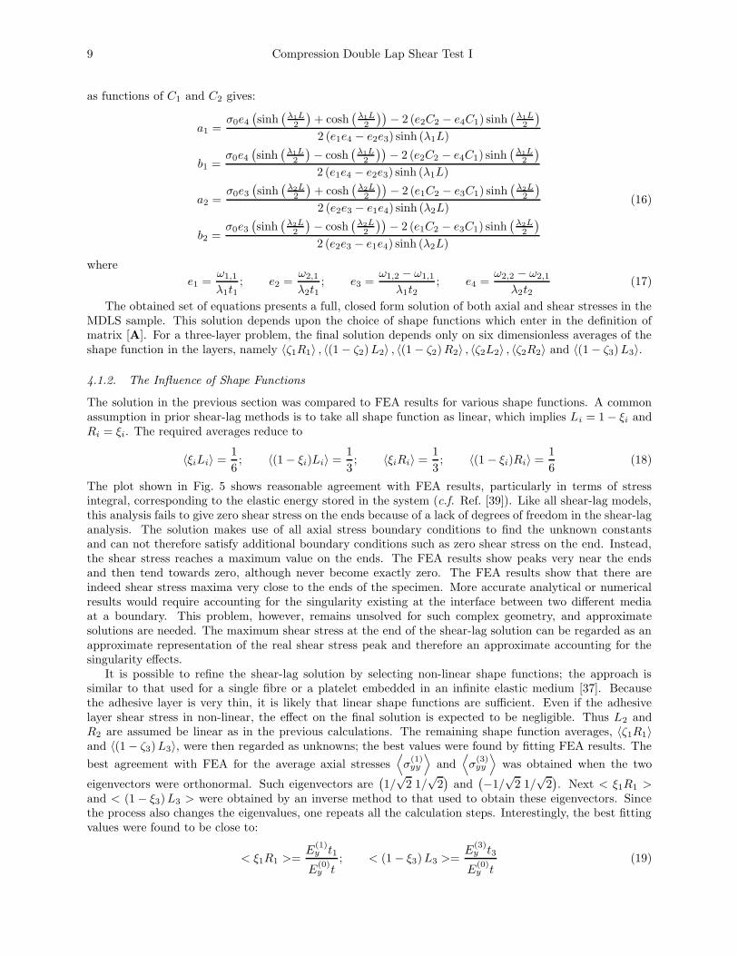
The plot shown in Fig. 5 shows reasonable agreement with FEA results, particularly in terms of stressintegral, corresponding to the elastic energy stored in the system (c.f. Ref. [39]). Like all shear-lag models,this analysis fails to give zero shear stress on the ends because of a lack of degrees of freedom in the shear-laganalysis. The solution makes use of all axial stress boundary conditions to find the unknown constantsand can not therefore satisfy additional boundary conditions such as zero shear stress on the end. Instead,the shear stress reaches a maximum value on the ends. The FEA results show peaks very near the endsand then tend towards zero, although never become exactly zero. The FEA results show that there areindeed shear stress maxima very close to the ends of the specimen. More accurate analytical or numericalresults would require accounting for the singularity existing at the interface between two different mediaat a boundary. This problem, however, remains unsolved for such complex geometry, and approximatesolutions are needed. The maximum shear stress at the end of the shear-lag solution can be regarded as anapproximate representation of the real shear stress peak and therefore an approximate accounting for thesingularity effects.

It is possible to refine the shear-lag solution by selecting non-linear shape functions; the approach issimilar to that used for a single fibre or a platelet embedded in an infinite elastic medium [37]. Becausethe adhesive layer is very thin, it is likely that linear shape functions are sufficient. Even if the adhesivelayer shear stress in non-linear, the effect on the final solution is expected to be negligible. Thus L2 andR2 are assumed be linear as in the previous calculations. The remaining shape function averages, 〈ζ1R1〉and 〈(1− ζ3) L3〉, were then regarded as unknowns; the best values were found by fitting FEA results. The

best agreement with FEA for the average axial stresses⟨

σ(1)yy

⟩

and⟨

σ(3)yy

⟩

was obtained when the two

eigenvectors were orthonormal. Such eigenvectors are(

1/√

2 1/√

2)

and(

−1/√

2 1/√

2)

. Next < ξ1R1 >and < (1− ξ3) L3 > were obtained by an inverse method to that used to obtain these eigenvectors. Sincethe process also changes the eigenvalues, one repeats all the calculation steps. Interestingly, the best fittingvalues were found to be close to:

< ξ1R1 >=E

(1)y t1

E(0)y t

; < (1− ξ3) L3 >=E

(3)y t3

E(0)y t

(19)

10

-10 -5 0 5 10

-1.0

-0.8

-0.6

-0.4

-0.2

0.0

0.2

0.4

optimal shape functions

linear shape

functions

linear shape

functions

Distance Along Lap-Joint y (mm)

S

tre

ss (M

P

a

)

σyy

(1)

σyy

(3)

τxy

(1)

Fig. 5. Axial and shear stresses vs. distance along lap-joint, linear and optimal shape function solutions(TGMDA-based epoxy adhesive, stresses are normalized vs. σ0, and ∆T = 0)

In other words, the optimal shape function averages were equal to the fraction of the specimen stiffnesscontributed by that layer.

Figure 5 plots the stresses obtained using optimal shape function, in comparison to those obtained withlinear shape functions. The solution is improved by the use of refined shape functions. The average axialstresses in the adherents are nearly exact to the FEA results. The shear stress calculation is improved butstill has the limitation of all shear-lag models of maximum shear stress on the ends instead of zero shearstress. It should be noted that FEA results do not provide an exact solution either, since this method doesnot deal with interfaces in a continuous way, i.e., stresses and their derivatives are non continuous across theinterface. Therefore, the optimal shear-lag method presented here, representing the best shear-lag solution,together with the use of its shape functions, is believed to be accurate on the level of FEA results to serveas a basis for further investigations.

The plots show average axial stresses and shear stresses. Shear lag can also find average axial displace-ments and they similarly agree with FEA results. Shear lag has used to find other terms, such as transversestresses or displacements, bu such results are not accurate [39]. In fracture mechanics calculations, it isnecessary to find total strain energy in the specimen. Because the strain energy in the MDLS specimencan be found using boundary integrals and reduced to a result that depends only on axial stresses anddisplacements, this energy can be found accurately by shear-lag analysis [39].


-10 -5 0 5 10

-50

-40

-30

-20

-10

0

10

20

Distance Along Lap-Joint (mm)

A

xia

l S

tre

ss (M

P

a

)

σyy

(2), ∆T=-100°C

σyy

(2), ∆T=0

σyy

(1), ∆T=-100°C

σyy

(3), ∆T=-100°C

σyy

(3), ∆T=0

σyy

(1), ∆T=0

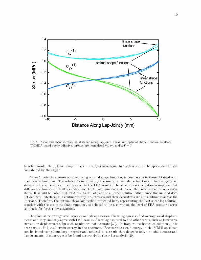
Fig. 6. Axial stresses vs. distance along a lap-joint, TGMDA-based epoxy adhesive, solution with hyperbolicshape functions, including internal stresses as indicated on the figure by ∆T , σ0 = 50 MPa.

4.1.3. Influence of Internal Stresses

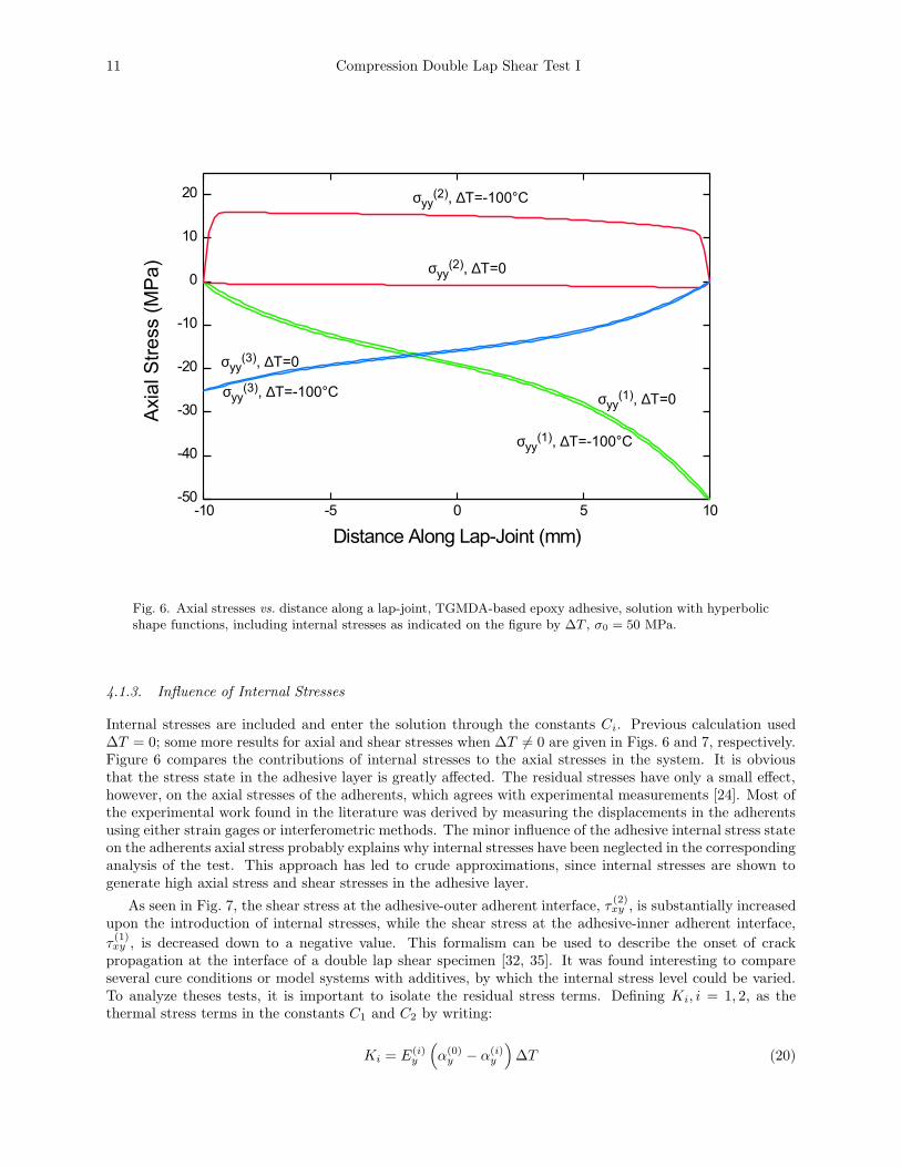
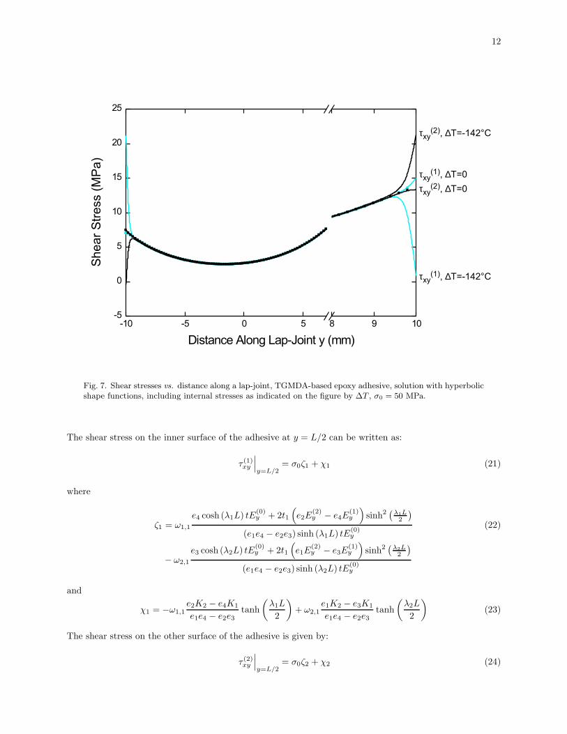
Internal stresses are included and enter the solution through the constants Ci. Previous calculation used∆T = 0; some more results for axial and shear stresses when ∆T 6= 0 are given in Figs. 6 and 7, respectively.Figure 6 compares the contributions of internal stresses to the axial stresses in the system. It is obviousthat the stress state in the adhesive layer is greatly affected. The residual stresses have only a small effect,however, on the axial stresses of the adherents, which agrees with experimental measurements [24]. Most ofthe experimental work found in the literature was derived by measuring the displacements in the adherentsusing either strain gages or interferometric methods. The minor influence of the adhesive internal stress stateon the adherents axial stress probably explains why internal stresses have been neglected in the correspondinganalysis of the test. This approach has led to crude approximations, since internal stresses are shown togenerate high axial stress and shear stresses in the adhesive layer.

As seen in Fig. 7, the shear stress at the adhesive-outer adherent interface, τ(2)xy , is substantially increased

upon the introduction of internal stresses, while the shear stress at the adhesive-inner adherent interface,

τ(1)xy , is decreased down to a negative value. This formalism can be used to describe the onset of crack

propagation at the interface of a double lap shear specimen [32, 35]. It was found interesting to compareseveral cure conditions or model systems with additives, by which the internal stress level could be varied.To analyze theses tests, it is important to isolate the residual stress terms. Defining Ki, i = 1, 2, as thethermal stress terms in the constants C1 and C2 by writing:

Ki = E(i)y

(

α(0)y − α(i)

y

)

∆T (20)

12

-10 -5 0 5 8 9 10

-5

0

5

10

15

20

25


S

h

e

a

r S

tre

ss (M

P

a

)

τxy

(2), ∆T=-142°C

τxy

(2), ∆T=0

τxy

(1), ∆T=0

τxy

(1), ∆T=-142°C

Fig. 7. Shear stresses vs. distance along a lap-joint, TGMDA-based epoxy adhesive, solution with hyperbolicshape functions, including internal stresses as indicated on the figure by ∆T , σ0 = 50 MPa.

The shear stress on the inner surface of the adhesive at y = L/2 can be written as:

τ (1)xy

∣

∣

∣

y=L/2= σ0ζ1 + χ1 (21)

where

ζ1 = ω1,1

e4 cosh (λ1L) tE(0)y + 2t1

(

e2E(2)y − e4E

(1)y

)

sinh2(

λ1L2

)

(e1e4 − e2e3) sinh (λ1L) tE(0)y

(22)

− ω2,1


(

e1E(2)y − e3E

(1)y

)

sinh2(

λ2L2

)


and

χ1 = −ω1,1e2K2 − e4K1

e1e4 − e2e3tanh

(

λ1L

2

)

+ ω2,1e1K2 − e3K1

e1e4 − e2e3tanh

(

λ2L

2

)

(23)

The shear stress on the other surface of the adhesive is given by:

τ (2)xy

∣

∣

∣

y=L/2= σ0ζ2 + χ2 (24)


where

ζ2 = ω1,2


(

e2E(2)y − e4E

(1)y

)

sinh2(

λ1L2

)


(25)

− ω2,2


(

e1E(2)y − e3E

(1)y

)

sinh2(

λ2L2

)


and

χ2 = −ω1,2e2K2 − e4K1

e1e4 − e2e3tanh

(

λ1L

2

)

+ ω2,2e1K2 − e3K1

e1e4 − e2e3tanh

(

λ2L

2

)

(26)

This formulation is useful because it splits the apparent interfacial shear strength for applied mechanicalloads into internal stress effects and the true shear stresses required for debonding. Writing the experimentalshear stress at failure in terms of the applied compression stress as

τexp =F

2WL= σ0

t1L

(27)

one obtains at failure:

τ (1)xy

∣

∣

∣

y=L/2= τ0 = τexp

L

t1ζ1 + χ1 (28)

⇒ τexp =t1

Lζ1(τ0 − χ1) (29)

or, if debonding starts on the other interface:

τexp =t1

Lζ2(τ0 − χ2) (30)

In this formalism, τ0 represents the true, local shear strength of the interface, which does not depend oninternal stresses or on the geometry. In contrast, the observed experimental shear strength, τexp, is affectedboth by interfacial properties and by residual stresses effects. In brief, τ0 is the more fundamental propertyfor characterization of the interface. This simplified analysis was found to be robust enough to analyzeexperimental data for the onset of debonding, when the specimen failed in the linear-elastic regime.

4.2. Stresses in a Transversely Cracked Specimen

The problem of stresses when the adhesive is damaged by transverse cracks arises from experimental obser-vations in Ref. [32]. It was observed that some brittle epoxy adhesives transversely crack prior to debonding.The extent of transverse cracking was reproducible. This section establishes the equations necessary for de-scribing this phenomenon. Consider a damaged zone of length d as shown in Fig. 2. As a first approximation,we considered that the shear modulus of the adhesive, and thereby its Young’s modulus too, were reduced bytransverse cracking. This hypothesis was well supported by the stress-strain curves obtained during loadingof the MDLS specimen, which showed a decrease of the effective modulus of the joint. Using this hypothesis,the stresses of the system could be found by analyzing two zones with distinct mechanical properties for theadhesive, and making axial and shear stresses continuous across the two zones. The stress in the two zonesare each given by Eq. (13) except that separate constants are needed for each zone or aj → ak

j , bj → bkj ,

Cj → Ckj , ωj,i → ωk

j,i, and λj → λkj where k = I, II . The constants Ck

j are given by Eq. (14) using E(i)ky

and α(i)ky for layer properties and rule-of-mixtures results redefined as

E(0)ky =

E(1)y t1 + E

(2)ky t2 + E

(3)y t3

t(31)

α(0)ky =

α(1)y E

(1)y t1 + α

(2)y E

(2)ky t2 + α

(3)y E

(3)y t3

tE(0)ky

(32)

14

Notice that only the mechanical properties of layer 2 differ between zones I and II. The eight unknownconstants, ak

j , bkj with j = 1, 2 were obtained from the following the eight boundary conditions:

⟨

σ(2)Iyy

⟩∣

∣

∣

y=d= 0;

⟨

σ(2)IIyy

⟩∣

∣

∣

y=d−L= 0;

⟨

σ(1)Iyy

⟩∣

∣

∣

y=d= −σ0

⟨

σ(1)IIyy

⟩∣

∣

∣

y=d−L= 0;

⟨

σ(2)Iyy

⟩∣

∣

∣

y=0=⟨

σ(2)IIyy

⟩∣

∣

∣

y=0;

⟨

σ(1)Iyy

⟩∣

∣

∣

y=0=⟨

σ(1)IIyy

⟩∣

∣

∣

y=0(33)

τ (1)Ixy

∣

∣

∣

y=0= τ (1)II

xy

∣

∣

∣

y=0; τ (2)I

xy

∣

∣

∣

y=0= τ (2)II

xy

∣

∣

∣

y=0

Figure 8 shows the distribution of stresses in the adhesive joint submitted to internal stresses and applied

stress, considering a fragmented zone of length d = 3 mm in which E(i)Iy = 0.1E

(1)IIy or damage caused 90%

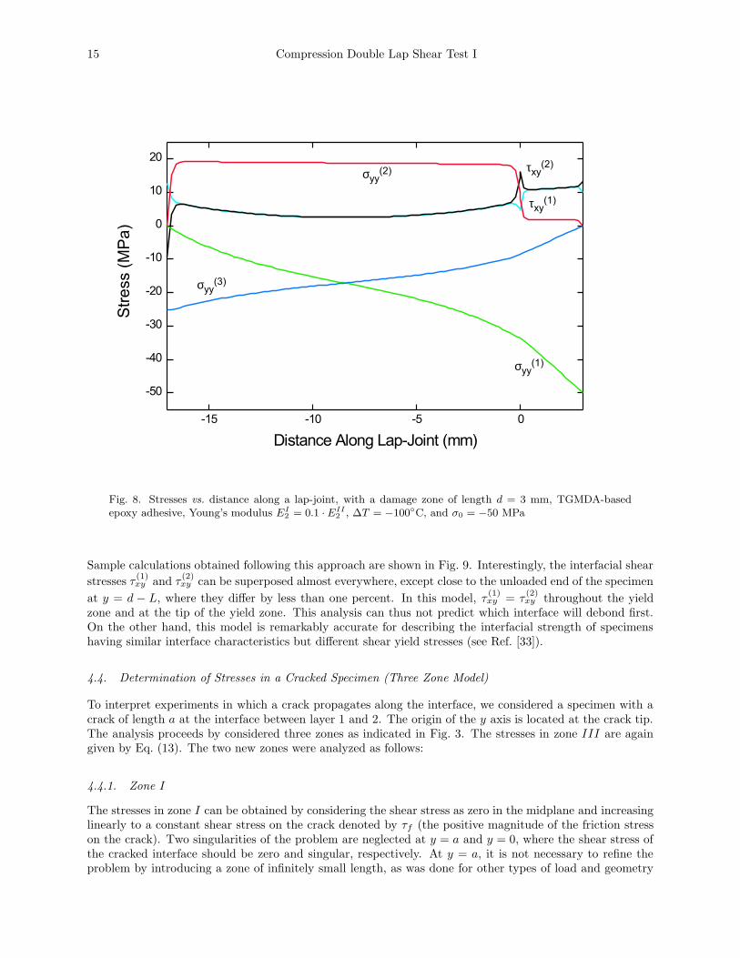
degradation. This value was set arbitrarily, based on those obtained from fitting the force vs. displacementcurves of TGMDA-based specimens used in experiments detailed elsewhere [32]. It will be further shownthat the experimental stress-strain curve is modelled accurately by the present theory, the major difficultybeing the determination of the onset of transverse microcracking. On this plot the two zones connected atthe origin y = 0 clearly appear, and they involve a local reduction of the axial tensile stress in the damagedadhesive which is essentially due to Young’s modulus reduction and the release of internal stresses it induces.The shear stress profiles are still influenced by internal stresses, which involve a stress increase at the loadedend of the specimen (y = 3 on Fig. 8).

More information than available would be needed to accurately calculate the modulus reduction in thefragmented zone: the angle of the transverse crack with the interface plane is usually observed to be close to45◦, but some variations were observed between specimens with different internal stress states; the distancebetween two consecutive fragments would also provide useful information on the rate of the damage prop-agation. As a consequence, the present analysis, which uses an average loss of mechanical properties, is afirst approximation of the fracture mechanics involved in the process. Accurate modelling of the local stressstate and fracture mechanics involving fragmentation nucleation, propagation, as well as the friction betweenfragments, would better describe the residual properties of the fragmented adhesive zone. Nevertheless, oneof the attractive features of this model is to quantify the fracture process efficiently by describing initiation,propagation and first adhesive failure of the joint, as will be illustrated by experimental results in Ref. [32].

4.3. Specimen with a Partially Yielded Adhesive

For this analysis, the adhesive was considered as a time-independent, elastic-perfectly-plastic material. Vis-coelastic relaxation of internal stresses can be included by using an effective temperature step, as describedin Ref. [33]. One can then model the MDLS specimen as two connected zones with different properties(Fig. 2): a first zone in which the adhesive yields and which is characterized by a constant shear stress,connected to a second zone in which the adhesive has an elastic behavior. This case resembles the previousone, in which zone I had altered properties. One major difference arises: for a yielded interface, the yieldstress can be evaluated experimentally while it is more difficult to determine the correct results to use for adegraded modulus.

In this analysis, the shear stress in zone I is a constant τp equal to the shear yield stress of the adhesive,which leads to zone I stress state of:

τ (1)Ixy = τ (2)I

xy = τp; 〈σ(1)Iyy 〉 =

τp

t1(d− y)− σ0; 〈σ(3)I

yy 〉 =τp

t3(y − d) (34)

Because the shear stress in layer 2 is constant (and also by force balance), the average stress in the adhesive

in zone I (〈σ(2)Iyy 〉) is zero. The zone II stress state is again given by Eq. (13). The boundary conditions for

the four unknowns in zone II involve the continuity of axial stresses between the two zones, and the freeend conditions:

〈σ(1)Iyy 〉

∣

∣

∣

y=0= 〈σ(1)II

yy 〉∣

∣

∣

y=0; 〈σ(1)II

yy 〉∣

∣

∣

y=d−L= 0 (35)

〈σ(2)Iyy 〉

∣

∣

∣

y=0= 〈σ(2)II

yy 〉∣

∣

∣

y=0= 0; 〈σ(2)II

yy 〉∣

∣

∣

y=d−L= 0


-15 -10 -5 0

-50

-40

-30

-20

-10

0

10

20

Distance Along Lap-Joint (mm)

S

tre

ss (M

P

a

)

σyy

(2)

σyy

(3)

σyy

(1)

τxy

(2)

τxy

(1)

Fig. 8. Stresses vs. distance along a lap-joint, with a damage zone of length d = 3 mm, TGMDA-basedepoxy adhesive, Young’s modulus E

I2 = 0.1 · EII

2 , ∆T = −100◦C, and σ0 = −50 MPa

Sample calculations obtained following this approach are shown in Fig. 9. Interestingly, the interfacial shear

stresses τ(1)xy and τ

(2)xy can be superposed almost everywhere, except close to the unloaded end of the specimen

at y = d − L, where they differ by less than one percent. In this model, τ(1)xy = τ

(2)xy throughout the yield

zone and at the tip of the yield zone. This analysis can thus not predict which interface will debond first.On the other hand, this model is remarkably accurate for describing the interfacial strength of specimenshaving similar interface characteristics but different shear yield stresses (see Ref. [33]).

4.4. Determination of Stresses in a Cracked Specimen (Three Zone Model)

To interpret experiments in which a crack propagates along the interface, we considered a specimen with acrack of length a at the interface between layer 1 and 2. The origin of the y axis is located at the crack tip.The analysis proceeds by considered three zones as indicated in Fig. 3. The stresses in zone III are againgiven by Eq. (13). The two new zones were analyzed as follows:

4.4.1. Zone I

The stresses in zone I can be obtained by considering the shear stress as zero in the midplane and increasinglinearly to a constant shear stress on the crack denoted by τf (the positive magnitude of the friction stresson the crack). Two singularities of the problem are neglected at y = a and y = 0, where the shear stress ofthe cracked interface should be zero and singular, respectively. At y = a, it is not necessary to refine theproblem by introducing a zone of infinitely small length, as was done for other types of load and geometry

16

-15 -10 -5 0 5

-200

-150

-100

-50

0

50


-15 -10 -5 0 5

-2

-1

0

1

2

3

4

S

tre

ss (M

P

a

)

σyy

(2)

σyy

(3)

σyy

(1)

τxy

(1)

Fig. 9. Stresses vs. distance along a lap-joint, DGEBA-based epoxy adhesive, solution with hyperbolic shapefunctions, including constant shear stress τp = 20 MPa in the yielded zone, σ0 = 200 MPa, ∆T = −15◦C.

[41, 42, 43], because the ERR does not depend on the shear stress τxy(a). The singularity at y = 0 is moreof a problem, and the accuracy of the model should be checked at that location.

Force equilibrium on an element of length dy leads to (see Ref. [39] for details):

∂⟨

σ(1)Iyy

⟩

∂y= −τf

t1(36)

Using the boundary condition:⟨

σ(1)Iyy

⟩∣

∣

∣

y=a= −σ0 (37)

the zone I axial stress is:⟨

σ(1)Iyy

⟩

= τfa− y

t1− σ0 (38)

4.4.2. Zone II

In zone II , the friction stress in the debonded interface is of opposite sign to that of zone I , and thereforeequals −τf . This case corresponds to a two-layer, shear-lag analysis with non-zero boundary shear stress. Itcan be solved using the following equation [39]:

∂2τ(2)IIxy

∂y2− β2τ (2)II

xy =τf

E(2)y t2

1t2

3G(2)xy

+ t33G

(3)xy

(39)


where the optimal shear-lag parameter is

β2 =

1

E(2)y t2

+ 1

E(3)y t3

t23G

(2)xy

+ t33G

(3)xy

(40)

Solving Eq. (39), one obtains:

t2

⟨

σ(2)IIyy

⟩

= aIIeβy + bIIe−βy + E(2)y t2

(

τf (y − a)

E(0)IIy (t2 + t3)

+(

α(0)IIy − α(2)

y

)

∆T

)

t3

⟨

σ(3)IIyy

⟩

= −aIIeβy − bIIe−βy + E(3)y t3

(

τf (y − a)

E(0)IIy (t2 + t3)

+(

α(0)IIy − α(3)

y

)

∆T

)

(41)

τ (2)IIxy =

E(3)y t3τf

(t2 + t3) E(0)IIy

− βaIIeβy + βbIIe−βy

and E(0)IIy andα

(0)IIy are the rule-of-mixtures properties for the system with 2 layers, i.e.:

E(0)IIy =

E(2)y t2 + E

(3)y t3

t2 + t3(42)

α(0)IIy =

α(2)y E

(2)y t2 + α

(3)y E

(3)y t3

E(0)IIy (t2 + t3)

4.4.3. Boundary Conditions

The above stresses have six unknowns: aII , bII , aIII1 , bIII

1 , aIII2 , and bIII

2 . These unknowns were determinedfrom the following six boundary conditions:

⟨

σ(2)IIyy

⟩∣

∣

∣

y=a= 0;

⟨

σ(2)IIyy

⟩∣

∣

∣

y=0=⟨

σ(2)IIIyy

⟩∣

∣

∣

y=0;

⟨

σ(1)IIIyy

⟩∣

∣

∣

y=0= τfa− t1σ0 (43)

⟨

σ(1)IIIyy

⟩∣

∣

∣

y=a−L= 0;

⟨

σ(2)IIIyy

⟩∣

∣

∣

y=a−L= 0; τ III

2

∣

∣

y=0= τ II

2

∣

∣

y=0

As shown in Figs. 10 and 11, the stresses found by this analysis agree well with FEA results for a crackedspecimen.

5. Energy Release Rate

Using the stress state in the previous section, it is possible to calculate the energy release rate for growth of aninterfacial crack. The calculation of the energy release rate proceeds in two steps. First, an exact expressionfor the energy release rate which can be reduced to a result that depends only on axial displacements andaverage axial stresses is derived. Second, the shear-lag results for these displacements and stresses are usedto derive an approximate energy release rate.

5.1. Exact Results

A general result for energy release rate in composite fracture which includes residual stresses and tractionloads on cracks (e.g., friction) was recently derived as [16]:

G =1

2

∂

∂A

∫

S+Sc

~T 0.~udS +

∫

V

σα∆TdV

(44)

where A is the cracked area, S denotes the outer surface, Sc stands for the cracked surfaces, and V denotesthe volume. ~T 0 is the traction loads which are applied to S and possibly also on Sc, and ~u = (u, v, w)where the components are the displacements in the x, y, and z directions.

18

-15 -10 -5 0 5

-1.0

-0.8

-0.6

-0.4

-0.2

0.0

0.2


S

tre

ss (M

P

a

)

σyy

(2)

σyy

(3)

σyy

(1)

Fig. 10. Normalized axial stresses vs. distance along a lap-joint, TGMDA-based epoxy adhesive, solutionwith hyperbolic shape functions, including constant friction in debond zone (τf = 0.05σ0), ∆T = 0).

Table II. Calculation of the traction-displacement integrals for all loaded boundary surfaces and traction-loaded crack surfaces.

Surface ~T 0 ~u∫

S+Sc

~T 0.~udS

top plate 1 (0 − σ0 0) (u1 v1 (x, a) w1) −σ0t1W 〈v1 (a)〉bottom plate 3

(

0 σ0t1t3

0)

(u3 v3 (x, a) w3) σ0t1W 〈v3 (a− L)〉crack surface, plate 1 (−σt τf 0) (u1 (t1, y) v1 (t1, y) w1)crack surface, plate 2 (σt − τf 0) (u2 (t1, y) v2 (t1, y) w2)crack surfaces† W

∫ a

0 τf (v1 (t1, y)− v2 (t1, y)) dyside surface (−σt 0 0) (u3 (t, y) v3 w3) −σtLW 〈u3 (t)〉

† From the two preceding lines ~T 0 · ~u = −σtu1 (t1) + τfv1 (t1, y)− τfv2 (t1, y) + σtu2 (t1), but the transversestress terms cancel because either u1 (t1) = u2 (t1), when the crack surfaces are in contact, or σt = 0, whenthe crack surfaces are not in contact.


-15 -10 -5 0 5

0.00

0.05

0.10

0.15

0.20

0.25

0.30

0.35


S

tre

ss (M

P

a

)

τxy

(2)

τxy

(1)

Fig. 11. Normalized shear stresses vs. distance along a lap-joint, TGMDA-based epoxy adhesive, solutionwith hyperbolic shape functions, including constant friction in debond zone (τf = 0.05σ0, ∆T = 0).

The vectors ~T 0 and ~u on loaded surfaces and crack surfaces of the MDLS specimen and their contributionsto the surface integral are given in Table II. Here σt is the transverse stress, as shown in Fig. 1. Using theseresults with the crack area dA = W da, G can be recast as:

G =1

2W

d

da

[

−σ0t1W 〈v1 (a)〉+ σ0t1W 〈v3 (a− L)〉 − σtLW 〈u3 (t)〉 (45)

+W

∫ a

0

τf (v1 (t1, y)− v2 (t1, y)) dy +

∫

V

σα∆TdV

]

Simplifying the volume integral [16] leads to:

G =1

2

d

da

[

−σ0t1 〈v1 (a)〉+ σ0t1 〈v3 (a− L)〉 − σtL 〈u3 (t)〉 (46)

+

∫ a

0

τf (v1 (t1, y)− v2 (t1, y)) dy + L(

α(1)y − α(2)

y

)

∆T t1σ(1)yy + L

(

α(3)y − α(2)

y

)

∆T t3σ(3)yy

]

where the bars denote phase averaged stresses, calculated as:

σ(i)yy =

∫

Vi

σ(i)yy dv =

1

L

a∫

a−L

⟨

σ(i)yy

⟩

dy (47)

20

5.2. Approximate Solution

The expression for the energy release rate G determined by Eq. (46) is exact and depends only on axialstresses and displacements in the three layers. The optimal shear lag analysis is used in this section to geta approximate solution for G.

5.2.1. Calculation of Displacements in the 3 Zones

Zone I: In its most general form,

〈v1〉 = 〈v1(0)〉+

y∫

0

⟨

ε(1)yy

⟩

dy = 〈v1(0)〉+

y∫

0

(

σ(1)yy

E(1)y

+ α(1)y ∆T

)

dy (48)

The only approximation here is to ignore contributions of transverse stresses to the axial strain [39]. Takingas a reference for displacements 〈v1 (0)〉 = 0, and making use of Eq. (38), one obtains

〈v1〉 =y

t1E(1)y

(

τf (a− 1

2y)− σ0t1

)

+ α(1)y ∆Ty (49)

and therefore:

〈v1 (a)〉 =a

t1E(1)y

(

1

2τf a− σ0t1

)

+ α(1)y ∆Ta (50)

The edge displacement v1 (t1, y) also needs to be calculated. From Eq. (11):

v1 (t1, y) = 〈v1(y)〉+τf t1

G(1)xy

〈ξ1R1〉 =y

t1E(1)y

(

τf (a− 1

2y)− σ0t1

)

+ α(1)y ∆Ty +

τf

G(1)xy

t1 〈ξ1R1〉 (51)

Zone II: By a similar analysis:

〈v2〉 = 〈v2 (0)〉+

y∫

0

(

σ(2)yy

E(2)y

+ α(2)y ∆T

)

dy (52)

With 〈σ(2)IIyy 〉 given by Eq. (41):

〈v2〉 = 〈v2 (0)〉+aII(

eβy − 1)

βE(2)y t2

− bII(

e−βy − 1)

βE(2)y t2

+ τf

(

y2 − 2ay)

2 (t2 + t3) E(0)IIy

+ α(0)IIy ∆Ty (53)

To obtain the 〈v2 (0)〉 term, the edge displacement v2 (t1, y) needs to be calculated first. Again, from Eq. (11),and with accounting for shear stresses on the edges of zone II :

v2 (t1, y) = 〈v2(y)〉 − τ(2)IIxy (y)t2

G(2)xy

〈ξ2R2〉 −τf

G(2)xy

t2〈ξ2L2〉 (54)

The continuity of axial displacement between zones I and II at y = 0:

v2 (t1, 0) = v1 (t1, 0) (55)

yields

〈v2 (0)〉+τ

(2)xy (0)

G(2)xy

t2 〈ξ2R2〉 −τf

G(2)xy

t2 〈ξ2L2〉 =τf

G(1)xy

t1 〈ξ1R1〉 (56)

and

〈v2 (0)〉 =t2 〈ξ2R2〉

G(2)xy

(

βaII − βbII − E(3)y t3τf

E(0)IIy (t2 + t3)

)

+τf

G(2)xy

t2 〈ξ2L2〉+τf

G(1)xy

t1 〈ξ1R1〉 (57)


Assembling all contributions:

v2 (t1, y) =t2 〈ξ2R2〉

G(2)xy

(

βaII − βbII − E(3)y t3τf

E(0)IIy (t2 + t3)

+ τ (2)IIxy (y)

)

+τf

G(1)xy

t1 〈ξ1R1〉 (58)

+aII(

eβy − 1)

βE(2)y t2

− bII(

e−βy − 1)

βE(2)y t2

+τf

(

y2 − 2ay)

2E(0)IIy (t2 + t3)

+ α(0)IIy ∆Ty

The difference of displacements is now:

v1 (t1, y)− v2 (t1, y) =y

t1E(1)y

(

τf (a− 1

2y)− σ0t1

)

+(

α(1)y − α(0)II

y

)

∆Ty − τf

(

y2 − 2ay)

2 (t2 + t3) E(0)IIy

(59)

+

(

βt2〈ξ2R2〉G

(2)xy

− 1

βE(2)y t2

)

(

aII(

eβy − 1)

− bII(

e−βy − 1))

Integrating this expression between 0 and a gives:

a∫

0

τf (v1 (t1, y)− v2 (t1, y)) dy = τf

{

2τfa3 − 3σ0t1a2

6t1E(1)y

+(

α(1)y − α(0)II

y

)

∆Ta2

2+

τfa3

3 (t2 + t3) E(0)IIy

(60)

+

(

βt2〈ξ2R2〉G

(2)xy

− 1

βE(2)y t2

)

[

aII

(

eβa − 1

β− a

)

+ bII

(

e−βa − 1

β+ a

)]

}

Zone III: The last displacements that need to be evaluated in Eq. (46) are 〈v3(a − L)〉 − 〈v1(a)〉. FromEq. (12):

〈v2〉 = 〈v1〉+ τ (2)xy

t2 〈(1− ξ2) R2〉G

(2)xy

+ τ (1)xy

[

t1 〈ξ1R1〉G

(1)xy

+t2 〈(1− ξ2) L2〉

G(2)xy

]

(61a)

〈v3〉 = 〈v2〉+ τ (2)xy

[

t3 〈(1− ξ3) L3〉G

(3)xy

+t2 〈ξ2R2〉

G(2)xy

]

+ τ (1)xy

t2 〈ξ2L2〉G

(2)xy

(61b)

and, by eliminating 〈v2〉 results in:

〈v3〉 = 〈v1〉+ τ (2)xy

[

t3 〈(1− ξ3) L3〉G

(3)xy

+t2 〈ξ2R2〉

G(2)xy

+t2 〈(1− ξ2) R2〉

G(2)xy

]

(62)

+ τ (1)xy

[

t1 〈ξ1R1〉G

(1)xy

+t2 〈(1− ξ2) L2〉

G(2)xy

+t2 〈ξ2L2〉

G(2)xy

]

It follows from Eq. (48) that:

〈v3(a− L)〉 − 〈v1(a)〉 =

a−L∫

a

(

〈σ(1)yy 〉

E(1)y

+ α(1)y ∆T

)

dy

+

[

t1 〈ξ1R1〉G

(1)xy

+t2 〈(1− ξ2) L2〉

G(2)xy

+t2 〈ξ2L2〉

G(2)xy

]

τ (1)xy (a− L) (63)

+

[

t3 〈(1− ξ3) L3〉G

(3)xy

+t2 〈ξ2R2〉

G(2)xy

+t2 〈(1− ξ2) R2〉

G(2)xy

]

τ (2)xy (a− L)

22

Making use of the phase-averaged stress definition (Eq. (47)):

〈v3(a− l)〉 − 〈v1(a)〉 = −Lσ

(1)yy

E(1)y

− α(1)y ∆TL +

[

t1 〈ξ1R1〉G

(1)xy

+t2 〈(1− ξ2) L2〉

G(2)xy

+t2 〈ξ2L2〉

G(2)xy

]

τ (1)xy (a− L)

+

[

t3 〈(1− ξ3) L3〉G

(3)xy

+t2 〈ξ2R2〉

G(2)xy

+t2 〈(1− ξ2) R2〉

G(2)xy

]

τ (2)xy (a− l) (64)

5.2.2. Phase Averaged Stresses

Combining all displacement results, the energy release rate can be written as:

G =1

2

d

da

[

σ0t1

(

−Lσ

(1)yy

E(1)y

− α1∆TL +

[

t1 〈ξ1R1〉G

(1)xy

+t2 〈(1− ξ2) L2〉

G(2)xy

+t2 〈ξ2L2〉

G(2)xy

]

τ (1)xy (a− L)

+

[

t3 〈(1− ξ3) L3〉G

(3)xy

+t2 〈ξ2R2〉

G(2)xy

+t2 〈(1− ξ2) R2〉

G(2)xy

]

τ (2)xy (a− L)

)

− σtL〈u3(t)〉+ τf

{2τfa3 − 3σ0t1a2

6t1E(1)y

+(

α(1)y − α(0)II

y

)

∆Ta2

2+

τfa3

3 (t2 + t3) E(0)IIy

(65)

+

(

βt2〈ξ2R2〉G

(2)xy

− 1

βE(2)y t2

)

[

aII

(

eβa − 1

β− a

)

+ bII

(

e−βa − 1

β+ a

)]

}

+ L(

α(1)y − α(2)

y

)

∆T t1σ(1)yy + L

(

α(3)y − α(2)

y

)

∆T t3σ(3)yy

]

This key terms needed are the phase-averaged axial stresses that are obtained from:

σ(1)yy =

1

L

0∫

a−L

⟨

σ(1)IIIyy

⟩

dy +

a∫

0

⟨

σ(1)Iyy

⟩

dy

(66)

σ(3)yy =

1

L

0∫

a−L

⟨

σ(3)IIIyy

⟩

dy +

a∫

0

⟨

σ(3)IIyy

⟩

dy

(67)

The following integrals are needed:

a∫

0

⟨

σ(1)Iyy

⟩

dy =τf

2t1a2 − σ0a (68)

The exponential coefficients and eigenvalues aki , bk

i , β and λi do not depend upon the axial coordinate y,which makes it possible to integrate the stresses; the result is

a∫

0

⟨

σ(3)IIyy

⟩

dy =1

t3

{

aII(

1− eβa)

β+

bII(

e−βa − 1)

β

+ E(3)y t3a

[

(

α(0)IIy − α(3)

y

)

∆T − τf a

2E(0)IIy (t2 + t3)

]}

(69)


0∫

a−L

⟨

σ(1)IIIyy

⟩

dy =[

aIII1

(

1− eλ1(a−L))

+ bIII1

(

e−λ1(a−L) − 1)] ω1,1

λ21t1

+[

aIII2

(

1− eλ2(a−L))

+ bIII2

(

e−λ2(a−L) − 1)] ω2,1

λ22t1

(70)

+ E(1)y (a− L)

(

−t1σ0

tE(0)y

+(

α(0)y − α(1)

y

)

∆T

)

and

0∫

a−L

⟨

σ(3)IIIyy

⟩

dy =[

aIII1

(

eλ1(a−L) − 1)

+ bIII1

(

1− e−λ1(a−L))] ω2,1

λ21t3

+[

aIII2

(

eλ2(a−L) − 1)

+ bIII2

(

1− e−λ2(a−L))] ω2,2

λ22t3

(71)

+ E(3)y (a− L)

(

−t1σ0

tE(0)y

+(

α(0)y − α(3)

y

)

∆T

)

The final energy release rate is found by substituting Eqs (68)–(71) into Eq. (65) and differentiating withrespect to crack length a. Because the constants ak

i and bki are functions of a, the final differentiation step

must be done numerically but the calculations are straightforward.

5.3. Results

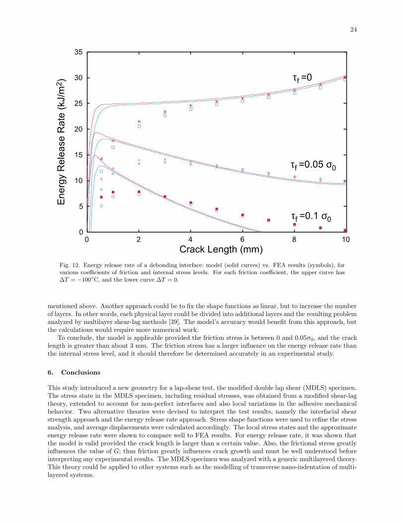
Figure 12 plots the energy release rate G calculated from the model (solid curves) compared to that obtainedby FEA (symbols), with and without internal stresses, and for various friction stresses. The calculationsshown were obtained for a fixed value of σ0 = 50 MPa. For a friction stress of τf = 0, the energy release rateincreases rapidly to about 25 kJ/m2 and then continues to increase, albeit slowly, to 30 kJ/m2. Because Gincreases with crack length, the prediction is that crack growth, once started, will be unstable until the endof the specimen. The situation changes dramatically when friction is added. When τf is not zero, the energyrelease rate rises to maximum for a certain crack length, and then decreases. In experiments, the predictionis that the crack will rapidly propagate to a length corresponding to the maximum G. Thereafter, becauseG decreases with crack length, the load will have to be increased to propagate the crack. In other words,friction stabilizes the crack propagation.

The shear-lag calculations agree very well with FEA at long crack length (a > 3 mm), but agree lesswell at shorter crack length. In particular, the maximum in G when there is friction, is at a much shortercrack length in the shear-lag analysis than in the FEA analysis. The shear-lag analysis was derived from ashear-lag stress analysis that ignores all singularities in the stress state. The energy release rate was derivedfrom a derivative of this stresses in this analysis. Such a derivative analysis will be accurate whenever theeffects of the singularity are small or whenever the contribution of the singularities is a constant. When theeffect is a constant, it will drop out in the differentiation step. Based on the results in Fig. 12 we claim thatthe singular effects at the crack tip are a constant provided the crack tip is not too close to the start of thespecimen. In other words, the shear-lag analysis is accurate provided a is not too short. When a is too short,the crack tip complexities will be influenced by the free surface. The shear-lag analysis does not accountfor this effect and thus the accuracy is lowered. Similar conclusions were reached in the analysis of debondgrowth and the fiber-matrix interface in the microbond specimen where a shear-lag analysis was shown toagree with FEA results provided the debond crack tip was not to close to either end of the specimen [44].

The effect of internal stresses, represented by the difference between the upper and lower curves obtainedfor a same friction stress but different ∆T , agrees very well with FEA calculations. This agreement follows

because the approximation of average axial stresses by shear lag is very accurate, and because σ(1)yy and σ

(3)yy

dominate the internal stress response of the system at long crack length. The accurate description of internalstress effects works for all values of friction stress.

The model accuracy is influenced by the choice of shape functions, and it is possible to improve theresults by adjusting them. Unfortunately, this approach only provides a partial solution to any disagreements

24

0

5

10

15

20

25

30

35

0 2 4 6 8 10

E

n

e

rg

y R

e

le

a

se

R

a

te

(kJ/m

2

)

Crack Length (mm)

τf =0

τf =0.05 σ

0

τf =0.1 σ

0

Fig. 12. Energy release rate of a debonding interface: model (solid curves) vs. FEA results (symbols), forvarious coefficients of friction and internal stress levels. For each friction coefficient, the upper curve has∆T = −100◦C, and the lower curve ∆T = 0.

mentioned above. Another approach could be to fix the shape functions as linear, but to increase the numberof layers. In other words, each physical layer could be divided into additional layers and the resulting problemanalyzed by multilayer shear-lag methods [39]. The model’s accuracy would benefit from this approach, butthe calculations would require more numerical work.

To conclude, the model is applicable provided the friction stress is between 0 and 0.05σ0, and the cracklength is greater than about 3 mm. The friction stress has a larger influence on the energy release rate thanthe internal stress level, and it should therefore be determined accurately in an experimental study.

6. Conclusions

This study introduced a new geometry for a lap-shear test, the modified double lap shear (MDLS) specimen.The stress state in the MDLS specimen, including residual stresses, was obtained from a modified shear-lagtheory, extended to account for non-perfect interfaces and also local variations in the adhesive mechanicalbehavior. Two alternative theories were devised to interpret the test results, namely the interfacial shearstrength approach and the energy release rate approach. Stress shape functions were used to refine the stressanalysis, and average displacements were calculated accordingly. The local stress states and the approximateenergy release rate were shown to compare well to FEA results. For energy release rate, it was shown thatthe model is valid provided the crack length is larger than a certain value. Also, the frictional stress greatlyinfluences the value of G; thus friction greatly influences crack growth and must be well understood beforeinterpreting any experimental results. The MDLS specimen was analyzed with a generic multilayered theory.This theory could be applied to other systems such as the modelling of transverse nano-indentation of multi-layered systems.


7. Acknowledgements

The authors are indebted to the Swiss National Science Foundation for financial support. One author (J.A. Nairn) was supported by a grant from the Mechanics of Materials program at the National ScienceFoundation (CMS-9713356).

REFERENCES

1. L.J. Hart-Smith. Bonded-bolted composite joints. In AIAA/ASME/ASCE/AHS 25th Structures, Struc-tural Dynamics and Materials Conference, pages 1–11, Palm Springs, California, May 14-16 1984. ASTM.

2. L.J. Hart-Smith. Design and analysis of bolted and riveted joints in fibrous composite structures. InInternational Symposium on Joining and Repair of Fibre-Reinforced Plastics, pages 1–15, London, Sept.10-11 1986. Imperial College.

3. Stress Analysis DE-Vol. 100, Reliability, Failure Prevention Aspects of Adhesive, Rubber ComponentsBolted Joints, and Composite Springs, editors. Stress Analysis And Strength Evaluation of Single-LapBand Adhesive Joints Subjected to External Bending Moments. ASME, ASME, 1998.

4. A.N. Gent and E.A. Meinecke. Compression, bending, and shear of bonded rubber blocks. Polym. Engin.Sci., 10:48–53, 1970.

5. A.N. Gent. Fracture mechanics of adhesive bonds. In The Rubber Division, pages 202–212, Denver,Colorado, Oct. 9-12 1973. Am. Chem. Soc.

6. S. Mall and K.M. Liechti, editors. On Three Dimensional Stress States in Adhesive Joints, Chicago,Illinois, Nov. 17- Dec. 2 1988. The American Society of Mechanical Engineers, The Winter AnnualMeeting of the American Society of Mechanical Engineers.

7. S.R. Pagano and N.J. Soni. Models for Studying Free-Edge Effects, volume 5 of Composite MaterialsSeries, R.B. Pipes Ed., chapter 1, pages 1–68. Elsevier Science Publishers, 1989.

8. ASTM D 1002-94. Standard Test Method for Apparent Shear Strength of Single-Lap-Joint AdhesivelyBonded Metal Specimens by Tension Loading, 1994.

9. ASTM D 3528 96. Standard Test Method for Strength Properties of Double Lap Shear Adhesive Jointsby Tension Loading, 1996.

10. O. Volkersen. Die nietkraftverteilung in zugbeanspruchten nietverbindungen mit konstanten laschen-querschnitten. Luftfahrtforschung, 15:41–47, 1938.

11. M. Goland and E. Reissner. The stresses in cemented joints. J. Appl. Mech., 11:A17–A27, 1944.

12. B. Broughton and M. Gower. Preparation and Testing of Adhesive Joints. Measurement Good PracticeGuide 47, National Physical Laboratory, Teddington, Middlesex, United Kingdom, TW11 0LW, 2001.

13. H. Chai and M.Y.M. Chiang. A crack propagation criterion based on local shear strain in adhesive bondssubjected to shear. J. Mech. Phys. Solids, 44:1669–1689, 1996.

14. G.P. Anderson and K.L. Devries. Analysis of Standard Bond-Strength Tests, volume 6, chapter 3, pages55–121. Marcel Dekker, Inc., New York and Basel, 1989.

15. P.R. Borgmeier and K.L. Devries. A fracture mechanics analysis of the effects of tapering adherends onthe strength of adhesive lap joints. J. Adhesion Sci. Technol., 7(9):967–986, 1993.

16. J.A. Nairn. Exact and variational theorems for fracture mechanics of composites with residual stresses,traction-loaded cracks, and imperfect interfaces. Int. J. Fract., 105:243–271, 2000.

17. F. Erdogan, F. Delale, and M.N. Aydinoglu. Stresses in adhesively bonded joints: A closed-form solution.J. Compos. Mater., 15:249–271, 1981.

18. W.C. Carpenter. A comparison of numerous lap joint theories for adhesively bonded joints. J. Adhesion,35:55–73, 1991.

19. M.Y.M. Chiang and H. Chai. Plastic deformation analysis of cracked adhesive bonds loaded in shear.Int. J. Solids Structures, 31:2477–2490, 1994.

20. M.Y.M. Chiang and H. Chai. A finite element analysis of interfacial crack propagation based on localshear, part I - near tip deformation. Int. J. Solids Structures, 00:14, 1997.

21. H. Chai and M.Y.M. Chiang. Finite element analysis of interfacial crack propagation based on localshear, part II - fracture. Int. J. Solids Structures, 00:14, 1997.

26

22. D.B. Bogy. Edge-bonded dissimilar orthogonal elastic wedges under normal and shear loading. J. Appl.Mech., (Sept.):460–466, 1968.

23. J. Dundurs. Edge-bonded dissimilar orthogonal elastic wedges under normal and shear loading. J. Appl.Mech., (September):650–652, 1969.

24. A. Gilibert and Y. Rigolot. Analyse asymptotique des assemblages colles a double recouvrement sollicitesau cisaillement en traction. Journal de Mecanique appliquee, 3:341–372, 1979.

25. K.L. DeVries and P.R. Borgmeier. Fracture mechanics analyses of the behavior of adhesion test specimens.VSP, 1998.

26. D.-A. Mendels, Y. Leterrier, and J.-A. E. Manson. The influence of internal stresses on the microbondtest 1: Theoretical analysis. J. Compos. Mater., in press, 2001.

27. D.-A. Mendels, Y. Leterrier, and J.-A. E Manson. The influence of internal stresses on the microbondtest 2: Experimental interpretation including the effect of relaxation. J. Compos. Mater., Accepted,2001.

28. L.J. Hart-Smith. Effects of flaws and porosity on strength of adhesive-bonded joints. Technical Re-port F33615-80-C-5092, PR No. 5, Douglas Aircraft Company, 3855 Lakewood Boulevard, Long Beach,California 90846, 1981.

29. M.L.L. Gilibert, Y. Klein, and A. Rigolot. Modelisation d’un composite plan en presence de micro-defauts. Technical Report 207, ENSTA, 1986.

30. L.J. Hart-Smith. Adhesive layer thickness and porosity criteria for bonded joints. Technical ReportF33615-80-C-5092, PR No. 3, Douglas Aircraft Company, 3855 Lakewood Boulevard, Long Beach, Cal-ifornia 90846, 1981.

31. D.-A. Mendels, J. Wolfrath, S.A. Page, J.-A. E. Manson, and C. Galiotis. A modified double lap-sheartest: Part 2, determination of local stress state by means of raman spectroscopy. Int. J. Adh. Adhes., tobe Submitted, 2000.

32. S.A. Page, D.-A. Mendels, L. Boogh, and J.-A.E. Manson. A modified double lap-shear test: Part 3, theinfluence of internal stresses on practical adhesion. Int. J. Adh. Adhes., to be Submitted, 2001.

33. D.-A. Mendels, Y. Leterrier, and J.-A.E. Manson. A modified double lap-shear test: Part 4, the influenceof physical aging on practical adhesion. Int. J. Adh. Adhes., to be Submitted, 2001.

34. D.-A. Mendels. A modified double lap shear test: Part 5, interfacial crack propagation in cross-plylaminates subjected to static or cyclic loading. Int. J. Adh. Adhes., to be Submitted, 2001.

35. S.A. Page, D.-A. Mendels, L. Boogh, and J.-A.E. Manson. Influence of the internal stress state on theadhesive performance of epoxy films determined by a new bonded-joint test. Brighton, UK, June 4-72000. IOM Publ. ltd.

36. S.A. Page, L. Boogh, and J.-A.E. Manson. Process and material tailoring for internal stress control. J.Appl. Polym. Sci., submitted, 2000.

37. D.-A. Mendels, Y. Leterrier, and J.-A.E. Manson. A stress transfer model for single fibre and plateletcomposites. J. Compos. Mater., 33:1525–1544, 1999.

38. D.-A. Mendels, Y. Leterrier, and J.-A.E. Manson. Property modelling of epoxy laminates including ther-mal stresses and relaxation behaviour upon physical aging. In A.H. Cardon, editor, DURACOSYS’99,Brussels, July 12-14 1999. Balkema.

39. J.A. Nairn and D.-A. Mendels. On the use of planar shear-lag methods for stress-transfer analysis ofmultilayered composites. Mech. Mater., 33:335–362, 2001.

40. D.-A. Mendels, S.A. Page, Y. Leterrier, and J.-A.E. Manson. A modified double lap-shear test as a meanto measure intrinsic properties of adhesive joints. Brighton, UK, June 4-7 2000. IOM Publ. ltd.

41. D.-A. Mendels. Analysis of the single-fibre fragmentation test. NPL Report MATC (A)17, NationalPhysical Laboratory, Teddington, Middlesex, United Kingdom, TW11 0LW, 2001.

42. M.J. Lodeiro, S. Maugdal, L.N. McCartney, R. Morrell, and B. Roebuck. Critical review of interfacemethods for composites. NPL Report CMMT(A)101, National Physical Laboratory, 1998.

43. L.N. McCartney. Stress transfer mechanics for systems of transverse isotropic concentric cylinders, I-basic theory. in preparation, 2001.

44. C.H. Liu and J.A. Nairn. Analytical Fracture Mechanics of the Microbond Test Including the Effects ofFriction and Thermal Stresses. J. of Adhes. and Adhesives, 19:59–70, 1999.

a compression-loaded double lap shear test: part 1, … · international journal of adhesion and...

Documents