a comprehensive trainable error model for sung music queries

Journal of Artificial Intelligence Research 22 (2004) 57-91 Submitted 07/03; published 08/04

A Comprehensive Trainable Error Model for Sung Music

Queries

Colin J. Meek [email protected]

Microsoft Corporation, SQL Server,

Building 35/2165, 1 Microsoft Way, Redmond WA 98052 USA

William P. Birmingham [email protected]

Grove City College, Math and Computer Science,

Faculty Box 2655, 100 Campus Drive, Grove City PA 16127 USA

Abstract

We propose a model for errors in sung queries, a variant of the hidden Markov model(HMM). This is a solution to the problem of identifying the degree of similarity betweena (typically error-laden) sung query and a potential target in a database of musical works,an important problem in the field of music information retrieval. Similarity metrics area critical component of “query-by-humming” (QBH) applications which search audio andmultimedia databases for strong matches to oral queries. Our model comprehensivelyexpresses the types of error or variation between target and query: cumulative and non-cumulative local errors, transposition, tempo and tempo changes, insertions, deletions andmodulation. The model is not only expressive, but automatically trainable, or able to learnand generalize from query examples. We present results of simulations, designed to assessthe discriminatory potential of the model, and tests with real sung queries, to demonstraterelevance to real-world applications.

1. Introduction

Many approaches have been proposed for the identification of viable targets for a query ina music database. Query-by-humming systems attempt to address the needs of the non-expert user, for whom a natural query format – for the purposes of finding a tune, hookor melody of unknown providence – is to sing it. Our goal is to demonstrate a unifyingmodel, expressive enough to account for the complete range of modifications observed in theperformance and transcription of sung musical queries. Given a complete model for singererror, we can accurately determine the likelihood that, given a particular target (or song ina database), the singer would produce some query. These likelihoods offer a useful measureof similarity, allowing a query-by-humming (QBH) system to identify strong matches toreturn to the user.

Given the rate at which new musical works are recorded, and given the size of multimediadatabases currently deployed, it is generally not feasible to learn a separate model for eachtarget in a multimedia database. Similarly, it may not be possible to customize an errormodel for every individual user. As such, a QBH matcher must perform robustly across abroad range of songs and singers. We develop a method for training our error model thatfunctions well across singers with a broad range of abilities, and successfully generalizesto works for which no training examples have been given (see Section 11). Our approach(described in Section 9) is an extension of a standard re-estimation algorithm (Baum &

c©2004 AI Access Foundation. All rights reserved.

Meek & Birmingham

Eagon, 1970), and a special case of Expectation Maximization (EM) (Dempster, Laird, &Jain, 1977). It is applicable to hidden Markov models (HMM) with the same dependencystructure, and is demonstrated to be convergent (see Appendix A).

2. Problem Formulation and Notation

An assumption of our work is that pitch and IOI adequately represent both the target andthe query. This limits our approach to monophonic lines, or sequences of non-overlappingnote events. An event consists of a 〈Pitch, IOI〉 duple. IOI is the time difference betweenthe onsets of successive notes, and pitch is the MIDI note number1.

We take as input a note-level abstraction of music. Other systems act on lower-levelrepresentations of the query. For instance, a frame-based frequency representation is oftenused (Durey, 2001; Mazzoni, 2001). Various methods for the translation of frequency andamplitude data into note abstraction exist (Pollastri, 2001; Shifrin, Pardo, Meek, & Birm-ingham, 2002). Our group currently uses a transcriber based on the Praat pitch-tracker(Boersma, 1993), designed to analyze voice pitch contour. A sample Praat analysis is shownin Figure 1. In addition to pitch extraction, the query needs to be segmented, or organizedinto contiguous events (notes). The query transcription process is described in greater de-tail in Section 3. Note that these processes are not perfect, and it is likely that error willbe introduced in the transcription of the query.

42

44

46

48

50

52

Time (sec.)

Pitc

h (

60 =

Mid

dle

C)

0 0.2 0.4 0.6 0.8 1 1.2 1.40.5

0.6

0.7

0.8

0.9

1

Auto

corr

ela

tion v

alu

e

0 0.2 0.4 0.6 0.8 1 1.2 1.4-0.1

-0.05

0

0.05

0.1

Am

plit

ude

Original (transposed) Query

join + local error

Time (sec.)

Figure 1: Sample query transcription: from Hey Jude by the Beatles, the word “better”

Restricting ourselves to this event description of target and query ignores several ele-ments of musical style, including dynamics, articulation and timbre, among others. Objec-tively and consistently characterizing these features is quite difficult, and as such we havelittle confidence they can be usefully exploited for music retrieval at this point. We acknowl-edge, however, the importance of such elements in music query/retrieval systems in general.They will likely prove essential in refining or filtering the search space (Birmingham, Pardo,

1. Musical Instrument Digital Interface (MIDI) has become a standard electronic transmission and storageprotocol/format for music. MIDI note numbers essentially correspond to the keys of a piano, where’middle C’ corresponds to the integer value 60.

58

A Comprehensive Trainable Error Model for Sung Music Queries

Meek, & Shifrin, 2002; Birmingham, Dannenberg, Wakefield, Bartsch, Bykowski, Mazzoni,Meek, Mellody, & Rand, 2001).

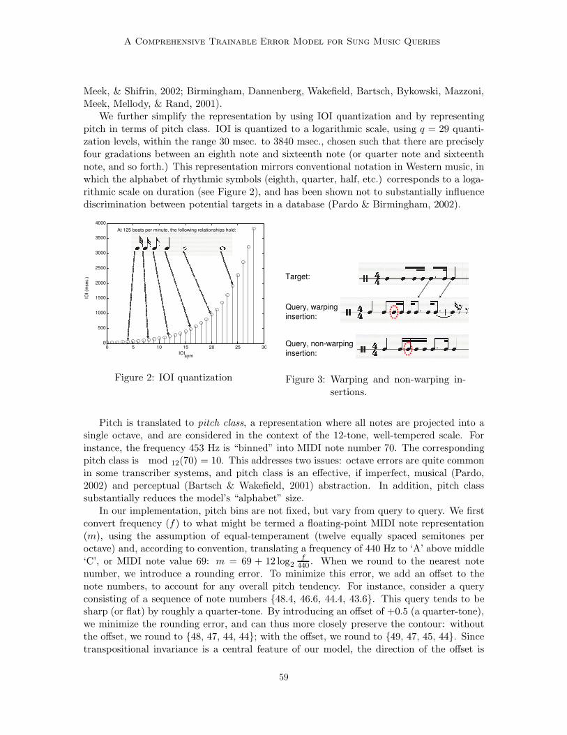
We further simplify the representation by using IOI quantization and by representingpitch in terms of pitch class. IOI is quantized to a logarithmic scale, using q = 29 quanti-zation levels, within the range 30 msec. to 3840 msec., chosen such that there are preciselyfour gradations between an eighth note and sixteenth note (or quarter note and sixteenthnote, and so forth.) This representation mirrors conventional notation in Western music, inwhich the alphabet of rhythmic symbols (eighth, quarter, half, etc.) corresponds to a loga-rithmic scale on duration (see Figure 2), and has been shown not to substantially influencediscrimination between potential targets in a database (Pardo & Birmingham, 2002).

0 5 10 15 20 25 300

500

1000

1500

2000

2500

3000

3500

4000

IOI (m

sec.)

IOIsym

At 125 beats per minute, the following relationships hold:

Figure 2: IOI quantization

Target:

Query, warpinginsertion:

Query, non-warping

insertion:

Figure 3: Warping and non-warping in-sertions.

Pitch is translated to pitch class, a representation where all notes are projected into asingle octave, and are considered in the context of the 12-tone, well-tempered scale. Forinstance, the frequency 453 Hz is “binned” into MIDI note number 70. The correspondingpitch class is mod 12(70) = 10. This addresses two issues: octave errors are quite commonin some transcriber systems, and pitch class is an effective, if imperfect, musical (Pardo,2002) and perceptual (Bartsch & Wakefield, 2001) abstraction. In addition, pitch classsubstantially reduces the model’s “alphabet” size.

In our implementation, pitch bins are not fixed, but vary from query to query. We firstconvert frequency (f) to what might be termed a floating-point MIDI note representation(m), using the assumption of equal-temperament (twelve equally spaced semitones peroctave) and, according to convention, translating a frequency of 440 Hz to ‘A’ above middle‘C’, or MIDI note value 69: m = 69 + 12 log2

f440 . When we round to the nearest note

number, we introduce a rounding error. To minimize this error, we add an offset to thenote numbers, to account for any overall pitch tendency. For instance, consider a queryconsisting of a sequence of note numbers {48.4, 46.6, 44.4, 43.6}. This query tends to besharp (or flat) by roughly a quarter-tone. By introducing an offset of +0.5 (a quarter-tone),we minimize the rounding error, and can thus more closely preserve the contour: withoutthe offset, we round to {48, 47, 44, 44}; with the offset, we round to {49, 47, 45, 44}. Sincetranspositional invariance is a central feature of our model, the direction of the offset is

59

Meek & Birmingham

irrelevant in this example. Adopting an approach proposed for a QBH “audio front end”(Pollastri, 2001), we consider several offsets (O = {0.0, 0.1, . . . , 0.9}). Given a sequenceof note numbers (M = {m1, m2, . . . , mn}), we choose the offset (o ∈ O) such that the

mean error squared (e =�n

i=1[m+o−round(m+o)]2

n) is minimized, and set Pitch[i] equal to

round(mi + o).We choose discrete sets of symbols to represent pitch and duration since, as will be seen,

a continuous representation would necessitate an unbounded number of states in our model.This second event representation is notated:

ot = 〈P [t], R[t]〉 (1)

for queries (using the mnemonic shorthand observation = 〈Pitch,Rhythm〉). Target eventsare similarly notated:

di = 〈P [i], R[i]〉 (2)

For clarity, we will return to the earlier representation 〈Pitch[i], IOI[i]〉 where appropriate.The second representation is derived from the first as follows, where 30 and 3840 are theIOI values associated with the centers of the shortest and longest bins, and q is the numberof IOI quantization bins:

P [i] = mod 12(Pitch[i]) (3)

R[i] = round

(log IOI[i] − log 30

log 3840 − log 30· (q − 1)

)

(4)

The goal of this paper is to present a model for query errors within the scope of this simpleevent representation. We will first outline the relevant error classes, and then present anextended Hidden Markov Model accounting for these errors. Taking advantage of certainassumptions about the data, we can then efficiently calculate the likelihood of a targetmodel generating a query. This provides a means of ranking potential targets in a database(denoted {D1,D2, . . .}, where Di = {d1, d2, . . .}) given a query (denoted O = {o1, o2, . . .})based on the likelihood the models derived from those targets generated a given query. Asummary of the notation used in this paper is provided in Appendix B.

3. Query Transcription

Translating from an audio query to a sequence of note events is a non-trivial problem. Wenow outline the two primary steps in this translation: frequency analysis and segmentation.

3.1 Frequency Analysis

We use the Praat pitch-tracker (Boersma, 1993), an enhanced auto-correlation algorithm de-veloped for speech analysis, for this stage. This algorithm identifies multiple auto-correlationpeaks for each analysis frame, and chooses a path through these peaks that avoids pitchjumps and favors high correlation peaks. For a particular frame, no peak need be chosen,resulting in gaps in the frequency analysis. In addition, the algorithm returns the auto-correlation value at the chosen peak (which we use as a measure of pitch-tracker confidence),and the RMS amplitude by frame (see Figure 1 for instance.)

60


3.2 Segmentation

A binary classifier is used to decide whether or not each analysis frame contains the begin-ning of a new note. The features considered by the classifier are derived from the pitch-tracker output. This component is currently in development at the University of Michigan.In its present implementation, a five-input, single-layer neural network performs the clas-sification. We assign a single pitch to each note segment, based on the weighted averagepitch by confidence of the frames contained in the segment. An alternative implementationis currently being explored, which treats the query analysis as a signal (ideal query) withnoise, and attempts to uncover the underlying signal using Kalman-filter techniques.

4. Error Classes

A query model should be capable of expressing the following musical – or un-musical youmight argue – transformations, relative to a target:

1. Insertions and deletions: adding or removing notes from the target, respectively.These edits are frequently introduced by transcription tools as well.

2. Transposition: the query may be sung in a different key or register than the target.Essentially, the query might sound “higher” or “lower” than the target.

3. Tempo: the query may be slower or faster than the target.

4. Modulation: over the course of a query, the transposition may change.

5. Tempo change: the singer may speed up or slow down during a query.

6. Non-cumulative local error: the singer might sing a note off-pitch or with poor rhythm.

4.1 Edit Errors

Insertions and deletions in music tend to influence surrounding events. For instance, whenan insertion is made, the inserted event and its neighbor tend to occupy the temporal spaceof the original note: if an insertion is made and the duration of the neighbors is not modified,the underlying rhythmic structure (the beat) is changed. We denote this type of insertion a“warping” insertion. For instance, notice the alignment of notes after the warping insertionin Figure 3, indicated by the dotted arrows. The inserted notes are circled. For the non-warping insertion, the length of the second note is shortened to accommodate the newnote.

With respect to pitch, insertions and deletions do not generally influence the surroundingevents. However, previous work assumes this kind of influence: noting that intervalliccontour tends to be the strongest component in our memory of pitch; one researcher hasproposed that insertions and deletions could in some cases have a “modulating” effect(Lemstrom, 2000), where the edit introduces a pitch offset, so that pitch intervals ratherthan the pitches themselves are maintained. We argue that relative pitch, with respect tothe query as a whole, should be preserved. Consider the examples in Figure 4. The firstrow of numbers below the staff indicates MIDI note numbers, the second row indicates the

61

Meek & Birmingham

intervals in semitones (‘u’ = up, ‘d’ = down.) Notice that the intervallic representation ispreserved in the modulating insertion, while the overall “profile” (and key) of the line ismaintained in the non-modulating insertion.

Target:

Query, modulating

insertion:

Query,

non-modulating

insertion:

Figure 4: Modulating and non-modulating insertions

time

pitch

time

pitch

INSERTION

IOIa

IOIb

IOIc

IOId

IOIinsert

Pitcha

Pitchb

Pitchd

Pitchc

Pitchinsert

Figure 5: Insertion of a note event in aquery

The effects of these various kinds of insertions and deletions are now formalized, withrespect to a target consisting of two events {〈Pitcha, IOIa〉, 〈Pitchb, IOIb〉}, and a query{〈Pitchc, IOIc〉, 〈PitchinsertIOIinsert〉〈Pitchd, IOId〉}, where 〈PitchinsertIOIinsert〉 is theinserted event (see Figure 5). Note that deletion is simply the symmetric operation, so weshow examples of insertions only:

• Effects of a warping insertion on IOI: IOIc = IOIa, IOId = IOIb

• Effects of a non-warping insertion on IOI: IOIc = IOIa − IOIinsert, IOId = IOIb

• Effects of a modulating insertion on pitch: Pitchc = Pitcha, Pitchd = Pitchinsert +Pitchb − Pitcha︸︷︷︸

pitch contour

• Effects of a non-modulating insertion on pitch: Pitchc = Pitcha, Pitchd = Pitchb

In our model, we deal only with non-modulating and non-warping insertions and dele-tions explicitly, based on the straightforward musical intuition that insertions and deletionstend to operate within a rhythmic and modal context. The other types of edit are rep-resented in combination with other error classes. For instance, a modulating insertion issimply an insertion combined with a modulation.

Another motivation for our “musical” definition of edit is transcriber error. In thiscontext, we clearly would not expect the onset times or pitches of surrounding events to beinfluenced by a “false hit” insertion or a missed note. The relationships amongst successiveevents must therefore be modified to avoid warping and modulation. Reflecting this bias,we use the terms “join” and “elaboration” to refer to deletions and insertions, respectively.A system recognizing musical variation (Mongeau & Sankoff, 1990) uses a similar notion ofinsertion and deletion, described as “fragmentation” and “consolidation” respectively.

62


4.2 Transposition and Tempo

We account for the phenomenon of persons reproducing the same “tune” at different speedsand in different registers or keys. Few people have the ability to remember and reproduceexact pitches (Terhardt & Ward, 1982), an ability known as “absolute” or “perfect” pitch.As such, transpositional invariance is a desirable feature of any query/retrieval model. Theeffect of transposition is simply to add a certain value to all pitches. Consider for examplethe transposition illustrated in Figure 6, Section a, of Trans = +4.

time

pitch

Scale= 1.5

Trans=+4

query

target

overlap

time

pitch

Change=1.5

Modu=+ 2

time

pitch

RError=1.5

PError=-1

a)

b) c)

Figure 6: Error class examples, openingnotes of Brahms’ Cello Sonatain e-minor

0 1 2 3 4 5 6 7 80

0.1

0.2

0.3

0.4

0.5

0.6

0.7

0.8

0.9

1

Time (sec.)

Ra

tio

of

Cu

rre

nt

Lo

ca

l T

em

po

to

Ma

xim

um

Figure 7: Tempo increase

Tempo in this context is simply the translation of rhythm, which describes durationrelationships, into actual time durations. Again, it is difficult to remember and reproducean exact tempo. Moreover, it is very unlikely that two persons would choose the samemetronome marking, much less unconstrained beat timing, for any piece of music. This is anatural “musical” interpretation. We measure tempo relative to the original using a scalingfactor on rhythmic duration. Thus, if the query is 50% slower than the target, we have ascaling value of Scale = 1.5, as shown in Figure 6, Section a.

In practice, we use quantized tempo scaling and duration values. Note that additionin the logarithmic scale is equivalent to multiplication: with quantized IOI values, wereplace floating point multiplication with integer addition when applying a scaling value.For instance, given our quantization bins, a doubling of tempo always corresponds to anaddition of four: Scale = 2.0 ↔ Scalequantized = +4.

4.3 Modulation and Tempo Change

Throughout a query, the degree of transposition or tempo scaling can change, referred to asmodulation and tempo change, respectively. Consider a query beginning with the identitytransposition Trans = 0 and identity tempo scaling Scale = 1, as in Figure 6, Section b.When a modulation or tempo change is introduced, it is always with respect to the previoustransposition and tempo. For instance, on the third note of the example, a modulation ofModu = +2 occurs. For the remainder of the query, the transposition is equal to 0+2 = +2,

63

Meek & Birmingham

from the starting reference transposition of 0. Similarly, the tempo change of Change = 1.5on the second note means that all subsequent events occur with a rhythmic scaling of1 · 1.5 = 1.5.

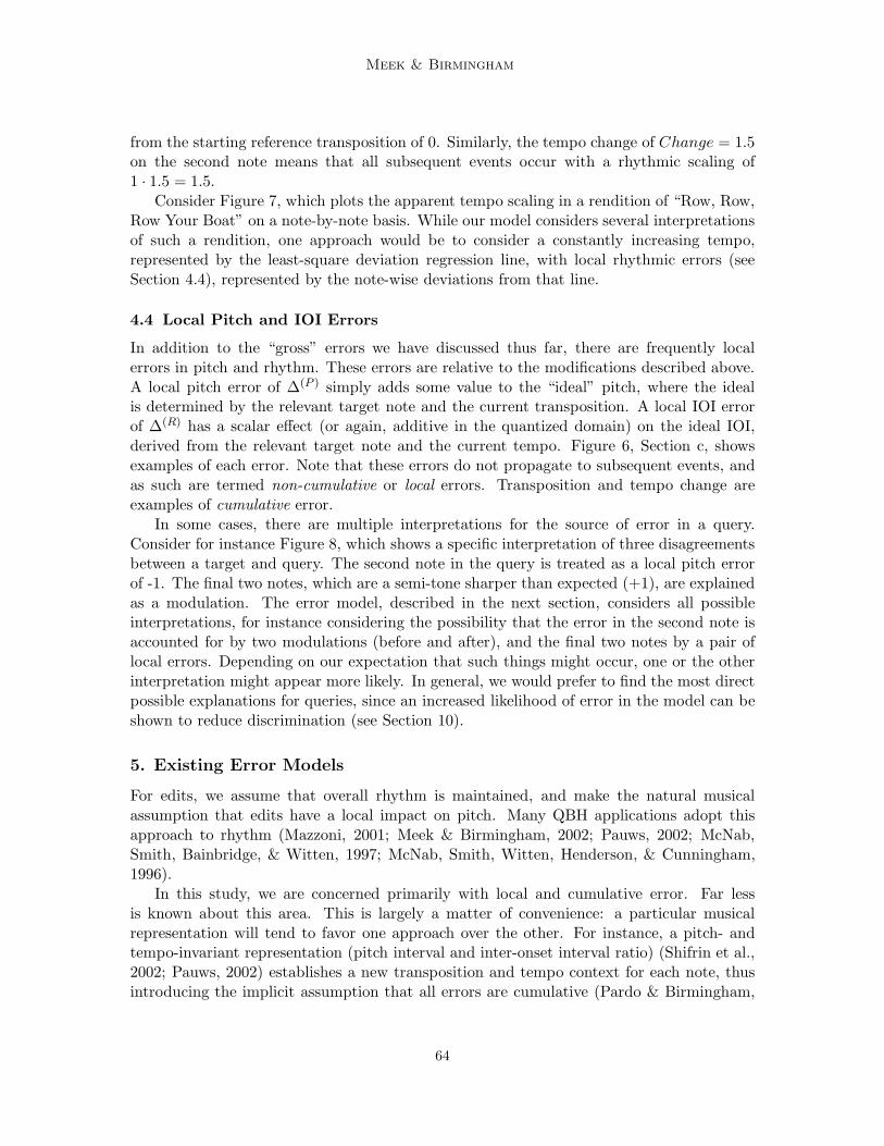
Consider Figure 7, which plots the apparent tempo scaling in a rendition of “Row, Row,Row Your Boat” on a note-by-note basis. While our model considers several interpretationsof such a rendition, one approach would be to consider a constantly increasing tempo,represented by the least-square deviation regression line, with local rhythmic errors (seeSection 4.4), represented by the note-wise deviations from that line.

4.4 Local Pitch and IOI Errors

In addition to the “gross” errors we have discussed thus far, there are frequently localerrors in pitch and rhythm. These errors are relative to the modifications described above.A local pitch error of ∆(P ) simply adds some value to the “ideal” pitch, where the idealis determined by the relevant target note and the current transposition. A local IOI errorof ∆(R) has a scalar effect (or again, additive in the quantized domain) on the ideal IOI,derived from the relevant target note and the current tempo. Figure 6, Section c, showsexamples of each error. Note that these errors do not propagate to subsequent events, andas such are termed non-cumulative or local errors. Transposition and tempo change areexamples of cumulative error.

In some cases, there are multiple interpretations for the source of error in a query.Consider for instance Figure 8, which shows a specific interpretation of three disagreementsbetween a target and query. The second note in the query is treated as a local pitch errorof -1. The final two notes, which are a semi-tone sharper than expected (+1), are explainedas a modulation. The error model, described in the next section, considers all possibleinterpretations, for instance considering the possibility that the error in the second note isaccounted for by two modulations (before and after), and the final two notes by a pair oflocal errors. Depending on our expectation that such things might occur, one or the otherinterpretation might appear more likely. In general, we would prefer to find the most directpossible explanations for queries, since an increased likelihood of error in the model can beshown to reduce discrimination (see Section 10).

5. Existing Error Models

For edits, we assume that overall rhythm is maintained, and make the natural musicalassumption that edits have a local impact on pitch. Many QBH applications adopt thisapproach to rhythm (Mazzoni, 2001; Meek & Birmingham, 2002; Pauws, 2002; McNab,Smith, Bainbridge, & Witten, 1997; McNab, Smith, Witten, Henderson, & Cunningham,1996).

In this study, we are concerned primarily with local and cumulative error. Far lessis known about this area. This is largely a matter of convenience: a particular musicalrepresentation will tend to favor one approach over the other. For instance, a pitch- andtempo-invariant representation (pitch interval and inter-onset interval ratio) (Shifrin et al.,2002; Pauws, 2002) establishes a new transposition and tempo context for each note, thusintroducing the implicit assumption that all errors are cumulative (Pardo & Birmingham,

64


2002). A study of sung queries (Pollastri, 2001) determined that cumulative error is in factfar less common than local error, a conclusion supported by our studies.

Another approach to the differences in transposition and tempo context is to attemptmultiple passes over a fixed context model, and evaluate error rigidly within each passby comparing the query to various permutations of the target. Dynamic time-warpingapproaches (Mazzoni, 2001) and non-distributed HMM techniques (Durey, 2001) are well-suited to this technique. It is not possible to model, for instance, a modulation, using thesemethods, only local error. A preliminary QBH proposal (Wiggins, Lemstrom, & Meredith,2002) recommends a similar approach, grouping together “transposition vectors” connectingquery and target notes. Such approaches are amenable to extensions supporting cumulativeerror as well, but have not – to our knowledge – been extended in this way.

An alternative is to normalize the tempo of the query by either automated beat-tracking,a difficult problem for short queries, or, more effectively, by giving the querier an audiblebeat to sing along with – a simple enough requirement for users with some musical back-ground (Chai, 2001). Again, there is an assumption that the transposition will not changeduring a query, but the beat-tracker can adapt to changing tempi.

5.1 Alternative Approaches

We are concerned primarily with sequence based approaches to music retrieval. It is possibleto relax this assumption somewhat, by translating targets into Markov models where thestate is simply a characteristic relationship between consecutive notes, allowing for loopsin the model (Shifrin et al., 2002). Borrowing from the text search world, we can alsomodel music as a collection of note n-grams, and apply standard text retrieval algorithms(Downie, 1999; Tseng, 1999). In query-by-humming systems, the user is searching for asong that “sounds like...” rather than a song that is “about” some short snippet of notes,if it makes sense to discuss music in these terms at all2. For this reason, we believe thatsequence-based methods can more accurately represent music in this context.

Original (transposed)

Query

modulation

local pitch error

Figure 8: Portion of a query on theAmerican National Anthem,including examples of modula-tion and local pitch error

a b

0.1

0.1 0.90.9

1 2 3 4 5 60

0.05

0.1

0.15

0.2

Roll Result

Pro

ba

bili

ty

1 2 3 4 5 60

0.1

0.2

0.3

0.4

0.5

Roll Result

Pro

ba

bili

ty

Figure 9: Simple HMM, the dishonestgambler

2. Beethoven’s Fifth Symphony is a notable exception

65

Meek & Birmingham

5.2 Indexing and Optimization Techniques

It should be noted that as a general model, JCS cannot take advantage of optimizationsspecific to certain specializations. For instance, the cumulative-only version is amenable to arelative note representation, a transposition- and tempo- invariant representation, obviatingthe need to compare a query with multiple permutations of the target.

Existing indexing techniques for string-edit distance metrics – for instance using suf-fix trees (Chavez & Navarro, 2002; Gusfield, 1997) and so-called ‘wavelet’ approximations(Kahveci & Singh, 2001) – are appropriate for k-distance searches, and thus might proveuseful as a pre-filtering mechanism. However, they are not readily adaptable to more sophis-ticated probabilistic matching metrics, and, more importantly, rely on a global alignmentassumption infeasible for QBH applications. A recent application of dynamic time-warpingindexing to music retrieval (Zhu & Shasha, 2003) relies on the assumption that the queryis globally aligned to the target, which is feasible only when the query covers precisely thematerial in the target.

Other indexing techniques can provide benefits even in the general case. Lexical treesare commonly used in speech recognition for large-vocabulary recognition (Huang, Acero,& Hon, 2001), and can be adapted to the alignment and metric requirements of JCS us-ing similar trie structures. Linear search using sub-optimal heuristics has been applied tosequence matching in bio-informatics (Pearson, 1998; Altschul, Madden, Schaffer, Zhang,Zhang, Miller, & Lipman, 1997). These approaches are fast for massive databases, and rea-sonably accurate even with low similarity distance metrics. Optimal alignment techniques– adaptable to arbitrary probabilistic sequence alignment models – are also being devel-oped using trie indices (Meek, Patel, & Kasetty, 2003) and parallel architectures (Shpaer,Robinson, Yee, Candlin, Mines, & Hunkapiller, 1996).

We are concerned primarily with determining appropriate metrics for QBH applications.Once this has been accomplished, it will be possible to choose and develop appropriateoptimizations and indexing techniques for large-scale deployment.

6. Hidden Markov Models

Hidden Markov Models (HMM) are the basis for our approach. We will begin by describinga simple HMM, and then describe the extensions to the model necessary for the currenttask. As suggested by the name, HMMs contain hidden, or unobserved, states. As a simpleexample, consider a dishonest gambler, who is known to occasionally swap a fair dice fora loaded dice (with thanks to “Biological Sequence Analysis” (Durbin, Eddy, Krogh, &G.Mitchison, 1998) for the example). Unfortunately, it is impossible to observe (directly)which of the dice is being used, since they are visually indistinguishable. For this reason,we define two hidden states, a and b, representing the conjectures that the gambler is usingfair and loaded dice, respectively. Further, we represent our expectation that the gamblerwill switch dice or stay with a dice using a transition diagram, where the transitions haveassociated probabilities (see Figure 9). For instance, the arc from a → b is labelled 0.1,indicating that the probability of the gambler switching from the fair dice to the loaded diceafter a roll is 0.1, or formally Pr(qt+1 = b|qt = a, λ) where qt is the current state at timeinterval t, and λ is the model. What we can directly observe in this example is the resultof each roll. While we do not know which dice is being used, we know some distribution

66


over the roll values for each dice (shown at the bottom of Figure 9). These are refereedto as observation or emission probability functions, since they describe the probability ofemitting a particular observation in a state.

In the music information-retrieval (MIR) context, we have a series of models, eachrepresenting a possible database target, and wish to determine which is most likely givena query, represented by a sequence of pitch and rhythm observations. To draw a parallelto our gambler example, we might want to determine whether we are dealing with thedishonest gambler described above, or an honest gambler (see Figure 10) who uses only fairdice. Given some sequence of observations, or dice rolls, we can determine the likelihoodthat each of the models generated that sequence.

a

1.0

1 2 3 4 5 6

0

0.05

0.1

0.15

0.2

Roll Result

Pro

babi

lity

Figure 10: Simple HMM, the honestgambler

s1 s2 s3

null null

Figure 11: A model with skips and nullstates

6.1 Honest or Dishonest? An example

The strength of the HMM approach is that it is straightforward to determine the likelihoodof any observation sequence if the transition probabilities and emission probabilities areknown. Conceptually, the idea is to consider all possible paths through the model consis-tent with the observation sequence (e.g., the observed dice rolls), and take the sum of theprobabilities of each path given those observations. For instance, the roll sequence {1, 5, 4}could be generated by one of four paths in the dishonest gambler model, assuming that thedishonest gambler always begins with the fair dice: {{a, a, a}, {a, a, b}, {a, b, a}, {a, b, b}}.The probability of the second path, for instance, is equal to the probability of the transitions(Pr(a → a) ·Pr(a → b)=0.9 · 0.1 = 0.09) multiplied by the probabilities of the observationsgiven the states in the path (the probability of rolling 1 then 5 with the fair dice, by theprobability of rolling 4 with the loaded dice: 0.167 · 0.167 · 0.5 = 0.0139), which is equalto 1.25e-3. To determine the likelihood of the observation sequence given the model, wesimply take the sum of the probabilities of each path (3.75e-3 + 1.25e-3 + 2.78e-5 + 7.50e-4= 5.78e-3.) The honest gambler is in effect a fully observable model, since there is onlya single hidden state. Only one path through this model is possible, and its likelihood istherefore a function of the observation probabilities only since the path is deterministic (1.0transition probabilities): (0.167)3 = 4.63e−3. From this, we can conclude that the sequence

67

Meek & Birmingham

of rolls 1, 5, 4 is more likely to have been generated by a dishonest gambler, though weshould note that three rolls do not provide much evidence one way or the other!

7. Extended HMM

In the context of our query error model, we account for edit errors (insertions and deletions)in the “hidden” portion of the model. Using the notion of state “clusters,” we account fortransposition, modulation, tempo and tempo changes. Fine pitch and rhythm errors areaccounted for in the observation distribution function.

7.1 State Definition

The state definition incorporates three elements: edit type (Edit), transposition (Key) andtempo (Speed). States are notated as follows:

sx = 〈E[x],K[x], S[x]〉, 1 ≤ x ≤ n (5)

If E is the set of all edit types, K is the set of all transpositions, and S is the set of alltempi, then the set of all states S is equal to:

E× K × S (6)

We now define each of these sets:

7.1.1 Edit Type

For the sake of notational clarity, we do not enumerate the edit types in E, but define themin terms of symbols that indirectly refer to events in the target sequence, encoding positioninformation. There are three types of symbol:

• Samei: refers to the correspondence between the ith note in the target and an eventin the query.

• Joinli: refers to a “join” of l notes, starting from the ith note in the target. In other

words, a single note in the query replaces l notes in the target.

• Elabmi,j : refers to the jth query note elaborating the ith target note. In other words, a

single note in the target is replaced by m notes in the query.

Notice that Samei = Join1i = Elab1

i,1, each referring to a one-to-one correspondence between

target and query notes. In our implementation, Join1i plays all three roles. We generate a

set of states for a given target consisting of, for each event in the target di:

• A Samei state.

• Join states Joinli, for 2 ≤ l ≤ L where L is some arbitrary limit on the number of

events that can be joined.

• Elaboration states Elabmi,j for 2 ≤ m ≤ M and 1 ≤ j ≤ m, where M is some arbitrary

limit on the length of elaborations.

68


Why do we have so many states to describe each event in the target? We wish to establisha one-to-one correspondence between hidden states and query events, to simplify the im-plementation, which is why we introduce multiple states for each elaboration. We choosenot to implement joins by “skips” through a reduced set of states, or elaborations as nullstates, since as discussed, edits influence our interpretation of the underlying target events.Figure 11 illustrates a model with skips and null states. Given our definition of insertionand deletion, state s1 would need separate emission probability tables for each outward arc(and thus would be functionally and computationally equivalent to the model we propose).

As mentioned, we explicitly handle only non-modulating and non-warping insertionsand deletions (see Section 4.1). As such, when comparing target and query events withrespect to a join, we generate a longer target note, with the sum duration of the relevanttarget events, and the pitch of the first. Similarly, for an elaboration, we treat a sequence ofquery notes as a single, longer event. Figure 12 shows a portion of the hidden state graphrelating a target and query through a sequence of hidden states, where the dotted notes areexamples of each generated note.

SameState:

Target:

Query:

Elab2

Join2

Elab2

2

Figure 12: Relationship between statesand events

States referencing the 1st target event.

elaboration =

junction (shorthand): =

Same1 Same2 Same3 Same4

Join12

Join22

Join32

Join42

Elab1,12

Elab2,12

Elab3,12

Elab4,12

Elab1,22

...

Figure 13: Edit type topology

Where 〈Pitch[i], IOI[i]〉 is the ith query note, and 〈Pitch[t], IOI[t]〉 the tth target note,we have the following expected relationships between target and query based on the hiddenstate at time t, qt = 〈E[t], 0, 0〉, ignoring transposition, tempo and local error for the

69

Meek & Birmingham

moment:

〈Pitch[i], IOI[i]〉 = 〈Pitch[t], IOI[t]〉, if E[t] = Samei

〈Pitch[i],∑i+l−1

j=i IOI[j]〉 = 〈Pitch[t], IOI[t]〉, if E[t] = Joinli

〈Pitch[i], IOI[i]〉 = 〈Pitch[t − j + 1],

t+m−j∑

k=t

IOI[k]〉

︸︷︷︸

Notice that all events in the elaboration point to a single larger event

if E[t] = Elabmi,j

(7)

7.1.2 Transposition and Tempo

In order to account for the various ways in which target and query could be related, we mustfurther refine our state definition to include transposition and tempo cluster. The intuitionhere is that the edit type determines the alignment of events between the query with thetarget (see Figure 12 for instance) and the cluster determines the exact relationship betweenthose events.

Using pitch class, there are only twelve possible distinct transpositions, because of themodulus-12 relationship to pitch. While any offset will do, we set K = {−5,−4, . . . ,+6}.We establish limits on how far off target a query can be with respect to tempo, allowing thequery to be between half- and double- speed. This corresponds to values in the range S ={−4,−3, . . . ,+4} in terms of quantized tempo units (based on the logarithmic quantizationscale described in Section B).

7.2 Transition Matrix

We now describe the transition matrix A, which maps from S × S → <. Where qt is thestate at time t (as defined by the position in the query, or observation sequence), axy isequal to the probability Pr(qt = sx|qt+1 = sy, λ), or in other words, the probability of atransition from state sx to state sy.

The transition probability is composed of three values, an edit type, modulation andtempo change probability:

axy = aExy · a

Kxy · a

Sxy (8)

We describe each of these values individually.

7.2.1 Edit Type Transition

Most of the edit type transitions have zero probability, as suggested by the state descriptions.For instance, Samei states can only precede states pointing to index i + 1 in the target.Elaboration states are even more restrictive, as they form deterministic chains of the form:Elabm

i,1 → Elabmi,2, → . . . → Elabm

i,m. This last state can then proceed like Samei, to the

i + 1 states. Similarly, Joinli states can only proceed to i + l states. A sample model

topology is shown in Figure 13, for M = L = 2. Note that this is a left-right model, inwhich transitions impose a partial ordering on states.

Based on properties of the target, we can generate these transition probabilities. Wedefine PJoin(i, l) as the probability that the ith note in the target will be modified by anorder l join. PElab(i,m) is the probability that the ith note in the target will be modified by

70


an order m elaboration. PSame(i) has the expected meaning. Since every state has non-zerotransitions to all states with a particular position in the target, we must insure that:

∀i, PSame(i) +

L∑

l=2

PJoin(i, l) +

M∑

m=2

PElab(i,m) = 1 (9)

This also implies that along non-zero transitions, the probability is entirely determinedby the second state. For example, the probability of the transition Join2

3 → Elab25,1 is the

same as for Same4 → Elab25,1.

Establishing separate distributions for every index in the target would be problematic.For this reason, we need to tie distributions by establishing equivalence classes for edit typetransitions. Each equivalence class is a context for transitions, where the kth edit contextis denoted CE

k . A state that is a member of the kth edit context (sx ∈ CEk ) shares its

transition probability function with all other members of that context. Each state sy hasan associated ∆(E) value, which is a classification according to the type (e.g. “Join”) anddegree (e.g. l = 2) of edit type. We define the function PE

k (∆(E)) as the probability of atransition to edit classification ∆(E) in edit context k, so that for a transition sx → sy:

aEXy = PE

k (∆(E)) ↔ sx ∈ CEk and sy has edit classification ∆(E). (10)

We intentionally leave the definition of context somewhat open. With reference tobroadly observed trends in queries and their transcription, we suggest these alternatives:

• The simplest and easiest to train solution is simply to build up tables indicating thechances that, in general, a note will be elaborated or joined. Thus, the probabilitiesare independent of the particular event in the target. For instance, our current testimplementation uses this approach with M = 2 and L = 2, with PSame = 0.95,PJoin = {0.03} and PElab = {0.02}.

• Transcribers, in our experience, are more likely to “miss” shorter notes, as are singers(consider for instance Figure 1, in which the second and third note are joined.) Assuch, we believe it will be possible to take advantage of contextual information (dura-tions of surrounding events) to determine the likelihood of joins and elaborations ateach point in the target sequence.

7.2.2 Modulation and Tempo Change

Modulation and tempo changes are modelled as transitions between clusters. We denotethe probability of modulating by ∆(K) semitones on the ith target event as PModu(i,∆(K))(again defined over the range −5 ≤ ∆(K) ≤ +6). The probability of a tempo change of ∆(S)

quantization units is denoted PChange(i,∆(S)), allowing for a halving to doubling of tempo

at each step (−4 ≤ ∆(S) ≤ +4).Again, we need to tie parameters by establishing contexts for transposition (denoted CK

i

with associated probability function PKi ) and tempo change (denoted CS

i with associatedprobability function PS

i ). Without restricting the definition of these contexts, we suggestthe following alternatives, for modulation:

71

Meek & Birmingham

• In our current implementation, we simply apply a normal distribution over modulationcentered at ∆(K) = 0, assuming that it is most likely a singer will not modulate onevery note. The distribution is fixed across all events, so there is only one context.

• We may wish to take advantage of some additional musical context. For instance, wehave noted that singers are more likely to modulate during a large pitch interval.

We have observed no clear trend in tempo changes. Again, we simply define a normaldistribution centered at ∆(S) = 0.

7.2.3 Anatomy of a Transition

In a transition sx → sy (where sx = 〈E[x],K[x], S[x]〉), sx belongs to three contexts: CEi ,

CKj and CS

k . The second state is an example of some edit classification ∆(E), so aExy =

PEi (∆(E)). The transition corresponds to a modulation of ∆(K) = K[y] − K[x], so aK

xy =

PKj (∆(K)). Finally, the transition contains a tempo change of ∆(S) = S[y]− S[x], so aS

xy =

PSk (∆(S)).

7.3 Initial State Distribution

We associate the initial state distribution in the hidden model with a single target event.As such, a separate model for each possible starting point must be built. Note, however,that we can actually reference a single larger model, and generate different initial statedistributions for each separate starting-point model, addressing any concerns about thememory and time costs of building the models. Essentially, these various “derived” modelscorrespond to various alignments of the start of the target with the query.

The probability of beginning in state sx is denoted πx. As with transition probabilities,this function is composed of parts for edit type (πE

x ), transposition (πKx ) and tempo (πS

x ).Our initial edit distribution (πE

x ), for an alignment starting with the ith event in thetarget, is over only those edit types associated with i: Samei, {Joinl

i}Ll=2 and {Elabm

i,1}Mm=2.

We tie initial edit probabilities to the edit transition probabilities, such that if sz directlyprecedes sx in the hidden-state topology, πE

x = aEzx. This means that, for instance, the

probability of a two-note join on the ith target event is the same whether or not i happensto be the current starting alignment.

The initial distributions over transposition and tempo are as follows:

• πK(χ): the probability of beginning a query in transposition χ. Since the overwhelm-ing majority of people do not have absolute pitch, we can make no assumption aboutinitial transposition, and set πK(χ) = 1

12 , −5 ≤ χ ≤ +6. This distribution could how-ever be tailored to individual users’ abilities, thus the distributions might be quitedifferent between a musician with absolute pitch and a typical user.

• πS(χ): the probability of beginning a query at tempo χ. Since we are able to re-member roughly how fast a song “goes”, we currently apply a normal distribution3

3. In our experiments, we frequently approximate normal distributions over a discrete domain, using the

normal density function: y = e

−(µ−x)2

2σ2

σ√

π, and then normalize to sum 1 over the function range.

72


over initial tempo, with mean 0 and deviation σ = 1.5, again in the quantized temporepresentation.

7.4 Emission Function

Conventionally, a hidden state is said to emit an observation, from some discrete or con-tinuous domain. A matrix B maps from S × O → <, where S is the set of all states, andO is the set of all observations. bx(ot) is the probability of emitting an observation ot instate sx (Pr(ot|qt = sx, λ)). In our model, it is simpler to view a hidden state as emittingobservation errors, relative to our expectation about what the pitch class and IOI shouldbe based on the edit type, transposition and tempo.

Equation 7 defines our expectation about the relationship between target and queryevents given edit type. For the hidden state sx = 〈E[x],K[x], S[x]〉, we will represent thisrelationship using the shorthand 〈P [i], R[i]〉 → 〈P [t], R[t]〉, mindful of the modificationssuggested by the edit type. The pitch error is relative to the current transposition:

∆(P ) = P [t] − (P [i] + K[x]) (11)

Similarly, we define an IOI error relative to tempo:

∆(R) = R[t] − (R[i] + S[x]) (12)

To simplify the parameterization of our model, we assume that pitch and IOI error areconditionally independent given state. For this reason, we define two emission probabilityfunctions, for pitch (bP

sx(ot)) and rhythm (bR

x (ot)), where bx(ot) = bPx (ot) · b

Rx (ot). To avoid

the need for individual functions for each state, we again establish equivalence classes, suchthat if sx ∈ CP

i , then bPx (ot) = PP

i (∆(P )), using the above definition of ∆(P ). Similarly,sx ∈ CR

i implies that bRx (ot) = PR

i (∆(R)). This means that as a fundamental feature, wetie emission probabilities based on the error, reflecting the “meaning” of our states.

7.5 Alternative View

For expository purposes, we define state as a tuple incorporating edit, transposition andtempo information. Before proceeding, we will introduce an alternate view of state, which isuseful in explaining the dependency structure of our model. In Figure 14.A, the first inter-pretation is shown. In the hidden states (S), each state is defined by si = 〈E[i],K[i], S[i]〉,and according to the first-order Markov assumption, the current state depends only on theprevious state. Observations (O) are assumed to depend only on the hidden state, and aredefined by ot = 〈P [t], R[t]〉.

The second view provides more detail (Figure 14.B). Dependencies among the individualcomponents are shown. The E, K and S′ hidden chains denote the respective componentsof a hidden state. The edit type (E) depends only on the previous edit type (for a detailedillustration of this component, see Figure 13). The transposition (K) depends on both theprevious transposition and the current edit type, since the degree of modulation and thecurrent position in the target influence the probability of arriving at some transpositionlevel. A pitch observation (P ) depends only on the current edit type and the currenttransposition, which tell us which pitch we expect to observe: the “emission” probability is

73

Meek & Birmingham

then simply the probability of the resulting error, or discrepancy between what we expectand what we see. There is a similar relationship between the edit type (E), tempo (S′),and rhythm observation (R).

S:

O:

...

E:

K:

S':

P:

R:

...

A. B.

Figure 14: The dependencies in two views of the error model, where shaded circles arehidden states (corresponding to the target) and white circles are fully observed(corresponding to the query).

8. Probability of a Query

In the context of music retrieval, a critical task is the calculation of the likelihood that acertain target would generate a query given the model. Using these likelihood values, wecan rank a series of potential database targets in terms of their relevance to the query.

Conceptually, the idea is to consider every possible path through the hidden model.Each path is represented by a sequence of hidden states Q = {q1, q2, . . . , qT }. This pathhas a probability equal to the product of the transition probabilities of each successivepair of states. In addition, there is a certain probability that each path will generate theobservation sequence O = {o1, o2, . . . , oT } (or, the query.) Thus, the probability of a querygiven the model (denoted λ) is:

Pr(O|λ) =∑

∀Q

Pr(O|Q,λ)Pr(Q|λ) (13)

=∑

∀Q

[T∏

t=1

bqt(ot)

] [

πq1

T∏

t=2

aqt−1qt

]

(14)

Fortunately, there is considerable redundancy in the naıve computation of this value. The“standard” forward-variable algorithm (Rabiner, 1989) provides a significant reduction incomplexity. This is a dynamic programming approach, where we inductively calculate thelikelihood of successively longer suffixes of the query with respect to the model. We definea forward variable as follows:

αt(x) = Pr({o1, o2, . . . , ot}, qt = sx|λ) (15)

This is the probability of being in state sx at time t given all prior observations. We initializethe forward variable using the initial state probabilities, and the observation probabilities

74


over the initial observation:

α1(x) = Pr({o1}, qt = sx|λ) = πxbx(o1) (16)

By induction, we can then calculate successive values, based on the probabilities of thestates in the previous time step:

αt+1(y) =

n∑

x=1

αt(x)axyby(ot+1) (17)

Finally, the total probability of the model generating the query is the sum of the probabilitiesof ending in each state (where T is the total sequence length):

Pr(O|λ) =

n∑

x=1

αT (x) (18)

8.1 Complexity Analysis

Based on the topology of the hidden model, we can calculate the complexity of the forward-variable algorithm for this implementation. Since each edit type has non-zero transitionprobabilities for at most L + M − 1 other edit types, this defines a branching factor (b) forthe forward algorithm. In addition, any model can have at most b|D| states, where |D| isthe length of the target.

Updating the transposition and tempo probabilities between two edit types (includingall cluster permutations) requires k = (9 · 12)2 multiplications given the current tempoquantization, and the limits on tempo change. Notice that increasing either the allowablerange for tempo fluctuation, or the resolution of the quantization, results in a super-linearincrease in time requirements!

So, at each induction step (for t=1, 2, . . .), we require at most k|D|b2 multiplications.As such, for query length T , the cost is O(k|D|b2T ). Clearly, controlling the branchingfactor (by limiting the degree of join and elaboration) is critical. k is a non-trivial scalingfactor, so we recommend minimizing the number of quantization levels as far as possiblewithout overly sacrificing retrieval performance.

8.2 Optimizations

While asymptotic improvements in complexity are not possible, certain optimizations haveproven quite effective, providing over a ten-fold improvement in running times. An alternateapproach to calculating the probability of a query given the model is to find the probabilityof the most likely (single) path through the model, using the Viterbi algorithm. This is aclassical dynamic programming approach, which relies on the observation that the optimalpath must consist of optimal sub-paths. It works by finding the highest probability path toevery state at time t+1 based on the highest probability path to every state at time t. Thealgorithm is therefore a simple modification of the forward-variable algorithm. Instead oftaking the sum probability of all paths leading into a state, we simply take the maximumprobability:

αt+1(y) =n

maxx=1

[αt(x)axyby(ot+1)] (19)

75

Meek & Birmingham

A side-effect of this change is that all arithmetic operations are multiplications for Viterbi(no summations.) As a result, we can affect a large speed-up by switching to a log-space,and adding log probabilities rather than multiplying.

Some other implementation details:

• The edit topology is quite sparse (see Figure 13), so it is advantageous to identifysuccessors for each edit state rather than exhaustively try transitions.

• There is considerable redundancy in the feed-forward step (for both Viterbi and theforward-algorithm) since many state transitions share work. For instance, all tran-sitions of the form 〈E[x],K[x],∪〉 → 〈E[y],K[y],∪〉 share several components: thesame edit transition probability, the same modulation probability and the same pitchobservation probability. By caching the product of those probabilities, we avoid bothrepeated look-ups and repeated multiplications or additions, a non-trivial effect whenthe depth of the nesting is considered over edit type, transposition and tempo.

8.2.1 Branch and Bound

Using Viterbi, it is possible to use branch and bound to preemptively prune paths when itcan be shown that no possible completion can result in a high enough probability. First,we should explain what we mean by “high enough”: if only a fixed number (k) of resultsare required, we reject paths not capable of generating a probability greater or equal to thekth highest probability observed thus far in the database. How can we determine an upper-bound on the probability of a path? We note that each event (or observation) in an optimalViterbi path introduces a factor, which is the product of the observation probability, the edittransition probability, and the inter-cluster transition probabilities. Knowing the maximumpossible value of this factor (f) allows us to predict the minimum “cost” of completing thealgorithm along a given path. For instance, given a query of length T , and an interimprobability of αt(x), we can guarantee that no possible sequence of observations along thispath can result in a probability greater than αt(x)fT−t We use this last value as a heuristicestimate of the eventual probability.

We can determine f in several ways. Clearly, there is an advantage to minimizing thisfactor, though setting f = 1 is feasible (since no parameter of the model can be greaterthan 1). A simple and preferable alternative is to choose f as the product of the maximumtransition and maximum emission probabilities:

f =n

maxx,y=1

axy ·n

maxy=1

(

max∀o

by(o)

)

(20)

In effect, we are defining the behavior of the ideal query – a model parameterization inin which there is no error, modulation or tempo change.

9. Training

We need to learn the following parameters for our HMM:

• the probabilities of observing all pitch and rhythm errors (the functions PPc and PR

c

for all contexts c);

76


• the probabilities of modulating and changing tempo by all relevant amounts (PKc and

PSc ); and,

• the probabilities of transitions to each of the edit types (PEc ).

We fix some parameters in our model. For instance, the initial edit type distributionsare not explicitly trained, since as described, these are tied to the edit type transitionfunction. In addition, we assume a uniform distribution over initial transposition and anormal distribution over initial tempo. This is because we see no way of generalizing initialdistribution data to songs for which we have no training examples. Consider that, forinstance, the tendency for users to sing “Hey Jude” sharp and fast should not be seen toinfluence their choice of transposition or tempo in “Moon River”.

We will describe the training procedure in terms of a simple HMM, and then describethe extensions required for our model.

9.1 Training a Simple HMM

With a fully-observable Markov Model, it is fairly straightforward to learn transition prob-abilities: we simply count the number of transitions between each pair of states. Whilewe cannot directly count transitions in an HMM, we can use the forward variable and abackward variable (defined below) to calculate our expectation that each hidden transitionoccurred, and thus “count” the number of transitions between each pair of states indirectly.Until we have parameters for the HMM, we cannot calculate the forward- and backward-variables. Thus we pick starting parameters either randomly or based on prior expectations,and iteratively re-estimate model parameters. This procedure is known as the Baum-Welch,or expectation-maximization algorithm (Baum & Eagon, 1970).

Consider a simple HMM (denoted λ) with a transition matrix A, where axy is theprobability of the transition from state sx to state sy, an observation matrix B where by(ot)is the probability of state sy emitting observation ot, and an initial state distribution Π whereπx is the probability of beginning in state sx. Given an observation sequence O = {o1, o2,

. . . ,, oT }, we again define a forward variable, calculated according to the procedure definedin Section 8:

αt(x) = Pr({o1, o2, . . . , ot}, qt = sx|λ) (21)

In addition, we define a backward variable, the probability of being in a state given allsubsequent observations:

βt(x) = Pr({ot+1, ot+2, . . . , oT }, qt = sx|λ) (22)

We calculate values for the backward-variable inductively, as with the forward-variable,except working back from the final time step T :

βT (x) = 1, arbitrarily (23)

βt−1(x) =

n∑

y=1

axyby(ot)βt(y) (24)

77

Meek & Birmingham

We define an interim variable ξt(x, y), the probability of being in state sx at time t andstate sy at time t + 1, given all observations:

ξt(x, y) = Pr(qt = sx, qt+1 = sy|O,λ) (25)

=Pr(qt = sx, qt+1 = sy, O|λ)

Pr(O|λ)(26)

=αt(x)axyby(ot+1)βt+1(y)

∑nx=1

∑ny=1 αt(x)axyby(ot+1)βt+1(y)

(27)

Finally, we introduce the variable γt(x), the probability of being in state sx at time t. Thiscan be derived from ξt(x, y):

γt(x) =

n∑

y=1

ξt(x, y) (28)

These values can be used to determine the expected probability of transitions and the ex-pected probability of observations in each state, and thus can be used to re-estimate modelparameters. Where the new parameters are denoted Π, A and B, we have:

πx = γ1(x) (29)

axy =

expected number of transitions from sx → sy︷︸︸︷

T−1∑

t=1

ξt(x, y)

T−1∑

t=1

γt(x)

︸︷︷︸

expected number of transitions from sx

(30)

by(o) =

expected number of times in state sy observing o︷︸︸︷

T∑

t=1

{

γt(y), if ot = o

0 otherwise

T∑

t=1

γt(y)

︸︷︷︸

expected number of times in state sy

(31)

By iteratively re-estimating the parameter values, we converge to a local maximum (withrespect to the expectation of a training example) in the parameter space. In practice, theprocedure stops when the parameter values change by less than some arbitrary amountbetween iterations.

9.2 Training the Query Error Model

Our query model has a few key differences to the model outlined above: heavy parametertying, and multiple components for both transitions and observations. The procedure is

78


fundamentally the same, however. Instead of asking “How likely is a transition from sx →sy (or what is axy)?”, we ask, for instance “How likely is a modulation of ∆(K) in modulationcontext c (or what is PK

c (∆(K)))?” To answer this question, we define an interim variable,

ξKt (∆(K), c) =

∑

sx∈CKc

{

ξt(x, y), if K[y] − K[x] = ∆(K)

0 otherwise, (32)

the probability of a modulation of ∆(K) in modulation context c between time steps t andt + 1. We can now answer the question as follows:

PKc (∆(K)) =

∑T−1t=1 ξK

t (∆(K), c)∑T−1

t=1

∑6χ=−5 ξK

t (χ, c)(33)

We use a similar derivation for the other two components of a transition. For the edit typefunction, we have:

ξEt (∆(E), c) =

∑

sx∈CEc

{

ξt(xy), if E[y] is an instance of ∆(E)

0 otherwise(34)

PEc (∆(E)) =

∑T−1t=1 ξE

t (∆(E), c)∑T−1

t=1

∑

∀∆(E)′ ξEt (∆(E)′, c)

; (35)

and, for the tempo change function, we have:

ξSt (∆(S), c) =

∑

sx∈CSc

{

ξt(x, y), if S[y] − S[x] = ∆(S)

0 otherwise(36)

PSc (∆(S)) =

∑T−1t=1 ξS

t (∆(S), c)∑T−1

t=1

∑4χ=−4 ξS

t (χ, c)(37)

The emission function re-estimation is more straightforward. For pitch error, we have:

PPc (∆(P )) =

∑Tt=1

∑

sy∈CPc

{

γt(y), if observing ∆(P ) in this state

0 otherwise∑T

t=1

∑

sy∈CPc

γt(y); (38)

and, for rhythm error we have:

PRc (∆(R)) =

∑Tt=1

∑

sy∈CRc

{

γt(y), if observing ∆(R) in this state

0 otherwise∑T

t=1

∑

sy∈CRc

γt(y). (39)

Again, we are simply “counting” the number of occurrences of each transition type andobservation error, with the additional feature that many transitions are considered evidencefor a particular context, and every transition is in turn considered evidence for severalcontexts. A formal derivation of the re-estimation formulae is given in Appendix A.

79

Meek & Birmingham

9.3 Starting Parameters

The components of our model have clear musical meanings, which provide guidance forthe selection of starting parameters in the training process. We apply normal distributionsover the error and cluster change parameters, centered about “no error” and “no change”,respectively. This is based solely on the conjecture (without which the entire MIR exercisewould be a lost cause) that singers are in general more likely to introduce small errorsthan large ones. Initial edit probabilities can be determined by the hand-labelling of afew automatically transcribed queries. It is important to make a good guess at initialparameters, because the re-estimation approach only converges to a local maximum.

10. Analysis

To maintain generality in our discussion, and draw conclusions not specific to our experi-mental data or approach to note representation, it is useful to analyze model entropy withrespect to cumulative and local error. What influences retrieval performance? From aninformation perspective, entropy provides a clue. Intuitively, the entropy measures our un-certainty about what will happen next in the query. Formally, the entropy value of a processis the mean amount of information required to predict its outcome. When the entropy ishigher, we will cast a wider net in retrieval, because our ability to anticipate how the singerwill err is reduced.

What happens if we assume cumulative error with respect to pitch when local error isin fact the usual case? Consider the following simplified analysis: assume that two notesare generated with pitch error distributed according to a normal Gaussian distribution,where X is the random variable representing the error on the first note, and Y represents

the second. Therefore we have: fX(x) = Pr(X = x) = 1√2π

e−x2

2 and fY (y) = Pr(Y =

y) = 1√2π

e−y2

2 . What is the distribution over the error on the interval? If Z is the random

variable representing the interval error, we have: Z = Y − X. Since fX(x) is symmetrical

about x = 0, where ∗ is the convolution operator, we have: fZ(z) = fX ∗ fY (z) = 1√4π

e−z2

4 ,

which corresponds to a Gaussian distribution with variance σ2 = 2 (as compared with avariance of σ2 = 1 for the local error distribution). Given this analysis, the derivativeentropy for local error is equal to 1

2(log(2πσ2)+1) ≈ 1.42, and the derivative entropy of thecorresponding cumulative error is roughly 1.77. The underlying distributions are shown inFigure 15. It is a natural intuition that when we account for local error using cumulativeerror – as is implicitly done with intervallic pitch representations – we flatten the errordistribution.

While experimental results indicate that local error is most common, sweeping cumu-lative error under the rug can also be dangerous, particularly with longer queries. Whenwe use local error to account for a sequence of normally distributed cumulative errors rep-resented by the random variables X1,X2, . . . ,Xn, the local error (Z) must absorb the sumover all previous cumulative errors: Z =

∑ni=1 Xi. For example, when a user sings four

consecutive notes cumulatively sharp one semi-tone, the final note will be, in the local view,four semi-tones sharp. If cumulative error is normally distributed with variance σ2, the ex-pected distribution on local error after n notes is normally distributed with variance nσ2 (a

80


standard result for the summation of Gaussian variables). As such, even a low probabilityof cumulative error can hurt the performance of a purely local model over longer queries.

The critical observation here is that each simplifying assumption results in the com-pounding of error. Unless the underlying error probability distribution corresponds to animpulse function (implying that no error is expected), the summation of random variablesalways results in an increase of entropy. Thus, we can view these results as fundamental toany retrieval mechanism.

11. Results

160 queries were collected from five people – who will be described as subjects A-E, noneinvolved in MIR research. Subject A is a professional instrumental musician, and subjectC has some pre-college musical training, but the remaining subjects have no formal musicalbackground. Each subject was asked to sing eight passages from well-known songs. Werecorded four versions of each passage for each subject, twice with reference only to thelyrics of the passage. After these first two attempts, the subjects were allowed to listen to aMIDI playback of that passage – transposed to their vocal range – as many times as neededto familiarize themselves with the tune, and sang the queries two more times.

11.1 Training

JCS can be configured to support only certain kinds of error by controlling the startingparameters for training. For instance, if we set the probability of a transposition to zero,the re-estimation procedure will maintain this value throughout.

The results of this training, for three versions of the model over the full set of 160 queries,are shown in Figure 16, which indicates the overall parameters learned for each model. Forall versions, a similar edit distribution results: the probability of no edit is roughly 0.85, theprobability of consolidation is 0.05 and the probability of fragmentation is 0.1. These valuesare related primarily to the behavior of the underlying note segmentation mechanism.

In one of the models, both local and cumulative error are considered, labelled “Full”in the figure. Constrained versions, with the expected assumptions, are labelled “Local”and “Cumulative” respectively. It should be apparent that the full model permits a tighterdistribution over local error (rhythm error and pitch error) than the simplified local model,and a tighter distribution over cumulative error (tempo change and modulation) than thesimplified cumulative model.

When JCS has the luxury of considering both cumulative and local error, it converges toa state where cumulative error is nonetheless extremely unlikely (with probability 0.94 thereis no change in tempo at each state, and with probability of 0.93 there is no modulation),further evidence (Pollastri, 2001) that local error is indeed the critical component. Thisflexibility however allows us to improve our ability to predict the local errors produced bysingers, as evidenced by the sharper distribution as compared with the purely local version.The practical result is that the full model is able to explain the queries in terms of thefewest errors, and converges to a state where the queries have the highest expectation.

81

Meek & Birmingham

−4 −3 −2 −1 0 1 2 3 40

0.05

0.1

0.15

0.2

0.25

0.3

0.35

0.4Local errorCumulative error

Figure 15: Assuming cumulative errorwhen error is local

−2 −1 0 1 20

0.1

0.2

0.3

0.4

0.5

0.6

0.7Rhythm error probs

Error (quant. units)

Pro

b

LocalFull

−4 −2 0 2 40

0.2

0.4

0.6

0.8

1Tempo change probs

Change (quant. units)

Pro

b

Cumu.Full

−5 0 5 100

0.2

0.4

0.6

0.8Pitch error probs

Error (semitones)

Pro

b

LocalFull

−5 0 50

0.2

0.4

0.6

0.8

1Modulation probs

Change (semitones)

Pro

b

Cumu.Full

Figure 16: Result of training

11.2 Retrieval Performance

Given the analysis in Section 10, it is interesting to consider the effects on retrieval perfor-mance when we assume that only local or only cumulative error occurs. To this end, wegenerated a collection of 10000 synthetic database songs, based on the statistical properties(pitch intervals and rhythmic relationships) of a 300 piece collection of MIDI representationsof popular and classical works. In our experiments, we compare several versions of JCS:

1. ‘Full’ model: this version of JCS models both local and cumulative error.

2. ‘Restricted’ model: a version of the full model which limits the range of tempo changesand modulations (±40% and ±1 semitone respectively). This seems like a reasonableapproach because training reveals that larger cumulative errors are extremely infre-quent.

3. ‘Local’ model: only local error is modelled.

4. ‘Cumulative’ model: only cumulative error is modelled.

We first randomly divided our queries into two sets for training the models and testingrespectively. After training each of the models on the 80 training queries, we evaluatedretrieval performance on the remaining 80 testing queries. In evaluating performance, weconsider the rank of the correct target’s match score, where the score is determined bythe probability that each database song would “generate” the query given our error model.In case of ties in the match score, we measure the worst-case rank: the correct song iscounted below all songs with an equivalent score. In addition to the median and meanrank, we provide the mean reciprocal rank (MRR): this is a metric used by Text REtrievalConference (Voorhees & Harman, 1997) to measure text retrieval performance. If the ranksof the correct song for each query in a test set are r1, r2, . . . , rn, the MRR is equal to, asthe name suggests: 1

n

∑ni=1

1ri

.

82


Full Restricted Local Cumulative Simple HMM

MRR 0.7778 0.7602 0.7483 0.3093 0.4450Median 1 1 1 68.5 5Mean 490.6 422.9 379.5 1861 1537.5

Table 1: Overview of rank statistics

The distribution of ranks is summarized in Figure 18. The rank statistics are shownin Table 1. In addition, we provide the Receiver Operating Characteristic (ROC) curvesfor each model (see Figure 17) which indicate the precise tradeoffs between sensitivity andspecificity, as characterized by the true positive and false positive rates for the model.Because there is only one true example in each test, we are concerned primarily with resultswhere the false positive rate is very low. For this reason, we present false positives ona logarithmic scale. Note that a false positive rate of 10−4 corresponds to a single falsepositive for the size database we are using. For reference, we indicate the performance ofa theoretical random model. For comparison, we provide results from another HMM-basedQBH system, listed as “Simple HMM” (Shifrin et al., 2002), using default parameters. Thissystem uses a relative note representation, and has hidden states corresponding to quantizedinstances of the pitch interval and IOI ratio pairs found in the target.

10−4

10−3

10−2

10−1

100

0

0.1

0.2

0.3

0.4

0.5

0.6

0.7

0.8

0.9

1

False positive rate (log scale)

Tru

e po

sitiv

e ra

te

FullRestrictedLocalCumulativeSimple HMMRandom

Figure 17: ROC curves for various JCSimplementations ∗false posi-tive rate shown on log scale

1 2-10 11-100 101-1000 1001-100000

10

20

30

40

50

60

70

Rank

Nu

mb

er

of

qu

eries

FullRestrictedLocalCumulativeSimple HMM

Figure 18: Distribution of ranks

The cumulative error model and the simple model perform quite poorly in comparisonwith the other approaches, owing to the prevalence of local error in our query collection. Wesee little evidence of the reverse phenomenon: notice that restricting or ignoring cumulativeerror does not have a notable impact on retrieval performance except on the longest queries,where there is evidence of degradation in performance using the local approach. This resultagrees with the basic entropy analysis, which predicts greater difficulty for ‘local’ approacheson longer queries.

83

Meek & Birmingham

Full Restricted Local Cumulative

MRR 0.8011/0.8911 0.8320/0.8949 0.8345/0.8676 0.2669/0.6047Median 1/1 1/1 1/1 27/1Mean 37/17.9 33.6/21.6 43.7/21.5 150.8/79.0

Table 2: Results overview for generalization experiments, with baseline results given (re-sult/baseline)

It is informative to examine where JCS fails. We identify two classes of failure:

• Alignment assumption failure: This is the most common type of error. JCS assumesthat the entire query is contained in the database. When the segmenter misclassifiesregions before and after the query proper as notes, this situation arises. JCS must ex-plain the entire query in the context of each target, including these margins. JCS doeshowever model such added notes within the query, using the elaboration operation.

• Entropy failure: errors are so prevalent in the query that many target to query map-pings appear equally strong. Interestingly, we achieve solid performance in many caseswhere the queries are – subjectively – pretty wildly off the mark. While using a differ-ent underlying representation might allow us to extract additional useful informationfrom queries, this does not alter the fundamental conclusions drawn about retrievalbehavior with different approaches to error.

11.3 Training Generalization

Because of the redundancy in the query collection – multiple versions of each of the passages,and multiple examples of each subject’s singing – it is informative to examine retrievalperformance when the models are trained using examples completely unrelated to the testset. We randomly selected four of the eight passages in our study, and two of the fivesubjects, and used these queries for training. The remaining passages, performed by theremaining subjects, were used for training. In this way, the two sets do not share eithersingers or passages.

As a baseline, we provide retrieval results when the model is trained on the test set (seeTable 2, Figures 19 and 20).

In these experiments, we see evidence of over-fitting for the more heavily parameterized“full” model, attributable in some part to the relatively small training set available for thisexperiment. There is a considerable difference in performance between the baseline andgeneralization results. The restricted model is a good compromise, because the relativelysmall number of parameters limits the risk of over-fitting, while modelling a broad range oferrors.

11.4 Run-time Performance

While various parametrization-specific optimizations are possible, the general implementa-tion of JCS has lowest-common-denominator behavior with respect to running time perfor-mance. Running on a 1.6GHz Pentium 4 Linux machine, a Java version of JCS performs on

84


10−4

10−3

10−2

10−1

100

0

0.1

0.2

0.3

0.4

0.5

0.6

0.7

0.8

0.9

1


Tru

e po

sitiv

e ra

te

Figure 19: Retrieval performance for un-related test and training sets

10−4

10−3

10−2

10−1

100

0

0.1

0.2

0.3

0.4

0.5

0.6

0.7

0.8

0.9

1


Tru

e po

sitiv

e ra

te

FullRestrictedLocalCumulativeSimple HMMRandom

Figure 20: Baseline performance

average 15 query to target comparisons per second. Training converges to a local-maximumafter 16 iterations on average, or just over seven minutes on the same system using 80training examples.

12. Future Work

Even with the generalizations described in this model, a large number of parameters remain.We are currently gathering query data to train the model, as more in-depth evaluations ofperformance on non-synthetic queries will be essential. Various important questions remainto be answered, such as the following:

• What is the effect of query representation, for instance using a conventional noterepresentation rather than pitch-class?

• How can we best tie parameters for training? For efficient training, how many contextscan (or should) be established?

• HMMs are amenable to “frame-based” representations, which would allow us to bypassthe problematic note-segmentation stage of query transcription. Instead of modellingthe query as a sequence of discrete note events, it is represented as a sequence of fixed-width time-frame analyses. Each state in the target model then has an associateddistribution over duration - the probability of remaining in the state for some numberof time-frames. We would like to explore the effectiveness of this approach, particularlywith regards to the tradeoffs between time and retrieval performance.

Finally, tests on much larger databases will be necessary. While we believe that meta-datain the query process (genre, era, instrumentation) will allow us to restrict searches to asubset of a database or library, it is reasonable to assume that a large number of targetswill be relevant to many searches.

85

Meek & Birmingham

13. Conclusion

We have presented a comprehensive model for singer error when creating a musical query.Some of these errors are tempo, pitch (both octave and absolute), melodic contour, and theparticularly difficult class of joins (“skipped” notes in the query) and elaborations (noteinserted into the query). It has been shown that a natural “musical” interpretation of theseedits helps alleviate the problem of target similarity when edits are observed, noted in anearlier QBH feasibility study (Sorsa, 2001).

Our experimental results show that the model is effective in handling these errors. Bythis, we mean that we can identify when these errors occur and can account for them in theretrieval task when necessary. The experimental results indicate good retrieval performancewhen these errors occur in queries. Moreover, our model is able to separately model cumu-lative error and local error, or a combination of both. Generally, music-information retrievalresearchers have been divided on the importance of these errors. We have been able to boththeoretically and experimentally show that local error is more important. That is, ignor-ing cumulative error, in general, has a less deleterious effect on retrieval performance thanignoring local error. In addition, modelling both errors is may give improved performance,but at a computation cost.

Finally, our model demonstrates the most parsimonious way to model errors. We usethe idea of a distributed state representation in our HMM to express the difference betweena query and a target. This allows us to keep the model compact, improving both runtimeefficiency and retrieval precision.

Acknowledgements

We gratefully acknowledge the support of the National Science Foundation under grant IIS-0085945, and The University of Michigan College of Engineering seed grant to the MusEnproject. The opinions in this paper are solely those of the authors and do not necessarilyreflect the opinions of the funding agencies.

References

Altschul, S., Madden, T., Schaffer, A., Zhang, J., Zhang, Z., Miller, W., & Lipman, D.(1997). Gapped BLAST and PSI-BLAST: A New Generation of Protein DatabaseSearch Programs. Nucleic Acids Research, 25 (17), 3389–3402.

Bartsch, M., & Wakefield, G. (2001). To catch a chorus: Using chroma-based representa-tions for audio thumbnailing. In Proceedings of Workshop on Applications of SignalProcessing to Audio and Acoustics.

Baum, L. E., & Eagon, J. A. (1970). A maximization technique occurring in the statisticalanalysis of probabilistic functions of markov chains. Annals of Mathematical Statistics,41, 164 – 171.

Birmingham, W., Dannenberg, R., Wakefield, G., Bartsch, M., Bykowski, D., Mazzoni, D.,Meek, C., Mellody, M., & Rand, W. (2001). Musart: Music retrieval via aural queries.In Proceedings of International Symposium on Music Information Retrieval.

86


Birmingham, W., Pardo, B., Meek, C., & Shifrin, J. (2002). The musart music-retrievalsystem: An overview. D-Lib Magazine, 8 (2).

Boersma, P. (1993). Accurate short-term analysis of the fundamental frequency and theharmonics-to-noise ratio of a sampled sound. In Proceedings of the Institute of Pho-netic Sciences, Vol. 17.

Chai, W. (2001). Melody retrieval on the web. Master’s thesis, Massachussetts Institute ofTechnology.

Chavez, E., & Navarro, G. (2002). A Metric Index for Approximate String Matching. InLATIN, pp. 181–195.

Dempster, M., Laird, N., & Jain, D. (1977). Maximum likelihood from incomplete data viathe em algorithm. Journal of the Royal Statistical Society, 39, 1 – 38.

Downie, S. (1999). Evaluating a simple approach to music information retrieval: conceivingmelodic n-grams as text. Ph.D. thesis, University of Western Ontario.

Durbin, R., Eddy, S., Krogh, A., & G.Mitchison (1998). Biological Sequence Analysis.Cambridge University Press.

Durey, A. (2001). Melody spotting using hidden markov models. In Proceedings of Inter-national Symposium on Music Information Retrieval.

Gusfield, D. (1997). Algorithms on strings, trees, and sequences. Cambridge UniversityPress.

Huang, X., Acero, A., & Hon, H. (2001). Spoken language processing, chap. Large-vocabularysearch algorithms, pp. 645 – 685. Prentice Hall.

Kahveci, T., & Singh, A. K. (2001). An Efficient Index Structure for String Databases. InProceedings of 27th International Conference on Very Large Data Bases, pp. 351–360.

Lemstrom, K. (2000). String matching techniques for music retrieval. Tech. rep., Universityof Helsinki.

Mazzoni, D. (2001). Melody matching directly from audio. In Proceedings of InternationalSymposium on Music Information Retrieval.

McNab, R. J., Smith, L. A., Witten, I. H., Henderson, C. L., & Cunningham, S. J. (1996).Towards the digital music library: Tune retrieval from acoustic input. In DigitalLibraries, pp. 11 – 18.

McNab, R., Smith, L., Bainbridge, D., & Witten, I. (1997). The new zealand digital libraryMELody inDEX. D-Lib Magazine.

Meek, C., & Birmingham, W. (2002). Johnny can’t sing: A comprehensive error model forsung music queries. In Proceedings of International Symposium on Music InformationRetrieval, pp. 124 – 132.

Meek, C., Patel, J., & Kasetty, S. (2003). Oasis: An online and accurate technique for local-alignment searches on biological sequences. In Proceedings of the 29th InternationalConference on Very Large Data Bases, pp. 910–921.

Mongeau, M., & Sankoff, D. (1990). Comparison of musical sequences. Computers and theHumanities, 24, 161 – 175.

87

Meek & Birmingham

Pardo, B., & Birmingham, W. (2002). Timing information for musical query matching. InProceedings of International Symposium on Music Information Retrieval.

Pardo, B.and Birmingham, W. (2002). Algorithms for chordal analysis. Computer MusicJournal, 26, 27 – 49.

Pauws, S. (2002). Cubyhum: a fully functional, “query by humming” system. In Proceedingsof International Symposium on Music Information Retrieval.

Pearson, W. (1998). Flexible sequence similarity searching with the fasta3 program package.http://www.people.virginia.edu/ wrp/papers/mmol98f.pdf.

Pollastri, E. (2001). An audio front end for query-by-humming systems. In Proceedings ofInternational Symposium on Music Information Retrieval.

Rabiner, L. R. (1989). A tutorial on hidden markov models and selected applications inspeech recognition. In Proceedings of IEEE, Vol. 77 (2), pp. 257 – 286.

Shifrin, J., Pardo, B., Meek, C., & Birmingham, W. (2002). Hmm-based musical queryretrieval. In Proceedings of Joint Conference on Digital Libraries.

Shpaer, E., Robinson, M., Yee, D., Candlin, J., Mines, R., & Hunkapiller, T. (1996). Sensitiv-ity and Selectivity in Protein Similarity Searches: A Comparison of Smith-Watermanin Hardware to BLAST and FASTA. Genomics, 38, 179–191.

Sorsa, T. (2001). Melodic resolution in music retrieval. In Proceedings of InternationalSymposium on Music Information Retrieval.

Terhardt, E., & Ward, W. (1982). Recognition of musical key: Exploratory study. Journalof the Acoustical Society of America, 72, 26 – 33.

Tseng, Y.-H. (1999). Content-based retrieval for music collections. In Proceedings of the22nd annual international ACM SIGIR conference on Research and development ininformation retrieval, pp. 176 – 182. ACM Press.

Voorhees, E. M., & Harman, D. K. (1997). Overview of the fifth text retrieval conference.In The Fifth Text REtrieval Conference.

Wiggins, G., Lemstrom, K., & Meredith, D. (2002). Sia(m)ese: An algorithm for transpo-sition invariant, polyphonic content-based music retrieval. In Proceedings of Interna-tional Symposium on Music Information Retrieval.

Zhu, Y., & Shasha, D. (2003). Warping indexes with envelope transforms for query byhumming. In Proceedings of SIGMOD.

Appendix A. Deriving Re-estimation Formulae

The reestimation procedure converges to a critical point in the parameter space with respectto likelihood. Baum defines an auxiliary function q, where λ′ represents the “current” modelparameter values, and we are attempting to iteratively reestimate λ:

q(λ′, λ) =∑

Q

P (O,Q|λ′) log P (O,Q|λ) (40)

88


By maximizing this function, we maximize P (O|λ) because:

q(λ′, λ) ≥ q(λ′, λ′) ⇒ P (O|λ) ≥ P (O|λ′) (41)

We will now derive this implication. Notice that P (O|λ) =∑

Q P (O,Q|λ), or the sum ofthe probabilities of all possible paths through the model. There are a finite number N ofpaths. Where Qi is the ith path, pi = P (O,Qi|λ

′),∑

is shorthand for∑N

i=1 and qi =P (O,Qi|λ), we can rewrite the implication:

∑

pi log qi ≥∑

pi log pi ⇒∑

qi ≥∑

pi (42)

The derivation is as follows:∑

pi log qi ≥∑

pi log pi (43)∑

pi logqi

pi≥ 0 (44)

Since x − 1 ≥ log x, we can deduce from Equation 44 the following inequality:

∑

pi(qi

pi− 1) ≥

∑

pi logqi

pi≥ 0 (45)

∑

qi −∑

pi ≥∑

pi log qi −∑

pi log pi (46)

We know from the original implicant that∑

pi log qi ≥∑

pi log pi, so the right-hand sideof Equation 46 is known to be non-negative. Therefore, the left-hand side of the inequalitymust also be non-negative. Since P (O|λ) =

∑qi and P (O|λ′) =

∑pi, it is clear that

P (O|λ) − P (O|λ′) ≥ 0 and therefore P (O|λ) ≥ P (O|λ′).To derive our reestimation formulae, we first decompose q(λ′|λ) into a sum of auxiliary

functions of the form:

f(y) =

N∑

j=1

wj log yj, (47)

Where we are constrained by yi ≥ 0 and g(y) =∑N

i yi = 1 (a discrete probability function),the auxiliary functions can then be individually maximized using Lagrange multipliers. Ingeneral, where ∇g(y) is the gradient of the function g(y), we know that extremes values ofthe function f(y) subject to constraint g(y) are solutions to the equation: ∇g(y) = k∇f(y)where k is some constant:

∇g(y) =

∂g∂y1

= 1∂g∂y2

= 1...

∂g∂yN

= 1

=

k∇f(y) =

kw1y1

kw2y2

...kwN

yN

(48)

1 =kwi

yi

(49)

yj =wj

∑N1=1 wi

from the constraint

N∑

i=1

wi = 1 (50)

89

Meek & Birmingham

To reduce q to this form, we rewrite:

P (O,Q|λ) = πq1

T∏

t=2

aqt−1qtbqt(ot) (51)

Incorporating the various components of transition and emission probabilities, we have:

P (O,Q|λ) = πq1

T∏

t=2

aEqt−1qt

aKqt−1qt

aSqt−1qt

bPqt

(ot)bRqt

(ot) (52)

Finally, we incorporate the notion of context (i, j, k, l,m) and amount/error/symbol (∆),determined according to the procedure defined in Section 7:

P (O,Q|λ) = PEi (∆(E))

T∏

t=2

PEi (∆(E))PK

j (∆(K))PSk (∆(S))PP

l (∆(P ))PRm(∆(R)) (53)

Converting to a log-scale, we have:

T∑

t=1

log PEi (∆(E)) +

T∑

t=2

log PKj (∆(K)) + (54)

T∑

t=2

log PSk (∆(S)) +

T∑

t=2

log PPl (∆(P )) +

T∑

t=2

log PRm(∆(R))

Using this derivation, we rewrite q:

q(λ′, λ) =∑

∀i

qEi (λ′,aE

x ) +∑

∀j

qKj (λ′,aK

x ) + (55)

∑

∀k

qSk (λ′,aS

x ) +∑

∀l

qPl (λ′,aP

x ) +∑

∀m

qRm(λ′,aR

x )

where

qEi (λ′,aE

i ) =

T∑

t=1

∑

∀∆(E)

P (O, qt ∈ CEi , qt instance of ∆(E)|λ′) log PE

i (∆(E)) (56)

qKj (λ′,aK

j ) =T∑

t=2

∑

∀∆(K)

P (O, qt−1 → qt instance of ∆(K), qt ∈ CKj |λ′) log PK

j (∆(K)) (57)

qSk (λ′,aS

k ) =

T∑

t=2

∑

∀∆(S)

P (O, qt−1 → qt instance of ∆(S), qt ∈ CSk |λ

′) log PSk (∆(S)) (58)

qPl (λ′,bP

l ) =T∑

t=1

P (O, qt → ot instance of ∆(P ), qt ∈ CPl |λ′) log PP

l (∆(P )) (59)

qRm(λ′,bR

m) =

T∑

t=1

P (O, qt → ot instance of ∆(R), qt ∈ CRm|λ′) log PR

m(∆(R)) (60)

Using the result in Equation 50, it is then trivial to derive the reestimation equationsdescribed in Section 9.

90


Appendix B. Notation

We will now outline the notation used in describing the error model:Notation Description

〈Pitch[x], IOI[x]〉 xth note event

〈P [x], R[x]〉 xth note event, quantized

ot and di tth observation (query note) and

ith target event (database note) respectively

∆(P) = −1 a pitch error, one semi-tone flat

∆(R) = +1 a rhythm error, one quantization unit too long

sx = 〈E[x], K[x], S[x]〉 xth HMM hidden state= 〈Same1, +2,−3〉 E[x] = Same1: Edit type, replacement of first target note

K[x] = +2: transposition (Key), 2 semi-tones sharpS[x] = −3: tempo Scaling, 3 units faster

axy = aExy · aK

xy · aSxy probability of a transition from hidden state sx → sy

aExy = P E

i (∆(E)) edit transition probability, with edit symbol ∆(E) in context CEi

aKxy = P K

j (∆(K)) probability of a modulation ∆(K) in context CKj

aSxy = P S

k (∆(S)) probability of a tempo change ∆(S) in context CSk

∆(E) ∈ {Samei} ∪ {Joinli}

Ll=2 set of all possible edit symbols,

∪{Elabi, jm}M,mm=2,j=1

where L and M are the “order” of the edit topology

αt(x) = P ({o1, o2, . . . , ot}, qt = sx|λ) forward-variable, the probability of ending in state t at time t

given model λ

βt(x) = P ({ot+1, ot+2, . . . , oT }, qt = sx|λ) backward-variable, the probability of beginning in state x at time t

91

a comprehensive trainable error model for sung music queries

Documents