a comprehensive method for reachability analysis of

HAL Id: hal-01650701https://hal.archives-ouvertes.fr/hal-01650701

Submitted on 10 Dec 2017

HAL is a multi-disciplinary open accessarchive for the deposit and dissemination of sci-entific research documents, whether they are pub-lished or not. The documents may come fromteaching and research institutions in France orabroad, or from public or private research centers.

L’archive ouverte pluridisciplinaire HAL, estdestinée au dépôt et à la diffusion de documentsscientifiques de niveau recherche, publiés ou non,émanant des établissements d’enseignement et derecherche français ou étrangers, des laboratoirespublics ou privés.

A Comprehensive Method for Reachability Analysis ofUncertain Nonlinear Hybrid Systems

Moussa Maiga, Nacim Ramdani, Louise Travé-Massuyès, ChristopheCombastel

To cite this version:Moussa Maiga, Nacim Ramdani, Louise Travé-Massuyès, Christophe Combastel. A ComprehensiveMethod for Reachability Analysis of Uncertain Nonlinear Hybrid Systems. IEEE Transactions onAutomatic Control, Institute of Electrical and Electronics Engineers, 2016, 61 (9), pp.2341-2356.�10.1109/tac.2015.2491740�. �hal-01650701�

https://hal.archives-ouvertes.fr/hal-01650701

https://hal.archives-ouvertes.fr

0018-9286 (c) 2015 IEEE. Personal use is permitted, but republication/redistribution requires IEEE permission. Seehttp://www.ieee.org/publications_standards/publications/rights/index.html for more information.

This article has been accepted for publication in a future issue of this journal, but has not been fully edited. Content may change prior to final publication. Citation information: DOI10.1109/TAC.2015.2491740, IEEE Transactions on Automatic Control

1

A comprehensive method for reachability analysisof uncertain nonlinear hybrid systems

Moussa Maıga, Nacim Ramdani, Member, IEEE, Louise Trave-Massuyes, Member, IEEE, andChristophe Combastel

Abstract—Reachability analysis of nonlinear uncertain hybridsystems, i.e. continuous-discrete dynamical systems whose con-tinuous dynamics, guard sets and reset functions are definedby nonlinear functions, can be decomposed in three algorithmicsteps: computing the reachable set when the system is in a givenoperation mode, computing the discrete transitions, i.e. detectingand localizing when (and where) the continuous flowpipe inter-sects the guard sets, and aggregating the multiple trajectoriesthat result from an uncertain transition once the whole flow-pipe has transitioned so that the algorithm can resume. Thispaper proposes a comprehensive method that provides a nicelyintegrated solution to the hybrid reachability problem. At thecore of the method is the concept of MSPB, i.e. geometrical objectobtained as the Minkowski sum of a parallelotope and an axesaligned box. MSPB are a way to control the over-approximationof the Taylor’s interval integration method. As they happen tobe a specific type of zonotope, they articulate perfectly with thezonotope bounding method that we propose to enclose in anoptimal way the set of flowpipe trajectories generated by thetransition process. The method is evaluated both theoreticallyby analysing its complexity and empirically by applying it towell-chosen hybrid nonlinear examples.

Index Terms—Hybrid systems, interval analysis, reachabilityanalysis, uncertain systems, zonotope enclosure.

I. INTRODUCTION

Reachability analysis is a challenging issue involved inmany problems, for example in model predictive control [1],[2], nonlinear or optimal control [3]–[5], game theory [6],[7], viability theory [8], estimation [9]–[12] for continuoussystems. Applied to hybrid system, it is involved in address-ing verification [13]–[16] and synthesis tasks for embeddedsystems [17]–[19]. Several methods have been developedrecently for the explicit computation of reachable sets. Forlinear systems, they can be differentiated in two classes. Thefirst class of methods compute overapproximations of thereachable sets by using a combination of time discretization,numerical integration and computational geometry. Various

This work is supported by the French National Research Agency undercontract ANR 2011 INS 006 MAGIC-SPS (projects.laas.fr/ANR-MAGIC-SPS)

M. Maıga is with Univ. Orleans, INSA-CVL, PRISME, EA 4229, F45072,Orleans, and with CNRS, LAAS, Toulouse, France. [email protected]

N. Ramdani is with Univ. Orleans, INSA-CVL, PRISME, EA 4229,F45072, Orleans, France. [email protected]

L. Trave-Massuyes is with CNRS, LAAS, University of Toulouse, 31031Toulouse, France. [email protected]

C. Combastel was with ENSEA, ECS-Lab, EA 3649, 95014Cergy, France, he is now with the University of Bordeauxand the IMS research lab CNRS UMR5218, Bordeaux, [email protected].

representations for the reachable sets such as polytopes [20]–[22], zonotopes [23]–[25] or ellipsoids [26] are used. Thesecond class of methods use hybrid abstractions [27]–[30].

For nonlinear systems, the approaches proposed in theliterature compute convergent approximations of the reachableset hence determine as closely as possible the true reachableset. In these methods, backward reachable sets are computedby using level set methods and viscosity solutions to theHamilton-Jacobi-Isaacs (HJI) partial differential equation [15],[31], or via infinite dimensional linear programming with pol-ynomial hybrid systems [32]. Other approaches try to simplifysystem dynamics by using conservative linearization [33], orhybridization [34], [35]. Contrary to the latter approaches, theone advocated by [36] interestingly works by relaxing theswitching surface to offer a provable convergent numericalintegration scheme for hybrid systems, but with no uncer-tainty. Finally, we find the approaches relying on validatedset integration methods based on Interval Taylor Methods(ITMs) [37]–[39]. ITMs have been used for computing thereachable set of nonlinear continuous dynamical systems in thecontext of hybrid systems verification [37], but no parameteruncertainty was considered. In [40], an ITM was used for rig-orous simulation of hybrid systems, and an effective techniquewas developed to enclose mode switching points as tightly aspossible. In [41], an ITM was used for simulating dynamicalsystems with state-dependent switching characteristics, wherethe dimension of vectors was small. The lesson learnt fromthese works is that ITMs provide an interesting solutionfor uncertain systems but they should be used cautiously.Indeed, when either the initial state or the parameter vectorare significantly uncertain, the size of the enclosures givenby ITMs blows up after a few integration steps. Constraintpropagation techniques combined with interval analysis toolsstand as an alternative solution [42], although dealing withdynamic systems is still unmature. The SAT modulo ODEenclosure approach is a step forward in this direction [43]–[45].

In this paper, we address reachability analysis using ex-plicit computation of the set reachable by a hybrid systemover a finite time horizon that may encompass several modetransitions. Initial conditions are provided as an initial setand bounded uncertainties are considered for both the modelparameters and the inputs. Hybrid reachability computation isdecomposed into two steps. The first step consists in comput-ing the reachable set when the system is in a given operationmode. This boils down to computing the reachable set for anuncertain nonlinear continuous dynamical systems, for which



2

one of the approaches described above can be used. The sec-ond step consists in computing the discrete transitions, whichrequires detecting and localizing in a reliable and conservativeway when (and where) the continuous flow-pipe intersects theguard sets [24], [46]. There are few research works that addressthe latter problem for truly nonlinear hybrid systems, i.e. whenthe flowpipe is described by nonlinear differential equationsand the guards are given by nonlinear functions. Most existingalgorithms have been developed for linear hybrid dynamicsystems, with two variations. The first type combines a poly-nomial approximation of the guard condition with algorithmsof zero search of a polynomial [47]–[50]. This approach iseffective but is not guaranteed. Moreover, it does not takeinto account the presence of uncertainties in the initial stateand model parameters. The second type uses the advantagesof zonotopes [24], [25], [51], support functions [52], [53] orpolytopes [23], resulting in quite interesting algorithms thatscale well with the number of continuous state variables. In thenonlinear case, one may proceed with guaranteed linearizationand use the above methods [51], but at the cost of over-approximating the reachable sets. Thus, the most promisingapproach relies on constraint propagation methods, amongstothers, Constraint Satisfaction Problems (CSP) [46], HybridConstraint Satisfaction (HCS) [54] and nonlinear differentialequation numerical integration. This is directly applicableto nonlinear systems and naturally takes into account thepresence of uncertainty. The method that we propose in thispaper belongs to this category. [46] proposed a method forsolving the flow/guard intersection problem for truly nonlinearhybrid systems. Continuous transitions were addressed viainterval Taylor integration methods, and the event detectionand localisation problems underlying flow/guard intersectionwere formulated as a CSP.

In our preliminary work [55], we improved the method intwo ways; we implemented Lohner’s QR-factorization method[56], i.e. a change of coordinates within the guaranteed nu-merical set integration method to control the wrapping effect,and solved the CSP at discrete transition steps by making useof a contractor that relies on bisection along one dimensiononly. In this paper, we push forward the above works intwo ways. First, we consolidate and validate with severalexamples the new contractor. Then, we show how to dealwith truly nonlinear reset functions while also keeping track ofthe change of coordinates. We thus develop an effective andguaranteed change-of-coordinate-aware approach to discretetransitions with nonlinear guards and nonlinear reset functions.Interestingly, the combination of the above improvementseventually reduces the overestimation for the whole hybridflow trajectory. The guarantee property means that if an eventoccurs, our method ensures that it is detected indeed. Thisderives directly from the use of set computation techniquesthat combine exhaustive search algorithms for global systemsolving and verified numerical implementation via intervalarithmetics and directed rounding [57]. Quite interestingly,there is no specific conditions required to ensure that discretetransitions are correctly handled.

The second contribution of the paper addresses the blow-up problem in the number of trajectories, that arises from

the uncertain transitioning event time. Once the flow-pipe hasfully transitioned, the state trajectory tube is decomposed ina multitude of pieces. These must be put together to resumecontinuous transitions according to the new mode dynamics.This problem is formulated as finding a minimal enclosure ofa set of points in an n dimensional space. There is abundantliterature on finding parallelotopes enclosing polytopes (orpoints sets) in two-dimensional and three-dimensional spaces[58]–[60]. In n dimensions, there is no known work whichcomputes a parallelotope with minimum volume [61]. How-ever, enclosing zonotopes which are optimal in the sum of thetotal length of given generators are presented in [62]. In [63],enclosing parallelotopes in n dimensions have been computedbased on a principal component analysis (PCA) of the pointset to be enclosed.

In [64], we sketched a method for computing an enclosingzonotope of minimal volume. The approach developed in thispaper extends and improves our latter method; now, it canuse one among three different size measures (the volume,the segments length or the P-radius) to minimize the sizeof the enclosing zonotope. In this paper, we also analyzethe properties and the computational complexity of the newmethod and illustrate the impact of the chosen size measure onits performance in curbing the over-approximations. Interest-ingly, the geometrical transformation introduced by Lohner’sQR-factorization method results in manipulating MSPBs, i.e.geometrical objects obtained as the Minkowski sum of a par-allelotope and an axes aligned box. Noticing that MSPBs arejust a specific type of zonotope, our bounding method nicelyintegrates with the intra-mode interval continuous integrationmethod.

Finally, our contributions are three-fold. In addition tothe ones described above, namely, the change-of-coordinates-aware approach to discrete transitions with nonlinear guardsand nonlinear reset functions, and the MSPB trajectory merge,the third contribution of this paper resides in the integrationof the above methods in a single framework for hybridreachability. Specifically, the comprehensive interval analysisapproaches to validated set integration and constraint satisfac-tion problems solving are combined and used consistently withtheories and tools available for zonotope computations in orderto address hybrid nonlinear reachability. The complete hybridreachability method is evaluated with four well-chosen hybridnonlinear examples: a mass-spring system, a bouncing ball, asliding mode control output tracking and a nonlinear hybridsystem built from an oscillatory network of transcriptionalregulators.

The paper is organized as follows. Sect. II formulatesthe hybrid reachability problem. Sect. III introduces the setcomputation tools that are used in the paper. Then Sect IVpresents the proposed interval continuous integration methodand Sect V is concerned with the guard crossing problem.Sect VI provides the zonotope bounding method for trajec-tory merge. Properties and complexity analysis are given inSect VII whereas Sect VIII presents the experiments per-formed to numerically evaluate the proposed method.



3

II. HYBRID REACHABILITY

Dynamical hybrid systems can be represented by a hybridautomaton [20] given by

HA = (Q,D,P,F, Inv,Σ,Ψ,G,A), (1)

where:

• Q= {q} is a set of locations, i.e. discrete state or modes;• D is the definition domain of the continuous variables,D⊆ Rn, with dimension n that may depend on q;

• P ⊆ Rnp is an uncertainty domain for model parametervector p;

• F= { fq} is the set of non-autonomous differential equa-tions characterizing flow transition in mode q, of the form

flow(q) : x(t) = fq(x(t), p, t), (2)

where fq : D × P × R+ 7→ D is a nonlinear functionassumed sufficiently smooth over D⊆ Rn, and p ∈ P;

• Inv is an optional invariant, which assigns a domain tothe continuous state space of each location:

Inv(q) : νq(x(t), p, t)< 0, (3)

where inequalities are taken componentwise, νq : D×P×R+ 7→ Rm is also nonlinear, and the number m ofinequalities may also depend on q;

• Σ is a set of exogenous events;• Ψ = {ρe}e∈A is the set of reset maps, taken as continuous

nonlinear functions;• G= {γe}e∈A is the set of guard conditions of the form:

guard(e) : γe(x(t), p, t) = 0; (4)

where γe(.) : D×P×R+ 7→Rm′ is a nonlinear continuousfunction;

• A⊆Q×Q is the set of discrete transitions {e= (q→ q′)}given by the 5-uple (q,guard,σ ,ρ,q′), where q and q′

represent upstream and downstream locations respec-tively, σ ∈ Σ, ρe ∈Ψ, and guard ∈G.

A transition q→ q′ occurs when the continuous state flowreaches the guard set, i.e. when the continuous state satisfiescondition (4).

Remark 1: In (1), urgent semantics are used, i.e. the guardset triggers a transition as soon as it is hit; this does notusually require the definition of invariants, which are usedto force a transition when the switching is non-deterministic.Nevertheless, we keep the definition of invariant to easilyspecify (with no need for additional transitions) any constraintsacting on the continuous state variables.The set reachable in finite time by system (1-4) is illustratedin Fig. 1. When starting from an initial state vector x(t0)taken in X0 ⊆ Rn, a discrete transition e occurs when thecontinuous flow intersects the guard set at time te. Then,the continuous state vector is reset as x(t+e ) = ρe(x(t−e )).Xe is the set of all possible vectors x(te) when vector x(t0)varies in X0. The reachable set may intersect a forbidden areaas shown in the figure. Introducing the new state variable

ν1(.)< 0

γ0(.)=

0

ρ(x(t−e ))Reachable

x(t0)

Reachable

Xe

ρe(Xe)

Forbidden

ν0(.)< 0

X(t0)

x(te)

Fig. 1. Set reachable in finite time by hybrid system (1-4)

0

1

2

3

4

5

6

-10 -5 0 5 10

X

V

Initial conditions

Discrete transitions

Fig. 2. A 1D bouncing ball modeled as a hybrid automaton, and the setreachable in x× v-space in finite time.

z(t) = (x(t), p , t) with z(t) = (x(t),0, 1), and defining itsdomain Z= D×P×R+, equations (2–4) are rewritten:

flow(q) : z(t) = fq(z(t)), (5)Inv(q) : νq(z(t))< 0 and (6)

guard(e) : γe(z(t)) = 0. (7)

so that all uncertain quantities are embedded in the state vector.In the following, for sake of simplicity, the dependence on timeof z and of the other time-dependent variables is omitted whennot ambiguous.

When analyzing hybrid systems, intersections with guardsets that enable discrete transitions may occur, and when aflow-pipe of non-zero size reaches a guard condition, there isa non-empty set of instants during which the constraints aresatisfied, leading to a continuum of switching times [45]. Theproblem of set-membership guard crossing can then be dividedinto three tasks:• Event detection, i.e. detecting when a guard condition is

satisfied ;• Event localization, i.e. computing the state subset which

intersects the guard condition;• Discrete transition, i.e. computing the image of the latter

subset by the reset function.Fig. 2 illustrates the automaton modeling the hybrid dynam-

ics of a 1D bouncing ball. In this example, there is only onelocation with invariant x ≥ 0 and flow equations x = v, andv = −g. Position x and velocity v are the continuous time-dependent variables of this system. The ball falls freely untilit reaches the ground (x = 0). If this occurs with negativevelocity, the ball bounces and the reset function applies :



4

velocity changes direction and the ball looses some of itsenergy, the reset velocity is v′ = −e.v, e ∈ [0,1]. e and gare constants. The figure also shows the result of reachabilityanalysis for the bouncing ball and illustrates the interlinkageof flow and discrete transitions.

III. SET COMPUTATION MATHEMATICAL TOOLS

In this section, we overview key concepts regarding methodsbased on interval analysis that we use for finding intersectionsof the flow with invariants or guards, and for evaluatingjump functions. Zonotopes are also introduced because weuse particular zonotopes defined as MSPB to limit the over-approximation resulting from enclosing an arbitrary shaped setinto a box.

Consider the system of m (in)equalities over z ∈ Z

C : ∧1≤i≤m(hi(z)≺ 0),≺∈ {=,<}. (8)

Inequalities refer to mode invariants whereas equalities areconsidered when one addresses flow/guard intersection andthe evaluation of jump successors. Considering that Z is thedomain of z, the constraint (8) can be viewed as a numericalconstraint satisfaction problem (CSP) written in compoundform as

E := (C , Z). (9)

Denoting by S its set of solutions, we have

S = {z ∈ Z | ∧1≤i≤m (hi(z)≺ 0)}. (10)

An enclosure of S can be computed in a reliable and guar-anteed way via branch-and-prune approaches using intervalanalysis and contractors based on constraint propagation [57].

A. Intervals analysis

A real interval [u] = [u,u] is a closed and connectedsubset of R where u represents the lower bound and urepresents the upper bound. The width of [u] is defined bywid([u]) = u− u, its midpoint by mid([u]) = (u+ u)/2, andits radius by rad([u]) = (u− u)/2 = wid([u])/2. A interval[u] can be defined by its midpoint and its radius, so [u] =[mid([u])− rad([u]),mid([u])+ rad([u])]. The unitary intervalis B = [−1,1]. The set of all real intervals of R is denoted IR.Two intervals [u] and [v] are equal if and only if u = v andu = v. Real arithmetic operations can be extended to intervals[57] and defined as: ◦ ∈ {+,−,∗,/}, [u] ◦ [v] = {x◦ y | x ∈[u], y ∈ [v]}. An interval vector (or box) [X ] is a vectorwith interval components and may equivalently be seen as aCartesian product of scalar intervals [X ] = [x1]× [x2]...× [xn].The set of n−dimensional real interval vectors is denoted byIRn. A unitary box in IRn, denoted by Bn, is a box composedby n unitary intervals. An interval matrix is a matrix withinterval components. The set of n×m real interval matrices isdenoted by IRn×m. Classical operations for interval vectors(resp. interval matrices) are direct extensions of the sameoperations for real vectors (resp. real matrices) [57] Giventhe function f : Rn → Rm, the range of f over an intervalvector [u] is given by: f ([u]) = { f (x)|x ∈ [u]}. The intervalfunction [ f ] from IRn to IRm is an inclusion function for f if:

∀[u] ∈ IRn, f ([u])⊆ [ f ]([u]). An inclusion function of f canbe obtained by replacing each occurrence of a real variableby its corresponding interval and by replacing each standardfunction by its interval evaluation. Such a function is calledthe natural inclusion function. In practice a function f has nota unique inclusion function, and the overapproximation of agiven inclusion function depends on its formal expression.

B. Branch-and-prune algorithms

Consider system (9) and the case when “ ≺ ” is “ = ”.Constraint satisfaction algorithms work as follows (see alsoAlgorithm 1). Consider a list of candidate boxes, pick the firstelement in the list, say the box [z], use interval analysis tocheck whether [z] is consistent or not with the constraints in(8). If there is no z ∈ [z] that satisfies (8), then discard thebox [z]. Otherwise, if [z] is too small or if maxi ‖hi([z])‖ isalso small enough, then add [z] to the outer solution set. Else,bisect [z] into two sub-boxes and add the two new boxes to thelist. The algorithm eventually yields an outer solution set, i.e.a list of solution boxes, composed of boxes for which none ofthe constraints is violated and that are small enough.

Algorithm 1: Interval-Solveinput : ‘∧1≤i≤mhi(z) = 0’, Z, ε1, ε2output: list of solution boxes S

1 define a running list of boxes L and initialize it with[z] = Hull(Z);

33 while L 6= /0 do4 pick first box [z] from the list;5 evaluate hi([z]);6 if ∃i : 0 /∈ hi([z]) then7 discard box [z];8 else if ((‖[z]‖< ε1)∨ (maxi ‖hi([z])‖< ε2)) then9 store box [z] in list S

10 else11 bisect [z] and store new boxes in L ;12 end if13 end while

When “ ≺ ” is “ < ”, it suffices to replace the test on line6 by ∃i : Inf(hi([z]))≥ 0, and use the condition (‖[z]‖< ε1)∨(maxi(hi([z]))< ε2) on line 8. Thresholds ε1 and ε2 are tunedby the user. Clearly, this simple algorithm is of exponentialcomplexity but several technical and heuristic improvementsmake it possible to control the overall computation time andmemory storage [57]. Bisection strategies and the possible useof interval narrowing procedures, i.e. contractors, can also bequite efficient [65].

C. Contractors

The idea underlying contractors is to use a function thatnarrows the size of the box [z] during the branching scheme ofalgorithm Interval-Solve without using bisection. Thisnarrowing can be achieved by an interval narrowing operator,called a contractor for (8) on [z], which we write as

[z]′ = Contractor(C , [z]).



5

This operator removes from [z] subsets that do not containsolutions of (9) and satisfies the following properties:(a) [z]′ ⊆ [z], and (b) [z]′ ∩S = [z] ∩S , where S is thesolution set defined by (10).

Most contractors use consistency filtering techniques and/orconstraint propagation. Interval propagation techniques arebased on the interval extension of the local Waltz filtering.Consistency filtering techniques rely on local consistencyproperties. (see [57], [65] and the references therein).

D. Zonotopes

Enclosing an arbitrary shaped set into a box may resultin large over-approximation because the edges of a box arealways parallel to the axes of the considered referential.Zonotopes have been shown to limit over-approximation andtheir properties make them a quite interesting alternative inmany situations [66]–[68].

Given a vector c ∈ Rn and a matrix R ∈ Rn×p, a zonotopeZ is the set

Z≡ c⊕RBp = {c+Rx : x ∈ Bp}.

The vector c is the center of the zonotope, and the matrixR defines the shape of the (centrally symmetric) zonotopicdomain. Z is the Minkowski sum of the m-segments definedas m columns of the matrix R in Rn×p. Zonotopes arecharacterized by the following properties.

Proposition 3.1: The Minkowski sum of two zonotopes Z1 =c1⊕R1Bp1 ∈Rn and Z2 = c2⊕R2Bp2 ∈Rn is also a zonotope,defined as Z1 +Z2 = (c1 + c2)⊕ [R1 R2]Bp1+p2 .

Proposition 3.2: The image of a zonotope Z= c⊕RBp ⊆Rn

by a linear mapping L can be computed by a standard matrixproduct LZ= Lc⊕ (LR)Bp.

Theorem 1 (Inclusion of a family of zonotopes [66]):Consider a family of zonotopes represented by Z= c⊕ [M]Bp,where c∈Rn, and [M]∈ IRn×p is an interval matrix. The fam-ily of zonotopes Z is tightly outer-bounded by the followingzonotope

Z⊆ ♦(Z)≡ c⊕ JBp+n,

where matrix J ∈ Rn×(n+p) is defined as

J = [mid([M]) |G]. (11)

[ . | . ] denotes classical matrix concatenation and G ∈ Rn×n isa diagonal matrix that satisfies

Gii =m

∑j=1

rad([M]i j), i = 1, ..,n. (12)

Theorem 2 (Zonotope extension [66], [68]): Consider afunction F : Rn→Rn with continuous derivatives, a zonotopeZ = c⊕RBp, and an interval matrix [M] ∈ IRn×p. We have∇F(Z)R ⊆ [M] ⇒ F(Z) ⊆ F(c)⊕ ♦([M]Bp), where ♦(.) isdefined in Theorem 1.

IV. ENCLOSING UNCERTAIN NON LINEAR CONTINUOUSFLOWS VIA INTERVAL ANALYSIS

In this section, we briefly overview the main ideas under-lying non-linear continuous reachability analysis using guar-anteed set integration via interval Taylor methods, includingthe control of the wrapping effect. In the sequel, we focus onreliable numerical methods that deal naturally with non-lineardynamical systems.

A. Interval Taylor based guaranteed set integration

Consider the uncertain non-linear dynamical system de-scribed by (5)–(7) with z(t0)∈Z0 at time t0 ≥ 0 and denote byZ(t; t0,Z0) the set of solutions of (5) at time t originating fromeach initial condition in Z0 at t0. Z(t; t0,Z0) is abbreviated asZ(t) when there is no ambiguity.

Define a time grid t0 < t1 < t2 < .. . < tnT , which does notneed to be equally spaced, and assume that the initial domainis an interval vector; i.e. Z0 = [z0] = [z0,z0]. Then, guaranteedset integration via interval Taylor methods computes intervalvectors [z j], j = 1, . . . ,nT , that are guaranteed to contain theset of solutions Z(t j; t0,Z0) of (5) at times t j, j = 1, . . . ,nT , inthree stages:• verification of the existence and uniqueness of the solu-

tion using the Banach fixed point theorem and the Picard-Lindelof operator [56],

• computation of an a priori enclosure [z j] such that [z j]⊇Z(t) for all t in [t j, t j+1]. Hence, [z j] is indeed an over-approximation of the reachable set over [t j, t j+1]. It canbe made as tight as possible in the following stage.

• computation of a tighter enclosure for the set of solutionsof (5) at t that can be taken as t j+1 or any t ∈ [t j, t j+1],not necessarily belonging to the time-grid, using a Taylorseries expansion of order k of the solution at t j, where[z j] is used to enclose the remainder term:

Z(t; t j, [z j])⊇ [z](t; t j, [z j]) =

[z j]+k−1

∑i=1

(t− t j)if[i]q ([z j])+(t− t j)

kf[k]q ([z j]), (13)

where the f[i]q ([z j]) are the Taylor coefficients of the solution,

which are computed numerically via automatic differentiation.It is well known that the scheme (13) is width increasing,

and thus not suitable for numerical implementation. Thisscheme suffers from the wrapping effect, which is the over-approximation induced by enclosing a set of any shape inan axis-aligned box. Therefore, effective numerical methodsuse the mean-value form, matrix preconditioning and lineartransformations.

In this paper, we control wrapping using the mean-valueapproach [56]. At each time step t j, the solution enclosure iscomputed in the form

Z(t; t j, [z j]) = {v+A(t)r |v ∈ [v](t),r ∈ [r](t)}, (14)

and

Z j+1 =Z(t j+1; t j, [z j])= {v+A j+1r |v∈ [v j+1],r∈ [r j+1]}.(15)



6

The performance of the method relies significantly on thechoice of matrices A j. An effective method introduced byLohner uses QR-factorization [56].

Remark 2: Eq. (13) is written for any t in [t j, t j+1]. Itis an extension of what is classically done for guaranteedset integration, since latter methods aim at computing tightenclosures for time instants taken on the grid. Here, for solvingthe flow/guard intersection we need an explicit characterizationof the solution for any time instant taken between two timegrid points. This is summarized in the following proposition.

Proposition 4.1 (Conservative polynomial interpolation):Eq. (13) is a conservative polynomial interpolation, hence actsas an analytical solution for the flow-pipe for t in [t j, t j+1],since f

[k]q ([z j]) encloses the remainder of the Taylor series for

any t in [t j, t j+1] [38], [46].Defining:

[χ](t)≡ {[z](t), z(t), [v](t), [r](t), A(t)}, (16)

where z(t) := mid([z](t)), the algorithm ϕQR(.) given in Table2 is used in this paper to compute the solution set of (5) attime t ∈ [t j, t j+1] [46]. The solution enclosure at time t is givenby [χ](t) = ϕQR([χ j], t j, t, [z j]).

Algorithm 2: Algorithm ϕQR

input : [χ j], t j, t, [z j]output: [χ](t)

1 [v](t) := z j +k−1∑

i=1(t− t j)

if[i]q (z j)+(t− t j)

kf[k]q ([z j]);

2 [S](t) := I+k−1∑

i=1(t− t j)

i ∂ f[i]q

∂ z ([z j]) ;

3 [q](t) := ([S](t)A j)[r j]+ [S](t)([v j]− z j);4 [z](t) := [v](t)+ [q](t);5 obtain A(t) via QR-factorization of mid([S](t)A j) [56];6 [r](t) := A(t)−1([S](t)A j)r j +(A(t)−1[S])([v j]− z j);7 z(t) := mid([v](t)) ;8 [χ](t) := {[z](t), z(t), [v](t), [r](t), A(t)};

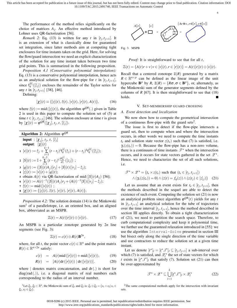
Proposition 4.2: The solution domain (14) is the Minkowskisum1 of a parallelotope, i.e. an oriented box, and an alignedbox, abbreviated as an MSPB.

Z(t) = A(t)[r](t)⊕ [v](t). (17)

An MSPB is a particular zonotope generated by 2n linesegments (see Fig. 3):

Z(t) = c(t)⊕R(t)B2n, (18)

where, for all t, the point vector c(t)∈Rn and the point matrixR(t) ∈ Rn×2n satisfy:

c(t) = A(t)mid([r](t))+mid([v](t)), (19)R(t) = [A(t)dr([r](t)) | dr([v](t))] . (20)

where | denotes matrix concatenation, and dr(.) is short fordiag(rad(.)), i.e. a diagonal matrix of real numbers eachcorresponding to the radius of an interval number.

1Let ξ1,ξ2⊂Rn, the Minkowski sum of ξ1 and ξ2 is: ξ1⊕ξ2 = {s1+s2|s1 ∈ξ1,s2 ∈ ξ2}.

Fig. 3. MSPB

Proof: It is straightforward to see that for all t,

Z(t) = {A(t)r+ v |v ∈ [v](t),r ∈ [r](t)}= A(t)[r](t)⊕ [v](t).

Recall that a centered zonotope Z(R) generated by a matrixR ∈ Rn×p can be defined as the linear image of the unithypercube Bp by R, Z(R) = {Rσ ,σ ∈ Bp}, or, alternately, asthe Minkowski sum of the generator segments defined by thecolumns of R [67]. It is then straightforward to see that (18)holds.

V. SET-MEMBERSHIP GUARD CROSSING

A. Event detection and localization

We now show how to compute the geometrical intersectionof a continuous flow-pipe with the guard sets2.

The issue is first to detect if the flow-pipe intersects aguard set, then to compute when and where the intersectionoccurs, in other words we need to compute the time instantste and solution state vector z(te) such that (7) is satisfied, i.e.γe(z(te)) = 0. Because the flow-pipe has a non-zero volume,there is a continuum of time instants T ? when the intersectionoccurs, and it occurs for state vectors gathered in the set Z ?.Hence, we need to characterize the set of all such solutions,i.e.

T ?×Z ? = {te× z(te) such that (te ∈ [t j, t j+1])

∧ (γe(z(te)) = 0)∧ (z(t) = fq(z))∧ (z(t j) ∈ [z] j)} (21)

Let us assume that an event exists for te ∈ [t j, t j+1], thenthe methods described in the sequel are able to detect theexistence of such event. Computing the solution set (21) is nowan analytical problem since algorithm ϕQR(t) yields for any tin [t j, t j+1] an analytical solution for the tube of trajectoriesover the time interval [t j, t j+1], hence the method described insection III applies directly. To obtain a tight characterizationof (21), we need to partition the search space. Therefore, tocurb computational complexity and keep it polynomial time,we further use the guaranteed relaxation introduced in [55]: weuse the algorithm Interval-Solve presented in section IIIbut bisect only along the single direction of the time variableand use contractors to reduce the solution set at a given timeinstant.

Let us denote [t?]l = [t?, t?]l ⊆ [t j, t j+1] a sub-interval overwhich (7) is satisfied, and Z ?

l the set of state vectors for whicht exists in [t?, t?]l that satisfy (7). Solution set (21) can thenbe over-approximated by

T ?×Z ? ⊆L⋃

l=1

[t?, t?]l×Z ?l (22)

2The same computational methods apply for the intersection with invariantsets.



7

Z

Z jCl

Z j+1

tt j t j+1

γe(.) = 0Z

Z jCl

Z j+1

tt j t? t j+1

γe(.) = 0

Fig. 4. Illustration of our intersection computation algorithm

where L is the number of solution sub-boxes. Finally, our ideais to contract the flow tube over tiny time slots to compute thesmallest solution boxes enclosing the intersection between thetube and the guard set, as depicted in Fig. 4.

Allowing some over-approximation when computing te,we say that an event occurs over the subinterval [t?, t?]l ifwid([t?, t?]l) is smaller than a given threshold εT , as suggestedin [46]. Now the question remains about how to compute atight over-approximation of Z ?

l . We solve this issue by solvinga constraint satisfaction problem as in [55]. This resolutionis repeated for l = 1, . . . ,L. Recall that the enclosure of thesolution of (5), which is an Initial Value Problem ODE, canbe computed for the small time interval [t?]l = [t?, t?]l in thecompound form (16), denoted [χ]l , using an inclusion functionfor algorithm ϕQR(t), which we obtain by using an interval [t]as input. We save the notation [χ?]l for the compound formcharacterizing the tight over-approximation of Z ?

l . We have

[χ]l = {[z]l , zl , [v]l , [r]l , A?l }. (23)

Let us assume that wid([t?, t?])≤ εT . Therefore

(∃z ∈ [z]l s.t. γe(z) = 0) ⇒(∃v× r ∈ [v]l× [r]l s.t. γe(v+A?r) = 0), (24)

hence, computing the intersection over the time interval [t?]boils down to solving the CSP

El := (Cl , [v]l× [r]l) . (25)where Cl := (γe

(v+A?

l r)= 0). (26)

Using a contractor, we can obtain a tight over-approximationof Z ? as a compound form [χ?], i.e.

[v?]l× [r?]l = Contractor(Cl , [v]l× [r]l). (27)

Here, we use the forward-backward contractor implemented inthe HC4_Revise method of the IBEX toolbox (www.ibex-lib.org) [65]. In fact, since the guard-set condition (7) isnaturally defined in the axis-aligned z−space and the trajectorytube is defined as an MSPB, we need to map the solutionof (7) naturally characterized in the z−space into the MSPBv× r−space; as implied in (24). Doing so, we inevitablyintroduce over-approximation. To curb the latter, the idea is tocombine the solutions of two contractors as now commonlydone when building solvers for CSPs (see [57], pp.90). There-fore, constraint (26) is rewritten using redundant constraints asfollows

C Rl := (γe

(v+A?

l r)= 0)∧ (γe

(z) = 0)∧ (z = v+A?

l r), (28)

whose solution is obtained via

[v?]l× [r?]l× [z?]l =Contractor(C Rl , [v]l× [r]l× [z]l). (29)

If the solution set for CSP (29) is not empty, we assume thatthe event e = q→ q′ occurs at te = t? and that [χ](t−e ) = [χ?]l ,as suggested in [46]. The discrete transition can then be com-puted from there, using the reset function ρe. The performanceof the set computation of the reset function is addressed in thenext subsection.

B. Set-membership reset mapping

Let us consider a sub-box Z ?l , l ∈ 1, ...,L, among those

defined in (22). After reset, the continuous transition resumesfrom the set Z ?′

l = ρe(Z ?l ). Since our continuous reachability

tool works with sets characterized as MSPBs, we need tocharacterize Z ?′

l as an MSPB. The image of a zonotope bya nonlinear mapping is not, in general, a zonotope. But usingmethods described in [68] and recalled in section III-D, wecan compute a tight bounding zonotope for Z ?′.

Our method for set-membership reset mapping uses theproperties of zonotopes given in section III-D as explainedbelow.

Theorem 3 (Nonlinear reset of an MSPB): Given a solutionbox in MSPB form Z ? = A[r]+ [v], the image Z ?′ = ρ(Z ?)is contained in an MSPB computed as follows

Z ?′ ⊆ A′[r]′+[v]′ (30)

where

A′ = J(:,1 : n) ∈ Rn×n, (31)[r]′ = Bn ⊆ Rn, (32)[v]′ = ρe(c)+�(J(:,n+1 : 3n)B2n)⊆ Rn, (33)

where �(.) denotes the convex hull of a set. Matrix J is definedby

J = sort(J), J = [mid([∇ρe]R) |G] ∈ Rn×3n, (34)

where sort(.) operator sorts the columns of a matrix accordingto their norm, vector c is defined in (19), matrix R ∈Rn×2n in(20), and matrix G ∈ Rn×n given by (12), with m = 2n. HereJ(:,1 : n) denotes the n first column vectors of matrix J, andJ(:,n+1 : 3n) the 2n last column vectors of matrix J.

Proof: From (18), we have Z ? = A[r]+ [v] = c⊕RB2n.By theorem 2, we have ρe(Z ?) = ρe(c)⊕♦([∇ρe(Z ?)R]B2n),then by theorem 1, ρe(Z ?) = ρe(c)⊕JB3n, where J is definedby (34). After sorting column vectors of J according to theirnorm, one obtains J. It is then straightforward to derive (30)-(34).

VI. ENCLOSING TIGHTLY A UNION OF TUBES

As stated in the previous section, the partition conductedwithin the event detection and localization phases yields manysolutions boxes which, after a set-membership reset mapping,are the initial state subsets for continuous transitions in thenew hybrid mode. Even if our algorithm performs a fast guardcrossing at low numerical cost, the computation of all thesetrajectory sub-tubes increases undesirably the computation



8

time. One solution consists in merging these sub-tubes intoa single tube enclosing their union. Since our method forcontinuous transitions, i.e. algorithm ϕQR(.) in algorithm 2uses MSPBs, a form consistent with the internal representationused by our continuous reachability algorithm, we obviouslyneed to compute the union of these sub-tubes in the form ofan MSPB.

The method we propose for merging the set of sub-tubesworks in three steps:• First, it computes the vertices of the convex domain

containing the union of the MSPBs describing the sub-tubes;

• Then, it computes a parametrized MSPB enclosing thesevertices;

• Finally, it tunes the MSPB parameters in order to optimizethe size of the resulting bounding MSPB.

These steps are described in the sequel.

A. Computing the sub-tubes vertices

Let us assume that the hybrid transition under study hasbeen completed and the initial domain for the continuoustransition in the new hybrid mode is characterized by thefollowing union of MSPB:

L⋃j=1

Z ?′l (35)

Each of the L MSPB solution domains, Z ?′l , l = 1 to L,

obtained via (30), is characterized as:

Z ?′l = {Alr+ v |v ∈ [v]l ,r ∈ [r]l}= Al [r]l +[v]l = cl⊕Z(Rl),

(36)where Z(Rl) is the centered zonotope generated by matrix Rl ∈Rn×2n, and where cl and Rl are defined from [v]l and [r]l asin (19)-(20).

Definition 1: Let R∈Rn×p be a matrix and let Z(R)=RBp⊂Rn be the centered zonotope generated by R. We denote byZ±(R), the set of point-vectors obtained as the linear imageby R of the 2p vertices of the unit hypercube Bp:

Z±(R) = {Rσ ,σ ∈ {−1,1}p}. (37)

Proposition 6.1 (Containment property): Let C (.) (resp.V (.)) denote the convex hull (resp. the vertices) of anypolytopic set. For all R ∈ Rn×p, we have:

V (Z(R))⊆ Z±(R), (38)C (Z±(R)) = Z(R), (39)p = 2n ⇒ ∃Rg ∈ Rn×p,

2card(V (Z(R)))≤ card(V (Z±(R)))≤ 2card(V (Z(Rg)))(40)

In words, Z±(R) contains all the vertices of Z(R), Z(R) is theconvex hull of Z±(R), and Z±(R) only contains twice morepoints than the true number of vertices of a MSPB (i.e. Z(Rg)with p = 2n) in the general case (i.e. non degenerate case)yielding equalities instead of inequalities in (40).

Proof: Properties (38)-(40) directly follow from defini-tion 1 and the convexity of zonotopic domains. (40) results

Fig. 5. Building the point-vectors cl +Z±(Rl)

from the maximum number of vertices of a p-zonotope in Rn,2∑

n−1i=0

(p−1

i

), which equals 2(2n−1) when applied to a MSPB

(p = 2n). By comparison, the number card(Z±(R)), (37), ofpotential vertices of a MSPB in Rn is 2p = 22n, so only twicemore than the true number of vertices of a generic MSPB, theratio being independent on n.

The next theorem formalizes the approach which supportsour method for enclosing a set of sub-tubes.

Theorem 4: Let M be a convex set (e.g. polytope, zonotope,MSPB, etc.). Consider the MSPB Z ?′

l in (36) and remind (19)-(20). Let P be a set of point-vectors obtained as follows:

P =L⋃

j=1

(cl +Z±(Rl)

), (41)

then, P ⊆M ⇒(⋃L

j=1 Z ?′l

)⊆M (42)

In words, any convex set M containing the point-vectors inP also contains the union of the MSPB domains Z ?′

l for l=1to L.

Proof: The proof of theorem 4 mainly relies on thepolytopic (thus convex) nature of the MSPB domains Z ?′

l =Al [rl ]+ [vl ] = cl ⊕Z(Rl) where cl ∈ Rn and Rl ∈ Rn×2n. (41)not only provides a constructive way to compute the m22n

point-vectors in P , but also ensures through (38) that Pcontains the set V of all the vertices of all the MSPB domainsZ ?′

l , l = 1, . . . ,L. In addition, (39) ensures that any convex setM satisfying P ⊆M also satisfies the containment propertyZ ?′

l ⊆M for each l=1 to L.Remark 3: Since Z±([R1,R2]) = Z±(R1)⊕ Z±(R2), the set

of point-vectors P defined in (41) can also be expressed asP =

⋃Ll=1(Al [r]±l ⊕ [v]±l

)where [r]±l and [v]±l refer to the set

of vertices of the n-dimensional axis-aligned boxes [r]l and[v]l , respectively. For a given value of l, figure 5 illustrates howthe set of points cl +Z±(Rl) can be built from Al [r]±l ⊕ [v]±l .

B. Enclosing a point-vector cloud by a zonotope

This subsection describes our generic algorithmcloud2zonotope (Algorithm 3) for computing thecenter c ∈ Rn and the shape matrix R ∈ Rn×p of a zonotopec⊕Z(R) enclosing a cloud X of N point-vectors defined in Rn.For better algorithm readability, vectors are explicitly denotedusing arrows ~u in the algorithms and in this subsection.

The algorithm cloud2zonotope (algorithm 3), also il-lustrated in Fig. 6, is mainly based on iterative compressions ofthe initial cloud X formed by N point-vectors and, jointly, theiterative building of the zonotope enclosure. After centeringthe cloud (step 5) in the middle of its interval hull (step 4),



9

each compression (step 9) is performed according to a vector~g∈Rn which further defines one of the generator segments ofthe resulting zonotope (step 10). At each iteration,~g is orientedalong the principal direction ~u of the current (i.e. partiallycompressed) cloud (step 7). Moreover, the magnitude of ~gis a fraction of (an approximation of) the largest projectionof the points in the (centered) cloud along ~u. The fractionused is defined by the scalar compression ratio, denoted ratio(ratio∈ [0,1]), and the approximation of the largest projectionrelies on a very fast computation based on the interval hullof the current cloud which corresponds to the scalar product~u · ~rad involving only two n-dimensional vectors at step 8.

Each iteration of the while loop in cloud2zonotopejointly performs a cloud compression, both in direction andmagnitude, as defined by generator ~g, and an expansion of thezonotope under construction, which relies on the Minkowskisum with the straight line segment [−1,+1]~g at step 10.Moreover, the function computing an updated cloud X =compress(X ,~g) from the compression of X in direction ~g,described in Algorithms 4, is designed so as to satisfy

X ⊂ (X⊕~g[−1,+1]), (43)

where matrices X and X are each identified to a set ofN point-vectors. Note that (43) is a key point to furtherensure that the initial cloud is enclosed within the zonotopeeventually returned by algorithm cloud2zonotope. Thejoint/iterative “cloud compression and zonotope expansion”process is repeated until one of the two stopping criteria s1 ors2 are satisfied (step 11): s1 is an integer defining the maximumnumber of allowed iterations, and s2 ∈ [0,1] is a positivereal number defining a stopping condition for the iterativecompressions in the form of a fraction of the initial cloudradius (~w assigned at step 6). After exiting from the while loop,the interval hull of the residual cloud is computed (step 13) andthe corresponding aligned box is summed (Minkowski sum)with the zonotope previously expanded from an initially emptyset during the while loop iterations. This results at step 14 intoa zonotope c⊕Z(R) which is guaranteed to contain all the Npoint-vectors defined by X when calling cloud2zonotope.

Fig. 6 illustrates the main steps of algorithm 3cloud2zonotope in the case of a 2-dimensional pointcloud and an MSPB output. Fig. 6.a shows that our algorithmfirst centers the point-vector cloud, then compresses the cloudalong the first principal direction ~u1. Here one can see point-vectors~z1 and~z2 projected onto axis ~u1 while considering thebound defined by ratio. Thus, compressing the cloud boilsdown to keeping only the difference~zδ

i =~zi−~zgi . Fig. 6.b shows

the point-vector cloud after the first compression along direc-tion ~u1. Our algorithm finds the next compression direction ~u2as the first principal direction of the remaining cloud. In orderto obtain an MSPB as output set, the number of compressioniterations is taken as n = 2 ; Fig. 6.c shows that after n = 2compression iterations, the residual point-vectors are enclosedwithin an axis-aligned box. Fig. 6.d shows the zonotope, herean MSPB obtained as the Minkowski sum of the axis-alignedbox and the parallelotope as defined by the generator segments~g1 = ‖~g1‖~u1 and ~g2 = ‖~g2‖~u2.

−4 −2 0 2 4

−3

−2

−1

0

1

2

3

x

y

2.ratio

~g~z1

C

~u1

~z⊥1

~zg2

~zg1

~z⊥2

~z2

(a) Cloud centering and compression along first principal direction

−4 −2 0 2 4

−3

−2

−1

0

1

2

3

x

y

~u2 ~u1

(b) Finding the second compression direction as the first principaldirection of the remaining cloud.

−5 0 5

−3

−2

−1

0

1

2

3

x

y

(c) Enclosing the residual pointcloud in an axis-aligned box.

−5 0 5

−3

−2

−1

0

1

2

3

x

y

(d) Computing the MSPB enclosingthe point cloud.

Fig. 6. Main steps for build the enclosing zonotope as performed byAlgorithm 3 cloud2zonotope in the case of a 2D point cloud and anMSPB output.

C. Building the MSPB from the zonotope enclosure

Using algorithm cloud2zonotope, one can tune param-eters ratio and si, i = 1,2 introduced in the latter section, inorder to obtain a particular zonotope with center cM and shapematrix RM ∈Rn×2n representing the tightest MSPB enclosingthe point cloud P defined in (41). Choosing s1=n and s2=0,algorithm cloud2zonotope yields an MSPB since thereare exactly n compression iterations, hence exactly n generatorvectors. Moreover, the remaining cloud is eventually gathered



10

in an axis-aligned box. The size of the MSPB solely dependson parameter ratio that can be tuned to optimize any size-based criterion. The latter tuning acts as a trade-off betweenthe relative weight of the parallelotope and the axis-alignedbox in (17). The optimal choice for the parameter ratio isthen formally given as

ratio?ratio∈[0,1]

= argmin µ(Z(R)) (44)

where µ(.) is the size of the zonotope. The optimal choicecan be obtained in three ways : volume minimization, segmentminimization, or P-radius minimization.

1) Volume minimization: The volume of a zonotope [69]Z(R)⊂Rn, where R = [r1, . . . ,rp]∈Rn×p, with p≥ n, is givenby:

Vol(Z(R)) = 2n( ∑1≤i1≤i2≤...in≤p

|det([ri1 , . . . ,rin ])|) (45)

The integers i1, . . . , in correspond to different ways of choosingn elements amongst p. The sum (45) is thus composed of(

pn

)elements.

2) Segment length minimization: The segment’s length ofa zonotope Z= c⊕RBp ∈ Rn is given by the sum of squaresof the generators of the zonotope Z. Computing the sum ofsquares of the generators of the zonotope Z boils down tocomputing the Frobenius norm of R.

Sm(Z(R)) =n

∑i=1

p

∑i=1

R2i j = ‖R‖2

F = Tr(R>R) (46)

where Tr denotes the trace of a square matrix.3) P-radius minimization: The P-radius [11] of a zonotope

Z= c⊕RBp ∈ Rn is defined as

Prad(Z(R)) = maxx∈Z‖x− c‖2

P = maxx∈Z

(x− c)>P(x− c) (47)

where P = P> ≥ 0 is a symmetric and positive definite matrix.To obtain the solution ratio? one can use an iterative algo-

rithm, possibly using derivatives obtained via finite difference.Here, we merely evaluate the size of the MSPB for ten valuesof ratio taken over a grid of values between 0 and 1, and thenmerely pick up the value which minimises (44).

Summarizing, the union of L MSPB solution domains asdefined by (35) is tightly enclosed into a single MSPB of op-timized size, and obtained with algorithm cloud2zonotopetuned with ratio=ratio?, s1=n and s2=0.

VII. PROPERTIES AND COMPLEXITY ANALYSIS

Our hybrid reachability method alternates an interval Taylorintegration method implementing Lohner’s QR-factorisationfor the continuous expansion of the hybrid system and anoriginal method for guard crossing materialized by transitions.

Proposition 7.1 (Conservative hybrid reachability): Thehybrid reachability algorithm provides guaranteed outputs, i.e.the flow-pipe generated by alternating continuous reachability(Algorithm 2: ϕQR), flow guard intersection (Algorithm 6:hybrid-transition) and trajectory fusion (Algorithm 5:MSPB) is guaranteed in the sense that it encloses all thetrajectories of the hybrid system HA (1) consistent with the

Algorithm 3: Algorithm cloud2zonotope

Input : X := {~xi, i = 1 . . .N}, ratio ∈ [0,1], s1, s2Output: ~c ∈ Rn, R ∈ Rn×p

1 Initialization: ~c = 0, R = /0, iter = 0, ~w = 0;2 while (iter < s1)∨ (∃i ~radi > s2~wi) do3 update iteration counter. iter := iter+1 ;4 compute cloud center and radius.

{ ~mid, ~rad} := minbox(X) ;5 center point-cloud around mid. X := X− ~mid ;6 store initial radius. if iter = 1 then ~w := ~rad;7 find first principal direction (unit vector ~u).

(U,S) := svd(X), ~u :=U(:,1) ;8 choose generator segment. ~g := ratio|~u · ~rad| ·~u ;9 compress cloud along ~g using ratio.

X := compress(X ,~g) ;10 update zonotope generators. ~c :=~c+ ~mid, R := [R, ~g]11 end while12 enclose remaining cloud in a box.{~mid,~rad} := minbox(X) ;

13 update zonotope. ~c :=~c+ ~mid, R := [R, diag( ~rad)] ;

Algorithm 4: Algorithm compress

1 Function X=compress(X, ~g)2 compute compression direction. ~u =~g/‖~g‖;3 for each point-vector ~xi in X do4 compute coordinates along ~u. d :=~xi ·~u ;5 compression along ~u.

d := min(‖~g‖,max(−‖~g‖,d));6 update coordinates. ~xi =~xi−d~u ;7 end for8 return

Algorithm 5: Algorithm MSPB

Input : LOutput: Linitialization: P = /0 i.e. empty set of points ;for j← 1 to Length(L ) do

pick up Z ?′l from L (i.e. q, Al , [r]l , [v]l);

P := P ∪(Al [r]±l ⊕ [v]±l

)end forXP := matrix representation (n col.) of P ⊂ Rn ;for ratio =: 0,0.1, . . . ,0.9,1 do{cM ,RM } := cloud2zonotope(XP ,ratio,n,0) ;compute the size of zonotope µ(Z(RM )) as in (45);

end forr∗ := argmin µ(Z(RM )) ;extract MSPB attributes of M ∗ := cM ∗ ⊕Z(RM ∗)obtained with r∗:A := RM ∗(:,1 : n) ;[r] := [−1,+1]n ;[v] := cM ∗ +diag(RM ∗(:,(n+1) : (2n)))[−1,+1]n ;store MSPB: L := (q,A, [r], [v]) in list L ;



11

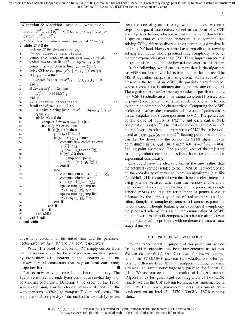
Algorithm 6: Algorithm Hybrid-Transition

input : L Fj , t j+1,{ϕQR

q (), ϕq()}q∈Q , {γe(),ρe()}e∈E , εT

output: L Fj+1, L

Rj+1

1 Initialization : initialize running frontier list L := L Fj ;

33 while L 6= /0 do4 pick up L list element (q, t0, [χ0]);5 /* Continuous transition */6 compute continuous expansion over [t0, t j+1]→ [z] j;7 update reached set list L R

j+1← (q, t0, t j+1, [z j]);8 compute new solution at time t j+1→ [χ j+1];9 solve CSP to compute [χ ′j+1] := [χ j+1]∩ inv(q);

10 if [χ j+1]′ 6= /0 then

11 update frontier list L Fj+1← (q, t j+1, [χ j+1]

′);12 end if13 if Length(L F

j+1 > 2) then14 L F

j+1 := MSPB(L Fj+1)

15 end if16 /* Discrete transition */17 forall the elements e← E do18 initialize running jump list Le := {(q, t0, [χ0], t j+1)};

t1 := t j+1;2020 while Le 6= /0 do21 compute flow over [t0, t1]→ [z];22 if e = (q,q′) exists then23 if (γe([z]) 3 0) then24 t? := t0 ; t? := t1;25 if ((t?− t?)≤ εT ) then26 compute flow enclosure over

[t?, t?]→ [χ];27 [χ]? := HC4 Revise([χ]);28 if [χ]? 6= /0 then29 jump and update

L ← (q′, t?,ρe([χ]?));

30 end if31 else32 compute solution set at t?→ [χ]1;33 compute solution set at

t1 := (t?+ t?)/2→ [χ]2;34 update running jump list

Le← (q, t?, [χ]1, t1);35 update running jump list

Le← (q, t1, [χ]2, t?);

36 end if37 end if38 end if39 end while40 end forall41 end while

uncertainty domains of the initial state and the parametervector given by X0 ⊆ Rn and P⊆ Rnp , respectively.

Proof: The proof of proposition 7.1 simply derives fromthe conservatism of the three algorithms involved provedby Proposition 4.1, Theorem 3, and Theorem 4, and theconservatism of contractors that rely on local consistencyproperties [65].

Let us now provide some hints about complexity. TheTaylor series method underlying continuous reachability is ofpolynomial complexity. Denoting k the order of the Taylorseries expansion, usually chosen between 10 and 20, thework per step is O(k2) to compute Taylor coefficients. Thecomputational complexity of the method hence mainly derives

from the one of guard crossing, which includes two mainsteps: flow guard intersection, solved in the form of a CSP,and trajectory fusion, which is solved by the algorithm MSPB,a specific kind of zonotope enclosure. It is admitted thatsolving CSPs, either on discrete or on continuous domains, isin theory NP-hard. However, there have been efforts to developsolving techniques whose practical time complexity is betterthan the exponential worst case [70]. These improvements relyon technical features that are beyond the scope of this paper.

In the following, we discuss in more details the algorithmfor MSPB enclosure, which has been tailored for our use. TheMSPB algorithm merges in a single reachability set M , ex-pressed in the form of an MSPB, the possibly many flowpipeswhose computation is initiated during the crossing of a guard.The algorithm cloud2zonotope makes it possible to buildthis MSPB (actually an n-dimensional zonotope) from a cloudof points (here, potential vertices) which are known to belongto the union domain to be characterized. Computing the MSPBenclosure involves the generation of a cloud of points and npartial singular value decompositions (SVD). The generationof the cloud of points is O(22n), and each partial SVDcomputation is O(Nn2). The cost of enumerating the N =m22n

potential vertices related to a number m of MSPBs can be eval-uated as f lPV−Enum(n,m)≈mn22n floating-point operations. Itcan then be shown that the cost of the MSPB algorithm canbe evaluated as f lMSPB(n,m)≈ m22n(40n3 +40n2 +n)+80n4

floating-point operations. The practical cost of the trajectoryfusion algorithm therefore comes from the vertex enumerationexponential complexity.

One could have the idea to consider the true (rather thanthe potential) vertices related to the m MSPBs. However, basedon the complexity of vertex enumeration algorithms (e.g. likeQuickHull [71]), it can be shown that there is a clear interest inusing potential vertices rather than true vertices enumeration:the former method only induces twice more points for a singlegeneric MSPB and this greater number of points is easilybalanced by the simplicity of the related enumeration algo-rithm, though the complexity remains of course exponentialin both cases. Though featuring an exponential complexity,the proposed scheme relying on the enumeration of MSPBpotential vertices can still compete with other algorithms (evenpolynomial ones) for problems with moderate continuous statespace dimension.

VIII. NUMERICAL EVALUATION

For the experimentation purpose of this paper, our methodfor hybrid reachability has been implemented as follows.We use the Profil/Bias C++ class for interval compu-tation, the FABDAB++ package (www.fadbad.com) for au-tomatic differentiation, AML++ (amlpp.sourceforge.net) andArmadillo (arma.sourceforge.net) package for Linear al-gebra. We use our own implementation of Lohner’s method(Algorithm 2) for guaranteed set integration of IVP ODE.Finally, we use the CSP solving techniques as implemented inthe IBEX C++ library (www.ibex-lib.org). Experiments wereconducted on an intel i5− 3470− 3.6GHz−16GB runningLinux.



12

TABLE I(P-radius,Sm , VOLUME) VS ratio FOR THE MASS-SPRING, FIRST SWITCH

ratio 0 0.1 0.2 0.3 0.4 0.5 0.6 0.7 0.8 0.9 1P-radius 1.910 1.910 1.910 1.910 1.915 1.929 1.926 1.929 1.936 1.946 1.962

Sm× (10−3) 4.646 3.174 2.002 1.823 1.792 2.179 2.329 2.729 3.331 4.149 5.115Volume ×(10−3) 8.574 3.417 1.104 1.961 3.122 4.974 5.511 2.445 3.239 4.745 6.577

TABLE II(P-radius,Sm , VOLUME) VS ratio FOR THE MASS-SPRING, SECOND SWITCH

ratio 0 0.1 0.2 0.3 0.4 0.5 0.6 0.7 0.8 0.9 1P-radius 0.710 0.710 0.710 0.710 0.710 0.710 0.710 0.710 0.713 0.725 0.737

Sm× (10−3) 8.641 6.116 4.094 3.781 3.950 3.653 4.048 4.769 5.899 7.403 9.122Volume ×(10−3) 16.186 7.444 1.295 3.290 6.273 8.838 9.979 5.088 6.383 9.413 13.053

A. Case study 1 : Switched mass-spring system

Consider the switched dynamical system with two modesq = 1, 2 and one jump transition e = 1 → 2 obtained byintroducing an artificial switching in a mass-spring system.The switching is artificial because continuous dynamics arethe same in the two modes. The main idea is to investigate theimpact of our guard crossing and trajectory merge algorithmsby comparing the results with the original continuous system,i.e. without switching.

The switched system is given by

flow(1) : f1(x1, x2) =(x2,

−km x1− c

m x2)

inv(1) : ν1(x1,x2) = x1− x2 < 0flow(2) : f2(x1, x2) = f1(x1, x2)inv(2) : ν2(x1,x2) =−ν2(x1,x2)< 0guard(1) : γ1(x1,x2) = x2− x1 = 0reset(1) : ρ1(x1,x2) = (α1x1,α2x2)

(48)

where α1 = α2 = 1, k = 4, m = 2, c = 1.25. The continuousstates are described by two variables (x1,x2), where x1, x2 re-spectively represent the position and the velocity of the mass-spring. The initial conditions are given by x1 ∈ [1,1.1], x2 ∈[−0.63,−0.61]. Algorithms Hybrid-Transition (Algo-rithm 6) and ϕQR (Algorithm 2 ) were tuned as follows : Thetime step is chosen constant h = 0.1; and the time interval isbisected until a threshold εT = 0.005.

Fig. 7 gathers the reachable sets as obtained for the timehorizon [0, 5]. First the reachable set for the original contin-uous system is shown, then the one for the switched versionwithout trajectory merge. Then the reachable set as obtainedwith our trajectory merge algorithm using one of the severalcriteria proposed in section VI-C: P-radius, with P takenas identity matrix, volume and segments length. Tables I-IIshows the criteria obtained for the first and second switchesrespectively. The optimal tuning parameter clearly depends onthe criterion, though it does not seem to change significantlywith the switching. The bottom right graph in Fig. 7 clearlyshows that the P-radius criterion yields the tightest MSPB,but still with significant over-approximation compared to theenclosure computed for the continuous system (i.e. withoutswitching). Nevertheless, the MSPB obtained with our mergealgorithm are always significantly tighter than the enclosureobtained using naive convex interval hull of trajectory tubes.

-2

-1.5

-1

-0.5

0

0.5

1

-0.5 0 0.5 1

X2

X1-2

-1.5

-1

-0.5

0

0.5

1

-0.5 0 0.5 1

X2

X1-2

-1.5

-1

-0.5

0

0.5

1

-0.5 0 0.5 1

X2

X1

-2

-1.5

-1

-0.5

0

0.5

1

-0.5 0 0.5 1

X2

X1-2

-1.5

-1

-0.5

0

0.5

1

-0.5 0 0.5 1

X2

X1-2

-1.5

-1

-0.5

0

0.5

1

-0.5 0 0.5 1

X2

X1

-2

-1.5

-1

-0.5

0

0.5

1

-0.5 0 0.5 1X2

X1

0

0.1

0.2

0.3

0.4

0.5

0.6

0.7

0.8

-0.1 0 0.1 0.2 0.3 0.4 0.5 0.6

X2

X1

VolumeP-radius

Segment-MinRadius=0

ContinuousConvex Hull

Fig. 7. The frontier, i.e. the solution sets at time-grid points for the Mass-Spring. From left to right, and top to bottom, the continuous version (CPU0.007s), the switched version without trajectory merging (CPU 0.88s), theswitched version with trajectory merging using P-radius criterion (CPU0.125s), using segment length criterion (CPU 0.129s), using volume criterion(CPU 0.163s), when merging with ratio=0 (CPU 0.202s), and using naiveconvex hull (CPU 0.133s). The final graph compares the MSPB solutionenclosure obtained at final time for the different experiments.

B. Case study 2 : A ball bouncing on a sinusoidal surface

We consider the uncertain model of a ball that bounces ona sinusoidal surface (modified from [54]). It is described byfour variables (px, py,vx,vy), where (px, py) is ball positionin 2D and (vx,vy) ball velocity. Figure VIII-B provides thehybrid automaton of the system. Model parameters are set tog ∈ [9.8,9.85], e = 3.5 and k ∈ [0.3,0.4] (all units are S.I).We took a constant integration time step h = 0.1 for ϕQR



13

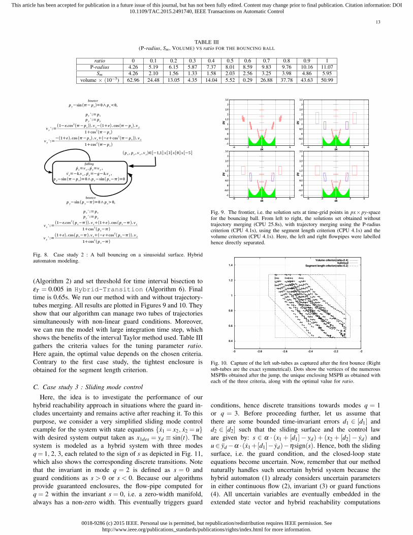
TABLE III(P-radius, Sm , VOLUME) VS ratio FOR THE BOUNCING BALL

ratio 0 0.1 0.2 0.3 0.4 0.5 0.6 0.7 0.8 0.9 1P-radius 4.26 5.19 6.15 5.87 7.37 8.01 8.59 9.83 9.76 10.16 11.07

Sm 4.26 2.10 1.56 1.33 1.58 2.03 2.56 3.25 3.98 4.86 5.95volume × (10−3) 62.96 24.48 13.05 4.35 14.04 5.52 0.29 26.88 37.78 43.63 50.99

3

Fig. 8. Case study 2 : A ball bouncing on a sinusoidal surface. Hybridautomaton modeling.

(Algorithm 2) and set threshold for time interval bisection toεT = 0.005 in Hybrid-Transition (Algorithm 6). Finaltime is 0.65s. We run our method with and without trajectory-tubes merging. All results are plotted in Figures 9 and 10. Theyshow that our algorithm can manage two tubes of trajectoriessimultaneously with non-linear guard conditions. Moreover,we can run the model with large integration time step, whichshows the benefits of the interval Taylor method used. Table IIIgathers the criteria values for the tuning parameter ratio.Here again, the optimal value depends on the chosen criteria.Contrary to the first case study, the tightest enclosure isobtained for the segment length criterion.

C. Case study 3 : Sliding mode control

Here, the idea is to investigate the performance of ourhybrid reachability approach in situations where the guard in-cludes uncertainty and remains active after reaching it. To thispurpose, we consider a very simplified sliding mode controlexample for the system with state equations {x1 = x2, x2 = u}with desired system output taken as x1des = yd ≡ sin(t). Thesystem is modeled as a hybrid system with three modesq = 1, 2, 3, each related to the sign of s as depicted in Fig. 11,which also shows the corresponding discrete transitions. Notethat the invariant in mode q = 2 is defined as s = 0 andguard conditions as s > 0 or s < 0. Because our algorithmsprovide guaranteed enclosures, the flow-pipe computed forq = 2 within the invariant s = 0, i.e. a zero-width manifold,always has a non-zero width. This eventually triggers guard

-1

-0.5

0

0.5

1

1.5

2

2.5

3

3.5

-6 -3 0 3 6

py

px

-1

-0.5

0

0.5

1

1.5

2

2.5

3

3.5

-6 -3 0 3 6

py

px

-1

-0.5

0

0.5

1

1.5

2

2.5

3

3.5

-6 -3 0 3 6

py

px

-1

-0.5

0

0.5

1

1.5

2

2.5

3

3.5

-6 -3 0 3 6

py

px

Fig. 9. The frontier, i.e. the solution sets at time-grid points in px× py-spacefor the bouncing ball. From left to right, the solutions set obtained withouttrajectory merging (CPU 25.8s), with trajectory merging using the P-radiuscriterion (CPU 4.1s), using the segment length criterion (CPU 4.1s) and thevolume criterion (CPU 4.1s). Here, the left and right flowpipes were labelledhence directly separated.

0.4

0.6

0.8

1

1.2

1.4

-3 -2.8 -2.6 -2.4 -2.2 -2

Volume criterion(ratio=0.4)hullcloud

Segment length criterion(ratio=0.2)

Fig. 10. Capture of the left sub-tubes as captured after the first bounce (Rightsub-tubes are the exact symmetrical). Dots show the vertices of the numerousMSPBs obtained after the jump, the unique enclosing MSPB as obtained witheach of the three criteria, along with the optimal value for ratio.

conditions, hence discrete transitions towards modes q = 1or q = 3. Before proceeding further, let us assume thatthere are some bounded time-invariant errors d1 ∈ [d1] andd2 ∈ [d2] such that the sliding surface and the control laware given by: s ∈ α · (x1 + [d1]− yd) + (x2 + [d2]− yd) andu∈ yd−α ·(x1+[d1]− yd)−ηsign(s). Hence, both the slidingsurface, i.e. the guard condition, and the closed-loop stateequations become uncertain. Now, remember that our methodnaturally handles such uncertain hybrid system because thehybrid automaton (1) already considers uncertain parametersin either continuous flow (2), invariant (3) or guard functions(4). All uncertain variables are eventually embedded in theextended state vector and hybrid reachability computations



14

q = 1s < 0

q = 2s = 0

q = 3s > 0

s = 0

s < 0

s > 0

s = 0

Fig. 11. The hybrid automaton for the sliding mode control under study

Fig. 12. The reachable set for the sliding mode control trajectory tracking.On the same graph, time-history of x1-variable (starts at 1), x2-variable (startsat 0) and s (reaches 0 and stays there). Left: with no uncertainty (34s CPU).Right: with uncertainty (97s CPU).

use equations (5-7). Here, we took a constant integrationtime step h = 0.005s for ϕQR (Algorithm 2) and used notime interval bisection in Hybrid-Transition (Algorithm6). α = 0.01 and η = 0.5. Final time is 20s. We run ouralgorithm with trajectory-tube fusion using the segment-lengthcriterion, and obtained the reachable set plotted in Fig. 12.Notice system trajectories obtained without uncertainty, i.e.[d1] = [d2] = {0}, and the ones with uncertainty taken as[d1] = [d2] = [−0.02,0.02]. Starting with (1,0) as initial condi-tions, the system reaches the uncertain sliding surface at timet = 2s and remains there until simulation ends. It is clear thatour algorithm can manage situations where the guard remainsactive after reaching it, and that it also characterizes efficientlythe impact of any uncertainty acting either on the flow or onthe guard condition. The thickness that appears in system statetrajectories when they reach the sliding surface is induced bythe bounded uncertainties [d1] and [d2] influencing the slidingsurface.

D. Case study 4 : Nonlinear hybrid system of high dimension

The purpose is to investigate the scalability of our trajectorymerge approach within our hybrid reachability method. Weconsider the switched dynamical system with two modes q =1, 2 and one jump transition e= 1→ 2 obtained by introducingan artificial switching in the dynamical model of an oscillatorynetwork of transcriptional regulators with N genes [72]. Letus denote ~x = (m1, p1, . . . , mi, pi, . . . , mN , pN) the continuousstate vector. The guard condition is given by the nonlinearcondition γ1(~x) = 0, with

γ1(~x) =i=2N

∑i=1

(xi−5)2− r2

and r = 75, and the continuous dynamics are described by theODE ~x = f (~x) in the form

i = 1, . . . ,N

{mi = −mi +bpi +

α(t)1+pn

i−1+α0

i (t)

pi = κ(t)mi−µ(t)pi(49)

TABLE IVSCALABILITY OF THE HYBRID REACHABILITY METHOD. COMPUTATION

TIMES IN SECONDS (AVERAGE OF 10 RUNS - CASE STUDY 4).

Without Hybrid Hybrid2N artificial switching without fusion with fusion2 0.42 98.4 3.944 0.935 337 22.36 1.44 740 64.4

10 2.87 796 10512 3.77 1197 13014 4.78 1814 34716 5.91 2076 NA18 7.16 3460 NA24 11.75 5113 NA

Fig. 13. The reachable set for system (49) with 2N=12. Left, time-history ofm1-variable, Right, time-history of p1-variable.

with b =−0.5, n = 2 and p0 = pN . We assume that the func-tions α(t), κ(t), µ(t), and α0

i (t), are unknown but bounded,and the bounds are as follows: for all t, α(t) ∈ [0.5, 1.5],κ(t)∈ [1.9, 2.1], µ(t)∈ [1.9, 2.1] and for all i α0

i (t)∈ [25, 26].Initial conditions are taken as: m3k+1(t0)∈ [35,40], p3k+1(t0)∈[27,32], m3k+2(t0) ∈ [30,35], p3k+2(t0) ∈ [25,30], m3k+3(t0) ∈[40,45], p3k+3(t0) ∈ [32,37], for k=0 to 7. Algorithm ϕQR

(Algorithm 2) was run with a constant integration time steph = 0.01min and algorithm Hybrid-Transition (Algo-rithm 6) was run with no time interval bisection. Final timeis 10min. The trajectory merge is done with the segmentlength criterion. Fig. 13 depicts the reachable sets as obtainedwith 2N = 12. Table IV gathers the computation times forsettings with 2N ranging from 2 to 24. Computations withour fusion algorithm were successful for values of 2N upto 14. For larger values of N, the memory size required bythe enumeration of potential vertices exceeds the availableone. Nevertheless, comparing the simulation runs with andwithout merging clearly demonstrates the usefulness of ourapproach since computation times in these settings have beenreduced by factor 5 for systems with continuous dimensionas large as 14. Comparing the continuous simulation and thehybrid with trajectory merge gives an insight about the overallcost of our method for crossing nonlinear guards. For higherdimensions, further investigations are needed to counteract theimpact of the exponential complexity of vertices enumerationin the fusion algorithm.

IX. CONCLUSION AND FUTURE WORKS

We have addressed hybrid reachability analysis of uncertainnonlinear hybrid systems using interval analysis, guaranteedset integration, interval constraint propagation and geometricaltools based on zonotopes. Continuous transitions are addressed



15

using state-of-the-art methods for guaranteed and validatedset integration. Discrete transitions use first a method forreliable event detection and localization that is based on aone-dimensional bisection strategy allied with zonotope-basedgeometrical tools for domain computation. It then relies onzonotope/MSPB bounding to enclose the flow-pipes obtainedafter a jump, in a form consistent with our continuousreachability approach. The bounding approach relies on aparameter that is tuned on-the-fly. The method, evaluated onnonlinear hybrid systems, has shown promising performanceand reasonable computation times, even under continuous statedimensions greater than ten. Further work will focus on waysto improve the approach’s scalability, and detect and mergenon-connected clouds of flow-pipes, and also on the possibilityto use a paving using MSPB to cover large solution sets.

REFERENCES

[1] R. Gonzalez, M. Fiacchini, T. Alamo, J. Guzman, and F. Rodriguez,“Online robust tube-based MPC for time-varying systems: a practicalapproach,” International Journal of Control, vol. 84, no. 6, pp. 1157–1170, 2011.

[2] S. Rakovic, B. Kouvaritakis, M. Cannon, C. Panos, and R. Findeisen,“Parameterized tube model predictive control,” Automatic Control, IEEETransactions on, vol. 57, no. 11, pp. 2746–2761, 2012.

[3] J. K. Scott and P. I. Barton, “Bounds on the reachable sets of nonlinearcontrol systems,” Automatica, vol. 49, no. 1, pp. 93 – 100, 2013.

[4] J. Lygeros, “On reachability and minimum cost optimal control,” Auto-matica, vol. 40, no. 6, pp. 917–927, 2004.

[5] J. Lygeros, D. N. Godbole, and S. Sastry, “Verified Hybrid Controllersfor Automated Vehicles,” IEEE Transactions on Automatic Control,vol. 43, no. 4, pp. 522–539, 1998.

[6] C. J. Tomlin, J. Lygeros, and S. Sastry, “A Game Theoretic Approach toController Design for Hybrid Systems,” Proceedings of IEEE, vol. 88,pp. 949–969, Jul. 2000.

[7] L. de Alfaro, T. A. Henzinger, and O. Kupferman, “Concurrent reach-ability games,” Theor. Comput. Sci., vol. 386, no. 3, pp. 188–217, Oct.2007.

[8] Y. Gao, J. Lygeros, and M. Quincampoix, “The reachability problemfor uncertain hybrid systems revisited: A viability theory perspective,”in HSCC, 2006, pp. 242–256.

[9] N. Meslem, N. Ramdani, and Y. Candau, “Using hybrid automata forset-membership state estimation with uncertain nonlinear continuous-time systems,” Journal of Process Control, vol. 20, no. 4, pp. 481 –489, 2010.

[10] E. Benazera and L. Trave-Massuyes, “Set-theoretic estimation of hy-brid system configurations,” IEEE Transactions on Systems, Man, andCybernetics, Part B, vol. 39, no. 5, pp. 1277–1291, 2009.

[11] V. T. H. Le, C. Stoica, T. Alamo, E. F. Camacho, and D. Dumur, “Zono-topic guaranteed state estimation for uncertain systems,” Automatica,vol. 49, no. 11, pp. 3418 – 3424, 2013.

[12] F. Chernousko, “Ellipsoidal state estimation for dynamical systems,”Nonlinear Analysis: Theory, Methods Applications, vol. 63, no. 57, pp.872 – 879, 2005.

[13] H. Gueguen, M.-A. Lefebvre, J. Zaytoon, and O.Nasri, “Safety verifi-cation and reachability analysis for hybrid systems,” Annual Reviews inControl, vol. 33, no. 1, pp. 25 – 36, 2009.

[14] E. M. Clarke, A. Fehnker, Z. Han, B. H. Krogh, O. Stursberg, andM. Theobald, “Verification of hybrid systems based on counterexample-guided abstraction refinement,” in TACAS, 2003, pp. 192–207.

[15] C. J. Tomlin, I. M. Mitchell, A. M. Bayen, and M. Oishi, “Computationaltechniques for the verification of hybrid systems,” Proceedings of theIEEE, vol. 91, no. 7, pp. 986–1001, 2003.

[16] A. Aswani, J. Ding, H. Huang, M. Vitus, J. Gillula, P. Bouffard, andC. Tomlin, “Verification and control of hybrid systems using reachabilityanalysis with machine learning,” in HSCC ’12, 2012, pp. 1–2.

[17] A. Donze, B. Krogh, and A. Rajhans, “Parameter synthesis for hybridsystems with an application to simulink models,” in HSCC, ser. LNCS,2009, pp. 165–179.

[18] J. Lygeros, C. Tomlin, and S. Sastry, “On controller synthesis fornonlinear hybrid systems,” in IEEE CDC, vol. 2, 1998, pp. 2101–2106.

[19] R. Alur, T. Dang, J. Esposito, Y. Hur, F. Ivancic, V. Kumar, P. Mishra,G. Pappas, and O. Sokolsky, “Hierarchical modeling and analysis ofembedded systems,” Proceedings of the IEEE, vol. 91, no. 1, pp. 11–28, 2003.

[20] R. Alur, C. Courcoubetis, N. Halbwachs, T. A. Henzinger, P.-H. Ho,X. Nicollin, A. Olivero, J. Sifakis, and S. Yovine, “The algorithmicanalysis of hybrid systems,” Theoretical Computer Science, vol. 138,pp. 3–34, 1995.

[21] E. Asarin, O. Maler, and A. Pnueli, “Reachability analysis of dynamicalsystems having piecewise-constant derivatives,” Theoretical ComputerScience, vol. 138, pp. 35–66, 1995.

[22] A. Chutinan and B. Krogh, “Computational techniques for hybrid systemverification,” Automatic Control, IEEE Transactions on, vol. 48, no. 1,pp. 64–75, 2003.

[23] A. Girard, “Reachability of uncertain linear systems using zonotopes,”in HSCC, vol 3414 in LNCS, 2005, pp. 291–305.

[24] A. Girard and C. L. Guernic, “Zonotope/hyperplane intersection forhybrid systems reachability analysis,” in HSCC, 2008, pp. 215–228.

[25] M. Althoff and B. H. Krogh, “Avoiding geometric intersection operationsin reachability analysis of hybrid systems,” in HSCC, 2012, pp. 45–54.

[26] A. Kurzhanskiy and P. Varaiya, “Ellipsoidal techniques for reachabilityanalysis of discrete-time linear systems,” Automatic Control, IEEETransactions on, vol. 52, no. 1, pp. 26–38, 2007.

[27] L. Doyen, T. Henzinger, and J. Raskin, “Automatic rectangular refine-ment of affine hybrid systems,” in FORMATS’05, vol. 3829 in LNCS,2005, pp. 144–161.

[28] M.-A. Lefebvre and H. Guguen, “Hybrid abstractions of affine systems,”Nonlinear Analysis: Theory, Methods Applications, vol. 65, no. 6, pp.1150 – 1167, 2006.

[29] M. Kloetzer and C. Belta, “Reachability analysis of multi-affine sys-tems,” in HSCC, vol. 3927 in LNCS, 2006, pp. 348–362.

[30] R. Alur, T. Dang, and F. Ivancic, “Predicate abstraction for reachabilityanalysis of hybrid systems,” ACM Trans. Embed. Comput. Syst., vol. 5,no. 1, pp. 152–199, Feb. 2006.

[31] I. M. Mitchell, A. M. Bayen, and C. J. Tomlin, “A time-dependantHamilton-Jacobi formulation of reachable sets for continuous dynamicsgames,” IEEE Trans. Automatic Control, vol. 50, no. 7, pp. 947–957,2005.

[32] V. Shia, R. Vasudevan, R. Bajcsy, and R. Tedrake, “Convex computationof the reachable set for controlled polynomial hybrid systems,” in 53rdIEEE Conference on Decision and Control, 2014, pp. 1499–1506.

[33] M. Althoff, O. Stursberg, and M. Buss, “Reachability analysis of nonlin-ear systems with uncertain parameters using conservative linearization,”in CDC, 2008, pp. 4042–4048.

[34] G. Batt, C. Belta, and R. Weiss, “Model checking genetic regulatorynetworks with parameter uncertainty,” in HSCC, vol. 4416 in LNCS.Springer-Verlag, 2007, pp. 61–75.

[35] E. Asarin, T. Dang, and A. Girard, “Hybridization methods for theanalysis of non-linear systems,” Acta Informatica, vol. 43, pp. 451–476,2007.

[36] S. Burden, H. Gonzalez, R. Vasudevan, R. Bajcsy, and S. Sastry, “Nu-merical integration of hybrid dynamical systems via domain relaxation,”in IEEE CDC, 2011, pp. 3958–3965.

[37] T. Henzinger, B. Horowitz, R. Majumdar, and H. Wong-Toi, “BeyondHYTECH: Hybrid systems analysis using interval numerical methods,”in HSCC, vol. 1790 in LNCS, 2000, pp. 130–144.

[38] N. Ramdani, N. Meslem, and Y. Candau, “A hybrid bounding method forcomputing an over-approximation for the reachable space of uncertainnonlinear systems,” IEEE Transactions on Automatic Control, vol. 54,no. 10, pp. 2352–2364, 2009.

[39] X. Chen, E. Abraham, and S. Sankaranarayanan, “Taylor model flowpipeconstruction for non-linear hybrid systems,” in RTSS, 2012, pp. 183–192.

[40] N. Nedialkov and M. von Mohrenschildt, “Rigorous simulation of hybriddynamic systems with symbolic and interval methods,” in Proceedingsof the American Control Conference, vol. 1, 2002, pp. 140–147.

[41] A. Rauh, M. Kletting, H. Aschemann, and E. Hofer, “Interval methodsfor simulation of dynamical systems with state-dependent switchingcharacteristics,” in 2006 IEEE CACSD/CCA/SIC, 2006, pp. 355–360.

[42] S. Ratschan and Z. She, “Safety verification of hybrid systems byconstraint propagation based abstraction refinement,” ACM Transactionsin Embedded Computing Systems, vol. 6, no. 1, 2007.

[43] S. Gulwani and A. Tiwari, “Constraint-based approach for analysis ofhybrid systems,” in CAV, 2008, pp. 190–203.

[44] A. Eggers, M. Franzle, and C. Herde, “SAT modulo ODE: A direct SATapproach to hybrid systems,” in ATVA, ser. LNCS, vol. 5311. Springer,2008, pp. 171–185.



16

[45] A. Eggers, N. Ramdani, N. S. Nedialkov, and M. Franzle, “Improving theSAT Modulo ODE approach to hybrid systems analysis by combiningdifferent enclosure methods,” Software & Systems Modeling, vol. 14, pp.121–148., 2015.

[46] N. Ramdani and N. S. Nedialkov, “Computing reachable sets foruncertain nonlinear hybrid systems using interval constraint-propagationtechniques,” Nonlinear Analysis: Hybrid Systems, vol. 5, no. 2, pp. 149– 162, 2011.

[47] L. G. Birta, T. I. Oren, and D. L. Kettenis, “A robust procedure fordiscontinuity handling in continuous system simulation,” Trans. Soc.Comput. Simul. Int., vol. 2, no. 3, pp. 189–205, Sep. 1985.

[48] L. F. Shampine, I. Gladwell, and R. W. Brankin, “Reliable solutionof special event location problems for ODEs,” ACM transactions onMathematical Software, vol. 17, pp. 11–25, 1987.

[49] T. Park and P. I. Barton, “State event location in differential-algebraicmodels,” ACM Trans. Model. Comput. Simul., vol. 6, no. 2, pp. 137–165,1996.

[50] J. M. Esposito, V. Kumar, and G. J. Pappas, “Accurate event detectionfor simulating hybrid systems,” in HSCC, 2001, pp. 204–217.

[51] M. Althoff, O. Stursberg, and M. Buss, “Reachability analysis of nonlin-ear systems with uncertain parameters using conservative linearization,”in IEEE CDC, 2008, pp. 4042–4048.

[52] C. Guernic and A. Girard, “Reachability analysis of hybrid systemsusing support functions,” in Proceedings of CAV. Berlin, Heidelberg:Springer-Verlag, 2009, pp. 540–554.

[53] G. Frehse and R. Ray, “Flowpipe-guard intersection for reachabilitycomputations with support functions,” in IFAC Conf. Analysis andDesign of Hybrid Systems (ADHS), 2012, pp. 94–101.

[54] D. Ishii, K. Ueda, and H. Hosobe, “Simulation of hybrid systems basedon hierarchical interval constraints,” in SimuTools, 2009, p. 37.

[55] M. Maıga, N. Ramdani, and L. Trave-Massuyes, “A fast method forsolving guard set intersection in nonlinear hybrid reachability.” in IEEECDC, 2013, pp. 508–513.

[56] N. Nedialkov, K. Jackson, and G. Corliss, “validated solutions of initialvalue problems for ordinary differential equations,” Applied Mathematicsand Computation, vol. 105, pp. 21–68, 1999.

[57] L. Jaulin, M. Kieffer, O. Didrit, and E. Walter, Applied Interval Analysis:with examples in parameter and state estimation, robust control androbotics. London: Springer-Verlag, 2001.

[58] G. Barequet and S. Har-Peled, “Efficiently approximating the minimum-volume bounding box of a point set in three dimensions,” J. Algorithms,vol. 38, pp. 91–109, 2001.

[59] J. O’Rourke, “Finding minimal enclosing boxes,” International Journalof Computer Information Sciences, vol. 14, no. 3, pp. 183–199, 1985.

[60] F. Vivien and N. Wicker, “Minimal enclosing parallelepiped in 3d,”Comput. Geom. Theory Appl., vol. 29, no. 3, pp. 177–190, Nov. 2004.

[61] M. Althoff, “Reachability analysis and its application to the safetyassessment of autonomous cars,” Ph.D. dissertation, 2010.

[62] L. J. Guibas, A. Nguyen, and L. Zhang, “Zonotopes as boundingvolumes,” in ACM-SIAM Symposium on Discrete Algorithms, 2003.

[63] O. Stursberg and B. Krogh, “Efficient representation and computationof reachable sets for hybrid systems,” in HSCC, ser. LNCS, 2003, vol.2623, pp. 482–497.

[64] M. Maıga, C. Combastel, N. Ramdani, and L. Trave-Massuyes, “Nonlin-ear hybrid reachability using set integration and zonotope enclosures,”in ECC, 2014, pp. 234–239.

[65] G. Chabert and L. Jaulin, “Contractor programming,” Artificial Intelli-gence, vol. 173, no. 11, pp. 1079 – 1100, 2009.

[66] T. Alamo, J. Bravo, and E. Camacho, “Guaranteed state estimation byzonotopes,” Automatica, vol. 41, pp. 1035–1043, 2005.

[67] A. Lalami and C. Combastel, “A state bounding algorithm for linearsystems with bounded input and bounded slew-rate,” European ControlConference, 2007.

[68] W. Kuhn, “Rigorously computed orbits of dynamical systems withoutthe wrapping effect,” Computing, vol. 61, no. 1, pp. 47–67, Sep. 1998.

[69] G. M. Ziegler, Lectures on polytopes. Springer-Verlag, 1995.[70] H. Tuy, Handbook of global optimization, D.C. Optimization: Theory,

Methods and Algorithms (pp. 149–216). Dordrect: Kluwer AcademicPublishers, 1995.

[71] C. B. Barber, D. P. Dobkin, and H. Huhdanpaa, “The quickhull algorithmfor convex hulls,” ACM Trans. on Mathematical Software, vol. 22, no. 4,pp. 469–483, 1996.

[72] M. B. Elowitz and S. Leibler, “A synthetic oscillatory network oftranscriptional regulators,” Nature, vol. 403, no. 6767, pp. 335–338, 012000.

Moussa Maıga received the M.S. degree in au-tomatic control, computer and decision-makingsystems from Paul Sabatier University, Toulouse,France, in 2011, and the Ph.D. degree in automaticcontrol from the University of Orleans, France, in2015. He is currently with LAAS - Centre Na-tional de Recherche Scientifique (CNRS), Univer-sity of Toulouse, France. His main research in-terests include diagnosis, reachability analysis, set-membership state and parameter estimation, for hy-brid systems in the bounded-error framework.

Nacim Ramdani received the Engineer degree fromEcole Centrale de Paris, France, in 1990, the Ph.D.degree from the University of Paris-Est Creteil,France, in 1994 and the Habilitation in 2005. Sinceseptember 2010, he has been a Professor at theUniversite of Orleans (IUT de Bourges) and memberof the Laboratoire PRISME. From 1996 to 2010,he was Maıtre de Conferences with the UniversityParis-Est Creteil. He was affiliated with the LIRMMCNRS Montpellier during 2005-2010 and also onsecondment with the INRIA during 2007-2009. He

is the co-Chair of the workgroup group on Set Computation Techniqueswithin the French research group on Automatic Control (GDR MACS). Hiscurrent research interests revolve around modelling, analysis, and estimationof non-linear and hybrid systems with applications to robotics, biomimeticsand healthcare. He mainly focuses on interval methods and set computationtechniques.

Louise Trave-Massuyes is Research Director ofCentre National de la Recherche Scientifique(CNRS), leader of the “Diagnosis and SupervisoryControl” (DISCO) Team within the LAAS-CNRSresearch laboratory, Toulouse, France. Her main re-search interests are in Dynamic Systems Supervisionand Diagnosis with special focus on Qualitative,Model-Based Reasoning methods and data mining.She has been particularly active in bridging theAI and Control Engineering Model-Based Diagnosisfields, as leader of the BRIDGE Task Group of the

MONET European Network of Excellence. She has been responsible forseveral industrial and European projects and published more than 250 papersin scientific journals and international conference proceedings and 4 books.She is coordinator of the Maintenance & Diagnosis Strategic Field within theAerospace Valley World Competitiveness Cluster, and serves as the contactevaluator for the projects submitted to the French Research Funding Agency.She serves in the Editorial Board of the Artificial Intelligence Journal. She ismember of the IFAC Safeprocess Technical Committee.

Christophe Combastel received his M.Sc. degreein Engineering (1997) and his Ph.D. in ControlSystems (2000), both from the National PolytechnicInstitute of Grenoble (G-INP), France. From 2001 to2015, he was Associate Professor at ENSEA (EcoleNationale Superieure de l’Electronique et de sesApplications, Cergy, France) and member of ECS-Lab (Electronics and Control Systems Laboratory,EA3649). Since 2015, he is with the University ofBordeaux (IUT, electrical engineering dpt) and theIMS research lab (laboratoire de l’Integration du

Materiau au Systeme, CNRS UMR5218). As a member of the ARIA teamin the Control Systems group of IMS, his research interests include intervaland set-membership algorithms for integrity control applications ranging fromon-line fault diagnosis to verified model-based design, with special emphasison uncertainty propagation and model-based data fusion.

a comprehensive method for reachability analysis of

Documents